Accelerating Video Object Segmentation with Compressed Video

Abstract

We propose an efficient plug-and-play acceleration framework for semi-supervised video object segmentation by exploiting the temporal redundancies in videos presented by the compressed bitstream. Specifically, we propose a motion vector-based warping method for propagating segmentation masks from keyframes to other frames in a bi-directional and multi-hop manner. Additionally, we introduce a residual-based correction module that can fix wrongly propagated segmentation masks from noisy or erroneous motion vectors. Our approach is flexible and can be added on top of several existing video object segmentation algorithms. We achieved highly competitive results on DAVIS17 and YouTube-VOS on various base models with substantial speed-ups of up to 3.5X with minor drops in accuracy.

1 Introduction

Video object segmentation (VOS) aims to obtain pixel-level masks of the objects in a video sequence. State-of-the-art methods [17, 18, 20, 23] are highly accurate at segmenting the objects, but they can be slow, requiring as much as 0.2 seconds [20] to segment a frame. More efficient methods [27, 37, 3] typically trade off accuracy for speed.

To minimize this trade-off, we propose to leverage compressed videos for accelerating video object segmentation. Most videos on the internet today are stored and transmitted in a compressed format. Video compression encoders take a sequence of raw images as input and exploit the inherent spatial and temporal redundancies to compress the size by several magnitudes [14]. The encoding gives several sources of “free” information for VOS. Firstly, the bitstream’s frame type (I- vs. P-/B-frames) gives some indication for keyframes, as the encoder separates the frames according to their information content. Secondly, the motion compensation scheme used in compression provides motion vectors that serve as a cheap approximation to optical flow. Finally, the residuals give a strong indicator of problematic areas that may require refinement.

Figure 1: Comparison of VOS methods on the DAVIS 17 dataset. We double the speed of STM, MiVOS, and STCN with minor drops in accuracy. The other compressed video method CVOS [32] achieves comparable speed but has a significant drop in accuracy.

We aim to develop an accurate yet efficient VOS acceleration framework. As our interest is in acceleration, it is natural to follow a propagation-based approach in which an (heavy) off-the-shelf base network is applied to only keyframes. Acceleration is then achieved by propagating the keyframe segmentations and features to non-keyframes. In our framework, we leverage the information from the compressed video bitstream, specifically, the motion vectors and residuals, which are ideal for an efficient yet accurate propagation scheme.

Motion vectors are cheap to obtain – they simply need to be read out from the bitstream. However, they are also more challenging to work with than optical flow. Whereas optical flow fields are dense and defined on a pixel-wise basis, motion vectors are sparse. For example in HEVC [30], they are defined only for blocks of pixels, which greatly reduces the resolution of the motion information and introduces block artifacts. Furthermore, in cases where the coding bitrate limit is too low, the encoder may not estimate the motion correctly; this often happens in complex scenes or under fast motions. As such, we propose a dedicated soft propagation module that suppresses noise. For further improvement, we also propose a mask correction module based on the bitstream residuals. Putting all of this together, we designed a new plug-and-play framework based on compressed videos to accelerate standard VOS methods [20, 4, 5]. We use these off-the-shelf methods as base networks to segment keyframes and then leverage the compressed videos’ motion vectors for propagation and residuals for correction.

A key distinction between our motion vector propagation module and existing optical flow propagation methods [45, 22, 23, 19] is that our module is bi-directional. We take advantage of the inherent bi-directional nature of motion vectors and propagate information both forwards and backwards. Our module is also multi-hop as we can propagate mask between non-keyframes. These features make our propagation scheme less prone to drift and occlusion errors.

A closely related work to ours is CVOS [32]. CVOS aims to develop a stand-alone VOS framework based on compressed videos, whereas we are proposing a plug-and-play acceleration module. A shortcoming of CVOS is that it considers only I- and P-frames but not B-frames in their framework. This setting is highly restrictive and uncommon, since B-frames were introduced to the default encoding setting specified by the MPEG-1 standard [14] over 30 years ago. In contrast, we consider I-, P- and B-frames, making our method more applicable and practical for modern compressed video settings.

Our experiments demonstrate that our module offers considerable speed-ups on several image sequence-based models (see Fig. 1). As a by-product of the keyframe selection, our module also reduces the memory of existing memory-networks [20, 28], which are some of the fastest and most accurate state-of-the-art VOS methods. We summarize our contributions below:

• A novel VOS acceleration module that leverages information from the compressed video bitstream for segmentation mask propagation and correction.

• A soft propagation module that takes as input inaccurate and blocky motion vectors but yields highly accurate warps in a multi-hop and bi-directional manner.

• A mask correction module that refines propagation errors and artifacts based on motion residuals.

• Our plug-and-play module is flexible and can be applied to off-the-shelf VOS methods to achieve up to 3.5$\times\!$ speed-ups with negligible drops in accuracy.

2 Related work

Video object segmentation approaches are either semi-supervised, in which an initial mask is provided for the video, or unsupervised, in which no mask is available. We limit our discussion here to semi-supervised methods. Semi-supervised VOS methods can be further divided into two types: matching-based and propagation-based. Matching-based VOS methods rely on limited appearance changes to either match the template and target frame or to learn an object detector. For example, [2, 35, 27] fine-tune a segmentation network using provided and estimated masks with extensive data augmentation. Other examples include memory-networks [20, 28, 4, 5] that perform reference-query matching for the target object based on features extracted from previous frames. Propagation-based VOS methods rely on temporal correlations to propagate segmentation masks from the annotated frames. A simple propagation strategy is to copy the previous mask [23], assuming limited change from frame-to-frame. Others works use motion-based cues from optical flow [34, 6, 10].

Keyframe propagation. Frame-wise propagation of information from keyframes to non-keyframes has been used for efficient semantic video segmentation [45, 13, 22], but little has been explored for its role in efficient VOS [15] due to several reasons. Firstly, selecting keyframes is non-trivial. For maximum efficiency, keyframes should be as few and distinct as possible; yet if they are too distinct, the gap becomes too large to propagate across. As a result, existing works select keyframes conservatively with either uniform sampling [45, 13] or thresholding of changes in low-level features [16]. Secondly, frame-wise propagation relies on optical flow, and computing accurate flow fields[11, 33] is still computationally expensive.

Our proposed framework is propagation-based, but we differ from similar approaches in that we use the compressed video bitstream for propagation and correction. Our method adaptively selects key-frames, and it is also the first to use a bi-directional and multi-hop propagation scheme.

Compressed videos have been used in various vision tasks. Early methods [1, 26] used the compressed bitstream to form feature descriptors for unsupervised object segmentation and detection. In contrast, we utilize the bitstream for propagation and correction to accelerate semi-supervised VOS. More recently, the use of compressed videos has been explored for object detection [38], saliency detection [41], action recognition [40] and, as discussed earlier, VOS [32]. These works leverage motion vectors and residuals as motion cues or bit allocation as indicators of saliency. As features in the bitstream are inherently coarse, most of the previous works have a significant accuracy drop compared to methods that use full videos or optical flow. Our work is the first compressed video method that can fill this gap.

3 Preliminaries

3.1 Compressed video format

Video in its raw form is a sequence of RGB images; however, it is unnecessary to store all the image frames. Video compression encoder-decoders, or codecs, leverage frame-to-frame redundancies to minimize storage. We outline some essentials of the HEVC codec [30]; other codecs like MPEG-4 [29] and H.264 [39] follow similar principles. Note that this section introduces only concepts relevant to understanding our framework. We refer to [31] for a more comprehensive discussion.

The HEVC coding structure consists of a series of frames called a Group of Pictures (GOP). Each GOP uses three frame types: I-frames, P-frames and B-frames. I-frames are fully encoded standalone, while P- and B-frames are encoded relatively based on motion compensation from other frames and residuals. Specifically, the P- and B-frames store motion vectors, which can be considered a block-wise analogue of optical flow between that frame and its’ reference frame(s). Any discrepancies are then stored in that frame’s residual. Fig. 2 shows the frame assignments of two sample GOPs. Video decoding is therefore an ordered process to ensure that reference frames are decoded first to preserve the chain of dependencies. Fig. 3 illustrates the dependencies in a sample sequence.

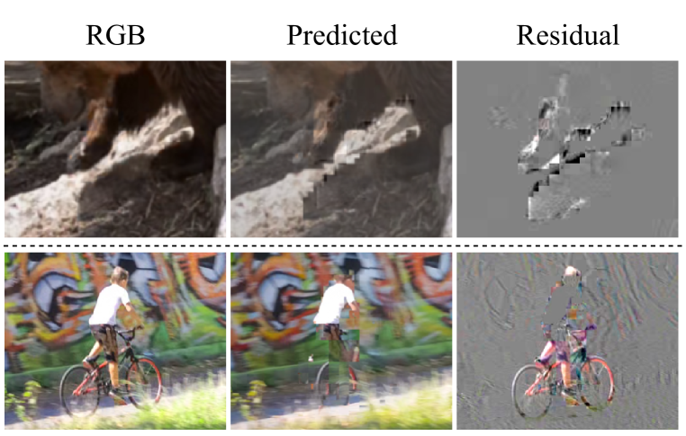
Figure 2: Bar plots of a GOP visualizing frame assignments and the relative frame size. The ‘bmx-trees’ sequence has faster movements so it has more I-/P-frames than ‘bear’ (37.5% vs. 23.2%). The red arrows mark displayed frames, which feature examples of block effects for the ‘bear’ sequence above and motion vector estimation failures for the ‘bmx-trees’ sequence below.

3.2 Motion compensation in compressed videos

A key difference between optical flow and motion vectors is that optical flow is a dense vector field with respect to a neighbouring frame in time, whereas motion vectors are block-wise displacements with respect to arbitrary reference frame(s) within the GOP. The associated blocks are called Prediction Units (PU), and they vary in size from $64\!\times\!64$ to $8\!\times\!4$ or $\!4\times\!8$ pixels. PUs can be uni-directional, with reference frames from either the past or the future, or bi-directional, with references to both the past and the future. P-frames have only uni-directional PUs, while B-frames have both uni-directional and bi-directional PUs.

In this work, we denote a PU as $\Omega_{ij}$, with constituent pixels $(x,y)\in\Omega_{ij}$, where $i$ indexes the frame and $j$ indexes the PU in frame $i$. In the general bi-directional case, $\Omega_{ij}$ is associated with a pair of forward and backward motion vectors $(\vec{\mathbf{v}}_{ij},{\mathchoice{\vbox{\offinterlineskip\halign{#\cr\reflectbox{$\displaystyle\vec{}\mkern 4.0mu$}\cr\kern-4.30554pt\cr$\displaystyle\mathbf{v}$\cr}}}{\vbox{\offinterlineskip\halign{#\cr\reflectbox{$\textstyle\vec{}\mkern 4.0mu$}\cr\kern-4.30554pt\cr$\textstyle\mathbf{v}$\cr}}}{\vbox{\offinterlineskip\halign{#\cr\reflectbox{$\scriptstyle\vec{}\mkern 4.0mu$}\cr\kern-3.01389pt\cr$\scriptstyle\mathbf{v}$\cr}}}{\vbox{\offinterlineskip\halign{#\cr\reflectbox{$\scriptscriptstyle\vec{}\mkern 4.0mu$}\cr\kern-2.15277pt\cr$\scriptscriptstyle\mathbf{v}$\cr}}}}_{ij})$, where the right and left arrows denote forward and backward motion, respectively. The forward motion vector $\vec{\mathbf{v}}_{ij}=[\vec{u},\vec{v},\vec{t}\,]$ is given by displacements $\vec{u}$ and $\vec{v}$ and reference frame $\vec{t}$, where $\vec{t}\!<\!i$; analogously, ${\mathchoice{\vbox{\offinterlineskip\halign{#\cr\reflectbox{$\displaystyle\vec{}\mkern 4.0mu$}\cr\kern-4.30554pt\cr$\displaystyle\mathbf{v}$\cr}}}{\vbox{\offinterlineskip\halign{#\cr\reflectbox{$\textstyle\vec{}\mkern 4.0mu$}\cr\kern-4.30554pt\cr$\textstyle\mathbf{v}$\cr}}}{\vbox{\offinterlineskip\halign{#\cr\reflectbox{$\scriptstyle\vec{}\mkern 4.0mu$}\cr\kern-3.01389pt\cr$\scriptstyle\mathbf{v}$\cr}}}{\vbox{\offinterlineskip\halign{#\cr\reflectbox{$\scriptscriptstyle\vec{}\mkern 4.0mu$}\cr\kern-2.15277pt\cr$\scriptscriptstyle\mathbf{v}$\cr}}}}_{ij}=[{\mathchoice{\vbox{\offinterlineskip\halign{#\cr\reflectbox{$\displaystyle\vec{}\mkern 4.0mu$}\cr\kern-4.30554pt\cr$\displaystyle u$\cr}}}{\vbox{\offinterlineskip\halign{#\cr\reflectbox{$\textstyle\vec{}\mkern 4.0mu$}\cr\kern-4.30554pt\cr$\textstyle u$\cr}}}{\vbox{\offinterlineskip\halign{#\cr\reflectbox{$\scriptstyle\vec{}\mkern 4.0mu$}\cr\kern-3.01389pt\cr$\scriptstyle u$\cr}}}{\vbox{\offinterlineskip\halign{#\cr\reflectbox{$\scriptscriptstyle\vec{}\mkern 4.0mu$}\cr\kern-2.15277pt\cr$\scriptscriptstyle u$\cr}}}},{\mathchoice{\vbox{\offinterlineskip\halign{#\cr\reflectbox{$\displaystyle\vec{}\mkern 4.0mu$}\cr\kern-4.30554pt\cr$\displaystyle v$\cr}}}{\vbox{\offinterlineskip\halign{#\cr\reflectbox{$\textstyle\vec{}\mkern 4.0mu$}\cr\kern-4.30554pt\cr$\textstyle v$\cr}}}{\vbox{\offinterlineskip\halign{#\cr\reflectbox{$\scriptstyle\vec{}\mkern 4.0mu$}\cr\kern-3.01389pt\cr$\scriptstyle v$\cr}}}{\vbox{\offinterlineskip\halign{#\cr\reflectbox{$\scriptscriptstyle\vec{}\mkern 4.0mu$}\cr\kern-2.15277pt\cr$\scriptscriptstyle v$\cr}}}},{\mathchoice{\vbox{\offinterlineskip\halign{#\cr\reflectbox{$\displaystyle\vec{}\mkern 4.0mu$}\cr\kern-4.30554pt\cr$\displaystyle t$\cr}}}{\vbox{\offinterlineskip\halign{#\cr\reflectbox{$\textstyle\vec{}\mkern 4.0mu$}\cr\kern-4.30554pt\cr$\textstyle t$\cr}}}{\vbox{\offinterlineskip\halign{#\cr\reflectbox{$\scriptstyle\vec{}\mkern 4.0mu$}\cr\kern-3.01389pt\cr$\scriptstyle t$\cr}}}{\vbox{\offinterlineskip\halign{#\cr\reflectbox{$\scriptscriptstyle\vec{}\mkern 4.0mu$}\cr\kern-2.15277pt\cr$\scriptscriptstyle t$\cr}}}}\,]$ denotes a backward motion vector with displacements $[{\mathchoice{\vbox{\offinterlineskip\halign{#\cr\reflectbox{$\displaystyle\vec{}\mkern 4.0mu$}\cr\kern-4.30554pt\cr$\displaystyle u$\cr}}}{\vbox{\offinterlineskip\halign{#\cr\reflectbox{$\textstyle\vec{}\mkern 4.0mu$}\cr\kern-4.30554pt\cr$\textstyle u$\cr}}}{\vbox{\offinterlineskip\halign{#\cr\reflectbox{$\scriptstyle\vec{}\mkern 4.0mu$}\cr\kern-3.01389pt\cr$\scriptstyle u$\cr}}}{\vbox{\offinterlineskip\halign{#\cr\reflectbox{$\scriptscriptstyle\vec{}\mkern 4.0mu$}\cr\kern-2.15277pt\cr$\scriptscriptstyle u$\cr}}}},{\mathchoice{\vbox{\offinterlineskip\halign{#\cr\reflectbox{$\displaystyle\vec{}\mkern 4.0mu$}\cr\kern-4.30554pt\cr$\displaystyle v$\cr}}}{\vbox{\offinterlineskip\halign{#\cr\reflectbox{$\textstyle\vec{}\mkern 4.0mu$}\cr\kern-4.30554pt\cr$\textstyle v$\cr}}}{\vbox{\offinterlineskip\halign{#\cr\reflectbox{$\scriptstyle\vec{}\mkern 4.0mu$}\cr\kern-3.01389pt\cr$\scriptstyle v$\cr}}}{\vbox{\offinterlineskip\halign{#\cr\reflectbox{$\scriptscriptstyle\vec{}\mkern 4.0mu$}\cr\kern-2.15277pt\cr$\scriptscriptstyle v$\cr}}}}]$ and reference frame $\textstyle\vec{}\mkern 4.0mu$ $\textstyle t$ , where ${\mathchoice{\vbox{\offinterlineskip\halign{#\cr\reflectbox{$\displaystyle\vec{}\mkern 4.0mu$}\cr\kern-4.30554pt\cr$\displaystyle t$\cr}}}{\vbox{\offinterlineskip\halign{#\cr\reflectbox{$\textstyle\vec{}\mkern 4.0mu$}\cr\kern-4.30554pt\cr$\textstyle t$\cr}}}{\vbox{\offinterlineskip\halign{#\cr\reflectbox{$\scriptstyle\vec{}\mkern 4.0mu$}\cr\kern-3.01389pt\cr$\scriptstyle t$\cr}}}{\vbox{\offinterlineskip\halign{#\cr\reflectbox{$\scriptscriptstyle\vec{}\mkern 4.0mu$}\cr\kern-2.15277pt\cr$\scriptscriptstyle t$\cr}}}}\!>\!i$.

Based on the motion vectors, the pixels $(x,y)\!\in\!\Omega_{ij}$ can be predicted from co-located blocks of the same size as $\Omega_{ij}$ from reference frames $I_{\vec{t}}$ and $I_{{\mathchoice{\vbox{\offinterlineskip\halign{#\cr\reflectbox{$\displaystyle\vec{}\mkern 4.0mu$}\cr\kern-3.01389pt\cr$\displaystyle t$\cr}}}{\vbox{\offinterlineskip\halign{#\cr\reflectbox{$\textstyle\vec{}\mkern 4.0mu$}\cr\kern-3.01389pt\cr$\textstyle t$\cr}}}{\vbox{\offinterlineskip\halign{#\cr\reflectbox{$\scriptstyle\vec{}\mkern 4.0mu$}\cr\kern-2.10971pt\cr$\scriptstyle t$\cr}}}{\vbox{\offinterlineskip\halign{#\cr\reflectbox{$\scriptscriptstyle\vec{}\mkern 4.0mu$}\cr\kern-1.50694pt\cr$\scriptscriptstyle t$\cr}}}}}$. The reconstructed frame $\hat{I}_{i}^{x,y}$ at $(x,y)$ of frame $i$, for $(x,y)\in\Omega_{ij}$, is given as

$$\hat{I}_{i}^{x,y}=\vec{w}I_{\vec{t}\,}^{x+\vec{u},y+\vec{v}}+{\mathchoice{\vbox{\offinterlineskip\halign{#\cr\reflectbox{$\displaystyle\vec{}\mkern 4.0mu$}\cr\kern-4.30554pt\cr$\displaystyle w$\cr}}}{\vbox{\offinterlineskip\halign{#\cr\reflectbox{$\textstyle\vec{}\mkern 4.0mu$}\cr\kern-4.30554pt\cr$\textstyle w$\cr}}}{\vbox{\offinterlineskip\halign{#\cr\reflectbox{$\scriptstyle\vec{}\mkern 4.0mu$}\cr\kern-3.01389pt\cr$\scriptstyle w$\cr}}}{\vbox{\offinterlineskip\halign{#\cr\reflectbox{$\scriptscriptstyle\vec{}\mkern 4.0mu$}\cr\kern-2.15277pt\cr$\scriptscriptstyle w$\cr}}}}I_{{\mathchoice{\vbox{\offinterlineskip\halign{#\cr\reflectbox{$\displaystyle\vec{}\mkern 4.0mu$}\cr\kern-3.01389pt\cr$\displaystyle t$\cr}}}{\vbox{\offinterlineskip\halign{#\cr\reflectbox{$\textstyle\vec{}\mkern 4.0mu$}\cr\kern-3.01389pt\cr$\textstyle t$\cr}}}{\vbox{\offinterlineskip\halign{#\cr\reflectbox{$\scriptstyle\vec{}\mkern 4.0mu$}\cr\kern-2.10971pt\cr$\scriptstyle t$\cr}}}{\vbox{\offinterlineskip\halign{#\cr\reflectbox{$\scriptscriptstyle\vec{}\mkern 4.0mu$}\cr\kern-1.50694pt\cr$\scriptscriptstyle t$\cr}}}}}^{x+{\mathchoice{\vbox{\offinterlineskip\halign{#\cr\reflectbox{$\displaystyle\vec{}\mkern 4.0mu$}\cr\kern-3.01389pt\cr$\displaystyle u$\cr}}}{\vbox{\offinterlineskip\halign{#\cr\reflectbox{$\textstyle\vec{}\mkern 4.0mu$}\cr\kern-3.01389pt\cr$\textstyle u$\cr}}}{\vbox{\offinterlineskip\halign{#\cr\reflectbox{$\scriptstyle\vec{}\mkern 4.0mu$}\cr\kern-2.10971pt\cr$\scriptstyle u$\cr}}}{\vbox{\offinterlineskip\halign{#\cr\reflectbox{$\scriptscriptstyle\vec{}\mkern 4.0mu$}\cr\kern-1.50694pt\cr$\scriptscriptstyle u$\cr}}}},y+{\mathchoice{\vbox{\offinterlineskip\halign{#\cr\reflectbox{$\displaystyle\vec{}\mkern 4.0mu$}\cr\kern-3.01389pt\cr$\displaystyle v$\cr}}}{\vbox{\offinterlineskip\halign{#\cr\reflectbox{$\textstyle\vec{}\mkern 4.0mu$}\cr\kern-3.01389pt\cr$\textstyle v$\cr}}}{\vbox{\offinterlineskip\halign{#\cr\reflectbox{$\scriptstyle\vec{}\mkern 4.0mu$}\cr\kern-2.10971pt\cr$\scriptstyle v$\cr}}}{\vbox{\offinterlineskip\halign{#\cr\reflectbox{$\scriptscriptstyle\vec{}\mkern 4.0mu$}\cr\kern-1.50694pt\cr$\scriptscriptstyle v$\cr}}}}},$$ (1)

where $(\vec{w},{\mathchoice{\vbox{\offinterlineskip\halign{#\cr\reflectbox{$\displaystyle\vec{}\mkern 4.0mu$}\cr\kern-4.30554pt\cr$\displaystyle w$\cr}}}{\vbox{\offinterlineskip\halign{#\cr\reflectbox{$\textstyle\vec{}\mkern 4.0mu$}\cr\kern-4.30554pt\cr$\textstyle w$\cr}}}{\vbox{\offinterlineskip\halign{#\cr\reflectbox{$\scriptstyle\vec{}\mkern 4.0mu$}\cr\kern-3.01389pt\cr$\scriptstyle w$\cr}}}{\vbox{\offinterlineskip\halign{#\cr\reflectbox{$\scriptscriptstyle\vec{}\mkern 4.0mu$}\cr\kern-2.15277pt\cr$\scriptscriptstyle w$\cr}}}})$ are weighting components for the forward and backward motions, respectively, and $\vec{w}\!+\!{\mathchoice{\vbox{\offinterlineskip\halign{#\cr\reflectbox{$\displaystyle\vec{}\mkern 4.0mu$}\cr\kern-4.30554pt\cr$\displaystyle w$\cr}}}{\vbox{\offinterlineskip\halign{#\cr\reflectbox{$\textstyle\vec{}\mkern 4.0mu$}\cr\kern-4.30554pt\cr$\textstyle w$\cr}}}{\vbox{\offinterlineskip\halign{#\cr\reflectbox{$\scriptstyle\vec{}\mkern 4.0mu$}\cr\kern-3.01389pt\cr$\scriptstyle w$\cr}}}{\vbox{\offinterlineskip\halign{#\cr\reflectbox{$\scriptscriptstyle\vec{}\mkern 4.0mu$}\cr\kern-2.15277pt\cr$\scriptscriptstyle w$\cr}}}}\!=\!1$. In the case of a uni-directional PU, either $\vec{w}$ or $\textstyle\vec{}\mkern 4.0mu$ $\textstyle w$ would be set to $0$ and the corresponding $\vec{\mathbf{v}}$ or $\textstyle\vec{}\mkern 4.0mu$ $\textstyle\mathbf{v}$ is undefined.

In older and more restrictive codec settings, such as those used in CVOS[32], reference frames were limited to I-frames. Modern codecs like HEVC, i.e. what we consider in this work, allow P- and B-frames to reference pixels in other P- and B-frames, which are themselves reconstructed from other references. This makes the reconstruction in Eq. 1 multi-hop, which improves overall coding efficiency as the drifting problem can be alleviated with smaller temporal reference distance. Examples of PUs and frame predictions are illustrated in Fig. 3. Motion vectors are inherently coarse and noisy, due to their block-wise nature and encoding errors in areas of fast and abrupt movements (see examples in Fig. 2). As such, the remaining differences between the RGB image $I_{i}$ and prediction $\hat{I}_{i}$ at frame $i$ are stored in the residual $\textbf{e}_{i}$ to recover pixel-level detailing:

$$I_{i}=\hat{I}_{i}+\textbf{e}_{i}.$$ (2)

In principle, $\textbf{e}_{i}$ is sparse; the sparsity is directly correlated with the accuracy of the motion vector prediction. The key to efficient video encoding is balancing the storage savings of using larger PUs for P- and B-frames, i.e. fewer motion vectors, versus requiring less sparse residuals to compensate for the coarser block motions.

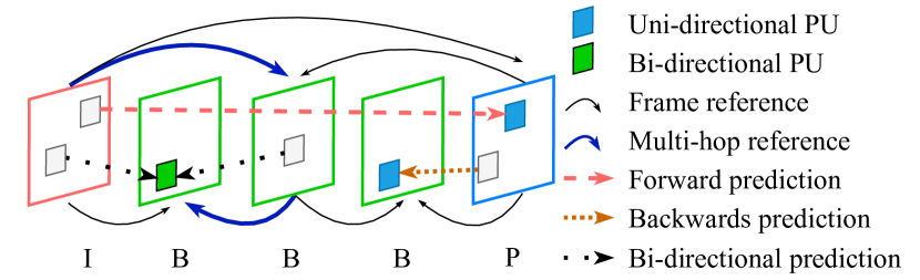
Figure 3: GOP schematic. Dashed lines denote motion compensation in prediction blocks. ’I’, ’B’ and ’P’ denote frame types.

3.3 Dense frame-wise motion representation

Performing frame-wise propagation directly from the motion vectors can be cumbersome as the vectors are defined block-wise according to PUs. The PUs in a given frame often have several (different) references over multiple hops. As such, we compute a dense frame-wise motion field to serve as a more convenient intermediate representation. Specifically, we define a bi-directional motion field as $M_{i}\!=\![\vec{M}_{i},{\mathchoice{\vbox{\offinterlineskip\halign{#\cr\reflectbox{$\displaystyle\vec{}\mkern 4.0mu$}\cr\kern-4.30554pt\cr$\displaystyle M$\cr}}}{\vbox{\offinterlineskip\halign{#\cr\reflectbox{$\textstyle\vec{}\mkern 4.0mu$}\cr\kern-4.30554pt\cr$\textstyle M$\cr}}}{\vbox{\offinterlineskip\halign{#\cr\reflectbox{$\scriptstyle\vec{}\mkern 4.0mu$}\cr\kern-3.01389pt\cr$\scriptstyle M$\cr}}}{\vbox{\offinterlineskip\halign{#\cr\reflectbox{$\scriptscriptstyle\vec{}\mkern 4.0mu$}\cr\kern-2.15277pt\cr$\scriptscriptstyle M$\cr}}}}_{i}]$, where $\vec{M}_{i}\!\in\!\mathbb{R}^{H\times W\times 3}$ is a dense pixel-wise representation of forward motions for frame $i$ and is represented by $[\vec{u},\vec{v},\vec{t}\,]$, i.e. the displacements and the reference frame. Similar to the motion vectors, the right- and left-arrowed accents denote forward and backward motions respectively. As such, ${\mathchoice{\vbox{\offinterlineskip\halign{#\cr\reflectbox{$\displaystyle\vec{}\mkern 4.0mu$}\cr\kern-4.30554pt\cr$\displaystyle M$\cr}}}{\vbox{\offinterlineskip\halign{#\cr\reflectbox{$\textstyle\vec{}\mkern 4.0mu$}\cr\kern-4.30554pt\cr$\textstyle M$\cr}}}{\vbox{\offinterlineskip\halign{#\cr\reflectbox{$\scriptstyle\vec{}\mkern 4.0mu$}\cr\kern-3.01389pt\cr$\scriptstyle M$\cr}}}{\vbox{\offinterlineskip\halign{#\cr\reflectbox{$\scriptscriptstyle\vec{}\mkern 4.0mu$}\cr\kern-2.15277pt\cr$\scriptscriptstyle M$\cr}}}}_{i}\!\in\!\mathbb{R}^{H\times W\times 3}$ stores backward motions for frame $i$ represented by $[{\mathchoice{\vbox{\offinterlineskip\halign{#\cr\reflectbox{$\displaystyle\vec{}\mkern 4.0mu$}\cr\kern-4.30554pt\cr$\displaystyle u$\cr}}}{\vbox{\offinterlineskip\halign{#\cr\reflectbox{$\textstyle\vec{}\mkern 4.0mu$}\cr\kern-4.30554pt\cr$\textstyle u$\cr}}}{\vbox{\offinterlineskip\halign{#\cr\reflectbox{$\scriptstyle\vec{}\mkern 4.0mu$}\cr\kern-3.01389pt\cr$\scriptstyle u$\cr}}}{\vbox{\offinterlineskip\halign{#\cr\reflectbox{$\scriptscriptstyle\vec{}\mkern 4.0mu$}\cr\kern-2.15277pt\cr$\scriptscriptstyle u$\cr}}}},{\mathchoice{\vbox{\offinterlineskip\halign{#\cr\reflectbox{$\displaystyle\vec{}\mkern 4.0mu$}\cr\kern-4.30554pt\cr$\displaystyle v$\cr}}}{\vbox{\offinterlineskip\halign{#\cr\reflectbox{$\textstyle\vec{}\mkern 4.0mu$}\cr\kern-4.30554pt\cr$\textstyle v$\cr}}}{\vbox{\offinterlineskip\halign{#\cr\reflectbox{$\scriptstyle\vec{}\mkern 4.0mu$}\cr\kern-3.01389pt\cr$\scriptstyle v$\cr}}}{\vbox{\offinterlineskip\halign{#\cr\reflectbox{$\scriptscriptstyle\vec{}\mkern 4.0mu$}\cr\kern-2.15277pt\cr$\scriptscriptstyle v$\cr}}}},{\mathchoice{\vbox{\offinterlineskip\halign{#\cr\reflectbox{$\displaystyle\vec{}\mkern 4.0mu$}\cr\kern-4.30554pt\cr$\displaystyle t$\cr}}}{\vbox{\offinterlineskip\halign{#\cr\reflectbox{$\textstyle\vec{}\mkern 4.0mu$}\cr\kern-4.30554pt\cr$\textstyle t$\cr}}}{\vbox{\offinterlineskip\halign{#\cr\reflectbox{$\scriptstyle\vec{}\mkern 4.0mu$}\cr\kern-3.01389pt\cr$\scriptstyle t$\cr}}}{\vbox{\offinterlineskip\halign{#\cr\reflectbox{$\scriptscriptstyle\vec{}\mkern 4.0mu$}\cr\kern-2.15277pt\cr$\scriptscriptstyle t$\cr}}}}\,]$. The motion components are determined by aggregating all the PUs $\{\Omega_{ij}\},j\in\{1...J_{i}\}$, where $J_{i}$ is the total number of PUs in frame $i$. i.e.

$$\vec{\mathbf{v}}_{\Omega,i}\rightarrow\vec{M}_{i}^{x,y};\quad{\mathchoice{\vbox{\offinterlineskip\halign{#\cr\reflectbox{$\displaystyle\vec{}\mkern 4.0mu$}\cr\kern-4.30554pt\cr$\displaystyle\mathbf{v}$\cr}}}{\vbox{\offinterlineskip\halign{#\cr\reflectbox{$\textstyle\vec{}\mkern 4.0mu$}\cr\kern-4.30554pt\cr$\textstyle\mathbf{v}$\cr}}}{\vbox{\offinterlineskip\halign{#\cr\reflectbox{$\scriptstyle\vec{}\mkern 4.0mu$}\cr\kern-3.01389pt\cr$\scriptstyle\mathbf{v}$\cr}}}{\vbox{\offinterlineskip\halign{#\cr\reflectbox{$\scriptscriptstyle\vec{}\mkern 4.0mu$}\cr\kern-2.15277pt\cr$\scriptscriptstyle\mathbf{v}$\cr}}}}_{\Omega,i}\rightarrow{\mathchoice{\vbox{\offinterlineskip\halign{#\cr\reflectbox{$\displaystyle\vec{}\mkern 4.0mu$}\cr\kern-4.30554pt\cr$\displaystyle M$\cr}}}{\vbox{\offinterlineskip\halign{#\cr\reflectbox{$\textstyle\vec{}\mkern 4.0mu$}\cr\kern-4.30554pt\cr$\textstyle M$\cr}}}{\vbox{\offinterlineskip\halign{#\cr\reflectbox{$\scriptstyle\vec{}\mkern 4.0mu$}\cr\kern-3.01389pt\cr$\scriptstyle M$\cr}}}{\vbox{\offinterlineskip\halign{#\cr\reflectbox{$\scriptscriptstyle\vec{}\mkern 4.0mu$}\cr\kern-2.15277pt\cr$\scriptscriptstyle M$\cr}}}}_{i}^{x,y},\quad(x,y)\in\Omega_{ij}.$$ (3)

This assignment procedure, which is denoted by $\rightarrow$, iterates through all the spatial locations of frame $i$. If a given PU in the B-frame is uni-directional, then the elements in the opposite direction in either $\vec{M}$ or $\textstyle\vec{}\mkern 4.0mu$ $\textstyle M$ is set to zero accordingly. For pixels where $\textstyle\vec{}\mkern 4.0mu$ $\textstyle t$ or $\vec{t}$ is directed to a keyframe, the prediction is single-hop; for pixels where $\textstyle\vec{}\mkern 4.0mu$ $\textstyle t$ or $\vec{t}$ is directed to another non-keyframe, this will be multi-hop as the current reference is chained to further references.

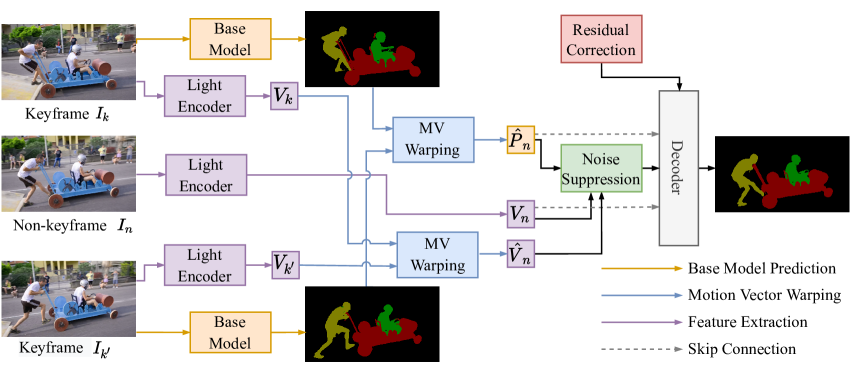
Figure 4: Overall framework. Keyframe segmentation predictions are propagated to non-keyframes through a soft motion vector propagation module that suppresses inaccurate motion vectors. Propagated masks are then corrected based on the residuals and feature matching.

4 Methodology

We accelerate off-the-shelf VOS methods by applying these methods as a base network to selected keyframes (Sec. 4.4). The keyframe segmentations are propagated to non-keyframes with a soft motion vector propagation module (Sec. 4.2) and further refined via a residual-based correction module (Sec. 4.3).  Fig. 4 illustrates the overall framework. The acceleration comes from the computational savings of propagation and correction compared to applying the base network to all frames in the sequence.

4.1 Problem formulation

We denote the decoded sequence from a compressed video bitstream of length $T$ as $\{(I_{i},M_{i},\textbf{e}_{i}),i\in[1,T]\}$.

For convenience, we directly use the motion field $M_{i}$ instead of the raw motion vectors. Note that after decoding, we already have access to the RGB image $I_{i}$ for frame $i$. For $P$ and $B$ frames, $I_{i}$ is reconstructed from the motion-predicted frame $\hat{I}_{i}$ and the residual $\textbf{e}_{i}$ based on Eq. 2. For clarity, we maintain two redundant frame indices $n$ and $k$ for referring to non-keyframes and keyframes, respectively. We denote the base network as $\{F,G\}$. The first portion of the network $F$ extracts low-level appearance features $V_{k}$ from the input keyframe $I_{k}$; $G$ denotes the subsequent part of the network that further processes $V_{k}$ to estimate the segmentation $P_{k}$, i.e., for a keyframe $k$,

$$V_{k}=F(I_{k}),\;\;P_{k}=G(V_{k}),$$ (4)

where $P_{k}\in\mathbb{R}^{H\times W\times O}$ and $V_{k}\in\mathbb{R}^{H\times W\times C}$. Here, $O$ is the number of objects in the video sequence, $C$ is the number of channels for the low-level feature and $H\times W$ is the spatial resolution of the prediction.

For a non-keyframe $I_{n}$, a standard approach [45] to propagate the segmentation predictions from a keyframe $k$ is to apply a warp based on the optical flow:

$$\tilde{P}_{n}=W(\text{OF}_{n},P_{k}),$$ (5)

where $W$ is the warping operation, $OF_{n}$ is the optical flow between $P_{n}$ and $P_{k}$, and $\tilde{P}$ is the propagated predictions. This form of propagation has two key drawbacks. Firstly, most schemes use optical flow computed only between two frames, which increases the possible errors that arise from occlusion. Secondly, estimating accurate optical flows still comes with considerable computational expense.

4.2 Soft motion-vector propagation module

In this section, we outline how motion vectors, specifically the motion vector field $M_{n}$ defined in Eq. 3 for a non-keyframe $I_{n}$, can be used in place of optical flow $\text{OF}_{n}$ in Eq. 5. We first introduce the motion vector warping operation, in which $\hat{P}_{n}$ and $\hat{V}_{n}$ denote the motion vector warped prediction and warped features, i.e.

$$\hat{P}_{n}=W_{MV}(M_{n},P_{\star}),\quad\hat{V}_{n}=W_{MV}(M_{n},V_{\star}),$$ (6)

where $P_{\star}$ and $V_{\star}$ denote the corresponding segmentations and features for key- and non-key reference frames, respectively. The warping operation $W_{MV}$ is defined as a backward warp which iterates over all the spatial locations of frame $n$. If we denote with $\Lambda$ the item, i.e. $P_{\star}$ or $V_{\star}$, to be propagated, such that $\hat{\Lambda}_{n}=W_{MV}(M_{n},\Lambda)$, then the propagated value at $(x,y)$ for a non-keyframe $n$, based on Eq. 1 can be defined as:

$$\hat{\Lambda}_{n}^{x,y}=\begin{cases}\Lambda_{{\mathchoice{\vbox{\offinterlineskip\halign{#\cr\reflectbox{$\displaystyle\vec{}\mkern 4.0mu$}\cr\kern-3.01389pt\cr$\displaystyle t$\cr}}}{\vbox{\offinterlineskip\halign{#\cr\reflectbox{$\textstyle\vec{}\mkern 4.0mu$}\cr\kern-3.01389pt\cr$\textstyle t$\cr}}}{\vbox{\offinterlineskip\halign{#\cr\reflectbox{$\scriptstyle\vec{}\mkern 4.0mu$}\cr\kern-2.10971pt\cr$\scriptstyle t$\cr}}}{\vbox{\offinterlineskip\halign{#\cr\reflectbox{$\scriptscriptstyle\vec{}\mkern 4.0mu$}\cr\kern-1.50694pt\cr$\scriptscriptstyle t$\cr}}}}}^{x+{\mathchoice{\vbox{\offinterlineskip\halign{#\cr\reflectbox{$\displaystyle\vec{}\mkern 4.0mu$}\cr\kern-3.01389pt\cr$\displaystyle u$\cr}}}{\vbox{\offinterlineskip\halign{#\cr\reflectbox{$\textstyle\vec{}\mkern 4.0mu$}\cr\kern-3.01389pt\cr$\textstyle u$\cr}}}{\vbox{\offinterlineskip\halign{#\cr\reflectbox{$\scriptstyle\vec{}\mkern 4.0mu$}\cr\kern-2.10971pt\cr$\scriptstyle u$\cr}}}{\vbox{\offinterlineskip\halign{#\cr\reflectbox{$\scriptscriptstyle\vec{}\mkern 4.0mu$}\cr\kern-1.50694pt\cr$\scriptscriptstyle u$\cr}}}},y+{\mathchoice{\vbox{\offinterlineskip\halign{#\cr\reflectbox{$\displaystyle\vec{}\mkern 4.0mu$}\cr\kern-3.01389pt\cr$\displaystyle v$\cr}}}{\vbox{\offinterlineskip\halign{#\cr\reflectbox{$\textstyle\vec{}\mkern 4.0mu$}\cr\kern-3.01389pt\cr$\textstyle v$\cr}}}{\vbox{\offinterlineskip\halign{#\cr\reflectbox{$\scriptstyle\vec{}\mkern 4.0mu$}\cr\kern-2.10971pt\cr$\scriptstyle v$\cr}}}{\vbox{\offinterlineskip\halign{#\cr\reflectbox{$\scriptscriptstyle\vec{}\mkern 4.0mu$}\cr\kern-1.50694pt\cr$\scriptscriptstyle v$\cr}}}}},\quad&\text{if}\;\vec{t}=0,\\ \Lambda_{\vec{t}}^{x+\vec{u},y+\vec{v}},\quad&\text{if}\;{\mathchoice{\vbox{\offinterlineskip\halign{#\cr\reflectbox{$\displaystyle\vec{}\mkern 4.0mu$}\cr\kern-4.30554pt\cr$\displaystyle t$\cr}}}{\vbox{\offinterlineskip\halign{#\cr\reflectbox{$\textstyle\vec{}\mkern 4.0mu$}\cr\kern-4.30554pt\cr$\textstyle t$\cr}}}{\vbox{\offinterlineskip\halign{#\cr\reflectbox{$\scriptstyle\vec{}\mkern 4.0mu$}\cr\kern-3.01389pt\cr$\scriptstyle t$\cr}}}{\vbox{\offinterlineskip\halign{#\cr\reflectbox{$\scriptscriptstyle\vec{}\mkern 4.0mu$}\cr\kern-2.15277pt\cr$\scriptscriptstyle t$\cr}}}}=0,\\ \frac{1}{2}\Lambda_{{\mathchoice{\vbox{\offinterlineskip\halign{#\cr\reflectbox{$\displaystyle\vec{}\mkern 4.0mu$}\cr\kern-3.01389pt\cr$\displaystyle t$\cr}}}{\vbox{\offinterlineskip\halign{#\cr\reflectbox{$\textstyle\vec{}\mkern 4.0mu$}\cr\kern-3.01389pt\cr$\textstyle t$\cr}}}{\vbox{\offinterlineskip\halign{#\cr\reflectbox{$\scriptstyle\vec{}\mkern 4.0mu$}\cr\kern-2.10971pt\cr$\scriptstyle t$\cr}}}{\vbox{\offinterlineskip\halign{#\cr\reflectbox{$\scriptscriptstyle\vec{}\mkern 4.0mu$}\cr\kern-1.50694pt\cr$\scriptscriptstyle t$\cr}}}}}^{x+{\mathchoice{\vbox{\offinterlineskip\halign{#\cr\reflectbox{$\displaystyle\vec{}\mkern 4.0mu$}\cr\kern-3.01389pt\cr$\displaystyle u$\cr}}}{\vbox{\offinterlineskip\halign{#\cr\reflectbox{$\textstyle\vec{}\mkern 4.0mu$}\cr\kern-3.01389pt\cr$\textstyle u$\cr}}}{\vbox{\offinterlineskip\halign{#\cr\reflectbox{$\scriptstyle\vec{}\mkern 4.0mu$}\cr\kern-2.10971pt\cr$\scriptstyle u$\cr}}}{\vbox{\offinterlineskip\halign{#\cr\reflectbox{$\scriptscriptstyle\vec{}\mkern 4.0mu$}\cr\kern-1.50694pt\cr$\scriptscriptstyle u$\cr}}}},y+{\mathchoice{\vbox{\offinterlineskip\halign{#\cr\reflectbox{$\displaystyle\vec{}\mkern 4.0mu$}\cr\kern-3.01389pt\cr$\displaystyle v$\cr}}}{\vbox{\offinterlineskip\halign{#\cr\reflectbox{$\textstyle\vec{}\mkern 4.0mu$}\cr\kern-3.01389pt\cr$\textstyle v$\cr}}}{\vbox{\offinterlineskip\halign{#\cr\reflectbox{$\scriptstyle\vec{}\mkern 4.0mu$}\cr\kern-2.10971pt\cr$\scriptstyle v$\cr}}}{\vbox{\offinterlineskip\halign{#\cr\reflectbox{$\scriptscriptstyle\vec{}\mkern 4.0mu$}\cr\kern-1.50694pt\cr$\scriptscriptstyle v$\cr}}}}}+\frac{1}{2}\Lambda_{\vec{t}}^{x+\vec{u},y+\vec{v}},\quad&\text{otherwise}.\end{cases}$$ (7)

$$\text{where:}\qquad\qquad[\vec{u},\vec{v},\vec{t},{\mathchoice{\vbox{\offinterlineskip\halign{#\cr\reflectbox{$\displaystyle\vec{}\mkern 4.0mu$}\cr\kern-4.30554pt\cr$\displaystyle u$\cr}}}{\vbox{\offinterlineskip\halign{#\cr\reflectbox{$\textstyle\vec{}\mkern 4.0mu$}\cr\kern-4.30554pt\cr$\textstyle u$\cr}}}{\vbox{\offinterlineskip\halign{#\cr\reflectbox{$\scriptstyle\vec{}\mkern 4.0mu$}\cr\kern-3.01389pt\cr$\scriptstyle u$\cr}}}{\vbox{\offinterlineskip\halign{#\cr\reflectbox{$\scriptscriptstyle\vec{}\mkern 4.0mu$}\cr\kern-2.15277pt\cr$\scriptscriptstyle u$\cr}}}},{\mathchoice{\vbox{\offinterlineskip\halign{#\cr\reflectbox{$\displaystyle\vec{}\mkern 4.0mu$}\cr\kern-4.30554pt\cr$\displaystyle v$\cr}}}{\vbox{\offinterlineskip\halign{#\cr\reflectbox{$\textstyle\vec{}\mkern 4.0mu$}\cr\kern-4.30554pt\cr$\textstyle v$\cr}}}{\vbox{\offinterlineskip\halign{#\cr\reflectbox{$\scriptstyle\vec{}\mkern 4.0mu$}\cr\kern-3.01389pt\cr$\scriptstyle v$\cr}}}{\vbox{\offinterlineskip\halign{#\cr\reflectbox{$\scriptscriptstyle\vec{}\mkern 4.0mu$}\cr\kern-2.15277pt\cr$\scriptscriptstyle v$\cr}}}},{\mathchoice{\vbox{\offinterlineskip\halign{#\cr\reflectbox{$\displaystyle\vec{}\mkern 4.0mu$}\cr\kern-4.30554pt\cr$\displaystyle t$\cr}}}{\vbox{\offinterlineskip\halign{#\cr\reflectbox{$\textstyle\vec{}\mkern 4.0mu$}\cr\kern-4.30554pt\cr$\textstyle t$\cr}}}{\vbox{\offinterlineskip\halign{#\cr\reflectbox{$\scriptstyle\vec{}\mkern 4.0mu$}\cr\kern-3.01389pt\cr$\scriptstyle t$\cr}}}{\vbox{\offinterlineskip\halign{#\cr\reflectbox{$\scriptscriptstyle\vec{}\mkern 4.0mu$}\cr\kern-2.15277pt\cr$\scriptscriptstyle t$\cr}}}}\;]=M_{n}^{x,y}.$$ (8)

The first two cases in  Eq. 7 are for warping unidirectional motion vectors forwards and backwards in time, respectively, and the third case is used for bi-directional motion vectors. Note that in the third case, the forward and backward motion vectors are equally weighted and not according to $\vec{w}$ and $\textstyle\vec{}\mkern 4.0mu$ $\textstyle w$ from Eq. 1. This is because we interpret the references to be equally indicative of the target mask; also, $\vec{w}$ and $\textstyle\vec{}\mkern 4.0mu$ $\textstyle w$ are tuned for reconstructing the target RGB pixel value. In the case when $u$, $v$ are not integers, nearest-neighbours or bilinear interpolation will be applied in the reference map; for simplicity, we omit the interpolation in the formulation. If the reference frame $\textstyle\vec{}\mkern 4.0mu$ $\textstyle t$ or $\vec{t}$ is not a keyframe, then the warping becomes multi-hop. Hence, the warping procedure must follow the decoding order, as referenced non-keyframes must be completed before it can be propagated onwards. To mitigate the impact of noise and errors in the motion vector field, we propose a soft propagation scheme that makes use of a learned decoder $\mathcal{D}(\cdot)$:

$$\tilde{P}_{n}=\mathcal{D}\left([\hat{P}_{n},V_{n},S(V_{n},\hat{V}_{n})\cdot\hat{P}_{n}]\right),$$ (9)

where the square braces $[,]$ denote concatenation. The decoder is lightweight, and denoises the originally propagated mask $\hat{P}_{n}\!=\!W_{MV}(M_{n},P)$ based on the low-level features of the input frame $I_{n}$, i.e. $V_{n}\!=\!F(I_{n})$, and a confidence-weighted version of the propagated mask. The weighting term $S(V_{n},\hat{V}_{n})\in\mathbb{R}^{H\times W}$ is defined by a similarity between the extracted features $V_{n}\in\mathbb{R}^{H\times W\times C}$ and the propagated features $\hat{V}_{n}\in\mathbb{R}^{H\times W\times C}$. We use dot product along the channel dimension to represent the similarity, i.e.

$$S(V_{n},\hat{V}_{n})^{ij}=\sigma\,(V_{n}^{ij}\cdot\hat{V}_{n}^{ij}),$$ (10)

where $\sigma$ is the standard sigmoid function. The similarity between the propagated features $\hat{V}_{n}$ and the actually estimated features $V_{n}$ serves as a confidence indicator to the decoder where the propagation is likely accurate. In areas which are not similar, the motion vector is likely inaccurate, so the propagated values should likely be suppressed and require more denoising.

4.3 Residual-based correction module

We introduce an additional correction module to further improve the quality of the propagated segmentation masks. As errors of the motion vectors are captured inherently in each frame’s residuals, it is natural to use these as a cue for compensation. We choose to model such correction through patching generation and label matching explicitly. While implicitly adding residual to the decoder network could achieve similar performance, it requires relatively more data and a heavier decoder network.

Let $\textbf{e}\in\mathbb{R}^{H\times W\times 3}$ and $\hat{\mathbf{S}}$ denote the residuals and the propagated foreground mask, where $\hat{\mathbf{S}}$ can be obtained by taking argmax of propagated prediction $\hat{P}$. We first convert e into a greyscale image before converting it into a binary mask $\textbf{e}_{b}$ via thresholding. The corrected mask $\tilde{\textbf{S}}$ is found by taking the intersection between $\textbf{e}_{b}$ and $\hat{\mathbf{S}}_{+}$, a dilated version of initially propagated mask $\hat{\mathbf{S}}$, i.e., $\tilde{\mathbf{S}}=\cap(\textbf{e}_{b},\hat{\mathbf{S}}_{+})$, where $\cap(\cdot)$ indicates an intersection operation and allows us to focus only on foreground areas of the dilated mask, which coincide with thresholded residual values.

$\tilde{\mathbf{S}}$ provides an indication of which areas in the propagated mask will require correction. For each pixel in $\tilde{\mathbf{S}}$ indexed by $a$ at frame $n$, we search in the temporally closest keyframe $k^{*}$ and match between $V_{n}$ and $V_{k^{*}}$. Specifically, we define $\mathbf{W}^{ak}$ as the affinity between the feature at pixel $a$ in $V_{n}$, i.e. $V^{a}_{n}$, and all pixels in $V_{k^{*}}$. The corrected mask prediction at pixel $a$ is then obtained by $P^{a}_{n}=\mathbf{W}^{ak}P_{k^{*}}$. We use an L2-similarity function to compute the affinity matrix and defer the details to the Supplementary.

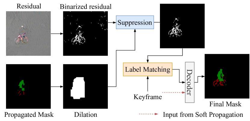
Figure 5: Residual-based correction module selects pixels to correct in the propagated mask; the correction scheme replaces the segmentation labels via a feature matching scheme.

4.4 Keyframe & base network selection

In principle, any frame can be a keyframe. However, it is natural to define keyframes according to the compressed frame type, as the encoder designates types based on the video’s dynamic content. In addition to I-frames, we also choose P-frames as keyframes. This is because less than 5% of frames in a video sequence are I-frames in the default HEVC encoding, which is insufficient for accurate propagation, so we also include the 15-35% of frames designated as P-frames. Considering P-frames as keyframes also helps improve the accuracy because the motion compensation in P-frames is strictly uni-directional. Otherwise, propagation to these frames may suffer inaccuracies arising from occlusions in the same manner as optical flow.

For a base VOS model to be accelerated, most matching based segmentation models discussed in  Sec. 2 are suitable as they rely only on the appearance of the target object. From preliminary experiments, we observed that VOS methods that use memory-networks such as STM [20], MiVOS [4], and STCN [5] are ideal for acceleration. This is because the choice of using I- and P-frames as keyframes naturally aligns with the memory concept and allows for the selection of a (even more) compact yet diverse memory.

Table 1: Comparison of acceleration on different base models with state-of-the-art methods. †Frame rates were measured on our device if originally not provided; we also re-estimated STM time on our hardware as we obtained higher FPS than their reported value. FPS on Youtube-VOS is measured on the first 30 videos.

	DAVIS16 validation				DAVIS17 validation				YouTube-VOS 2018 validation
Method	$\mathcal{J}$	$\mathcal{F}$	$\mathcal{J}\&\mathcal{F}$	FPS	$\mathcal{J}$	$\mathcal{F}$	$\mathcal{J}\&\mathcal{F}$	FPS	$\mathcal{G}$	$\mathcal{J}_{s}$	$\mathcal{F}_{s}$	$\mathcal{J}_{u}$	$\mathcal{F}_{u}$	FPS
CVOS[32]	79.1	80.3	79.7	34.5	57.4	59.3	58.4	31.2	-	-	-	-	-	-
TVOS[44]	-	-	-	-	69.9	74.7	72.3	37	67.8	67.1	69.4	63.0	71.6	-
Track-Seg[3]	82.6	83.6	83.1	39	68.6	76.0	72.3	$<$39	63.6	67.1	70.2	55.3	61.7	-
PReMVOS [17]	84.9	88.6	86.8	0.03	73.9	81.7	77.8	$<$0.03	66.9	71.4	75.9	56.5	63.7	-
SwiftNet [36]	90.5	90.3	90.4	25	78.3	83.9	81.1	25	77.8	77.8	81.8	72.3	79.5	-
CFBI+ [43]	88.7	91.1	89.9	5.6	80.1	85.7	82.9	$<$5.6	82.0	81.2	86.0	76.2	84.6	-
FRTM-VOS [27]	-	-	83.5	21.9	-	-	76.7	†14.1	72.1	72.3	76.2	65.9	74.1	†7.7
FRTM-VOS + CoVOS	82.3	82.2	82.3	28.6	69.7	75.2	72.5	20.6	65.6	68.0	71.0	58.2	65.4	25.3
STM [20]	88.7	89.9	89.3	†14.9	79.2	84.3	81.8	†10.6	79.4	79.7	84.2	72.8	80.9	-
STM + CoVOS	87.0	87.3	87.2	31.5	78.3	82.7	80.5	23.8	-	-	-	-	-	-
MiVOS [4]	89.7	92.4	91.0	16.9	81.7	87.4	84.5	11.2	82.6	81.1	85.6	77.7	86.2	†13
MiVOS + CoVOS	89.0	89.8	89.4	36.8	79.7	84.6	82.2	25.5	79.3	78.9	83.0	73.5	81.7	45.9
STCN [5]	90.4	93.0	91.7	26.9	82.0	88.6	85.3	20.2	84.3	83.2	87.9	79.0	87.3	†16.8
STCN + CoVOS	88.5	89.6	89.1	42.7	79.7	85.1	82.4	33.7	79.0	79.4	83.6	72.6	80.4	57.9

5 Experimentation

5.1 Experimental settings

Video Compression. We generated compressed video from images using the x265 library in FFmpeg on the default preset. To write out the bitstream, we modified the decoder from openHEVC[9, 8] and shared the code publicly to encourage others to work with compressed video.

Datasets & Evaluation. We experimented with three video object segmentation benchmarks: DAVIS16[24] and DAVIS17[25], which are small datasets with 50 and 120 videos of single and multiple objects, respectively, and YouTube-VOS[42], a large-scale dataset with 3945 videos of multiple objects. We used the images in their original resolution for encoding the videos. The default HEVC encoding produced an average of {37%, 36%, 27%} of I/P-frames, and therefore keyframes per sequence for DAVIS16, DAVIS17 and YouTube-VOS, respectively.

We evaluated with the standard criteria from [24]: Jaccard Index $\mathcal{J}$ (IoU of the output segmentation with ground-truth mask) for region similarity, and mean boundary $\mathcal{F}$-scores for contour accuracy. Additionally, we report the average over all seen and unseen classes for YouTube-VOS.

Propagation & Correction. In our propagation scheme, we applied reverse mapping for warping and nearest-neighbour interpolation kernels. The decoder in the soft propagation (Sec. 4.2) is a lightweight network of three residual blocks (see Supplementary for details). The decoder is trained from scratch, with a uniform initialization and a learning rate of 1e-4 with a decay factor of 0.1 every 10k iterations for 40k iterations. For residual-based correction, the binary threshold was set to $0.15\!*\!255$ for the absolute value of gray-scaled residual.

Base Models. We show experiments accelerating four base models: STM [20], MiVOS [4], STCN [4] and FRTM-VOS [27]. The first three use a memory bank; for a fair comparison, we allow only keyframes to be stored in the memory bank. We set the memory frequency to 2 on DAVIS and 5 on Youtube-VOS, as the latter has higher frame rates. In the experiments, both settings reduced the memory bank size. We refer to Supplementary for the memory analysis. FRTM-VOS fine-tunes a network based on the labelled frame and associated augmentations. We fed only the keyframes into the network for segmentation and fine-tuning. In practice, this is equivalent to segmenting a temporally reduced video.

5.2 Acceleration on different base models.

Tab. 1 compares our accelerated results on the four base models with other state-of-the-art models. Our method achieves an excellent compromise between accuracy and speed. On DAVIS16 ($\approx\!37\%\!$ keyframes), we achieved $1.3\times$, $2.1\times$, $2.2\times$, $1.6\times$ speed-ups with a minor drop of $\mathcal{J}\&\mathcal{F}$ $1.2$, $2.1$, $1.6$, $2.6$ on FRTM-VOS, STM, MiVOS and STCN, respectively. On DAVIS17 ($\approx 36\%\!$ keyframes), we achieved $1.5\times$, $2.2\times$, $2.3\times$, $1.7\times$ speed-ups with the drop on $\mathcal{J}\&\mathcal{F}$ $4.2$, $1.3$, $1.7$, $2.9$ for the same order of models.

On YouTube-VOS ($\approx\!27\%\!$ keyframes), we achieved $3.3\times$, $3.5\times$, $3.4\times$ speed-ups with a $4.8$, $2.4$, $4.0$ drop of $\mathcal{J}_{s}\&\mathcal{F}_{s}$ for FRTM-VOS, MiVOS and STCN, respectively. We have larger drops on $\mathcal{J}_{u}\&\mathcal{F}_{u}$ for unseen data because our decoder is not pre-trained on larger datasets. Note that the video lengths of YouTube-VOS are relatively long ($>$150frames), so the above methods require additional memory or additional online fine-tuning, which allows us to achieve higher speed-ups. Moreover, the lower keyframe percentage of YouTube-VOS also provides more speed-ups. We do not provide the result on STM as no pre-trained weights are available.

With an STCN base model, our performance on DAVIS17 is 1.3 to 10.1 higher than other efficient methods SwiftNet [36], TVOS [44] and Track-Seg [3] with comparable frame rates, though our success should also be attributed to the high STCN base accuracy. Another compressed video method CVOS [32] achieves comparable speed but has a significant accuracy gap.

5.3 Ablation studies

We verified each component of our framework. All ablations used MiVOS[4] as the base model on default video encode preset unless otherwise indicated.

Propagation. We first compare with optical flow as a form of propagation, and consider a forward unidirectional flow warping as done in [7, 23, 45], using the flow from the state-of-the-art method RAFT [33] (‘Optical Flow’). We also consider a bi-directional optical flow warping (‘Bi-Optical Flow’), which is used in [21]. Additionally, we compare with two motion vector baselines from a work on compressed videos, CoViAR [40] (‘MV to Flow’), and another work on compressed VOS, CVOS [32] (‘MV I to P’). CoViAR converts motion vectors into a flow between two frames, i.e. for motion vector field $M_{i}$ at $(x,y)$ and frame $i$, $M_{of}(x,y)=[u,v]/[(t-i)\cdot fps]$ is the motion of the pixel $(x,y)$ in the unit time on plane $i$. CVOS has a further simplified motion vector usage and references all motions from one I-frame in the GOP. We compare our bi-directional, multi-hop motion vector warping with (‘MV Soft Prop’) and without (‘MV Warp’) the soft propagation, which performs further noise suppression.

Table 2: Comparison of propagation methods, ’B’, ’M’, ’Sup’ denotes bi-directional, multi-hop and noise suppression, respectively. ^†No code given, we report the results from earlier work [32]

				DAVIS16		DAVIS17
Method	B	M	Sup	$\mathcal{J}$	$\mathcal{F}$	$\mathcal{J}$	$\mathcal{F}$
Optical Flow				77.4	79.2	71.5	77.6
Bi-Optical Flow [21]	✗			85.0	87.4	75.9	81.7
MV I to P [32]				31.5†	-	-	-
MV to Flow [40]				77.2	80.2	69.4	76.3
MV Warp	✗	✗		85.7	89.2	77.2	84.4
MV Soft Prop	✗	✗	✗	89.0	89.8	79.7	84.6
No propagation [4]				89.7	92.4	81.7	87.4

Tab. 2 verifies the effectiveness of our proposed propagation. Bi-directional optical flow, originally used for video generation [21], performs better than unidirectional optical flow because it is less affected by occlusion. CoViAR [40] is a compressed video action recognition system; their propagation is on par with optical flow. The simplified case in CVOS [32] fails to propagate meaningful segmentation masks and thus relies on heavy refinement.

Our bi-directional multi-hop motion vector-based warping outperforms all of the above methods. Our soft propagation scheme with noise suppression gives further improvements to the accuracy, such that our propagated masks are within 4.0 points on both $\mathcal{J}$ and $\mathcal{F}$ below the upper bound without propagation, i.e. by applying each frame through the base network. Fig. 6 shows qualitative results on different propagation methods.

Table 3: Ablations on decoder and mask correction module.

	DAVIS16		DAVIS17
Module	$\mathcal{J}$	$\mathcal{F}$	$\mathcal{J}$	$\mathcal{F}$
MV Warp	85.7	89.2	77.2	84.4
+Decoder	88.3	88.8	79.2	84.0
+Suppression	88.8	89.6	79.6	84.5
+Residual Correction	89.0	89.8	79.7	84.6

Decoder and mask correction. Tab. 3 shows how adding each component of the mask decoder leads to progressive improvements for the $\mathcal{J}$-index and boundary $\mathcal{F}$-score. For ‘MV Warp’, we directly warp the prediction results on the original size of the frame. For the decoder, we warp the prediction and low-level features at 1/4 size for speed consideration. Because the motion vector is coarse and noisy, only input propagated prediction and the low-level features to the decoder will decrease accuracy. The most significant gains come from the noise suppression module, i.e. by feeding the suppressed propagated prediction into the decoder. Further residual correction increases the robustness for the corner cases.

Keyframe percentage. To highlight the speed-accuracy trade-off, we compare the percentage of keyframes in Tab. 4 by adjusting encoder presets. The default HEVC setting yields $\approx 37\%$ keyframes for DAVIS16 and DAVIS17. If we set the encoder to allocate more B-frames to have only approximately $25\%$ and $13\%$ keyframes (‘B-frame biased’ and ‘Uniform B-frames’, respectively), the propagated scores decrease while the FPS values increase accordingly. At the fastest setting, we can achieve 3.7x speed-ups on MiVOS with $\mathcal{J}\&\mathcal{F}$ scores of 82.9 on DAVIS16 and 4.5x speed-ups with $\mathcal{J}\&\mathcal{F}$ scores of 73.2 on DAVIS17.

Table 4: Robustness to different video encoding presets on DAVIS16 and DAVIS17. B-frame biased: more weight on B-frame allocation (x265 option: bframe-bias=50). Uniform B-frames: fixed 8 B-frames between I/P frames.

		DAVIS16		DAVIS17
Preset	Keyframe	$\mathcal{J}\&\mathcal{F}$	FPS	$\mathcal{J}\&\mathcal{F}$	FPS
Default	$\approx 37\%$	89.4	36.8	82.2	25.5
B-frame biased	$\approx 25\%$	85.1	48.2	80.2	36.7
Uniform B-frames	$\approx 13\%$	82.9	62.9	73.2	50.0
No Propagation	-	91.0	16.9	84.5	11.2

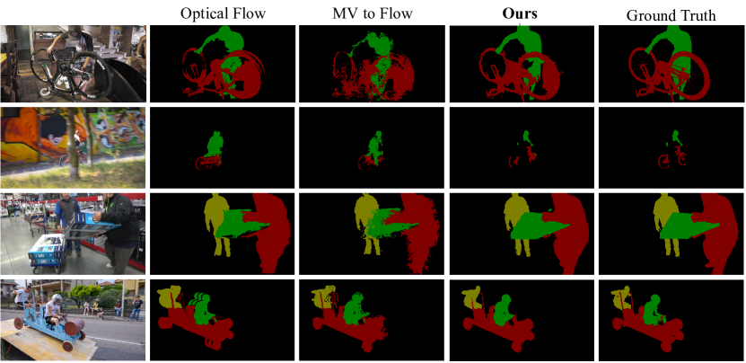
Figure 6: Optical flow propagation and motion-vector generated flows both suffer from ghosting effects and holes in areas of occlusion. Our propagation successfully prevents such artifacts.

5.4 Timing analysis

To compute the FPS values in all our tables, we measured run times on an RTX-2080Ti for DAVIS dataset and on an RTX-A5000 for YouTube-VOS, as it requires extra memory. The amortized per frame inference time can be approximately computed by $T_{\text{base}}\!\cdot\!R\!+\!(T_{\text{propagation}}+\!T_{\text{correction}})\!\cdot\!(1\!-\!R)$, where $R$ denotes the ratio of keyframes. Note that the measured $T_{\text{base}}$ may not correspond to the published FPS values of the base model, e.g. for STM[20] and MiVOS[4]. Our $T_{\text{base}}$ is lower because we store fewer frames in the memory bank (see Supplementary for more details). We measured the propagation and correction time on DAVIS17, and the sum ($T_{\text{propagation}}\!+\!T_{\text{correction}}$) is $12$ms.

6 Conclusion & limitations

We propose an acceleration framework for semi-supervised VOS via propagation by exploiting the motion vectors and residuals of the compressed video bitstream. Such a framework can speed up the accurate but slow base VOS models with minor drops in segmentation accuracy. One limitation of our work is the possible latency introduced by the multiple reference dependencies. As a result, segmentation results of a non-keyframe get completed later than the future frame to which it refers.

Given that 70% of the internet traffic [12] is dedicated to (compressed) videos, we see broad applicability of our work for acceleration. Efficiency in VOS methods is especially relevant for applications such as video editing, given the growing trend of higher resolution videos, e.g.  4K standards. However, VOS could also be abused to falsify parts of videos or create malicious content. We maintain a rigorous attitude towards this while emphasizing its positive impact on content creation and other possible improvements for the community.

7 Acknowledgements

This research is supported by the National Research Foundation, Singapore under its NRF Fellowship for AI (NRF-NRFFAI1-2019-0001). Any opinions, findings and conclusions or recommendations expressed in this material are those of the author(s) and do not reflect the views of National Research Foundation, Singapore.

References

- [1] R Venkatesh Babu, KR Ramakrishnan, and SH Srinivasan. Video object segmentation: a compressed domain approach. TCSTV, 2004.
- [2] Sergi Caelles, Kevis-Kokitsi Maninis, Jordi Pont-Tuset, Laura Leal-Taixé, Daniel Cremers, and Luc Van Gool. One-shot video object segmentation. In CVPR, 2017.
- [3] Xi Chen, Zuoxin Li, Ye Yuan, Gang Yu, Jianxin Shen, and Donglian Qi. State-aware tracker for real-time video object segmentation. In CVPR, 2020.
- [4] Ho Kei Cheng, Yu-Wing Tai, and Chi-Keung Tang. Modular interactive video object segmentation: Interaction-to-mask, propagation and difference-aware fusion. In CVPR, 2021.
- [5] Ho Kei Cheng, Yu-Wing Tai, and Chi-Keung Tang. Rethinking space-time networks with improved memory coverage for efficient video object segmentation. In NeurIPS, 2021.
- [6] Jingchun Cheng, Yi-Hsuan Tsai, Shengjin Wang, and Ming-Hsuan Yang. Segflow: Joint learning for video object segmentation and optical flow. In ICCV, 2017.
- [7] Alexey Dosovitskiy, Philipp Fischer, Eddy Ilg, Philip Hausser, Caner Hazirbas, Vladimir Golkov, Patrick Van Der Smagt, Daniel Cremers, and Thomas Brox. Flownet: Learning optical flow with convolutional networks. In ICCV, 2015.
- [8] Wassim Hamidouche, Michael Raulet, and Olivier Déforges. Parallel shvc decoder: Implementation and analysis. In ICME, 2014.
- [9] Wassim Hamidouche, Michael Raulet, and Olivier Déforges. Real time shvc decoder: Implementation and complexity analysis. In ICIP, 2014.
- [10] Ping Hu, Gang Wang, Xiangfei Kong, Jason Kuen, and Yap-Peng Tan. Motion-guided cascaded refinement network for video object segmentation. In CVPR, 2018.
- [11] Eddy Ilg, Nikolaus Mayer, Tonmoy Saikia, Margret Keuper, Alexey Dosovitskiy, and Thomas Brox. Flownet 2.0: Evolution of optical flow estimation with deep networks. In CVPR, 2017.
- [12] Cisco Visual Networking Index. Forecast and methodology, 2016–2021. White paper, Cisco public, 2017.
- [13] Samvit Jain, Xin Wang, and Joseph Gonzalez. Accel: A corrective fusion network for efficient semantic segmentation on video. In CVPR, 2019.
- [14] Didier Le Gall. Mpeg: A video compression standard for multimedia applications. Communications of the ACM, 1991.
- [15] Yong Jae Lee, Jaechul Kim, and Kristen Grauman. Key-segments for video object segmentation. In ICCV, 2011.
- [16] Yule Li, Jianping Shi, and Dahua Lin. Low-latency video semantic segmentation. In CVPR, 2018.
- [17] Jonathon Luiten, Paul Voigtlaender, and Bastian Leibe. Premvos: Proposal-generation, refinement and merging for video object segmentation. In ACCV, 2018.
- [18] Kevis-Kokitsi Maninis, Sergi Caelles, Yuhua Chen, Jordi Pont-Tuset, Laura Leal-Taixé, Daniel Cremers, and Luc Van Gool. Video object segmentation without temporal information. TPAMI, 2017.
- [19] Seoung Wug Oh, Joon-Young Lee, Kalyan Sunkavalli, and Seon Joo Kim. Fast video object segmentation by reference-guided mask propagation. In CVPR, 2018.
- [20] Seoung Wug Oh, Joon-Young Lee, Ning Xu, and Seon Joo Kim. Video object segmentation using space-time memory networks. In ICCV, 2019.
- [21] Junting Pan, Chengyu Wang, Xu Jia, Jing Shao, Lu Sheng, Junjie Yan, and Xiaogang Wang. Video generation from single semantic label map. In CVPR, 2019.
- [22] Matthieu Paul, Christoph Mayer, Luc Van Gool, and Radu Timofte. Efficient video semantic segmentation with labels propagation and refinement. In WACV, 2020.
- [23] Federico Perazzi, Anna Khoreva, Rodrigo Benenson, Bernt Schiele, and Alexander Sorkine-Hornung. Learning video object segmentation from static images. In CVPR, 2017.
- [24] F. Perazzi, J. Pont-Tuset, B. McWilliams, L. Van Gool, M. Gross, and A. Sorkine-Hornung. A benchmark dataset and evaluation methodology for video object segmentation. In CVPR, 2016.
- [25] Jordi Pont-Tuset, Federico Perazzi, Sergi Caelles, Pablo Arbeláez, Alexander Sorkine-Hornung, and Luc Van Gool. The 2017 davis challenge on video object segmentation. arXiv:1704.00675, 2017.
- [26] Fatih Porikli, Faisal Bashir, and Huifang Sun. Compressed domain video object segmentation. TCSVT, 2009.
- [27] Andreas Robinson, Felix Jaremo Lawin, Martin Danelljan, Fahad Shahbaz Khan, and Michael Felsberg. Learning fast and robust target models for video object segmentation. In CVPR, 2020.
- [28] Hongje Seong, Junhyuk Hyun, and Euntai Kim. Kernelized memory network for video object segmentation. In ECCV, 2020.
- [29] Thomas Sikora. The mpeg-4 video standard verification model. TCSVT, 1997.
- [30] Gary J. Sullivan, Jens-Rainer Ohm, Woo-Jin Han, and Thomas Wiegand. Overview of the high efficiency video coding (hevc) standard. TCSTV, 2012.
- [31] Vivienne Sze, Madhukar Budagavi, and Gary J Sullivan. High efficiency video coding (hevc). In Integrated circuit and systems, algorithms and architectures. 2014.
- [32] Zhentao Tan, Bin Liu, Qi Chu, Hangshi Zhong, Yue Wu, Weihai Li, and Nenghai Yu. Real time video object segmentation in compressed domain. TCSVT, 2020.
- [33] Zachary Teed and Jia Deng. Raft: Recurrent all-pairs field transforms for optical flow. In ECCV, 2020.
- [34] David Tsai, Matthew Flagg, Atsushi Nakazawa, and James M Rehg. Motion coherent tracking using multi-label mrf optimization. IJCV, 2012.
- [35] Paul Voigtlaender and Bastian Leibe. Online adaptation of convolutional neural networks for video object segmentation. arXiv:1706.09364, 2017.
- [36] Haochen Wang, Xiaolong Jiang, Haibing Ren, Yao Hu, and Song Bai. Swiftnet: Real-time video object segmentation. In CVPR, 2021.
- [37] Qiang Wang, Li Zhang, Luca Bertinetto, Weiming Hu, and Philip HS Torr. Fast online object tracking and segmentation: A unifying approach. In CVPR, 2019.
- [38] Shiyao Wang, Hongchao Lu, and Zhidong Deng. Fast object detection in compressed video. In ICCV, 2019.
- [39] Thomas Wiegand, Gary J Sullivan, Gisle Bjontegaard, and Ajay Luthra. Overview of the h. 264/avc video coding standard. TCSVT, 2003.
- [40] Chao-Yuan Wu, Manzil Zaheer, Hexiang Hu, R Manmatha, Alexander J Smola, and Philipp Krähenbühl. Compressed video action recognition. In CVPR, 2018.
- [41] Mai Xu, Lai Jiang, Xiaoyan Sun, Zhaoting Ye, and Zulin Wang. Learning to detect video saliency with hevc features. TIP, 2017.
- [42] Ning Xu, Linjie Yang, Yuchen Fan, Dingcheng Yue, Yuchen Liang, Jianchao Yang, and Thomas Huang. Youtube-vos: A large-scale video object segmentation benchmark. arXiv:1809.03327, 2018.
- [43] Zongxin Yang, Yunchao Wei, and Yi Yang. Collaborative video object segmentation by multi-scale foreground-background integration. TPAMI, 2021.
- [44] Yizhuo Zhang, Zhirong Wu, Houwen Peng, and Stephen Lin. A transductive approach for video object segmentation. In CVPR, 2020.
- [45] Xizhou Zhu, Yuwen Xiong, Jifeng Dai, Lu Yuan, and Yichen Wei. Deep feature flow for video recognition. In CVPR, 2017.