Scalarized Einstein-Maxwell-scalar Black Holes in a Cavity

Abstract

In this paper, we study the spontaneous scalarization of Reissner-Nordström (RN) black holes enclosed by a cavity in an Einstein-Maxwell-scalar (EMS) model with non-minimal couplings between the scalar and Maxwell fields. In this model, scalar-free RN black holes in a cavity may induce scalarized black holes due to the presence of a tachyonic instability of the scalar field near the event horizon. We calculate numerically the black hole solutions, and investigate the domain of existence, perturbative stability against spherical perturbations and phase structure. The scalarized solutions are always thermodynamically preferred over RN black holes in a cavity. In addition, a reentrant phase transition, composed of a zeroth-order phase transition and a second-order one, occurs for large enough electric charge $Q$.

I Introduction

The no-hair theorem is important to understand black hole physics, which initially states that all black hole can be uniquely characterized by only three externally observable parameters: mass, electric charge, and angular momentum. Although the no-hair theorem has been proven for the Einstein-Maxwell field theory, the advent of hairy black hole solutions in the context of the Einstein-Yang-Mills theory Volkov:1989fi ; Bizon:1990sr prompt people to reconsider the no-hair theorem. Later, black holes with Skyrme hairs Luckock:1986tr ; Droz:1991cx and black holes with dilaton hairs Kanti:1995vq were also discovered as counter-examples to the no-hair theorem. For a recent review, see Herdeiro:2015waa .

As a way of formation of hairy black holes, spontaneous scalarization is first studied for neutron stars in scalar-tensor models Damour:1993hw . In this phenomenon of spontaneous scalarization, the non-minimal coupling of the scalar field to the Ricci curvature can lead to a certain parameter region, where scalar-free and scalarized neutron star solutions coexist, and the scalarized one is energetically favoured. Later, the spontaneous scalarization of black holes is also found in scalar-tensor models Cardoso:2013opa ; Cardoso:2013fwa . Recently, the authors of Doneva:2017bvd ; Silva:2017uqg ; Antoniou:2017acq ; Doneva:2018rou ; Cunha:2019dwb ; Herdeiro:2020wei studied the spontaneous scalarization in the extended Scalar-Tensor-Gauss-Bonnet (eSTGB) gravity, where the scalar field is non-minimally coupled to the Gauss-Bonnet curvature invariant of the gravitational sector. However, the numerical challenges of studying dynamical evolution equations in this model compels people to consider other simpler model. It is at this juncture that the Einstein-Maxwell-scalar (EMS) models were introduced to gain a deeper insight into spontaneous scalarization Herdeiro:2018wub . In these models, spontaneous scalarization can be triggered by the strong non-minimal coupling of the scalar field to the electromagnetic field. In Herdeiro:2018wub , a massless and non-self-interacting scalar field was considered, and an exponential coupling function was introduced to ensure a tachyonic instability of Reissner-Nordström (RN) black holes. In Hod:2020cal , the analytical technique is applyied to solve the Klein–Gordon wave equation for the non-minimally coupled linearized scalar fields in the spacetimes of near-extremal supporting black holes. Furthermore, spontaneous scalarization in the EMS models was discussed in context of coupling functions beyond the exponential coupling Fernandes:2019rez ; Blazquez-Salcedo:2020nhs , dyons including magnetic charges Astefanesei:2019pfq , axionic-type couplings Fernandes:2019kmh , massive and self-interacting scalar fields Zou:2019bpt ; Fernandes:2020gay , horizonless reflecting stars Peng:2019cmm , linear stability of scalarized black holes Myung:2018vug ; Myung:2019oua ; Zou:2020zxq , higher dimensional scenario Astefanesei:2020qxk , quasinormal modes of scalarized black holes Myung:2018jvi ; Blazquez-Salcedo:2020jee , two U(1) fields Myung:2020dqt and quasi-topological electromagnetism Myung:2020ctt . Moreover, the EMS models with a cosmological constant are considered in Brihaye:2019gla ; Guo:2021zed . Recently, the effect of Non-linear electrodynamics corrections on the EMS models is also studied Wang:2020ohb . Analytic approximations were also used to study spontaneous scalarization of the EMS models Konoplya:2019goy ; Hod:2020ljo ; Hod:2020ius .

Over the past four decades a preponderance of evidence has accumulated suggesting a fundamental relationship between gravitation, thermodynamics, and quantum theory. This evidence is rooted in our understanding of black holes and their relationship to quantum physics, and developed into the sub-discipline of black hole thermodynamics. Since the discover of the area theorem Hawking:1971tu and the Hawking radiation Hawking:1974rv ; Hawking:1974sw , the analogy between usual thermodynamics and black hole thermodynamics is confirmed. Furthermore, the four laws of black hole mechanics were established in Bardeen:1973gs and numerous studies have focused on this subject. Since it is shown that asymptotically anti-de Sitter (AdS) black holes are thermodynamically stable and the Hawking-Page phase transition was revealed in Schwarzschild-AdS black holes Hawking:1982dh , thermodynamic properties of various more complicated black holes have been studied Witten:1998zw ; Cvetic:1999ne ; Chamblin:1999tk ; Chamblin:1999hg ; Caldarelli:1999xj ; Cai:2001dz ; Cvetic:2001bk ; Nojiri:2001aj

As parallel research with that of AdS black holes, studies of black holes in a cavity have also attracted a lot attentions since York realized that Schwarzschild black holes can be thermally stable by placing them inside a spherical cavity, on the wall of which the metric is fixed York:1986it . The phase structure and transitions of black holes in a cavity were shown to closely resemble that of the AdS counterparts for Schwarzschild black holes York:1986it and RN black holes Braden:1990hw ; Carlip:2003ne ; Lundgren:2006kt . Recently, it is found that the resemblance still exist in the extended phase space Wang:2020hjw . And it was discovered that Gauss-Bonnet black holes in a cavity also have quite similar phase structure and transitions to the AdS counterparts Wang:2019urm . However, it is shown that the phase structure of Born-Infeld black holes enclosed in a cavity has dissimilarities from that of Born-Infeld-AdS black holes Wang:2019kxp ; Liang:2019dni . Moreover, it is found that there exist significant differences between the thermodynamic geometry of RN black holes in a cavity and that of RN-AdS black holes Wang:2019cax , and some dissimilarities between the two cases also occur for validities of the second thermodynamic law and the weak cosmic censorship Wang:2020osg . These findings motivate us to further explore connections between thermodynamic properties of black holes and their boundary conditions. For black holes in a cavity, it is shown that there exist the black hole bomb setup for Kerr black holes Press:1972zz ; Cardoso:2004nk . Although it is shown the black hole bomb still exists for charged black holes in a cavity Herdeiro:2013pia ; Hod:2013fvl ; Dias:2018zjg , the hairy black holes in a cavity are also found for Einstein-Maxwell gravity coupled to a charged scalar field Dias:2018yey . Therefore, it is interesting to investigated hairy black holes in a cavity for the EMS model and compare the results with those of AdS case Guo:2021zed .

Nevertheless, the solutions and thermodynamics of hairy black holes in cavity have rarely been studied in the context of the EMS model. The rest of this paper is organized as follows. Section II presents the basics of the EMS model and provides the equations of motion for the solution ansatz of interest. In section III, we review the scalar-free RN black holes in cavity and show our main numerical results for scalarized black hole solutions in a cavity, which include domains of existence, thermodynamic preference and effective potentials for radial perturbations. In section IV, we discuss the phase structure and transitions in a canonical ensemble. We summarize our results with a brief discussion in section V. For simplicity, we set $16\pi G=1$ in this paper.

II EMS Model in a Cavity

The EMS model describes a real scalar field minimally coupled to Einstein’s gravity and non-minimally coupled to Maxwell’s electromagnetism. In a cavity, the EMS model is described by the action

$$\mathcal{S=}\int_{\mathcal{M}}d^{4}x\sqrt{-g}\left[R-2\partial_{\mu}\phi\partial^{\mu}\phi-f\left(\phi\right)F^{\mu\nu}F_{\mu\nu}\right]+\mathcal{S}_{surf},$$ (1)

where $f\left(\phi\right)$ is the coupling function governing the non-minimal coupling of $\phi$ and $A_{\mu}$, $F_{\mu\nu}=\partial_{\mu}A_{\nu}-\partial_{\nu}A_{\mu}$ is the electromagnetic field strength tensor. And $\mathcal{S}_{surf}$ is the surface terms on $\partial\mathcal{M}$, which does not affect the equations of motion. Therefore, the equations of motion that follow from the action $\left(\ref{eq:IS}\right)$ are

$$R_{\mu\nu}-\frac{1}{2}Rg_{\mu\nu} =\frac{\mathcal{T}_{\mu\nu}}{2},$$

$$\partial_{\mu}\left[\sqrt{-g}f\left(\phi\right)F^{\mu\nu}\right] =0,$$ (2)

$$\frac{\partial^{\mu}\left(\sqrt{-g}\partial_{\mu}\phi\right)}{\sqrt{-g}} =\frac{\dot{f}\left(\phi\right)F^{\mu\nu}F_{\mu\nu}}{4},$$

where $\dot{f}\left(\phi\right)\equiv df\left(\phi\right)/d\phi$, and the energy-momentum tensor is

$$\mathcal{T}_{\mu\nu}=4\left(\partial_{\mu}\phi\partial_{\nu}\phi-\frac{g_{\mu\nu}\partial_{\rho}\phi\partial^{\rho}\phi}{2}\right)+f\left(\phi\right)\left[4F_{\mu\rho}F_{\nu}^{\text{ }\rho}-F^{\mu\nu}F_{\mu\nu}\right].$$ (3)

The generic spherically symmetric metric can be written as

$$ds^{2}=-N\left(r\right)e^{-2\delta\left(r\right)}dt^{2}+\frac{dr^{2}}{N\left(r\right)}+r^{2}\left(d\theta^{2}+\sin^{2}\theta d\varphi^{2}\right),$$ (4)

The electromagnetic field and the scalar field are given by $A_{\mu}dx^{\mu}=V\left(r\right)dt$ and $\phi=\phi\left(r\right)$, respectively. Then the equations of motion $\left(\ref{eq:IEOM}\right)$ reduce to

$$-1+N\left(r\right)+rN^{\prime}\left(r\right)+r^{2}N\left(r\right)\phi^{\prime}\left(r\right) =-\frac{Q^{2}}{r^{2}f\left(\phi\right)},$$

$$\left[r^{2}N\left(r\right)\phi^{\prime}\left(r\right)\right]^{\prime}+r^{3}\phi^{\prime}\left(r\right)^{3}N\left(r\right) =-\frac{Q^{2}\dot{f}\left(\phi\right)}{2f^{2}\left(\phi\right)r^{2}},$$

$$\delta^{\prime}\left(r\right) =-r\phi^{\prime}\left(r\right)^{2},$$ (5)

$$V^{\prime}\left(r\right) =-\frac{e^{-\delta\left(r\right)}Q}{r^{2}f\left(\phi\right)},$$

where primes denote derivatives with respect to the radial coordinate $r$, and $Q$ is a constant that can be interpreted as the electric charge.

III Scalarized RN Black Hole in a Cavity

In this paper, we study spontaneous scalarization of the EMS model in a cavity, which requires a scalar-free solution. When the scalar field $\phi=0$, the static spherically symmetric RN black hole solution was derived in Braden:1990hw ,

$$N\left(r\right)=\left(1-\frac{r_{+}}{r}\right)\left(1-\frac{Q_{b}^{2}}{r_{+}r}\right)\equiv 1-\frac{2m(r)}{r},\text{ }V\left(r\right)=-\frac{Q_{b}}{r}dt,\text{ }\delta\left(r\right)=0,$$ (6)

where $Q_{b}$ is the black hole charge, and $r_{+}$ is the radius of the outer event horizon. The Hawking temperature $T_{b}$ of the RN black hole is given by

$$T_{b}=\frac{1}{4\pi r_{+}}\left(1-\frac{Q_{b}^{2}}{r_{+}^{2}}\right).$$ (7)

In this scalar-free solution background, one can linearize the scalar equation in eqn. $\left(\ref{eq:IEOM}\right)$ around the scalar-free solution, which gives

$$\frac{\partial^{\mu}\left(\sqrt{-g}\partial_{\mu}\delta\phi\right)}{\sqrt{-g}}=\mu_{eff}^{2}\text{ },$$ (8)

where $\mu_{eff}^{2}=-\ddot{f}\left(0\right)Q^{2}/\left(2r^{4}\right)$. If $\mu_{eff}^{2}<0$, i.e. $\ddot{f}\left(0\right)>0$, a tachyonic instability is induced, and a scalarized black hole solution can bifurcate from the scalar-free RN black hole solution. In the remainder of the paper, we focus an exponential coupling, $f\left(\phi\right)=e^{\alpha\phi^{2}}$ with $\alpha>0$, which satisfies $\dot{f}\left(0\right)=0$ and $\ddot{f}\left(0\right)>0$.

To obtain non-trivial hairy black hole solutions of the non-linear ordinary differential equations $\left(\ref{eq:EoM}\right)$, one needs to impose regular boundary conditions at the event horizon and the boundary of the cavity. The regularity of the solutions across the event horizon at $r=r_{+}$ gives that the solutions can be approximated by a power series expansion in $r-r_{+}$,

$$m\left(r\right) =\frac{r_{+}}{2}+\left(r-r_{+}\right)m_{1}+...\text{, }\delta\left(r\right)=\delta_{0}+\left(r-r_{+}\right)\delta_{1}+...,$$

$$\phi\left(r\right) =\phi_{0}+\left(r-r_{+}\right)\phi_{1}+...\text{, }V\left(r\right)=\left(r-r_{+}\right)v_{1}+...\text{, }$$ (9)

where

$$m_{1}=\frac{Q^{2}}{2r_{+}^{2}f\left(\phi_{0}\right)},\text{ }\phi_{1}=-\frac{Q^{2}\dot{f}\left(\phi_{0}\right)}{2\left[f^{2}\left(\phi_{0}\right)r_{+}^{3}-f\left(\phi_{0}\right)r_{+}Q^{2}\right]},\text{ }\delta_{1}=-r_{+}\phi_{1}^{2},\text{ }v_{1}=\frac{Qe^{-\delta_{0}}}{r_{+}^{2}f\left(\phi_{0}\right)}.$$ (10)

The parameters $\phi_{0}$ and $\delta_{0}$ determine the expansion coefficients and hence the solutions in the vicinity of the horizon. Outside the cavity, we require that the scalar field vanishes and it recover the scalar-free solution Dias:2018yey . Therefore the boundary conditions at the boundary of the cavity is

$$\phi\left(r_{B}\right)=0,\delta\left(r_{B}\right)=0.$$

We can use a standard shooting method to solve eqn. $\left(\ref{eq:EoM}\right)$ for a family of black hole solutions with the boundary conditions at the event horizon and the boundary of the cavity. Note that the solutions and the associated physical quantities scale as

$$r\rightarrow\lambda r,\phi\rightarrow\phi,m\rightarrow\lambda m,V\rightarrow V,\delta\rightarrow\delta,Q\rightarrow\lambda Q,M\rightarrow\lambda M,$$ (11)

where $\lambda$ is a constant and the ADM mass $M$ is introduced by the asymptotic expansion of the solutions at spatial infinity,

$$m\left(r\right)=M-\frac{Q^{2}+Q_{s}^{2}}{2r}+...,$$ (12)

.So we introduce some reduced quantities for later use,

$$q=\frac{Q}{M},a_{H}=\frac{A_{H}}{16\pi M^{2}},t_{H}=8\pi MT_{H},$$ (13)

which are dimensionless and invariant under the scaling symmetry.

To study how a scalarized black hole solution bifurcates from a scalar-free solution, we derive the zero modes of the scalar perturbation in the scalar-free black hole background. First, we express the scalar perturbation as a spherical harmonics decomposition

$$\delta\phi={\displaystyle\sum\limits_{l,m}}Y_{lm}\left(\theta,\phi\right)U_{l}\left(r\right).$$ (14)

With this decomposition, the scalar equation $\left(\ref{eq:Seqn}\right)$ then simplifies to

$$\frac{\partial_{r}\left[r^{2}N\left(r\right)U_{l}^{\prime}\left(r\right)\right]}{r^{2}}-\left[\frac{l\left(l+1\right)}{r^{2}}+\mu_{eff}^{2}\right]U_{l}\left(r\right)=0,$$ (15)

where $N\left(r\right)$ is given by eqn. $\left(\ref{eq:SFmetric}\right)$. For the black hole in a cavity, $U_{l}\left(r\right)$ is regular at $r=r_{+}$ and vanishes at $r=r_{B}$. The boundary conditions of $U_{l}\left(r\right)$ would pick up a set of black hole solution with different reduced charge $q$ if one fixes $\alpha$ and $l$. The black hole solutions can be labeled by a non-negative integer $n$, and $n=0$ is the fundamental mode, whereas $n>0$ corresponds to overtones. In this paper, we focus on the $l=0=n$ mode since it gives the smallest $q$ of the black hole solutions for a given $\alpha$ Herdeiro:2018wub . The reduced charge $q_{exist}\left(\alpha\right)$ of the $l=0=n$ mode compose the bifurcation line in the $\alpha-q$ plane, on which scalarized black hole solutions emerge from the RN black holes in a cavity.

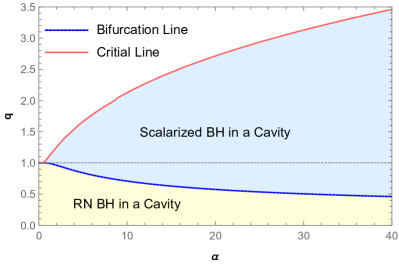
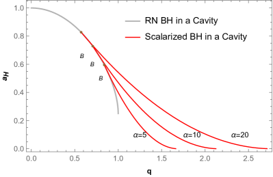
Figure 1: Domain of existence and thermodynamic preference for scalarized RN BH in a cavity. Left panel: Domain of existence in the ${\footnotesize\alpha-q}$ plane, which is displayed by a shaded light blue region and bounded by the bifurcation and critical lines. The blue dashed line represents the bifurcation line, where scalarized black holes bifurcate from RN black holes in a cavity as zero modes. The red line marks critical configurations of scalarized black holes, where the horizon area vanishes with the mass remaining finite. The horizontal dashed gray line denotes extremal RN black holes in cavity, above which RN black hole solutions in a cavity do not exist. Right panel: Reduced area ${\footnotesize a}_{{\footnotesize H}}$ versus reduced charge ${\footnotesize q}$ for RN black holes (a gray line) and scalarized RN black holes with various values of ${\footnotesize q}$ (red lines). For a given ${\footnotesize q}$, ${\footnotesize a}_{{\footnotesize H}}$ of the scalarized RN black hole in a cavity is larger than that of the RN black hole, and increases with the growth of ${\footnotesize\alpha}$. The scalarized black hole solutions are always entropically preferred.

We present the numerical results, e.g., domains of existence, thermodynamic preference and effective potentials, for scalarized black hole solutions in a cavity. We express non-linear differential equation $\left(\ref{eq:EoM}\right)$ in terms of a new coordinate

$$x=1-\frac{r_{+}}{r}\text{ with }0\leq x<1-\frac{r_{+}}{r_{B}},$$ (16)

and employ the NDSolve function in Wolfram Mathematic to numerically solve the equations in the interval $10^{-8}<x<1-r_{+}/r_{B}$. In what follows, we confine ourselves to the simplest case of nodeless, spherically symmetric black hole solutions and leave general configurations for future work.

Figure 2: Effective potentials for scalarized RN black holes with ${\footnotesize\alpha=5}$ for various values of ${\footnotesize q}$. They are all positive definite, which means that the scalarized solutions are stable against radial perturbations.

In the left panel of FIG. $\left(\ref{fig: Criticalline}\right)$, we present the domain of existence for scalarized RN black holes in a cavity with $r_{B}/Q=10$. For a given $\alpha$, scalarized solutions emerge from the bifurcation line as zero modes, and can be continuously induced by increasing $q$ until they reach the critical line. The numerical results suggest that, for scalarized solutions on the critical line, the horizon radius $r_{+}$ vanishes, whereas the mass $M$ and the charge $Q$ remain finite. The domain of existence for scalarized solutions is bounded by the bifurcation and critical lines, and the boundary contour of domain of existence shows a close resemblance to that of RN black holes Herdeiro:2018wub and RN-AdS black holes Guo:2021zed . The numerical results show that there exists a unique set of nodeless scalarized solutions for given $\alpha$ and $q$ in the domain of existence. We plot the reduced area $a_{H}$ of the scalarized solutions against the reduced charge $q$ for several $\alpha$ values of in the right panel of FIG. $\left(\ref{fig: Criticalline}\right)$, which indicates that scalarized solutions are entropically preferred over RN black hole solutions in a cavity.

Then we consider spherically symmetric and time-dependent linear perturbations around the black hole. The metric ansatz including the perturbations can be written as Fernandes:2019rez

$$ds^{2}=-\tilde{N}\left(r,t\right)e^{\tilde{\delta}\left(r,t\right)}dt^{2}+\frac{dr^{2}}{\tilde{N}\left(r,t\right)}+r^{2}\left(d\theta^{2}+\sin^{2}\theta d\varphi^{2}\right),$$ (17)

where

$$\tilde{N}\left(r,t\right)=N\left(r\right)+\epsilon\tilde{N}_{1}\left(r\right)e^{-i\Omega t}\text{ and }\tilde{\delta}\left(r,t\right)=\delta\left(r\right)+\epsilon\tilde{\delta}_{1}\left(r\right)e^{-i\Omega t}.$$ (18)

The time dependence of the perturbations is assumed to be Fourier modes with frequency. Similarly, the ansatzes of the scalar and electromagnetic fields are given by

$$\tilde{\phi}\left(r,t\right)=\phi\left(r\right)+\epsilon\tilde{\phi}_{1}\left(r\right)e^{-i\Omega t}\text{ and }\tilde{V}\left(r,t\right)=V\left(r\right)+\epsilon\tilde{V}_{1}\left(r\right)e^{-i\Omega t},$$ (19)

respectively. Solving eqn. $\left(\ref{eq:IEOM}\right)$ with the ansatzes $\left(\ref{eq:mNp}\right)$ and $\left(\ref{eq:mVp}\right)$, one can extract a Schrodinger-like equation for the perturbative scalar field $\tilde{\phi}_{1}\left(r\right)$,

$$-\frac{d^{2}\Psi\left(r\right)}{dr^{\ast 2}}+U_{\Omega}\Psi\left(r\right)=\Omega^{2}\Psi\left(r\right),$$ (20)

where $\Psi\left(r\right)\equiv r\phi_{1}\left(r\right)$, and the tortoise coordinates $r^{\ast}$ is defined by $dr^{\ast}/dr=e^{\delta\left(r\right)}N^{-1}\left(r\right)$. The effective potential $U_{\Omega}$ is given by

$$U_{\Omega}=\frac{e^{-2\delta}N}{r^{2}}\left[1-N-2r^{2}\phi^{\prime 2}-\frac{Q^{2}}{r^{2}f\left(\phi\right)}\left(1-2r^{2}\phi^{\prime 2}+\frac{\ddot{f}\left(\phi\right)}{2f\left(\phi\right)}+2r\phi^{\prime}\frac{\dot{f}\left(\phi\right)}{f\left(\phi\right)}-\frac{\dot{f}^{2}\left(\phi\right)}{f^{2}\left(\phi\right)}\right)\right],$$

which can be shown to vanish at the event horizon and spatial infinity. A positive definite $U_{\Omega}$ ensures that scalarized black hole solutions are stable against the spherically symmetric perturbations. We display effective potentials for scalarized solutions with $\alpha=5$ in FIG. $\left(\ref{fig:effUvarq}\right)$. The numerics show that the scalarized solutions always have positive effective potentials, thus are stable against the spherically symmetric perturbations.

IV Phase structure

In this section, we consider phase structure and transitions of scalarized and RN black holes in a cavity. For black holes in a cavity, in a canonical ensemble, the wall of the cavity, which is located at $r=r_{B}$, is maintained at a temperature of $T$ and a charge of $Q$. It was showed Braden:1990hw that the system temperature $T$ and charge $Q$ can be related to the black hole temperature $T_{b}$ and charge $Q_{b}$ as

$$Q=Q_{b}\text{ and }T=\frac{T_{b}}{\sqrt{N\left(r_{B}\right)}},$$ (21)

respectively. The Helmholtz free energy $F$ and the thermal energy $E$ were also given in Carlip:2003ne ,

$$F=r_{B}\sqrt{1-N\left(r_{B}\right)}-T\pi r_{+}^{2},\text{ }E=r_{B}\sqrt{1-N\left(r_{B}\right)}.$$ (22)

The phase that has the lowest possible Helmholtz free energy $F$ is the globally stable phase of a multiphase system. The rich phase structure of black holes comes from solving $T\left(r_{+}\right)$ for $r_{+}$. If $T\left(r_{+}\right)$ is a monotonic function with respect to $r_{+}$, there is only one branch for the black hole. More often, there exists a local minimum/maximum for $T\left(r_{+}\right)$ at $r_{+}=r_{+,\min}/r_{+,\max}$. In this case, there is more than one branch for the black hole, corresponding to different phases. The scalar-free RN black holes in a cavity has been studied in Lundgren:2006kt in a canonical ensemble, it show that the thermodynamics and phase structure of RN Black Holes in a cavity is similar to that of AdS counterparts and the critical values is

$$\tilde{r}_{+c}=5-2\sqrt{5},Q_{c}=\sqrt{5}-2,\tilde{T}_{c}=\frac{\sqrt{5+2\sqrt{5}}\left(9-4\sqrt{5}\right)}{2\left(5-2\sqrt{5}\right)^{3}\pi}.$$ (23)

Considering the scalarized black hole solution, there is additional branch for $T\left(r_{+}\right)$. Therefore we displays $\tilde{r}_{+}$ and $\tilde{F}$ against $\tilde{T}$ for scalarized and scalar-free RN black holes in a cavity with different values of $\tilde{Q}$ and $\alpha=5$ in FIG. $\left(\ref{fig:rFTfixQ}\right)$, where

$$\tilde{r}_{+}=\frac{r_{+}}{r_{B}},\text{ }\tilde{F}=\frac{F}{r_{B}},\text{ }\tilde{T}=r_{B}T.$$ (24)

Moreover, the thermodynamic stabilities against thermal fluctuations of these phase is also shown in FIG. $\left(\ref{fig:rFTfixQ}\right)$, where thermodynamic unstable and stable phase is plotted with dashed and solid line, respectively. In a canonical ensemble, the quantity we consider is the specific heat at constant electric charge:

$$C_{Q}=T\left(\frac{\partial S}{\partial T}\right)_{Q}=2\pi r_{+}T\left(\frac{\partial r_{+}}{\partial T}\right)_{Q}.$$ (25)

Since the entropy is proportional to the size of the black hole, a positive specific heat means that the black hole radiates less when it is smaller. Thus, the thermal stability of the branch follows from $C_{Q}>0$.

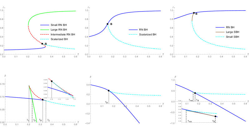
Figure 3: Plots of the reduced horizon radius ${\footnotesize\tilde{r}}_{+}$ and the reduced free energy ${\footnotesize\tilde{F}}$ against the reduced temperature ${\footnotesize\tilde{T}}$ for RN black holes and scalarized black holes in a cavity with different values of ${\footnotesize\tilde{Q}}$ and ${\footnotesize\alpha=5}$. The top row displays ${\footnotesize\tilde{r}}_{+}-{\footnotesize\tilde{T}}$ for various ${\footnotesize\tilde{Q}}$, and the corresponding ${\footnotesize\tilde{F}}-{\footnotesize\tilde{T}}$ is shown in the bottom row. Moreover, the phases plotted by dashed line are thermodynamic unstable since their heat capacity is negative. And black points ${\footnotesize B}$ are bifurcation points. Left Column: ${\footnotesize\tilde{Q}=0.1}$. three scalar-free phases, namely Small RN BH, Intermediate RN BH and Large RN BH, coexist for ${\footnotesize\tilde{T}}_{1}{\footnotesize<\tilde{T}<\tilde{T}}_{2}$ since ${\footnotesize\tilde{Q}<\tilde{Q}}_{c}$. And the scalarized BH exist when ${\footnotesize\tilde{T}>\tilde{T}}_{B}$, where ${\footnotesize\tilde{T}}_{B}$ is the temperature of bifurcation point. And the Small RN BH and Large RN BH are thermodynamic stable, whereas the Intermediate RN BH and Scalarized BH are thermodynamic unstable. Therefore, there is only a first-order phase transition form Small RN BH to Large RN BH at ${\footnotesize\tilde{T}=\tilde{T}}_{p}$. Center Column: ${\footnotesize\tilde{Q}=0.4}$. There are one branch of scalar-free solutions and one branch of scalarized solutions, dubbed RN BH and Scalarized BH. Since the Scalarized BH is thermodynamic unstable, there is no phase transition in this case. Right Column: ${\footnotesize\tilde{Q}=0.8}$. There are one branch of scalar-free solutions and two branch of scalarized solutions, dubbed RN BH, Small Scalarized BH (Small SBH) and Large Scalarized BH (Large SBH). Note that the Large SBH is thermodynamic stable. As ${\footnotesize\tilde{T}}$ increases from ${\footnotesize 0}$, the black hole jumps from the RN BH branch to the Large SBH one, corresponding to the zeroth order phase. Further increasing ${\footnotesize\tilde{T}}$, there would be a first order phase transition returning to the RN BH. Therefore there is a RN BH${\footnotesize\rightarrow}$Large SBH${\footnotesize\rightarrow}$RN BH reentrant phase transition.

When $\tilde{Q}<\tilde{Q}_{c}$, three phases of the scalar-free RN black holes, namely Small BH, Intermediate BH and Large BH, coexist for some range of $\tilde{T}$. And there is only one phase of scalarized RN black holes, which bifurcates form the scalar-free solution. For $\tilde{Q}=0.1<\tilde{Q}_{c}$, we plot $\tilde{r}_{+}$ and $\tilde{F}$ against $\tilde{T}$ in the left column of FIG. $\left(\ref{fig:rFTfixQ}\right)$, where different colored lines represent different phases. The three phases of scalar-free black holes form the characteristic swallowtail, which usually means a van der Waals-like phase transitions. And the scalarized BH bifurcates form Intermediate BH. Moreover, the free energy of scalarized BH is always not the lowest, and the negative specific heat of scalarized BH means that it is thermodynamic unstable. So the scalarized BH is always not globally stable and there is only a first-order transition form Small BH to Large BH at $\tilde{T}=\tilde{T}_{p}$ for $\tilde{Q}<\tilde{Q}_{c}$.

When $\tilde{Q}_{c}<\tilde{Q}<0.49$, there are one branch of scalar-free solutions and one branch of scalarized solutions. The scalar-free one is thermodynamic stable and the scalarized one is thermodynamic unstable. Therefore, the globally stable phase is always scalar-free RN BH, and there is no phase transition, which is shown in the middle column of FIG. $\left(\ref{fig:rFTfixQ}\right)$.

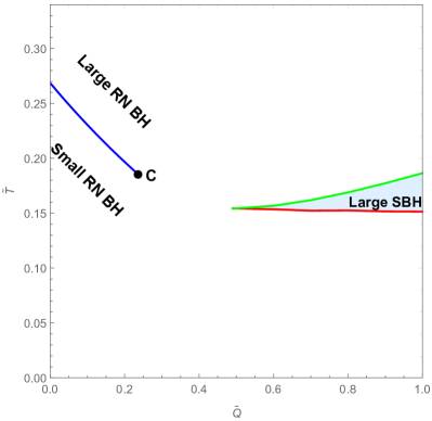
Figure 4: Phase diagrams of RN black holes and scalarized black holes enclosed by a cavity in the $\tilde{Q}$-$\tilde{T}$ plane with ${\small\alpha=10}$. The phase diagram exhibits the globally stable phases, which have the lowest free energy. The first-order phase transition line separating Large BH and Small BH is displayed by blue lines and terminate at the critical point, marked by black dots $C$. In the blue region, the Large scalarized BH (Large SBH) is globally stable. It shown that a reentrant phase transition happens when $\tilde{Q}$ is large enough. This reentrant phase transition consists of a zero-order phase transition and a second-order phase transition, corresponding the red line and green line, respectively.

When $\tilde{Q}>0.49$, there are branches of scalarized black holes, namely Small SBH and Large SBH, coexisting between $\tilde{T}=\tilde{T}_{\min}$ and $\tilde{T}=\tilde{T}_{B}$. The Large SBH has positive specific heat and is thermodynamic stable, whereas the Small SBH is thermodynamic unstable. As $\tilde{T}$ increase from $0$, there is a jumps from the scalar-free RN BH branch to the Large SBH one, corresponding to the zeroth order phase transition between RN BH and Small SBH, followed by a second-order phase transition returning to RN BH. This RN BH$\rightarrow$Large SBH$\rightarrow$RN BH phase transition corresponds to a reentrant phase transition.

Furthermore, we display the globally stable phase of black holes in a cavity in the $\tilde{Q}-\tilde{T}$ plane. In FIG. $\left(\ref{fig:PhaseTQ}\right)$, the blue line represents Large BH/Small BH first-order transition lines, which terminates at the critical point, where a second-order phase transition occurs. The red line and green line correspond the zeroth order phase transition from RN BH to Small SBH and the first order phase transition returning to RN BH, respectively. Comparing with the phase diagram of scalar-free RN black hole in a cavity, the join of scalarized BH results in a additional structure for large enough $\tilde{Q}$, corresponding a reentrant phase transition, which consists of the red line and green line.

V Discussion and Conclusion

In this paper, we investigated spontaneous scalarization of charged black holes enclosed by a cavity in the EMS model with the nonminimal coupling function $f\left(\phi\right)=e^{\alpha\phi^{2}}$, and studied the phase structure of these black holes in a canonical ensemble. The scalarized black holes in a cavity can bifurcate from scalar-free solution on the bifurcation line, which consists of zero modes of the scalar-free solutions. The domains of existence, thermodynamic preference, radial stability and temperature of these solutions were numerically investigated for the black holes in a cavity. In the $\alpha-q$, FIG. $\left(\ref{fig: Criticalline}\right)$ shows that the domain of existence for scalarized RN black holes in a cavity is bounded by the bifurcation and critical lines, which is very similar with the case of not in a cavity Herdeiro:2018wub and RN-AdS Guo:2021zed . Note that the scalarized solutions in a cavity always have positive effective potentials, which means they are always stable against the spherically symmetric perturbations, unlike the case of RN-AdS black holes.

Furthermore, we studied the thermodynamic of these black holes and a richer phase structure than the scalar-free case is displays in FIG. $\left(\ref{fig:PhaseTQ}\right)$. In the small $\tilde{Q}$ regime, scalarized black holes never globally minimize the free energy, there is a classical first-order phase transition line separating Large BH and Small BH, resembling that of the liquid/gas system closely. However, when $\tilde{Q}$ is large enough, there is another structure since scalarized black holes can be the globally stable phase in the large $\tilde{Q}$ regime, where the system undergoes a RN BH$\rightarrow$Large SBH$\rightarrow$RN BH reentrant phase transition as $\tilde{T}$ increases from $0$. And this reentrant phase transition consists of a zeroth-order phase transition and a second-order one.

In this paper, the spontaneous scalarization of black holes in a cavity were studied, and the phase structure is investigated in the normal phase space, where the cavity radius is fixed. The results closely resemble those of the AdS counterparts for scalarized RN black holes. Recently, the phase space of black holes in a cavity has been extended by including a thermodynamic pressure and a thermodynamic volume Wang:2020hjw , it is interesting to consider scalarized black holes enclosed by a cavity in the extended phase space. Moreover, one can study excited scalarized solutions since only the fundamental state was considered in this paper. On the other hand, other thermodynamic properties could be investigated for scalarized black holes in a cavity and it would be very interesting to explore these phenomena in the context of other non-linear electrodynamics black holes in a cavity and check whether analogies with the AdS counterparts can go beyond RN black holes.

- (1) M.S. Volkov and D.V. Galtsov. NonAbelian Einstein Yang-Mills black holes. JETP Lett., 50:346–350, 1989.
- (2) P. Bizon. Colored black holes. Phys. Rev. Lett., 64:2844–2847, 1990. doi:10.1103/PhysRevLett.64.2844.
- (3) Hugh Luckock and Ian Moss. BLACK HOLES HAVE SKYRMION HAIR. Phys. Lett. B, 176:341–345, 1986. doi:10.1016/0370-2693(86)90175-9.
- (4) Serge Droz, Markus Heusler, and Norbert Straumann. New black hole solutions with hair. Phys. Lett. B, 268:371–376, 1991. doi:10.1016/0370-2693(91)91592-J.
- (5) P. Kanti, N.E. Mavromatos, J. Rizos, K. Tamvakis, and E. Winstanley. Dilatonic black holes in higher curvature string gravity. Phys. Rev. D, 54:5049–5058, 1996. arXiv:hep-th/9511071, doi:10.1103/PhysRevD.54.5049.
- (6) Carlos A.R. Herdeiro and Eugen Radu. Asymptotically flat black holes with scalar hair: a review. Int. J. Mod. Phys. D, 24(09):1542014, 2015. arXiv:1504.08209, doi:10.1142/S0218271815420146.
- (7) Thibault Damour and Gilles Esposito-Farese. Nonperturbative strong field effects in tensor - scalar theories of gravitation. Phys. Rev. Lett., 70:2220–2223, 1993. doi:10.1103/PhysRevLett.70.2220.
- (8) Vitor Cardoso, Isabella P. Carucci, Paolo Pani, and Thomas P. Sotiriou. Matter around Kerr black holes in scalar-tensor theories: scalarization and superradiant instability. Phys. Rev. D, 88:044056, 2013. arXiv:1305.6936, doi:10.1103/PhysRevD.88.044056.
- (9) Vitor Cardoso, Isabella P. Carucci, Paolo Pani, and Thomas P. Sotiriou. Black holes with surrounding matter in scalar-tensor theories. Phys. Rev. Lett., 111:111101, 2013. arXiv:1308.6587, doi:10.1103/PhysRevLett.111.111101.
- (10) Daniela D. Doneva and Stoytcho S. Yazadjiev. New Gauss-Bonnet Black Holes with Curvature-Induced Scalarization in Extended Scalar-Tensor Theories. Phys. Rev. Lett., 120(13):131103, 2018. arXiv:1711.01187, doi:10.1103/PhysRevLett.120.131103.
- (11) Hector O. Silva, Jeremy Sakstein, Leonardo Gualtieri, Thomas P. Sotiriou, and Emanuele Berti. Spontaneous scalarization of black holes and compact stars from a Gauss-Bonnet coupling. Phys. Rev. Lett., 120(13):131104, 2018. arXiv:1711.02080, doi:10.1103/PhysRevLett.120.131104.
- (12) G. Antoniou, A. Bakopoulos, and P. Kanti. Evasion of No-Hair Theorems and Novel Black-Hole Solutions in Gauss-Bonnet Theories. Phys. Rev. Lett., 120(13):131102, 2018. arXiv:1711.03390, doi:10.1103/PhysRevLett.120.131102.
- (13) Daniela D. Doneva, Stella Kiorpelidi, Petya G. Nedkova, Eleftherios Papantonopoulos, and Stoytcho S. Yazadjiev. Charged Gauss-Bonnet black holes with curvature induced scalarization in the extended scalar-tensor theories. Phys. Rev. D, 98(10):104056, 2018. arXiv:1809.00844, doi:10.1103/PhysRevD.98.104056.
- (14) Pedro V.P. Cunha, Carlos A.R. Herdeiro, and Eugen Radu. Spontaneously Scalarized Kerr Black Holes in Extended Scalar-Tensor–Gauss-Bonnet Gravity. Phys. Rev. Lett., 123(1):011101, 2019. arXiv:1904.09997, doi:10.1103/PhysRevLett.123.011101.
- (15) Carlos A. R. Herdeiro, Eugen Radu, Hector O. Silva, Thomas P. Sotiriou, and Nicolás Yunes. Spin-induced scalarized black holes. Phys. Rev. Lett., 126(1):011103, 2021. arXiv:2009.03904, doi:10.1103/PhysRevLett.126.011103.
- (16) Carlos A.R. Herdeiro, Eugen Radu, Nicolas Sanchis-Gual, and José A. Font. Spontaneous Scalarization of Charged Black Holes. Phys. Rev. Lett., 121(10):101102, 2018. arXiv:1806.05190, doi:10.1103/PhysRevLett.121.101102.
- (17) Shahar Hod. Analytic treatment of near-extremal charged black holes supporting non-minimally coupled massless scalar clouds. Eur. Phys. J. C, 80(12):1150, 2020. doi:10.1140/epjc/s10052-020-08723-z.
- (18) Pedro G. S. Fernandes, Carlos A. R. Herdeiro, Alexandre M. Pombo, Eugen Radu, and Nicolas Sanchis-Gual. Spontaneous Scalarisation of Charged Black Holes: Coupling Dependence and Dynamical Features. Class. Quant. Grav., 36(13):134002, 2019. [Erratum: Class.Quant.Grav. 37, 049501 (2020)]. arXiv:1902.05079, doi:10.1088/1361-6382/ab23a1.
- (19) Jose Luis Blázquez-Salcedo, Carlos A.R. Herdeiro, Jutta Kunz, Alexandre M. Pombo, and Eugen Radu. Einstein-Maxwell-scalar black holes: the hot, the cold and the bald. Phys. Lett. B, 806:135493, 2020. arXiv:2002.00963, doi:10.1016/j.physletb.2020.135493.
- (20) D. Astefanesei, C. Herdeiro, A. Pombo, and E. Radu. Einstein-Maxwell-scalar black holes: classes of solutions, dyons and extremality. JHEP, 10:078, 2019. arXiv:1905.08304, doi:10.1007/JHEP10(2019)078.
- (21) Pedro G.S. Fernandes, Carlos A.R. Herdeiro, Alexandre M. Pombo, Eugen Radu, and Nicolas Sanchis-Gual. Charged black holes with axionic-type couplings: Classes of solutions and dynamical scalarization. Phys. Rev. D, 100(8):084045, 2019. arXiv:1908.00037, doi:10.1103/PhysRevD.100.084045.
- (22) De-Cheng Zou and Yun Soo Myung. Scalarized charged black holes with scalar mass term. Phys. Rev. D, 100(12):124055, 2019. arXiv:1909.11859, doi:10.1103/PhysRevD.100.124055.
- (23) Pedro G.S. Fernandes. Einstein-Maxwell-scalar black holes with massive and self-interacting scalar hair. Phys. Dark Univ., 30:100716, 2020. arXiv:2003.01045, doi:10.1016/j.dark.2020.100716.
- (24) Yan Peng. Scalarization of horizonless reflecting stars: neutral scalar fields non-minimally coupled to Maxwell fields. Phys. Lett. B, 804:135372, 2020. arXiv:1912.11989, doi:10.1016/j.physletb.2020.135372.
- (25) Yun Soo Myung and De-Cheng Zou. Instability of Reissner–Nordström black hole in Einstein-Maxwell-scalar theory. Eur. Phys. J. C, 79(3):273, 2019. arXiv:1808.02609, doi:10.1140/epjc/s10052-019-6792-6.
- (26) Yun Soo Myung and De-Cheng Zou. Stability of scalarized charged black holes in the Einstein–Maxwell–Scalar theory. Eur. Phys. J. C, 79(8):641, 2019. arXiv:1904.09864, doi:10.1140/epjc/s10052-019-7176-7.
- (27) De-Cheng Zou and Yun Soo Myung. Radial perturbations of the scalarized black holes in Einstein-Maxwell-conformally coupled scalar theory. Phys. Rev. D, 102(6):064011, 2020. arXiv:2005.06677, doi:10.1103/PhysRevD.102.064011.
- (28) Dumitru Astefanesei, Carlos Herdeiro, João Oliveira, and Eugen Radu. Higher dimensional black hole scalarization. JHEP, 09:186, 2020. arXiv:2007.04153, doi:10.1007/JHEP09(2020)186.
- (29) Yun Soo Myung and De-Cheng Zou. Quasinormal modes of scalarized black holes in the Einstein–Maxwell–Scalar theory. Phys. Lett. B, 790:400–407, 2019. arXiv:1812.03604, doi:10.1016/j.physletb.2019.01.046.
- (30) Jose Luis Blázquez-Salcedo, Carlos A.R. Herdeiro, Sarah Kahlen, Jutta Kunz, Alexandre M. Pombo, and Eugen Radu. Quasinormal modes of hot, cold and bald Einstein-Maxwell-scalar black holes. 8 2020. arXiv:2008.11744.
- (31) Yun Soo Myung and De-Cheng Zou. Scalarized charged black holes in the Einstein-Maxwell-Scalar theory with two U(1) fields. Phys. Lett. B, 811:135905, 2020. arXiv:2009.05193, doi:10.1016/j.physletb.2020.135905.
- (32) Yun Soo Myung and De-Cheng Zou. Scalarized black holes in the Einstein-Maxwell-scalar theory with a quasitopological term. Phys. Rev. D, 103(2):024010, 2021. arXiv:2011.09665, doi:10.1103/PhysRevD.103.024010.
- (33) Yves Brihaye, Carlos Herdeiro, and Eugen Radu. Black Hole Spontaneous Scalarisation with a Positive Cosmological Constant. Phys. Lett. B, 802:135269, 2020. arXiv:1910.05286, doi:10.1016/j.physletb.2020.135269.
- (34) Guangzhou Guo, Peng Wang, Houwen Wu, and Haitang Yang. Scalarized Einstein-Maxwell-scalar Black Holes in Anti-de Sitter Spacetime. 2 2021. arXiv:2102.04015.
- (35) Peng Wang, Houwen Wu, and Haitang Yang. Scalarized Einstein-Born-Infeld-scalar Black Holes. 12 2020. arXiv:2012.01066.
- (36) R. A. Konoplya and A. Zhidenko. Analytical representation for metrics of scalarized Einstein-Maxwell black holes and their shadows. Phys. Rev. D, 100(4):044015, 2019. arXiv:1907.05551, doi:10.1103/PhysRevD.100.044015.
- (37) Shahar Hod. Spontaneous scalarization of charged Reissner-Nordstr\”om black holes: Analytic treatment along the existence line. Phys. Lett. B, 798:135025, 2019. arXiv:2002.01948.
- (38) Shahar Hod. Reissner-Nordström black holes supporting nonminimally coupled massive scalar field configurations. Phys. Rev. D, 101(10):104025, 2020. arXiv:2005.10268, doi:10.1103/PhysRevD.101.104025.
- (39) S.W. Hawking. Gravitational radiation from colliding black holes. Phys. Rev. Lett., 26:1344–1346, 1971. doi:10.1103/PhysRevLett.26.1344.
- (40) S.W. Hawking. Black hole explosions. Nature, 248:30–31, 1974. doi:10.1038/248030a0.
- (41) S. W. Hawking. Particle Creation by Black Holes. Commun. Math. Phys., 43:199–220, 1975. [Erratum: Commun.Math.Phys. 46, 206 (1976)]. doi:10.1007/BF02345020.
- (42) James M. Bardeen, B. Carter, and S.W. Hawking. The Four laws of black hole mechanics. Commun. Math. Phys., 31:161–170, 1973. doi:10.1007/BF01645742.
- (43) S.W. Hawking and Don N. Page. Thermodynamics of Black Holes in anti-De Sitter Space. Commun. Math. Phys., 87:577, 1983. doi:10.1007/BF01208266.
- (44) Edward Witten. Anti-de Sitter space, thermal phase transition, and confinement in gauge theories. Adv. Theor. Math. Phys., 2:505–532, 1998. arXiv:hep-th/9803131, doi:10.4310/ATMP.1998.v2.n3.a3.
- (45) Mirjam Cvetic and Steven S. Gubser. Phases of R charged black holes, spinning branes and strongly coupled gauge theories. JHEP, 04:024, 1999. arXiv:hep-th/9902195, doi:10.1088/1126-6708/1999/04/024.
- (46) Andrew Chamblin, Roberto Emparan, Clifford V. Johnson, and Robert C. Myers. Charged AdS black holes and catastrophic holography. Phys. Rev. D, 60:064018, Aug 1999. URL: https://link.aps.org/doi/10.1103/PhysRevD.60.064018, arXiv:hep-th/9902170, doi:10.1103/PhysRevD.60.064018.
- (47) Andrew Chamblin, Roberto Emparan, Clifford V. Johnson, and Robert C. Myers. Holography, thermodynamics and fluctuations of charged AdS black holes. Phys. Rev. D, 60:104026, Oct 1999. URL: https://link.aps.org/doi/10.1103/PhysRevD.60.104026, arXiv:hep-th/9904197, doi:10.1103/PhysRevD.60.104026.
- (48) Marco M. Caldarelli, Guido Cognola, and Dietmar Klemm. Thermodynamics of Kerr-Newman-AdS black holes and conformal field theories. Class. Quant. Grav., 17:399–420, 2000. arXiv:hep-th/9908022, doi:10.1088/0264-9381/17/2/310.
- (49) Rong-Gen Cai. Gauss-Bonnet black holes in AdS spaces. Phys. Rev. D, 65:084014, 2002. arXiv:hep-th/0109133, doi:10.1103/PhysRevD.65.084014.
- (50) Mirjam Cvetic, Shin’ichi Nojiri, and Sergei D. Odintsov. Black hole thermodynamics and negative entropy in de Sitter and anti-de Sitter Einstein-Gauss-Bonnet gravity. Nucl. Phys. B, 628:295–330, 2002. arXiv:hep-th/0112045, doi:10.1016/S0550-3213(02)00075-5.
- (51) Shin’ichi Nojiri and Sergei D. Odintsov. Anti-de Sitter black hole thermodynamics in higher derivative gravity and new confining deconfining phases in dual CFT. Phys. Lett. B, 521:87–95, 2001. [Erratum: Phys.Lett.B 542, 301 (2002)]. arXiv:hep-th/0109122, doi:10.1016/S0370-2693(01)01186-8.
- (52) Jr. York, James W. Black hole thermodynamics and the Euclidean Einstein action. Phys. Rev. D, 33:2092–2099, Apr 1986. URL: https://link.aps.org/doi/10.1103/PhysRevD.33.2092, doi:10.1103/PhysRevD.33.2092.
- (53) Harry W. Braden, J. David Brown, Bernard F. Whiting, and James W. York. Charged black hole in a grand canonical ensemble. Phys. Rev. D, 42:3376–3385, Nov 1990. URL: https://link.aps.org/doi/10.1103/PhysRevD.42.3376, doi:10.1103/PhysRevD.42.3376.
- (54) Steven Carlip and S. Vaidya. Phase transitions and critical behavior for charged black holes. Class. Quant. Grav., 20:3827–3838, 2003. arXiv:gr-qc/0306054, doi:10.1088/0264-9381/20/16/319.
- (55) Andrew P. Lundgren. Charged black hole in a canonical ensemble. Phys. Rev. D, 77:044014, 2008. arXiv:gr-qc/0612119, doi:10.1103/PhysRevD.77.044014.
- (56) Peng Wang, Houwen Wu, Haitang Yang, and Feiyu Yao. Extended Phase Space Thermodynamics for Black Holes in a Cavity. JHEP, 09:154, 2020. arXiv:2006.14349, doi:10.1007/JHEP09(2020)154.
- (57) Peng Wang, Haitang Yang, and Shuxuan Ying. Thermodynamics and phase transition of a Gauss-Bonnet black hole in a cavity. Phys. Rev. D, 101(6):064045, 2020. arXiv:1909.01275, doi:10.1103/PhysRevD.101.064045.
- (58) Peng Wang, Houwen Wu, and Haitang Yang. Thermodynamics and Phase Transition of a Nonlinear Electrodynamics Black Hole in a Cavity. JHEP, 07:002, 2019. arXiv:1901.06216, doi:10.1007/JHEP07(2019)002.
- (59) Kangkai Liang, Peng Wang, Houwen Wu, and Mingtao Yang. Phase structures and transitions of Born–Infeld black holes in a grand canonical ensemble. Eur. Phys. J. C, 80(3):187, 2020. arXiv:1907.00799, doi:10.1140/epjc/s10052-020-7750-z.
- (60) Peng Wang, Houwen Wu, and Haitang Yang. Thermodynamic Geometry of AdS Black Holes and Black Holes in a Cavity. Eur. Phys. J. C, 80(3):216, 2020. arXiv:1910.07874, doi:10.1140/epjc/s10052-020-7776-2.
- (61) Peng Wang, Houwen Wu, and Shuxuan Ying. Validity of Thermodynamic Laws and Weak Cosmic Censorship for AdS Black Holes and Black Holes in a Cavity. 2 2020. arXiv:2002.12233.
- (62) William H. Press and Saul A. Teukolsky. Floating Orbits, Superradiant Scattering and the Black-hole Bomb. Nature, 238:211–212, 1972. doi:10.1038/238211a0.
- (63) Vitor Cardoso, Oscar J. C. Dias, Jose P. S. Lemos, and Shijun Yoshida. The Black hole bomb and superradiant instabilities. Phys. Rev. D, 70:044039, 2004. [Erratum: Phys.Rev.D 70, 049903 (2004)]. arXiv:hep-th/0404096, doi:10.1103/PhysRevD.70.049903.
- (64) Carlos A. R. Herdeiro, Juan Carlos Degollado, and Helgi Freyr Rúnarsson. Rapid growth of superradiant instabilities for charged black holes in a cavity. Phys. Rev. D, 88:063003, 2013. arXiv:1305.5513, doi:10.1103/PhysRevD.88.063003.
- (65) Shahar Hod. Analytic treatment of the charged black-hole-mirror bomb in the highly explosive regime. Phys. Rev. D, 88(6):064055, 2013. arXiv:1310.6101, doi:10.1103/PhysRevD.88.064055.
- (66) Oscar J.C. Dias and Ramon Masachs. Charged black hole bombs in a Minkowski cavity. Class. Quant. Grav., 35(18):184001, 2018. arXiv:1801.10176, doi:10.1088/1361-6382/aad70b.
- (67) Oscar J.C. Dias and Ramon Masachs. Evading no-hair theorems: hairy black holes in a Minkowski box. Phys. Rev. D, 97(12):124030, 2018. arXiv:1802.01603, doi:10.1103/PhysRevD.97.124030.