Neural Video Compression using GANs for Detail Synthesis and Propagation

Abstract

We present the first neural video compression method based on generative adversarial networks (GANs). Our approach significantly outperforms previous neural and non-neural video compression methods in a user study, setting a new state-of-the-art in visual quality for neural methods. We show that the GAN loss is crucial to obtain this high visual quality. Two components make the GAN loss effective: we i) synthesize detail by conditioning the generator on a latent extracted from the warped previous reconstruction to then ii) propagate this detail with high-quality flow. We find that user studies are required to compare methods, i.e., none of our quantitative metrics were able to predict all studies. We present the network design choices in detail, and ablate them with user studies.

1 Introduction

Figure 1: Comparing our reconstruction to various baselines. On the left, we see crops from neural methods, where we compare to the published MSE-based methods RLVC [47], SSF [1], and DVC [23]. On the right we see the original and the non-neural methods, H.264 [4] and HEVC [17]. We see how high frequency texture is faithfully synthesized in our approach, while staying close to the input, where-as MSE-based methods suffer from blurryness. Best viewed on screen.

Recently, there has been progress in neural video compression, leading to the latest approaches being comparable to or even outperforming the non-learned standard codec HEVC [17] in terms of PSNR [1, 48, 33, 20] or outperforming it in MS-SSIM [11, 33, 20]. However, as we navigate the rate-distortion trade-off towards low bitrates, reconstructions become blurry (for neural approaches) or blocky (for non-neural). This was also observed for images, where there has been interest in instead optimizing the rate-distortion-realism trade-off [8, 42, 40, 39]. In short, the goal is to add a realism constraint, forcing the decoder to make sure that reconstructions are also looking “realistic” (in the sense that they are indistinguishable from real images), while still staying close to the input. To optimize this constraint, previous work [2, 24, 37, 34] added a GAN [12] loss to the rate distortion objective, thereby navigating the triple-tradeoff.

However, targeting realism remains largely unexplored for neural video compression. This is perhaps not surprising, as video compression brings various challenges [49], and GAN training is notoriously hard [12]. To apply rate-distortion-realism theory for video, we need to be able to synthesize detail whenever new content appears, and then we need to propagate this detail to future frames. With this in mind, we carefully design a generative neural video compression approach excelling at synthesizing and then preserving detail.

According to the theory [7, 8], realism cannot be measured in terms of pair-wise distortions such as PSNR and MS-SSIM. In fact, theory predicts that these metrics must get worse as realism increases. Following previous work [2, 24], we thus perform extensive user studies to evaluate our approach, where we ask raters to compare methods and chose which “is closest to the original” (see Sec. 4.2). We find that by trading-off just a little bit in PSNR (${\approx}0.6\text{dB}$, see Sec. 5), we can significantly improve in realism, as measured by the study. This way, our approach manages to synthesize small scale detail while staying close to the original (see Fig. 1). Our main contributions are as follows:

1. We present the first GAN-based neural compression system and set a new state-of-the-art in subjective visual quality measured with user studies, where we significantly outperform previous neural compression systems ([1], [47], [23]), as well as the standard codecs H.264 [4] and HEVC [17]. We show that the GAN loss is crucial for this performance.

2. We show that two components are crucial to make the GAN loss effective: i) We condition the generator on a “free” (in terms of bits) latent obtained by feeding the warped previous reconstruction through the image encoder, and show that this is crucial to synthesize details. ii) To be able to propagate previously synthesized details, we rely on accurate optical flow provided by UFlow [18], and warping with high-quality resampling kernels.

2 Related Work

Neural Video Compression

Wu et al. [46] use frame interpolation for video compression, compressing B-frames by interpolating between other frames. Djelouah et al. [10] also use interpolation, but additionally employ an optical flow predictor for warping frames. This approach of using future frames is commonly referred to as “B-frame coding” for “bidirectional prediction”. Other neural video coding methods rely on only using predictive (P) frames, commonly referred to as the “low-delay” setting, since it is more suitable for streaming applications by not relying on future frames. Lu et al. [23] use previously decoded frames and a pretrained optical flow network. Habibian et al. [15] do not explicitly model motion, and instead rely on a 3D autoregressive entropy model to capture spatial and temporal correlations. Liu et al. [21] build temporal priors via LSTMs, while Liu et al. [22] condition entropy models on previous frames. Rippel et al. [35] support adapting the rate during encoding, and also do not explicitly model motion. Agustsson et al. [1] propose “scale-space flow” to avoid complex residuals by allowing the model to blur as needed via a pyramid of blurred versions of the image. Yang et al. [48] generalize various approaches by learning to adapt the residual scale, and conditioning residual entropy models on flow latents. Li et al. [20] use deep features as context for encoding, decoding and entropy coding. Golinsky et al. [11] recurrently connect decoders with subsequent unrolling steps, while Yang et al. [47] also add recurrent entropy models. Rippel and Anderson et al. [33] explore ways to make neural video compression more practical, with models that cover a range of bitrates and a focus on computational efficientcy, improving encode and decode time.

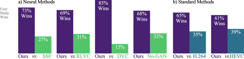
Figure 2: Comparing 6 different pairs of methods in a user study, on MCL-JCV. We visualize how often each method is preferred in the user studies. We had 1639 ratings in total, with an average of 273 per method pair. a) Shows neural methods, SSF [1], RLVC [47], and DVC [23], seeing that our method significantly outperforms them in terms of visual quality. We compare Ours to our no-GAN baseline, where we see that a GAN clearly helps. b) We compare to the standard codecs H.264 [4] and HEVC [17], and see that our method is also preferred.

Non-Neural Video Compression

The combination of transform coding [14] using discrete cosine transforms [3] with spatial and/or temporal prediction, known as “Hybrid video coding”, emerged in the 1980s as the technology dominating video compression until the present day. Non-neural methods such as H.261 through H.265/HEVC [17], VP8 [6], VP9 [29] and AV1 [9] have all remained faithful to the hybrid coding principle, with extensive refinements, regarding more flexible pixel formats (e.g., bit depth, chroma subsampling), more flexible temporal and spatial prediction (e.g., I-, P-, B-frames, intra block copy), and many more. Thanks to the years of research that went into these codecs, they provide strong baselines for neural approaches.

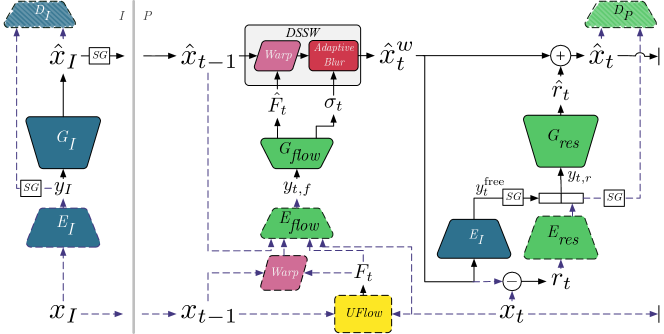
$F_{t}$
$\sigma_{t}$
$r_{t}$

Figure 3: Architecture overview, with some intermediate tensors visualized in the gray box. To the left of the gray line is the I-frame branch (learned CNNs in blue), to the right the P-frame branch (learned CNNs in green). Dashed lines are not active during decoding, and discriminators $D_{I},D_{P}$ are only active during training. The size of the CNN blocks roughly indicates their capacity. SG is a stop gradient operation. DSSW is our “decouped scale-space warping” (Sec. 3.2), and UFlow is a frozen optical flow model from [18].

3 Method

3.1 Overview

An overview of the architecture we use is given in Fig. 3, while a detailed view with all layers is provided in App. Fig. 14. Let $x=\{x_{1},x_{2},\dots\}$ be a sequence of frames, where $x_{1}$ is the initial (I) frame, denoted by $x_{I}$ in the figure and below. Similar to previous work, we operate in the “low-delay” mode, and hence predict subsequent (P) frames from previous frames. Let $\hat{x}=\{\hat{x}_{1},\hat{x}_{2},\dots\}$ be the reconstructed video. We use the following strategy to obtain high-fidelity reconstructions:

1. Synthesize plausible details in the I-frame.

2. Propagate those details wherever possible and as sharp as possible.

3. For new content appearing in P-frames, we again want to synthesize plausible details.

As mentioned in the Introduction, we optimize for perceptual quality and distortion, and note that the above three points are in contrast to purely distortion-optimized neural video codecs, which, particularly at low bitrates, favor blurring detail to reduce the distortion loss. Instead, our approach will be able to synthesize faithful texture, while still staying close to the input, as seen in Fig. 1.

The I-frame branch is based on a lightweight version of the architecture used in “HiFiC” [24] (mostly making it less wide, see App. Fig. 14), and is used to address (S1). In detail, the encoder CNN $E_{I}$ maps the input image $x_{I}$ to a quantized latent $y_{I}$, which is entropy coded using a hyperprior [26] (not shown in Fig. 3, but which is detailed in App. Fig. 14). From the decoded $y_{I}$, we obtain a reconstruction $\hat{x}_{I}$ via the I-generator $G_{I}$. We use an I-frame discriminator $D_{I}$ that—following [24]—is conditioned on the latent $z_{I}$ (we elaborate on conditioning in Sec. 3.5).

The P-frame branch has two parts, an auto-encoder $E_{\textit{flow}}$, $G_{\textit{flow}}$ for the flow, and an auto-encoder $E_{\textit{res}},G_{\textit{res}}$ for the residual, following previous video work (e.g. [23, 1], etc.). To partially address (S2), similar to previous work, we employ a powerful optical flow predictor network on the encoder side, UFlow [18]. The resulting (backward) flow $F_{t}=\textit{UFlow}(x_{t},x_{t-1})$ is fed to the flow-encoder $E_{\textit{flow}}$, which outputs the quantized and entropy-coded flow-latent $y_{t,f}$. From the flow-latent, the generator $G_{\textit{flow}}$ predicts both a reconstructed flow $\hat{F}_{t}$, as well as a mask $\sigma_{t}$. The mask $\sigma_{t}$ has the same spatial dimensions as $F_{t}$, with each value in $[0,\sigma_{\text{max}}]$. Together, $(\hat{F}_{t},\sigma_{t})$ are used for our decoupled scale-space warping, a variant of scale-space warping [1], described in Sec. 3.2. Intuitively, for each pixel, the mask $\sigma_{t}$ predicts how “correct” the flow at that pixel is (see the gray box in Fig. 3). We first warp the previous reconstruction $\hat{x}_{t-1}$ using $\hat{F}_{t}$, then we use $\sigma_{t}$ to decide how much to blur each pixel. In practice, we observe $\sigma_{t}$ predicts where new content that is not well captured by warping appears. Since the flow is in general relatively easy to compress, we employ shallow networks for $E_{\textit{flow}}$ and $G_{\textit{flow}}$ based on networks used in image compression [26]. We denote the resulting warped and potentially blurred previous reconstruction with $\hat{x}_{t}^{w}$.

Finally, we calculate the residual $r_{t}=x_{t}-\hat{x}_{t}^{w}$ and compress it with the residual auto-encoder $E_{\textit{res}},G_{\textit{res}}$. To address the last point above, (S3), we again employ the light version of the HiFiC architecture for $E_{\textit{res}},G_{\textit{res}}$. However, we introduce one important component. We observe that $G_{\textit{res}}$ is not able to synthesize high-frequency details from the sparse residual latent $E_{\textit{res}}(r_{t})$ alone. However, we found that additionally feeding a “free” latent extracted from the warped previous reconstruction $y_{t}^{\text{free}}=E_{I}(\hat{x}_{t}^{w})$ significantly increased the amount of synthesized detail, possibly due to the additional information and context provided by $\hat{x}_{t}^{w}$. Note that this latent does not need to be encoded into the bitstream because the decoder already has $\hat{x}_{t}^{w}$ and can compute $y_{t}^{\text{free}}$ directly (hence it is “free”), and thus also does not need to be quantized. Instead, we concatenate it to $E_{\textit{res}}(r_{t})$ as a source of information, forming $y_{t,r}{=}\text{concat}(y_{t}^{\text{free}},E_{\textit{res}}(r_{t}))$.

To train the P-frame branch, we employ a seperate P-frame discriminator $D_{P}$, with the same architecture as $D_{I}$, conditioned on the generator input $y_{t,r}$.

Bilinear Resampling Kernel    Bicubic Resampling Kernel

Figure 4: To avoid blurry results when repeatedly warping, the quality of the resampling kernel is crucial. Here, we compare shifting an images 20 times with a fixed flow of 0.5px to the left for bilinear and bicubic.

Input $x_{t}$	Output $\hat{x}_{t}$ for different models
	Ours (with GAN	No GAN loss ($\beta{=}0$)	No free latent $y_{t}^{\text{free}}$
	and free latent)

Uncompressed Flow $F_{t}$	Compressed Flow $\hat{F}_{t}$ for different models
	Ours (with UFlow and	Without UFlow	No flow loss ($k_{\text{flow}}{=}0$)
	$k_{\text{flow}}{=}1$)

Figure 5: Visual examples for our ablations, see Sec. 5.1 for details. Top: Our model faithfully reconstructs details of the input, whereas disabling the GAN loss or removing the free latent introduces blurryness like in MSE models. Bottom: Not using supervised optical flow (UFlow) gives poor quality flows. Not using the flow loss makes the flow slightly burrier.

3.2 Decoupled Scale-Space Warping

When warping previously reconstructed frames, we want to preserve detail as much as possible (whether real or synthesized, per (S2) above). Previous neural video compression approaches have commonly used bi-linear warping [23, 10, 35, 47], or tri-linear scale-space warping (SSW) [1, 33, 48]. However it is known from signal processing theory (see e.g. Nehab et al. [30, Fig. 10.6 on p. 64]) that for repeated applications of re-sampling, the quality of the interpolation kernel is crucial to avoid low-pass filtering the signal and blurring out details. We visualize this phenomenon in Fig. 4.

Motivated by these observations, we were interested in implementing the more powerful bicubic warping in SSW, but found that this makes the implementation significantly more complex when combined with the 3-D indexing of scale-space warping. Instead, to be able to efficiently use bicubic warping (and arbitrary other warping operations), we propose a variant of scale-space warping [1], where we decouple the operation into two steps: plain warping, followed by spatially adaptive blurring. We can then use off-the-shelf warping implementations for the first part.

Both variants, at their core, use the scale-space flow field $(\hat{F},\sigma)$, which generalizes optical flow $\hat{F}$ by also specifying a “scale” $\sigma$, such that we get a triplet $(u_{ij},v_{ij},\sigma_{ij})$ for each target pixel $(i,j)$, where $u_{ij},v_{ij}$ are the flow coordinates, and $\sigma_{ij}$ is the blurring scale to use. We recall the method from [1]: To compute a scale-space warped result

$$x_{\text{out}}=\text{SSW}(x,\hat{F},\sigma),$$ (1)

the source $x$ is first repeatedly convolved with Gaussian blur kernels to obtain a “scale-space volume” with $L$ levels,

$$V(x)=[x,x\ast G(s_{1}),\cdots,x\ast G(s_{L-1})],$$ (2)

where $G(s_{i})$ is the Gaussian blur kernel with std. deviation $s_{i}$, and $\{s_{1},\dots,s_{L-1}\}$ are hyperparameters defining how blurry each level in the volume is. The three coordinates of the scale-space flow field $(u_{ij},v_{ij},\sigma_{ij})$ are then used to jointly warp and blur the source image, retrieving pixels via tri-linear interpolation from the scale-space volume.

We obtain a Decoupled SSW (DSSW) result by combining plain warping with spatially adaptive blurring (AB),

$$x_{\text{out}}^{\prime}=\text{DSSW}(x,\hat{F},\sigma)=\text{AB}(\text{Warp}(x,\hat{F}),\sigma),$$ (3)

where Warp is plain warping, and AB is functionally the same as SSW with a zero flow, i.e. $\text{AB}(y,\sigma):=\text{SSW}(y,0,\sigma)$, but can be implemented with a few lines of code using simple multiplicative masks for each level in the scale-space volume to apply the 1-D linear interpolation for each pixel (code in App. 0.A.3).

Together, bicubic warping and adaptive blurring help to propagate sharp detail when needed, while also facilitating smooth blurring when needed (e.g., for focus changes in the video). See App. Fig. 12 for a visualization of how a given input and sigma field $\sigma_{t}$ get blurred via scale-space blur.

We found that on a GPU, DSSW using an optimized warping implementation and our AB was $2{-}3{\times}$ faster than a naive SSW implementation. In App. 0.A.3, we validate our implementation by training models for MSE, and showing that DSSW with bilinear warping obtains similar PSNR as SSW, and DSSW with bicubic warping yields a better model.

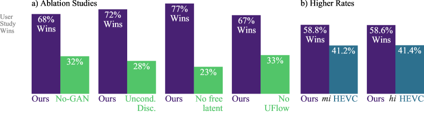
Figure 6: a) User study for Ablations. We see that disabling the GAN loss ($\beta{=}0$), using an unconditional discriminator, or not using the free latent hurts performance. On the flow side, not using UFlow hurts. b) Comparing models at higher rates, targeting $0.14$bpp (mi) and $0.22$bpp (hi).

3.3 Adaptive Proportional Rate Control

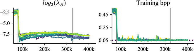
Figure 7: Visualizing the effect of the rate controller for a broad family of models with different hyper parameters, trained for 400k steps. The rate parameter $\lambda_{R}$ is automatically adapted during training (left) to match the target bpp of 0.05 for all models (right). At 80k steps we drop the target rate, at 325k steps we drop the learning rate.

We train our system by optimizing the rate-distortion-perception trade-off [8, 24], and we describe our formulation and loss in Sec. 3.5, but here we want to focus on one hyper-parameter in this trade-off (that also typically appears in the rate-distortion trade-off optimized by previous work): the weight on the bitrate, $\lambda_{R}$. It controls the trade-off between bitrate and other loss terms (distortion, GAN loss, etc.). Unfortunately, since there is no direct relationship between $\lambda_{R}$ and the bitrate of the model when we vary other hyper-parameters, comparison across models is practically impossible, since they end up at different rates if we vary other hyper parameters, in particular other loss weights.

Van Rozendaal et al. [36] also observe this and propose targeting a fixed distortion via constraint optimization. Another approach was used in [24], where $\lambda_{R}$ was dynamically selected from a small $\lambda_{1}$ and a large $\lambda_{2}$, depending on whether the model bitrate was below or above a given target. This approach can be interpreted as an “on-off” controller, but still some requires tuning of $\lambda_{1},\lambda_{2}$.

A natural generalization is to use a proportional-controller: We measure the error between the current mini-batch bitrate $b$ to a target bitrate $b_{t}$ (in log-space), and apply it with a proportional controller to update $\lambda_{R}$ as follows:

$$\log_{2}(\lambda_{R})\leftarrow\log_{2}(\lambda_{R})+k_{P}(\log(b+\epsilon)-\log(b_{t}+\epsilon)),$$ (4)

where $\epsilon=1\textsc{e}{-9}$ for stability and the “proportional gain” $k_{P}$ is a hyperparameter. We note that if we ignore the log-reparameterization, this corresponds to the “Basic Differential Multiplier Method” [32].

This approach is highly effective to obtain models that are comparable in terms of bitrate, despite different hyper-parameters such as learning rates, amount of unrolling, loss weights, etc., as visualized in Fig. 7.

3.4 Sequence Length Train/Test Mismatch

One problem in neural video compression is the train/test mismatch in sequence length: Typically, neural approaches are trained on a handful of frames (e.g., three frames for [1] and five for [21]), and evaluated on hundreds of frames, which can lead to error patterns that emorge during evaluation. While the unrolling behavior is already a problem for MSE-optimized neural codecs (some previous works use small GOPs of 8-12 frames for evaluation to limit temporal error propagation), it requires even more care when detail is synthesized in a generative setting. Since we aim to synthesize high-frequency detail whenever new content appears, incorrectly propagating that detail will create significant visual artifacts. Ideally, we could train with sequences as long as what we evaluate on (i.e., at least $T{=}60$ frames), but in practice this is infeasible on current hardware due to memory and computational constraints. While we can fit up to $T{=}12$ into our accelerators, training then becomes prohibitively slow.

To work towards preventing unrolling issues, as well as accelerating prototyping and training new models, we instead adopt the following scheme: 1) Train $E_{I},G_{I},D_{I}$ only, on randomly selected frames, for $1\,000\,000$ steps. 2) Freeze $E_{I},G_{I},D_{I}$ and initialize the weights of $E_{\textit{res}},G_{\textit{res}}$ from $E_{I},G_{I}$. Train $E_{\textit{flow}}$, $G_{\textit{flow}}$, $E_{\textit{res}}$, $G_{\textit{res}}$, $D_{P}$ for $400\,000$ additional steps using staged unrolling, that is, use $T{=}2$ until $80k$ steps, $T{=}3$ until $300k$, $T{=}4$ until $350k$, and $T{=}6$ until $400k$. This splitting into steps 1) and 2) means trained $E_{I},G_{I}$ can be re-used for many variants of the P-frame branch, and, as a bonus, sharing $E_{I},G_{I}$ across models makes them more comparable. For training times, see App. 0.A.7.

Some error accumulation remains, which we address in two ways: We quantize the frame buffer at each step, i.e., during inference, we always quantize $\hat{x}_{t}$, to be closer to the (8-bit quantized) input. Additionally, we randomly shift reconstructions in each step, to avoid overlapping larger-scale error patterns from accumulating. Together, these techniques help to get rid of most error patterns.

3.5 Formulation and Loss

We base our formulation on HiFiC [24] and optimize the rate-distortion-perception trade-off [8]. We use conditional GANs [12, 28], where both the generator and the discriminator have access to additional labels. As a short recap, the general conditional GAN formulation assumes data points $x$ and labels $s$ following some joint distribution $p(x,s)$. The generator is supposed to map samples $s\sim p(s)$ to the distribution $p(x|s)$, and the discriminator is supposed to predict whether a given pair $(x,s)$ is from the real distribution $p(x|s)$, or from the generator distribution $p(\hat{x}|s)$.

In contrast to HiFiC, we are working with sequences of frames and reconstructions, however, we aim for per-frame distribution matching, i.e., for $T$-length video sequences, the goal is to obtain a model s.t.:

$$p(\hat{x}_{t}|y_{t})=p(x_{t}|y_{t})\quad\forall t\in\{1,\dots,T\},$$ (5)

where $x_{t}$ are inputs, $\hat{x}_{t}$ reconstructions (as above), and we condition both the generators and the discriminators on latents $y_{t}$, using $y_{1}{=}y_{I}$ for the I-frame, $y_{t}{=}y_{t,r}$ for P-frames ($t{>}1$). To readers more familiar with conditional generative video synthesis (e.g., Wang et al. [44]), this simplification may seem sub-optimal as it may lead to temporal consistency issues (i.e., you may imagine that reconstructions $\hat{x}_{t},\hat{x}_{t+1}$ are inconsistent). We emphasize that since we are doing compression, we will also have a per-frame distortion loss (MSE), and we have information that we transmit to the decoder via a bitstream. So while the residual generator can in theory produce arbitrarily inconsistent reconstructions, in practice, these two points appear to be sufficient for preventing any temporal inconsistency issues in our models. We nevertheless explored variations where the discriminator is based on more frames, but this did not significantly alter reconstructions.

Continuing from Eq. 5, we define the overall loss for the I-frame branch and its discriminator $D_{I}$ as follows. We use the “non-saturating” GAN loss [12]. To simplify notation, let $y_{I}=E_{I}(x_{I}),\hat{x}_{I}=G_{I}(y_{I})$:

$$\vspace{-.5em}\mathcal{L}_{\textit{I-Frame}} =\mathbb{E}_{x_{I}\sim p(x_{I})}\bigl{[}\lambda_{R}^{I}r(y_{I})+d(x_{I},\hat{x}_{I})-\beta\log(D_{I}(\hat{x}_{I},y_{I}))\bigr{]},$$ (6)

$$\mathcal{L}_{D_{I}} =\mathbb{E}_{x_{I}\sim p(x_{I})}\bigl{[}-\log(1-D_{I}(\hat{x}_{I},y_{I}))-\log(D_{I}(x_{I},y_{I}))\bigr{]},$$ (7)

where $\lambda_{R}^{I}$ is the adaptive rate controller described in Sec. 3.3, $\beta$ is the GAN loss weight, and $d$ is a per-frame distortion. We use $d{=}\text{MSE}$, i.e., in contrast to HiFiC [24], we do not use a perceptual distortion such as LPIPS. We found no benefit in training with LPIPS, possibly due to a more balanced hyper-parameter selection, and removing it speeds up training by ${\approx}35\%$.

For the P-frame branch, let $p(x_{1}^{T})$ be the distribution of $T$-length clips, where we use $x_{1}$ as the I-frame, and let

$$\mathcal{L}_{\textit{P-Frame}}=\mathbb{E}_{p(x_{1}^{T})} \bigl{[}\textstyle\sum_{t=2}^{T}\lambda_{R}^{P}r(y_{t,r})+td(x_{t},\hat{x}_{t})-t\beta\log(D_{P}(\hat{x}_{t},y_{t,r}))+\mathcal{L}_{\text{reg}}\bigr{]},$$ (8)

$$\mathcal{L}_{D_{P}}=\mathbb{E}_{p(x_{1}^{T})} \bigl{[}\textstyle\sum_{t=2}^{T}-t\log(1-D_{P}(\hat{x}_{t},y_{t,r}))-t\log(D_{P}(x_{I},y_{t,r})))\bigr{]}.$$ (9)

Note that we scale the losses of the $t$-th frame with $t$. This is motivated by the observation that $\hat{x}_{t}$ influences all $T-t$ reconstructions following it, and hence earlier frames indirectly have more influence on the overall loss. Scaling with $t$ ensures all frames have similar influence.

Additionally, we employ a simple regularizer for the P-frame branch:

$$\mathcal{L}_{\text{reg}}=k_{\text{flow}}\cdot\texttt{SG}(\sigma_{t})\cdot L_{2}(F_{t},\hat{F}_{t})+k_{\text{TV}}\textit{TV}(\sigma_{t}),$$ (10)

where the first part is an MSE on the flow, ensuring that $E_{\textit{flow}},G_{\textit{flow}}$ learn to reproduce the flow from UFlow. We mask it with the sigma field, since we only require consistent flow where the network actually uses the flow (but add a stop gradient, SG, to avoid minimizing the loss by just predicting $\sigma_{t}=0$). TV is a total-variation loss [38] ensuring a smooth sigma field.

4 Experiments

4.1 Datasets

Our training data contains $992$k spatio-temporal crops of dimension $256{\times}256$, each containing 12 frames, obtained from videos from YouTube. For training, we randomly choose a contiguous sub-sequence of length $T\in\{2,3,4,5\}$, see Sec. 3.4. The videos are filtered to originally be at least 1080p in resolution, 16:9, 30fps. We omit content labeled as “video games” or “computer generated graphics”, using YouTube’s category system [50]. We evaluate our model on the 30 videos of MCL-JCV [43], which is available under a permissive license from USC, in contrast to, e.g., the HEVC test sequences, which are not publicly available. MCL-JCV contains a broad variety of content types and difficulty, including a wide variety of motion from natural videos, computer animation and classical animation.

4.2 User Study

2AFC

We evaluate our method in a user study, where we ask human raters to rate pairs of methods, i.e., our setup is “two alternatives, forced choice” (2AFC). We implement 2AFC by showing raters two videos side-by-side, where the right video is always the original. On the left, raters see either a video from method A or method B. They can toggle between A and B in-place. We always shuffle the methods, i.e., Ours is not always method A. We use all 30 videos from MCL-JCV, and show the first 2 seconds (to avoid large file sizes, see below), playing in a loop, but raters are allowed to pause videos. Raters are asked to select the video “is closest to the original” (the GUI is shown in the inline figure, exact instructions in App. Fig. 8). This protocol is inspired by previous work in image compression [24, 41], and ensures that differences between methods are easy to spot.

Several considerations went into these choices: For generative video compression, it is important to be able to compare to the original, as otherwise the method may, e.g., completely change colors or content. However, we do not require pixel-perfect reconstructions, which is why we show the original on the right, and not in-place. Methods can be very similar, which is why we allow in-place switching between methods to be able to spot differences.

Rater Qualifications

Our raters are contracted through the “Google Cloud AI Labeling Service” [13]. For each pair of methods, raters are asked to rate all 30 videos of MCL-JCV. In order to make sure our ratings have a high quality, we intersperse five golden questions at random locations into each study, where we compare HEVC at quality factor $Q{=}27$ to $Q{=}35$ ($Q{=}27$ yields bitrates similar to what we study, and $Q{=}35$ is ${\approx}0.023$bpp and contains significant blurring artifacts). We filter out raters who do not correctly answer 4 out of 5 of these questions. Overall, this yields 8-14 raters per study. To ensure that our results are repeatable, we re-do the study after three days.

Shipping Videos to Raters

In order to play back the videos in a web browser we transcode all methods with VP9 [29], using a very high quality factor to avoid any new artifacts. To ensure consistency, and to be sure that the raters can fit the task in their web browser, we center-crop the videos to $1080\times 1080$. This yields large file sizes, so to ensure smooth playback, we focus on the first 2 seconds (60 frames) of each video.

4.3 Metrics and Models

In order to assess how quantitative metrics predict the user study, we employ the well-known PSNR and MSSSIM [45]. We use LPIPS [51] (which measures a distance in AlexNet [19] features space) and PIM (an unsupervised quality metric), as well as FID [16]. Following HiFiC [24] we evaluate FID on non-overlapping $256{\times}256$ patches (see App. A.7 in [24]). Finally, we use VMAF [31], developed by Netflix to evaluate video codecs. We calculate these metrics on the exact sequences we ship to raters.

We refer to our model as Ours, and report all hyper-parameters in App. 0.A.6. To assess the effect of the GAN loss, we train a no-GAN baseline, which uses exactly the same architecture and training schedule as Ours, but is trained without a GAN loss ($\beta{=}0$ in Eqs. (6), (8)). We compare to three neural codecs: SSF, by Agustsson et al. [1], CVPR’2020, RLVC by Yang et al. [47], J-STSP’2021, and DVC by Lu et al. [23], CVPR’2019. For SSF and RLVC, we obtained reconstructions from the authors, for DVC we ran the open-sourced code ourselves and verified that this does match their published numbers on the UVG dataset [25] (exact details in App. 0.A.4). We ran user studies comparing all these models against our proposed GAN model. In contrast to most previous work, we do not constrain our model to use a small GoP size, and instead only use an I-frame for the first frame. For the neural models, we used the GoP from the respective papers ($\infty$ for SSF, 10 for DVC, 12 for RLVC), and we do not constrain the GoP for H.264 and HEVC. The neural codecs we compare to do not densely cover the bitrate axis, so to ensure fair studies, we fix Ours to a model targeting ${\approx}0.07$bpp, and then select a different competing model for each video to match filesizes as closely as possible. The resulting average bpps are at most ${\approx}3\%$ smaller or at most ${\approx}24\%$ bigger than our method. We emphasize that we would have liked to compare to even more neural models, but found no additional code or reconstructions.

Furthermore, we compare against the non-neural standard codecs H.264 and HEVC. We follow best practice and make sure to minimally constrain the codecs, thus using the default “medium” preset (note that some previous works used “fast” or even “veryfast”). Like our method, we run the codecs in the low-latency setting (disabling B-frames). The exact (short) ffmpeg commands are listed in App. 0.A.1. We also run the codecs at ${\approx}0.07$bpp. To get an idea how models compare at higher rates, we fruther run HEVC at ${\approx}0.14$ and ${\approx}0.22$bpp.

On Padding and Bitrates

A problem faced by all CNN-based neural compression codecs is: what happens if the stride of the network does not divide the input resolution. For example, our encoder downscales 4 times, and thus needs the input resolution to divide 16. Like most previous work, we solve this by padding input frames (e.g., $1080{\times}1920$ gets padded to $1088{\times}1920$), obtaining the bitstream of the padded image, obtaining the reconstruction, cropping the reconstruction back to the input resolution, and calculating bpp w.r.t. the input resolution (calculating it w.r.t. the padded resolution would amount to cheating). We note that the RLVC reconstructions were cropped to 1066 pixels, and we thus performed that user study in a cropped setting, and we had to add padding support to the DVC code, which may account for some differences in PSNR (DVC seems to have calculated on cropped images).

	Ours	SSF	Predicts?	RLVC	Predicts?	DVC	Predicts?	No-GAN	Predicts?	H.264	Predicts?	HEVC	Predicts?
PSNR$\uparrow$	34.5	34.8	No≈	34.0	Yes	31.7	Yes	35.1	No	34.6	No≈	35.6	No
MS-SSIM$\uparrow$	0.964	0.963	No≈	0.965	No≈	0.95	Yes	0.967	No≈	0.963	No≈	0.966	No≈
VMAF$\uparrow$	87.3	84.8	Yes	83.1	Yes	81.9	Yes	86.9	No≈	87.7	No≈	91.1	No
PIM-1$\downarrow$	3.34	4.69	Yes	4.93	Yes	6.91	Yes	4.17	Yes	3.17	No	2.62	No
LPIPS$\downarrow$	0.168	0.224	Yes	0.224	Yes	0.26	Yes	0.194	Yes	0.169	No≈	0.147	No
FID/256$\downarrow$	32.8	54.1	Yes	50.3	Yes	61.6	Yes	35.7	Yes	33.0	No≈	24.2	No
Preferred vs. Ours$\uparrow$		27%		31%		15%		32%		35%		39%

Table 1: We show metrics corresponding to the user studies, where the last row repeats the results from Fig. 2. We indicate whether each metric predicts the study, using Yes and No. If the values are within 1% of each other, the metric also does not predict the study, and we indicate this with No_≈. $\uparrow$ indicates that higher is better for this row, $\downarrow$ the opposite. We can see that no metric predicts all user studies (since Ours is preferred in all studies).

5 Results

We show visual results in Fig. 1. We can see how our approach faithfully synthesizes texture and looks very similar to the original, whereas MSE-based approaches suffer from blurryness. The quantitative results from our user study are shown in Fig. 2. At a high level, we see that Ours is preferred by the majority in all studies. Ours vs. no-GAN shows that the GAN loss significantly improves visual quality. The first three studies show that our method significantly outperforms all neural baselines. The standard codecs fare somewhat better, yet our method is clearly preferred overall. We show the comparison at higher rates in Fig. 6b, where the gap between methods gets smaller, but our method is still preferred.

In Table 1 we explore which metrics are able to predict the user study results from Fig. 2. We show values of all methods on all metrics, and indicate whether the metrics predicts the corresponding study. E.g., we can see there that we are preferred over no-GAN in the user study, yet our method has 34.5dB PSNR, while no-GAN has 35.1dB (better), thus PSNR does not predict this study correctly, and we write “No”. Overall, none of the metrics are able to predict all studies. However, we find that the three “perceptual” metrics PIM, LPIPS, and FID/256 all predict the studies of the neural codecs. Unfortunately, none of them predicts the studies involving the standard codecs.

The table also shows how we trade-off distortion (PSNR) for improved realism/visual quality. In the comparison against no-GAN, we can see that 0.6dB in PSNR is traded for being preferred 68% of the time in the user study.

In App. 0.A.2, we show that we were able to obtain the same overall results when running the studies with the same raters three days later, with an even wider gap, and more raters passing the golden study. We also present statistics: how long raters take to answer questions, how often they flip, and how often they pause. We split this data by experiment, by video, and by worker. Averaged over all studies, raters take $26.4$s per comparison, flip $13.5$ times, and pause $0.967$ times. To facilitate further research, we provide links to reconstructions and raw user study data in App. 0.B.

5.1 Ablations

We ablate our main components, using a user study (shown in Fig. 6a) and visually (in Fig. 5). We do ablations by removing parts: In No-GAN, we disable the GAN loss ($\beta=0$), for No free latent we train without the free latent $y_{t}^{\text{free}}$, and in Uncond. Disc., we train with an unconditional discriminator (i.e., $D$ does not see any latents). We can see that all of these perform significantly worse in terms of visual quality (Fig. 6), and lead to blurry reconstruction (Fig. 5, uncond. disc. is not shown but looks similar to No-GAN). In No UFlow, we disable UFlow, i.e., if we do not feed $F_{t}$ to $E_{\textit{flow}}$, and instead let $E_{\textit{flow}}$ learn flow unsupervised from frames, which performs significantly worse (Fig. 6).

6 Conclusion

We presented a GAN-based approach to neural video compression, that significantly outperforms previous neural and non-neural methods, as measured in a user study. With additional user studies, we showed that two components are crucial: i) conditioning the residual generator on a latent obtained from the warped previous reconstruction, and ii) leveraging accurate flow from an optical flow network. Furthermore, we showed how to decouple scale-space warping to be able to leverage high quality resampling kernels, and we used adaptive rate control to ensure consistent bitrates across a wide range of hyperparameters.

Limitations

As we saw, the quantitative metrics we currently have cannot be fully relied on, and hence we have to do user studies. However, this is expensive and not very scalable, and further research into perceptual metrics is needed. We hope that by releasing our reconstructions, we can encourage research in this direction.

Appendix 0.A Appendix

0.A.1 HEVC/H.264 commands

We use ffmpeg, v4.3.2, to encode videos with HEVC and H264. We use the medium preset, and no B-frames, as mentioned in Sec 4.3. We compress each video using quality factors $\texttt{\$Q}\in\{10,\dots,35\}$ to find bpps that match our models, using the following commands:

ffmpeg -i $INPUT_FILE -c:v h264 \
    -crf $Q -preset medium \
    -bf 0 $OUTPUT_FILE

ffmpeg -i $INPUT_FILE -c:v hevc \
    -crf $Q -preset medium \
    -x265-params bframes=0 $OUTPUT_FILE

0.A.2 User Study Details

• Metrics for all ablation studies from Fig. 6 are shown in Table 2

• The result of repeating the user studies three days later is shown in Fig. 8 (top).

• Rater instructions are shown in Fig. 8 (bottom).

• We show user study statistics in Fig. 9, see caption for details.

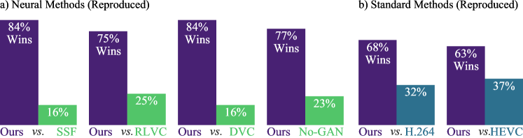
Figure 8: Top: Study repeated 3 days later. Bottom: Instructions shown to the raters.

	Ours	No-GAN	Predicts?	Uncond. Disc.	Predicts?	No free latent	Predicts?	No UFlow	Predicts?	HEVC	Predicts?	HEVC	Predicts?
PSNR$\uparrow$	34.5	35.1	No	34.8	No≈	33.9	Yes	33.9	Yes	37	No	38.2	No
MS-SSIM$\uparrow$	0.964	0.967	No≈	0.966	No≈	0.959	No≈	0.96	No≈	0.974	No≈	0.979	No≈
VMAF$\uparrow$	87.3	86.9	No≈	85.6	Yes	81.9	Yes	84.2	Yes	94.7	No	96.5	No
PIM-1$\downarrow$	3.34	4.17	Yes	3.83	Yes	3.85	Yes	3.32	No≈	2.15	No	1.75	No
LPIPS$\downarrow$	0.168	0.194	Yes	0.172	Yes	0.194	Yes	0.167	No≈	0.112	No	0.0895	No
FID/256$\downarrow$	32.8	35.7	Yes	34.9	Yes	35.9	Yes	32.7	No≈	15.5	No	10.7	No
Preferred vs. Ours$\uparrow$		32%		28%		23%		33%		41.2%		41.4%

Table 2: We show metrics corresponding to the user studies, where the last row repeats the results from Fig. 6. We indicate whether each metric predicts the study, using Yes and No. If the values are within 1% of each other, the metric also does not predict the study, and we indicate this with No_≈. $\uparrow$ indicates that higher is better for this row, $\downarrow$ the opposite. We can see that no metric predicts all user studies (since Ours is preferred in all studies).

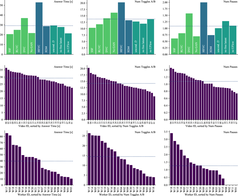
Figure 9: User study statistics, grouped in various ways. The dotted line in each plot indicates the mean of the values shown in the plot. From left to right, we show different statistics: Answer time in [s]econds, number of flips, and number of pauses. The rows show different ways of grouping the data: Top: We group by study, and color based on whether the study compares to a neural codec, to a standard codec, or is an ablation. Middle: We group by MCL-JCV video ID (01 to 30), and sort each plot. Bottom: We group by rater ID, and sort each plot (note that the means here are slightly different, as not all raters rate did the same number of studies).

0.A.3 Decoupled Scale-Space Warping: Details

Figure 10: Numpy implementation of adaptive blurring.

We show a numpy version of adaptive blurring in Fig. 10, and a visualization of some variables in Fig. 12. To validate our implementation of decoupled scale-space warping (DSSW), we compare MSE-trained models in Fig. 11. We show that DSSW with bilinear warping is similar to scale-space warping with trilinear interpolation, validating our version. We see that using a bicubic resampling kernel, R-D performance improves by ${\approx}6\%$. As we mention in Sec. 3.2, DSSW is also significantly faster to run on GPU. For the Figure, we used the architecture of [1] trained for MSE only, with a slightly accelerated training schedule by skipping the last training stage on larger (384px) crops, instead decaying the learning rate by 10x after 800 000 steps.

Figure 11: To validate our Decoupled Scale Space Warping (DSSW) implementation, we train models for MSE. We compare the R-D performance of Bilinear/Bicubic resamplers in DSSW against the Scale-Space Warping of Agustsson et al. [1] and find that DSSW with bicubic improves the bpp. We also show plain bilinear warping, without any scale space blurring.

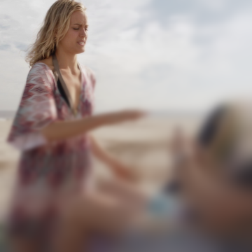
image	sigma_field	adaptive_blur(image,
		xxxxxxxxxxxxxxsigma_field)
coeffs_by_level[level]
level = 0	level = 2	level = 4
coeffs_by_level[level] * scale_space_volume(image, sigmas[level])
level = 0	level = 2	level = 4

Figure 12: Visualizing variables of the algorithm given in Fig. 10.

0.A.4 DVC Details

To get DVC reconstructions, we use the code provided by the authors. DVC uses the image compression model by Ballé et al. [5] for I-frames, but the code does not include the exact model. We thus tried all models, and picked the one with highest R-D performance, which is available as “bmshj2018-hyperprior-mse-5” in TFC.. We note that we add padding and cropping as described in Sec. 4.3. We show the PSNR of our model obtained on UVG in Fig. 13.

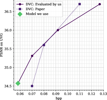
Figure 13: Comparing our DVC models to what the authors reported, on UVG. We use the model in the lower right, as this is closest to our bpps (achieving $\approx 0.06$bpp on UVG, $\approx 0.09$bpp on MCL-JCV).

0.A.5 Architecture Details

A detailed version of the architecture from Fig. 3 is given in Fig. 14.

0.A.6 Hyper Parameters

For scale space blurring we set $\sigma_{0}=1.5$ and used $L=6$ levels, which implies that the sequence of blur kernel sizes is $[0.0,1.5,3.0,6.0,12.0,24.0]$.

For rate control we initially swept over a wide range $k_{P}\in\{10^{i},i\in\{-1,\dots,-9\}\}$ and found that $10^{-3}$ worked well, which we then fixed for all future experiments. We initialized $\log_{2}\lambda_{R}=1.0$ in all cases.

Previous works [27, 24] typically initially train for a higher bitrate. This is usually implemented by using a schedule on the R-D weight $\lambda$ that is decayed by a factor $2\times$ or $10\times$ early in training. Since the rate-controllor automatically controls this weight, we emulate the approach by instead using a schedule on the targeted bitrate $b_{t}$. We use a simple rule and target a $+0.5$ higher bitrate for the first $20\%$ of training steps.

For the I-frame loss $\mathcal{L}_{\textit{I-Frame}}$ (Eq. 6), we use $\beta=128$, and $b_{t}=0.4$ for rate-control.

For the P-frame loss $\mathcal{L}_{\textit{P-Frame}}$ (Eq. 8), we use $\beta=128$, and $k_{\text{TV}}=10.0,k_{\text{flow}}=1.0$ in $\mathcal{L}_{\text{reg}}$. For the three different models we use in the user study, we use $b_{t}\in\{0.05,0.10,0.15\}$. A detail omitted from the equation is that we scale the loss by the constant $C_{T}=1/T\sum_{t=2}^{T}t$, as this yields similar magnitudes as no loss scaling.

We use the same learning rate $\text{LR}=1\textsc{e}{-4}$ for all networks, and train with the Adam optimizer. We linearly increase the LR from 0 during the first $20k$ steps, and then drop it to $\text{LR}=1\textsc{e}{-5}$ after $320k$ steps. We train the discriminators for 1 step for each generator training step.

0.A.7 Training Time

In Table 3 we report the training speed for each of the training stages, which results in a total training time of ${\approx}48$ hours. We note that the first stage (I-frame) trains more than $14{\times}$ faster than the last stage in terms of steps/s.

Batch size	#I	#P	# steps [k]	steps/s	time [h]
8	1	0	1 000 000	19.7	14.1
8	1	1	80 000	7.3	3.0
8	1	2	220 000	3.9	15.7
8	1	3	50 000	2.6	5.3
8	1	5	50 000	1.4	9.9
Totals:			1 400 000		48.0

Table 3: Training speed/time for each stage of our model on a Google Cloud TPU. #I, #P indicates the number of I- resp. P-frames used in that stage.

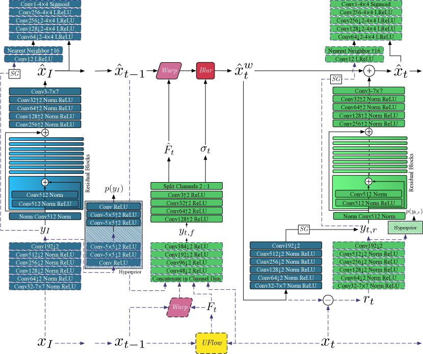
Figure 14: Detailed view of the architecture, showing the layers in each of the blocks in Fig. 3. “Conv$F$” denotes a 2D convolution with $F$ output channels, “-S$\times$S” denots the filter size, if that is omitted we use 3${\times}$3. ${\downarrow}2$, ${\uparrow}2$ indicates downsampling and upsampling, respectively, “Norm” is the ChannelNorm layer employed by HiFiC [24]. The blocks with a color gradient are Residual Blocks, we only show the detail in one. “LReLU” is the Leaky ReLU with $\alpha=0.2$. We note that we employ SpectralNorm in both discriminators. The distributions predicted by the Hyperprior are used to encode the latents with entropy coding. Like in Fig. 3, learned I-frame CNNs are in blue, learned P-frame CNNs in green, dashed lines are not active during decoding, SG is a stop gradient operation, Blur is scale space blurring, Warp is bicubic warping. UFlow is a frozen optical flow model from [18].

Appendix 0.B Data Release

0.B.1 CSVs and Reconstructions

For each user study comparison we made between methods, we release the reconstructions as well as a CSV containing all the rater information, via anonymous links, see Table. 4.

1. Reconstructions folders:

   1. Folder per method, which contains a subfolder for each of the 30 videos of MCL-JCV, and each such video subfolder contains 60 PNGs, the reconstructions of the resp. method.

2. CSVs: For each study, we release a CSV, where:

   1. Each row is a video, and we have the following columns: wins_left, wins_right indicate the number of times each method won (left is always Ours), bpp_left, bpp_right, indicate the per-video bpps, avg_flips, avg_answer_time_ms, avg_num_pauses indicate average flips, average time per video, and average num pauses, respectively.

1. https://storage.googleapis.com/eccv_sub/csvs.zip

2. https://storage.googleapis.com/eccv_sub/ours.zip

3. https://storage.googleapis.com/eccv_sub/nogan.zip

4. https://storage.googleapis.com/eccv_sub/ssf.zip

5. https://storage.googleapis.com/eccv_sub/h264.zip

6. https://storage.googleapis.com/eccv_sub/hevc.zip

Table 4: Links to user study data.

0.B.2 Tables

We show wins per method per video, that are available in the CSVs, in Table 5.

video	Ours	No-GAN	Ours	SSF	Ours	DVC	Ours	RLVC	Ours	H264	Ours	HEVC
01	4	4	5	4	10	1	6	3	6	2	4	6
02	4	4	7	1	10	0	4	4	2	6	3	7
03	7	2	7	1	11	0	6	2	7	2	7	3
04	5	3	5	3	11	0	5	3	8	0	8	2
05	6	2	7	1	9	1	6	3	7	2	6	4
06	3	5	5	4	7	3	6	3	4	4	8	2
07	7	1	7	1	12	0	6	2	7	1	8	2
08	7	1	7	2	10	1	6	3	5	4	9	1
09	4	4	8	2	6	5	6	3	6	2	7	3
10	5	3	8	1	8	3	7	2	5	3	2	8
11	7	1	5	3	10	1	7	2	5	3	6	4
12	7	1	7	1	11	0	5	3	4	4	7	3
13	5	3	3	5	9	2	4	5	4	5	8	2
14	6	2	7	2	9	2	7	2	6	2	8	2
15	7	2	8	1	8	2	7	3	7	1	8	2
16	4	4	7	2	9	2	5	4	6	2	8	2
17	4	4	5	3	10	2	6	2	7	1	9	1
18	5	3	6	2	10	1	7	2	6	3	6	4
19	7	2	8	1	8	2	8	1	5	3	6	4
20	6	2	3	6	10	0	8	0	1	8	3	7
21	3	5	4	5	8	3	6	3	4	4	3	7
22	5	3	5	3	9	3	5	4	6	2	7	3
23	5	3	7	2	10	1	8	2	6	2	8	2
24	5	3	6	2	10	1	6	4	5	3	2	8
25	6	2	8	1	8	3	5	5	5	3	5	5
26	4	4	6	2	8	2	8	1	4	5	7	3
27	8	0	7	1	10	1	6	3	7	1	8	2
28	7	1	7	1	9	2	6	3	8	0	5	5
29	7	1	5	4	7	4	5	4	2	7	2	8
30	5	3	8	1	9	1	7	2	6	2	6	4
	165	78	188	68	276	49	184	83	161	87	184	116

Table 5: Wins per method for our user studies.

References

- [1] Agustsson, E., Minnen, D., Johnston, N., Balle, J., Hwang, S.J., Toderici, G.: Scale-space flow for end-to-end optimized video compression. In: Proceedings of the IEEE/CVF Conference on Computer Vision and Pattern Recognition. pp. 8503–8512 (2020)
- [2] Agustsson, E., Tschannen, M., Mentzer, F., Timofte, R., Gool, L.V.: Generative adversarial networks for extreme learned image compression. In: The IEEE International Conference on Computer Vision (ICCV) (October 2019)
- [3] Ahmed, N., Natarajan, T., Rao, K.R.: Discrete cosine transform. IEEE Trans. on Computers C-23(1) (1974). https://doi.org/10.1109/T-C.1974.223784
- [4] ITU-T rec. H.264 & ISO/IEC 14496-10 AVC: Advanced video coding for generic audiovisual services (2003)
- [5] Ballé, J., Minnen, D., Singh, S., Hwang, S.J., Johnston, N.: Variational image compression with a scale hyperprior. In: International Conference on Learning Representations (ICLR) (2018)
- [6] Bankoski, J., Wilkins, P., Xu, Y.: Technical overview of vp8, an open source video codec for the web. In: 2011 IEEE International Conference on Multimedia and Expo. pp. 1–6. IEEE (2011)
- [7] Blau, Y., Michaeli, T.: The perception-distortion tradeoff. In: Proceedings of the IEEE Conference on Computer Vision and Pattern Recognition (CVPR) (June 2018)
- [8] Blau, Y., Michaeli, T.: Rethinking lossy compression: The rate-distortion-perception tradeoff. arXiv preprint arXiv:1901.07821 (2019)
- [9] Chen, Y., Murherjee, D., Han, J., Grange, A., Xu, Y., Liu, Z., Parker, S., Chen, C., Su, H., Joshi, U., et al.: An overview of core coding tools in the av1 video codec. In: 2018 Picture Coding Symposium (PCS). pp. 41–45. IEEE (2018)
- [10] Djelouah, A., Campos, J., Schaub-Meyer, S., Schroers, C.: Neural inter-frame compression for video coding. In: Proceedings of the IEEE/CVF International Conference on Computer Vision. pp. 6421–6429 (2019)
- [11] Golinski, A., Pourreza, R., Yang, Y., Sautiere, G., Cohen, T.S.: Feedback recurrent autoencoder for video compression. In: Proceedings of the Asian Conference on Computer Vision (2020)
- [12] Goodfellow, I., Pouget-Abadie, J., Mirza, M., Xu, B., Warde-Farley, D., Ozair, S., Courville, A., Bengio, Y.: Generative adversarial nets. In: Advances in neural information processing systems. pp. 2672–2680 (2014)
- [13] Google AI platform data labeling service. https://cloud.google.com/ai-platform/data-labeling/pricing, accessed: 2021-05-01
- [14] Goyal, V.K.: Theoretical foundations of transform coding. IEEE Signal Processing Magazine 18(5) (2001). https://doi.org/10.1109/79.952802
- [15] Habibian, A., Rozendaal, T.v., Tomczak, J.M., Cohen, T.S.: Video compression with rate-distortion autoencoders. In: Proceedings of the IEEE/CVF International Conference on Computer Vision. pp. 7033–7042 (2019)
- [16] Heusel, M., Ramsauer, H., Unterthiner, T., Nessler, B., Hochreiter, S.: Gans trained by a two time-scale update rule converge to a local nash equilibrium. In: Advances in Neural Information Processing Systems. pp. 6626–6637 (2017)
- [17] ITU-T rec. H.265 & ISO/IEC 23008-2: High efficiency video coding (2013)
- [18] Jonschkowski, R., Stone, A., Barron, J.T., Gordon, A., Konolige, K., Angelova, A.: What matters in unsupervised optical flow. arXiv preprint arXiv:2006.04902 1(2), 3 (2020)
- [19] Krizhevsky, A., Sutskever, I., Hinton, G.E.: Imagenet classification with deep convolutional neural networks. In: Advances in neural information processing systems. pp. 1097–1105 (2012)
- [20] Li, J., Li, B., Lu, Y.: Deep contextual video compression. Advances in Neural Information Processing Systems 34, 18114–18125 (2021)
- [21] Liu, H., Chen, T., Lu, M., Shen, Q., Ma, Z.: Neural video compression using spatio-temporal priors. arXiv preprint arXiv:1902.07383 (2019)
- [22] Liu, J., Wang, S., Ma, W.C., Shah, M., Hu, R., Dhawan, P., Urtasun, R.: Conditional entropy coding for efficient video compression. arXiv preprint arXiv:2008.09180 (2020)
- [23] Lu, G., Ouyang, W., Xu, D., Zhang, X., Cai, C., Gao, Z.: Dvc: An end-to-end deep video compression framework. In: Proceedings of the IEEE/CVF Conference on Computer Vision and Pattern Recognition. pp. 11006–11015 (2019)
- [24] Mentzer, F., Toderici, G.D., Tschannen, M., Agustsson, E.: High-fidelity generative image compression. Advances in Neural Information Processing Systems 33 (2020)
- [25] Mercat, A., Viitanen, M., Vanne, J.: UVG dataset: 50/120fps 4K sequences for video codec analysis and development. In: Proceedings of the 11th ACM Multimedia Systems Conference. pp. 297–302 (2020)
- [26] Minnen, D., Ballé, J., Toderici, G.D.: Joint autoregressive and hierarchical priors for learned image compression. In: Advances in Neural Information Processing Systems. pp. 10771–10780 (2018)
- [27] Minnen, D., Singh, S.: Channel-wise autoregressive entropy models for learned image compression. arXiv preprint arXiv:2007.08739 (2020)
- [28] Mirza, M., Osindero, S.: Conditional generative adversarial nets. arXiv preprint arXiv:1411.1784 (2014)
- [29] Mukherjee, D., Bankoski, J., Grange, A., Han, J., Koleszar, J., Wilkins, P., Xu, Y., Bultje, R.: The latest open-source video codec vp9-an overview and preliminary results. In: 2013 Picture Coding Symposium (PCS). pp. 390–393. IEEE (2013)
- [30] Nehab, D., Hoppe, H., et al.: A fresh look at generalized sampling. Citeseer (2014)
- [31] Netflix: VMAF - Video Multi-Method Assessment Fusion. https://github.com/Netflix/vmaf/
- [32] Platt, J.C., Barr, A.H.: Constrained differential optimization for neural networks. Caltech (1988)
- [33] Rippel, O., Anderson, A.G., Tatwawadi, K., Nair, S., Lytle, C., Bourdev, L.: ELF-VC: Efficient Learned Flexible-Rate Video Coding. arXiv preprint arXiv:2104.14335 (2021)
- [34] Rippel, O., Bourdev, L.: Real-time adaptive image compression. In: Proceedings of the 34th International Conference on Machine Learning. Proceedings of Machine Learning Research, vol. 70, pp. 2922–2930. PMLR, International Convention Centre, Sydney, Australia (06–11 Aug 2017)
- [35] Rippel, O., Nair, S., Lew, C., Branson, S., Anderson, A.G., Bourdev, L.: Learned video compression. In: Proceedings of the IEEE/CVF International Conference on Computer Vision. pp. 3454–3463 (2019)
- [36] van Rozendaal, T., Sautiere, G., Cohen, T.S.: Lossy compression with distortion constrained optimization. In: Proceedings of the IEEE/CVF Conference on Computer Vision and Pattern Recognition Workshops. pp. 166–167 (2020)
- [37] Santurkar, S., Budden, D., Shavit, N.: Generative compression. arXiv preprint arXiv:1703.01467 (2017)
- [38] Shulman, D., Herve, J.Y.: Regularization of discontinuous flow fields. In: Proc. workshop on visual motion. pp. 81–86. IEEE Computer Society Press (1989)
- [39] Theis, L., Agustsson, E.: On the advantages of stochastic encoders. arXiv preprint arXiv:2102.09270 (2021)
- [40] Theis, L., Wagner, A.B.: A coding theorem for the rate-distortion-perception function. arXiv preprint arXiv:2104.13662 (2021)
- [41] Toderici, G., Theis, L., Johnston, N., Agustsson, E., Mentzer, F., Ballé, J., Shi, W., Timofte, R.: CLIC 2020: Challenge on Learned Image Compression (2020), http://compression.cc
- [42] Tschannen, M., Agustsson, E., Lucic, M.: Deep generative models for distribution-preserving lossy compression. In: Advances in Neural Information Processing Systems. pp. 5929–5940 (2018)
- [43] Wang, H., Gan, W., Hu, S., Lin, J.Y., Jin, L., Song, L., Wang, P., Katsavounidis, I., Aaron, A., Kuo, C.C.J.: MCL-JCV: a JND-based H.264/AVC video quality assessment dataset. In: 2016 IEEE International Conference on Image Processing (ICIP). pp. 1509–1513. IEEE (2016)
- [44] Wang, T.C., Liu, M.Y., Zhu, J.Y., Liu, G., Tao, A., Kautz, J., Catanzaro, B.: Video-to-video synthesis. In: Advances in Neural Information Processing Systems (NeurIPS) (2018)
- [45] Wang, Z., Simoncelli, E.P., Bovik, A.C.: Multiscale structural similarity for image quality assessment. In: The Thrity-Seventh Asilomar Conference on Signals, Systems & Computers, 2003. vol. 2, pp. 1398–1402. Ieee (2003)
- [46] Wu, C.Y., Singhal, N., Krahenbuhl, P.: Video compression through image interpolation. In: Proceedings of the European Conference on Computer Vision (ECCV). pp. 416–431 (2018)
- [47] Yang, R., Mentzer, F., Van Gool, L., Timofte, R.: Learning for video compression with recurrent auto-encoder and recurrent probability model. IEEE Journal of Selected Topics in Signal Processing (2020)
- [48] Yang, R., Yang, Y., Marino, J., Mandt, S.: Hierarchical autoregressive modeling for neural video compression. arXiv preprint arXiv:2010.10258 (2020)
- [49] Yang, Y., Mandt, S., Theis, L.: An introduction to neural data compression. arXiv preprint arXiv:2202.06533 (2022)
- [50] YouTube Data API (2021), https://www.googleapis.com/youtube/v3/videoCategories
- [51] Zhang, R., Isola, P., Efros, A.A., Shechtman, E., Wang, O.: The unreasonable effectiveness of deep features as a perceptual metric. In: Proceedings of the IEEE Conference on Computer Vision and Pattern Recognition. pp. 586–595 (2018)