ContextNet: A Click-Through Rate Prediction Framework Using Contextual information to Refine Feature Embedding

Abstract.

Click-through rate (CTR) estimation is a fundamental task in personalized advertising and recommender systems and it’s important for ranking models to effectively capture complex high-order features. Inspired by the success of ELMO and Bert in NLP field, which dynamically refine word embedding according to the context sentence information where the word appears, we think it’s also important to dynamically refine each feature’s embedding layer by layer according to the context information contained in input instance in CTR estimation tasks. We can effectively capture the useful feature interactions for each feature in this way. In this paper, We propose a novel CTR Framework named ContextNet that implicitly models high-order feature interactions by dynamically refining each feature’s embedding according to the input context. Specifically, ContextNet consists of two key components: contextual embedding module and ContextNet block. Contextual embedding module aggregates contextual information for each feature from input instance and ContextNet block maintains each feature’s embedding layer by layer and dynamically refines its representation by merging contextual high-order interaction information into feature embedding. To make the framework specific, we also propose two models(ContextNet-PFFN and ContextNet-SFFN) under this framework by introducing linear contextual embedding network and two non-linear mapping sub-network in ContextNet block. We conduct extensive experiments on four real-world datasets and the experiment results demonstrate that our proposed ContextNet-PFFN and ContextNet-SFFN model outperform state-of-the-art models such as DeepFM and xDeepFM significantly.

1. Introduction

Click-through rate (CTR) estimation has become one of the most essential tasks in many real-world applications. Many models have been proposed to resolve this problem such as Logistic Regression (LR) (McMahan et al., 2013), Polynomial-2 (Poly2) (Rendle, 2010), tree-based models (He et al., 2014), tensor-based models (Koren et al., 2009), Bayesian models (Graepel et al., 2010), and Field-aware Factorization Machines (FFMs) (Juan et al., 2016).

Deep learning techniques have shown promising results in many research fields such as computer vision (Krizhevsky et al., 2012; He et al., 2016), speech recognition (Graves et al., 2013; Tang et al., 2017) and natural language understanding (Cho et al., 2014; Mikolov et al., 2010). As a result, employing DNNs for CTR estimation has also been a research trend in this field (Zhang et al., 2016; Cheng et al., 2016; Xiao et al., 2017; Guo et al., 2017; Lian et al., 2018; Qu et al., 2016; Wang et al., 2017). Some deep learning based models have been introduced and achieved success such as Factorisation-Machine Supported Neural Networks(FNN)(Zhang et al., 2016), Attentional Factorization Machine (AFM)(Cheng et al., 2016), wide&deep(Xiao et al., 2017), DeepFM(Guo et al., 2017), xDeepFM (Lian et al., 2018), DIN(Zhou et al., 2018) etc.

Feature interaction is critical for CTR tasks and it’s important for these ranking models to effectively capture complex features. Most DNN ranking models such as FNN and DeepFM use the shallow MLP layers to model high-order interactions in implicit way which has been proved to be ineffective (Beutel et al., 2018b). Some CTR model like xDeepFM (Lian et al., 2018) explicitly introduces high-order feature interactions by adding sub-network into the network structure. However, that will significantly increases the computation time and it’s hard to deploy it in real-world application.

Inspired by the success of ELMO(Peters et al., 2018) and Bert(Devlin et al., 2018) in NLP field, which dynamically refine word embedding according to the sentence context where the word appears, we think it’s also important to dynamically change the feature embedding according to other contextual features in the same instance it appears in CTR tasks. We can effectively capture the useful feature interactions for each feature by introducing the context aware feature embedding into CTR models.

Though AutoInt(Song et al., 2019) and Fi-GNN(Li et al., 2019) can also dynamically change feature embedding as our proposed model does, feature representation of these models is kind of weighted summation of pair-wise interaction . These models follow the rule of feature aggregation in summation way after pair-wise interaction, while our proposed model follow the rule of feature interaction in multiplicative way after feature aggregation by a specific network. Alex Beutel et.al(Beutel et al., 2018a) have proved that addictive feature interaction is inefficient in capturing common feature crosses. They proposed a simple but effective approach named “latent cross” which is a kind of multiplicative interactions between the context embedding and the neural network hidden states in RNN model. Our work is inspired by both the Bert and “latent cross”.

In this work, We propose a new CTR framework named ContextNet which can dynamically refine feature’s embedding according to the context it appears and effectively model high-order feature interactions for each feature. Specifically, ContextNet consists of two key components: contextual embedding module and ContextNet block. Contextual embedding module aggregates contextual information for each feature from input instance and ContextNet block maintains each feature’s embedding layer by layer and dynamically refines its representation by merging contextual high-order interaction information into feature embedding. So the ContextNet provides a flexible mechanism for each feature to dynamically and efficiently filter out the most useful high-order cross information for its own purpose in current context it appears. Another advantage of ContextNet over most DNN models is that it has good model interpretability. Notice that ContextNet is a new CTR framework instead of a specific model, which means we can design various detailed models based on this framework. We also propose two ContextNet based models in this paper in order to make the ContextNet framework specific and experimental results prove its effectiveness.

The contributions of our work are summarized as follows:

1. We propose a novel CTR Framework named ContextNet that implicitly models high-order feature interactions by dynamically refining the feature embedding according to the context information contained in input instance.

2. To make the ContextNet framework specific, we propose a contextual embedding network and two non-linear mapping sub-network in ContextNet block. So we design two specific ContextNet-based models in our work under the proposed framework, which is named ContextNet-PFFN and ContextNet-SFFN, respectively.

3. We conduct extensive experiments on four real-world datasets and the experiment results demonstrate that our proposed ContextNet-PFFN and ContextNet-SFFN outperform state-of-the-art models significantly.

The rest of this paper is organized as follows. Section 2 introduces some related works which are relevant with our proposed model. We introduce our proposed ContextNet framework in detail in Section 3. The experimental results on four real world datasets are presented and discussed in Section 4. Section 5 concludes our work in this paper.

2. Related Work

2.1. Context Aware Word Embedding in NLP

Word embedding is a very important concept in NLP and it attempts to map words from a discrete space into a semantic space. In early stage, Word2vec(Mikolov et al., 2013) and GloVe(Pennington et al., 2014) learn a constant embedding vector for a word and the embedding is same for a word in different sentences. However, it’s obvious that polysemous word should have different embedding in various sentence contexts. To deal with this issue, context information of the sentence is used to predict a dynamic word embedding. For example, ELMO(Peters et al., 2018) uses the bidirectional RNN to model the context information. The GPT(Radford et al., 2018) and Bert(Devlin et al., 2018) model leverages the Transformer(Vaswani et al., 2017) model to jointly consider both the left and right context information in the sentence. Our work is inspired by these context aware word embedding approaches and we introduce context aware feature embedding into CTR tasks in this work.

2.2. Deep Learning based CTR Models

Many deep learning based CTR models have been proposed in recent years and how to effectively model the feature interactions is the key factor for most of these neural network based models.

Factorization-Machine Supported Neural Networks (FNN)(Zhang et al., 2016) is a feed-forward neural network using FM to pre-train the embedding layer. Wide & Deep Learning(Xiao et al., 2017) jointly trains wide linear models and deep neural networks to combine the benefits of memorization and generalization for recommender systems. However, expertise feature engineering is still needed on the input to the wide part of Wide & Deep model. To alleviate manual efforts in feature engineering, DeepFM(Guo et al., 2017) replaces the wide part of Wide & Deep model with FM and shares the feature embedding between the FM and deep component. Most DNN CTR models rely on two or three MLP layers to model the high-order interactions in an implicit way and some research(Beutel et al., 2018b) has proved MLP is an ineffective way to capture the high-order interactions.

Some works explicitly introduce high-order feature interactions by sub-network. Deep & Cross Network (DCN)(Wang et al., 2017) efficiently captures feature interactions of bounded degrees in an explicit fashion. Similarly, eXtreme Deep Factorization Machine (xDeepFM) (Lian et al., 2018) also models the low-order and high-order feature interactions in an explicit way by proposing a novel Compressed Interaction Network (CIN) part. FiBiNET(Huang et al., 2019) can dynamically learn feature importance via the Squeeze-Excitation network (SENET) mechanism and feature interactions via bilinear function. AutoInt(Song et al., 2019) proposes a multi-head self-attentive neural network with residual connections to explicitly model the feature interactions in the low-dimensional space. Fi-GNN(Li et al., 2019) represents the multi-field features in a graph structure, where each node corresponds to a feature field and different fields can interact through edges. Though AutoInt[25] and Fi-GNN(Li et al., 2019) can also dynamically change feature embedding by proposing a multi-head self-attentive neural network or graph neural network, feature representation of these models is kind of weighted summation of pair-wise interaction. Many research(Beutel et al., 2018a; Rendle et al., 2020) have proved that addictive feature interaction is inefficient in capturing common feature crosses. Our proposed models collect global contextual information by an independent contextual embedding network to change the feature representation in the multiplicative way. Our experimental results show this advantage.

3. Our Proposed Model

In this section, we will firstly introduce ContextNet framework and then describe the key components in detail in the following sections.

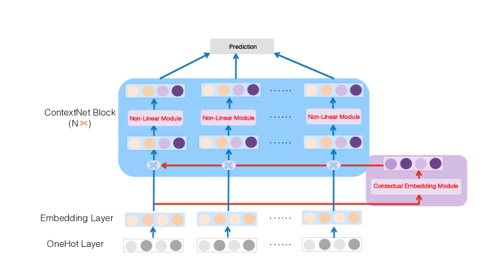
Figure 1. The Neural Structure of ContextNet Framework

3.1. ContextNet Framework

As depicted in Figure 1, we propose a novel CTR Framework named ContextNet that implicitly models high-order feature interactions by dynamically refining the feature embedding according to the context information contained in input instance. ContextNet consists of two variable components: contextual embedding module and ContextNet block. Contextual embedding module aggregates contextual information in the same instance for each feature and projects the collected contextual information to the same low-dimensional space as feature embedding lies in. Notice that the input of contextual embedding module is always from the feature embedding layer. ContextNet block implicitly model high-order interactions by merging contextual information into each feature’s feature embedding firstly, and then conduct the non-linear transformation on the merged embedding in order to better capture high-order interactions. We can stack ContextNet block by block to form deeper network and the refined feature’s embedding output of the previous block is the input of the next one. The different ContextNet block has the corresponding contextual embedding module to refine each feature’s embedding. The final ContextNet block’s output is feed into the prediction layer to give the instance’s prediction value.

3.2. Feature Embedding

The input data of CTR tasks usually consists of sparse and dense features. Such features are encoded as one-hot vectors which often lead to excessively high-dimensional feature spaces for large vocabularies. The common solution to this problem is to introduce the embedding layer. Generally, the sparse input can be formulated as:

(1) $$x=[x_{1},x_{2},...,x_{f}]$$

where $f$ denotes the number of fields, and $x_{i}\in\mathbb{R}^{n}$ denotes a one-hot vector for a categorical field with $n$ features and $x_{i}\in\mathbb{R}^{n}$ is vector with only one value for a numerical field. We can obtain feature embedding $E_{i}$ for one-hot vector $x_{i}$ via:

(2) $$E_{i}=W_{e}x_{i}$$

where $W_{e}\in\mathbb{R}^{k\times n}$ is the embedding matrix of $n$ features and $k$ is the dimension of field embedding. The numerical feature $x_{j}$ can also be converted into the same low-dimensional space by:

(3) $$E_{j}=V_{j}x_{j}$$

where $V_{j}\in\mathbb{R}^{k}$ is the corresponding field embedding with size $k$.

Through the aforementioned method, an embedding layer is applied upon the raw feature input to compress it to a low dimensional, dense real-value vector. The result of embedding layer is a wide concatenated vector:

(4) $$E=concat(E_{1},E_{2},...,E_{i},...,E_{f})$$

where $f$ denotes the number of fields, and $E_{i}\in\mathbb{R}^{k}$ denotes the embedding of one field. Although the feature lengths of instances can be various, their embeddings are of the same length $f\times k$, where $k$ is the dimension of field embedding.

3.3. Contextual Embedding

As discussed in Section 3.1, the contextual embedding module in ContextNet has two objectives: Firstly, ContextNet use this module to aggregate contextual information for each feature from input instance, that is to say, feature embedding layer. Secondly, the collected contextual information for one feature is projected to the same low-dimensional space as feature embedding lies in.

We can formulate this process as follows:

(5) $$CE_{i}=\mathcal{F}_{project}(\mathcal{F}_{agg}(E_{i},E;\Theta_{a});\Theta_{p})$$

where $CE_{i}\in\mathbb{R}^{k}$ denotes the contextual embedding of the $i$-th feature $E_{i}$ and $k$ is the dimension of field embedding, $\mathcal{F}_{agg}(E_{i},E;\Theta_{a})$ is the contextual information aggregation function for the $i$-th feature field which uses the embedding layer $E$ and feature embedding $E_{i}$ as input and $\Theta_{a}$ denotes the parameters of aggregation model. $\mathcal{F}_{project}(F_{agg};\Theta_{p})$ is the mapping function to project the contextual information into the same low-dimensional space with feature embedding lies in. $\Theta_{p}$ denotes the parameters of projection model.

To make this module more specific, We propose a two-layer contextual embedding network (TCE) for this module in our paper. That is to say, we adapt the feed forward network as the aggregation function $\mathcal{F}_{agg}(E_{i},E;\Theta_{a})$ and projection function $\mathcal{F}_{project}(F_{agg};\Theta_{p})$. Notice here that TCE is just a specific solution for this module and there are other options that deserve further exploration. However, the input of the contextual embedding module should be from embedding layer which contains original and global contextual information.

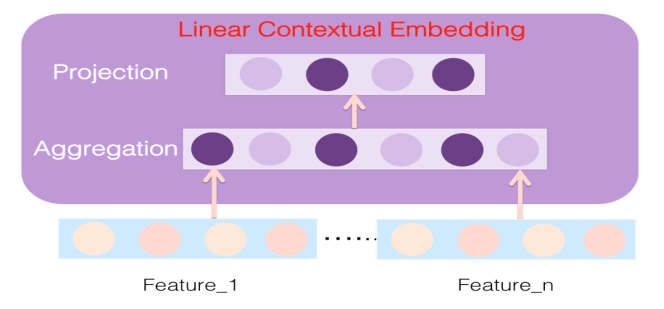
Figure 2. Two Layer Contextual Embedding

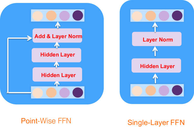
Figure 3. Structure of Non-Linear Transformation

Next we will describe how contextual embedding network works. Suppose we have a feature $E_{i}$ which belongs to feature field $d$. As depicted in Figure 3, two fully connected (FC) layers are used in TCE module. The first FC layer is called ”aggregation layer” which is a relatively wider layer to collect the contextual information from embedding layer with parameters $W^{a}_{d}$. The second FC layer is ”projection layer” which projects the contextual information into the same low-dimension space with feature embedding and reduces dimensionality to the same size as feature embedding has. The projection layer has parameter $W_{d}^{p}$. Formally,

(6) $$CE_{i}=\mathcal{F}_{project}(\mathcal{F}_{agg}(E_{i},E;\Theta_{a});\Theta_{p})=W_{d}^{p}(RELU(W_{d}^{a}E))$$

where $E\in\mathbb{R}^{m=f\times k}$ refers to the embedding layer of input instance, $W_{d}^{a}\in\mathbb{R}^{t\times m}$ and $W_{d}^{p}\in\mathbb{R}^{k\times t}$ are parameters for aggregation and projection layer in TCE for field $d$, respectively. $t$ and $k$ respectively denotes the neural number of aggregation and projection layer. Notice here that the aggregation layer is usually wider than the projection layer because the size of the projection layer is required to be equal to the feature embedding size $k$. The wider aggregation layer will make the model be more expressive.

We can see from formula (6) that each feature field $d$ maintains its own parameters $W_{d}^{a}$ and $W_{d}^{p}$ for aggregation and projection layer, respectively. Suppose we have $f$ different feature fields in embedding layer, the parameter number of TCE will be $f\ast(W_{d}^{a}+W_{d}^{p})$. We can reduce parameter number by sharing $W_{d}^{a}$ in aggregation layer among all fields. The parameter number of TCE will be reduce to $W_{d}^{a}+f\ast W_{d}^{p}$. In order to reduce the model parameters, we adopt the following strategy: we share the parameters of aggregation layer among all feature fields while keep the parameters of projection layer private for each feature field. This strategy effectively balances the model complexity and the model’s expressive ability because the private projection layer will make each feature extract useful contextual information for its purpose independently. This makes the TCE module look like the ”share-bottom” structure in multi-task learning where the bottom hidden layers are shared across tasks as works (Caruana, 1997) and (Caruana, 1993) did.

3.4. ContextNet Block

As discussed in Section 3.1, ContextNet block is used to dynamically refine each feature’s embedding by merging the contextual embedding produced for that feature to implicitly capture the high-order feature interactions. To achieve this goal, there are two consequential procedures in ContenxtNet block as shown in Figure 1: embedding merging and a following non-linear transformation. We can stack ContextNet block by block to form deep network and the output of the previous block is the input of the next block.

Next we will describe how ContextNet block works. We use $E_{i}^{l}$ to denote the output feature embedding of the $l$-th block, that is to say, $E_{i}^{l}$ is the input embedding of the $i$-th feature for the $(l+1)$-th block. $CE_{i}^{l+1}$ denotes the corresponding contextual embedding computed by TCE for the $i$-th feature field in the $(l+1)$-th block.

We can describe this process for the $i$-th feature as follows:

(7) $$E_{i}^{l+1}=\mathcal{F}_{non-linear}(\mathcal{F}_{merge}(E_{i}^{l},CE_{i}^{l+1};\Theta_{m});\Theta_{n})$$

where $E_{i}^{l+1}\in\mathbb{R}^{k}$ denotes the fine-tuned feature embedding outputted by the $(l+1)$-th ContextNet block for the $i$-th feature $E^{l}_{i}$ and $k$ is the dimension of field embedding, $\mathcal{F}_{merge}(E_{i}^{l},CE_{i}^{l+1};\Theta_{m})$ is the merging function for the $i$-th feature which uses the previous block’s output feature embedding $E_{i}^{l}$ and contextual embedding $CE_{i}^{l+1}$ in current block as input. $\Theta_{m}$ denotes the parameters pf merging function. $\mathcal{F}_{non-linear}(F_{merge};\Theta_{n})$ is the mapping function to conduct the non-linear transformation on the merged embedding in order to further capture high-order interactions for the $i$-th feature. $\Theta_{n}$ denotes the parameters of non-linear transformation function.

As for the merging function $F_{merge}(E_{i}^{l},CE^{l+1}_{i};\Theta_{m})$, Hadamard product is used in this work to merge the feature embedding $E_{i}^{l}$ and the corresponding contextual embedding $CE_{i}^{l+1}$ as follows:

(8) $$E_{i}^{l}\otimes CE_{i}^{l+1}=\left[E_{i1}^{l}\cdot CE_{i1}^{l+1},...,E_{ij}^{l}\cdot CE_{ij}^{l+1},...,E_{ik}^{l}\cdot CE_{ik}^{l+1}\right]$$

where $k$ is the size of embedding vector $E_{i}^{l}$ and contextual embedding $CE_{i}^{l+1}$ for the $i$-th feature. Hadamard product is a kind of element-wise production operation without parameters.

As for the non-linear function $F_{non-linear}(F_{merge};\Theta_{n})$, we propose two neural networks which are shown in Figure 3 in this paper: point-wise feed-forward network and single-layer feed-forward network.

Point-Wise Feed-Forward Network:

Though the ContextNet uses the contextual embedding module to aggregate all other feature’s embedding and then project them to a fixed embedding size, ultimately it is still a linear model. For endowing the model with nonlinearity in order to capture high-order interactions better, we can apply a point-wise two-layer feed-forward network to all $E_{i}$ identically (sharing parameters among all feature field):

(9) $$\mathcal{F}_{i}=PFFN(E_{i};\Theta_{n})=LN(RELU(E_{i}W^{1})W^{2}+E_{i})$$

where $W^{1}$, $W^{2}$ are $k\times k$ matrices and $k$ is the dimension of field embedding. We also adapt the residual connection and layer normalization ($LN$) (Ba et al., 2016). The extra parameter number introduced by FFN is $W^{1}+W^{2}$ which is not large because of the parameter sharing in FFN. ContextNet with this version FFN is called ”ContextNet-PFFN” in the following part of this paper.

Single-Layer Feed-Forward Network:

We propose another much simpler one-layer feed-forward network by reducing the residual connection and ReLU nonlinearity. We can apply this transformation to all $E_{i}$ identically with sharing parameters as follows:

(10) $$\mathcal{F}_{i}=FFN(E_{i};\Theta_{n})=LN(E_{i}W^{1})$$

where $W^{1}$ is $k\times k$ matrix and the bias is also discarded. The layer normalization will bring the nonlinearity to high-order feature interactions though the ReLU is removed from the mapping function. The extra parameter number introduced by FFN is $W^{1}$ which is small because of the parameter sharing in FFN. We call ContextNet with this version FFN ”ContextNet-SFFN” in the following part of this paper. Though much simpler in the mapping form compared with ContextNet-PFFN, ContextNet-SFFN has comparable or even better performance in many datasets and we will discuss this in detail in Section 4.2.

The different ContextNet block has the corresponding contextual embedding module to refine each feature’s embedding when we stack multi-block to form deeper network. We can further reduce the model parameter by sharing the parameters of aggregation layer or projection layer among TCE modules for each ContextNet block. The experiments are conducted about these three different parameter sharing strategies and we will discuss this in detail in Section 4.3.

3.5. Prediction Layer

To summarize, we give the overall formulation of our proposed model’s output as:

(11) $$\hat{y}=\delta(w_{0}+\sum\nolimits_{i=1}^{f\ast k}w_{i}x_{i})$$

where $\hat{y}\in(0,1)$ is the predicted value of CTR, $\delta$ is the sigmoid function, $f$ is the feature filed number, $k$ is the feature embedding size, $x_{i}$ is the bit value of all feature’s embedding vectors outputted by the last ContextNet block and $w_{i}$ is the learned weight for each bit value.

For binary classifications, the loss function is the log loss:

(12) $$\mathcal{L}=-\frac{1}{N}\sum^{N}_{i=1}y_{i}\log(\hat{y}_{i})+(1-y_{i})\log(1-\hat{y}_{i})$$

where $N$ is the total number of training instances, $y_{i}$ is the ground truth of $i$-th instance and $\hat{y}_{i}$ is the predicted CTR. The optimization process is to minimize the following objective function:

(13) $$\mathfrak{L}=\mathcal{L}+\lambda\|\Theta\|$$

where $\lambda$ denotes the regularization term and $\Theta$ denotes the set of parameters.

3.6. Interpretability of the ContextNet

Compared with simple models such as LR(McMahan et al., 2013), DNN models are notorious for lack of interpretability because of the non-linearity introduced by widely used MLP layers. One advantage of ContextNet over most DNN models is that it has good model interpretability.

The last ContextBlock’s outputs maintain each feature’s embedding which have merged useful high-order information and the prediction layer of ContextNet is actually a LR model. So we can easily compute each feature’s weight and contribution to the final prediction score given an input instance as follows:

(14) $$FW_{j}=\sum_{i=1}^{k}w_{i}E_{ji}$$

where $FW_{j}\in\mathbb{R}$ is the weight score of the $j$-th feature in an instance. $E_{j}\in\mathbb{R}^{k}$ is the embedding of the $j$-th feature outputted by last ContextBlock and $w_{i}$ is the learned weight in prediction layer for bit $E_{ji}$. $k$ is the size of feature embedding. Positive score leads to positive label and negative score leads to negative label.

For a specific instance, we can detect important features which can explain why the instance has the final prediction label according to formula (14). We can also compute the feature importance on the whole training set level by accumulating or averaging scores as follows:

(15) $$FW_{j}=\sum_{i=1}^{m}|FW_{j}^{i}|$$

(16) $$FW_{j}=(\sum^{m}_{i=1}|FW_{j}^{i}|)/(n+\alpha)$$

where $FW_{j}\in\mathbb{R}$ is the weight score of the $j$-th feature in the whole set. $FM_{j}^{i}$ is the score for the $j$-th feature in instance $i$ and the size of the training set is $m$. The absolute value is adopted here because the score is either positive or negative. $n$ is the size of instance set where a feature appears and $\alpha$ is a norm number to reduce the influence of low frequent features. We can find out the important features according to formula (16) or discarding unimportant features with small scores to compress model according to formula (15).

4. Experimental Result

We evaluate the proposed approaches on four real-world datasets and answer the following research questions:

• RQ1 Does the proposed method performs better than existing state-of-the-art deep learning based CTR models?

• RQ2 What is the training efficiency of ContextNet?

• RQ3 What is the influence of various components in the ContextNet architecture?

• RQ4 How does the hyper-parameters of networks influence the performance of ContextNet?

• RQ5 Can ContextNet really gradually refine the feature embedding to capture feature interactions? How about the feature importance computation?

In the following, we will first describe the experimental settings, followed by answering the above research questions.

4.1. Experiment Setup

4.1.1. Datasets

The following four data sets are used in our experiments:

Table 1. Statistics of the evaluation datasets

Datasets	#Instances	#fields	#features
Criteo	45M	39	30M
Movielens	1M	7	7478
Malware	8.92M	82	0.97M
Avazu	40.43M	24	9.5M

Table 2. Overall performance (AUC) of different models on four datasets(CNet-PFFN means ContextNet-PFFN while CNet-SFFN means ContextNet-SFFN)

	Criteo		ML-1m		Malware		Avazu
	AUC	RelaImp	AUC	RelaImp	AUC	RelaImp	AUC	RelaImp
FM	0.7895	+0.00%	0.8446	+0.00%	0.7166	+0.00%	0.7785	+0.00%
DNN	0.8054	+5.49%	0.8527	+2.35%	0.7246	+3.70%	0.7820	+1.26%
DeepFM	0.8057	+5.60%	0.8537	+2.64%	0.7293	+5.86%	0.7833	+1.72%
DCN	0.8058	+5.63%	0.8595	+4.32%	0.7300	+6.19%	0.7830	+1.62%
xDeepFM	0.8064	+5.84%	0.8561	+3.34%	0.7310	+6.65%	0.7841	+2.01%
Transformer	0.8037	+4.90%	0.8578	+3.83%	0.7267	+4.66%	0.7819	+1.125%
AutoInt	0.8051	+5.39%	0.8569	+3.57%	0.7282	+5.36%	0.7824	+1.40%
CNet-PFFN	0.8104	+7.22%	0.8641	+5.66%	0.7399	+10.76%	0.7862	+2.76%
CNet-SFFN	0.8107	+7.32%	0.8681	+6.82%	0.7408	+11.17%	0.7863	+2.80%

1. Criteo Dataset: As a very famous public real world display ad dataset with each ad display information and corresponding user click feedback, Criteo data set is widely used in many CTR model evaluation. There are $26$ anonymous categorical fields and $13$ continuous feature fields in Criteo data set.

2. MovieLens Dataset: MovieLens is a popular benchmark dataset for evaluating recommendation algorithms. We adopt the well-established MovieLens 1m(ML-1m) as our evaluation dataset in this work, which contains $1$ million ratings from $6000$ users on $4000$ movies.

3. Malware Dataset: Malware is a dataset to predict a Windows machine’s probability of getting infected. The malware prediction task can be formulated as a binary classification problem like a typical CTR estimation task does.

4. Avazu Dataset: The Avazu dataset consists of several days of ad click-through data which is ordered chronologically. For each click data, there are $24$ fields which indicate elements of a single ad impression.

We randomly split instances by 8:1:1 for training , validation and test while Table 1 lists the statistics of the evaluation datasets.

4.1.2. Evaluation Metrics

AUC (Area Under ROC) is used in our experiments as the evaluation metric. AUC’s upper bound is 1 and larger value indicates a better performance.

RelaImp is also adopted as work (Xie et al., 2020) does to measure the relative AUC improvements over the corresponding baseline model as another evaluation metric. Since AUC is $0.5$ from a random strategy, we can remove the constant part of the AUC score and formalize the RelaImp as:

(17) $$RelaImp=\frac{AUC(Measured\ Model)-0.5}{AUC(Base\ Model)-0.5}-1$$

Log loss is another widely used metric in binary classification, measuring the distance between two distributions. The log loss results of our experiments show similar trends with AUC, so we didn’t present performances in this metric because of the limited space of the paper.

4.1.3. Models for Comparisons

We compare the performance of the following models with our proposed approaches: FM, DNN, DeepFM, Deep&Cross Network(DCN), xDeepFM, Transformer and AutoInt Model, all of which are discussed in Section 2. For DCN, xDeepFM, Transformer and AutoInt, $3$-order feature interaction network structure is adopted as default setting as the original papers use. FM is considered as the base model in evaluation.

4.1.4. Implementation Details

We implement all the models with Tensorflow in our experiments. For optimization method, we use the Adam with a mini-batch size of $1024$ and a learning rate is set to $0.0001$. Focusing on neural networks structures in our paper, we make the dimension of field embedding for all models to be a fixed value of $10$. For models with DNN part, the depth of hidden layers is set to $3$, the number of neurons per layer is $400$, all activation function are ReLU. Except for special mention, we have the default settings as follows for ContextNet: feature embedding is 10, default model has 3 ContextBlocks and hidden layer size of TCE module is 20. We conduct our experiments with $2$ Tesla $K40$ GPUs.

4.2. Performance Comparison (RQ1)

The overall performance for CTR prediction of different models on four evaluation datasets is shown in Table 2. We have the following key observations:

1. ContextNet achieves the best performance on all four datasets and obtains significant improvements over the state-of-the-art methods. It can boost the accuracy over the baseline FM by $2.80\%$ to $11.17\%$, baseline DeepFM by $1.06\%$ to $5.02\%$, as well as the best of DNN baselines by $0.78\%$ to $4.24\%$. We also conduct a significance test to verify that our proposed models outperforms baselines with the significance level $\alpha=0.01$. It explicitly proves the proposed ContextNet indeed yields strong learning capacity by modeling high-order interactions implicitly using the feature contextual embedding.

2. As for the comparison of ContextNet-PFFN and ContextNet-SFFN, we can see from Table 2 that ContextNet-SFFN consistently outperforms ContextNet-PFFN model on all four datasets with the same settings, though it’s much simpler in model structure and has less parameters. This means ContextNet-SFFN is a more applicable model in real-world applications.

3. For models which explicitly introduce high-order feature interactions by sub-network such as DCN, xDeepFM , Transformer and AutoInt, xDeepFM outperforms other two models on three datasets while DCN’s performance is best on ML-1m dataset. Compared with DCN and xDeepFM, Both AutoInt and Transformer model show no advantage on any dataset. That means feature interaction in multiplicative way after feature aggregation by a specific network indeed has an advantage over feature aggregation in summation way after pair-wise interaction as AutoInt and Transformer did.

4.3. Model Efficiency (RQ2)

As mentioned in Section 3.4, In order to reduce the parameters of the linear contextual embedding module, we can share the parameters in TCE module for different ContextNet block. We have the following three strategies: 1) share the parameters in aggregation layer among corresponding TCE modules for each block(Share-A); 2) share the parameters in both aggregation layer and projection layer(Share-A&P); 3) we don’t share parameters(Share-Nothing), which is a default setting for all other experiments if not specially mentioned.

We conduct some experiments to explore the influence of the different parameter-sharing strategies on the model performance and Table 3 shows the results. We can see from the results that the performances of Share-Nothing and Share-A strategies are comparable on two datasets. However, the performance will degrade greatly if we share the parameters both in aggregation layer and projection layer. This indicates that it’s very critical for the model’s good performance for TCE module to extract different high-order interaction information for each refined feature of different ContextNet block. Compared with Share-Nothing strategy, Share-A is maybe a better choice because it has less parameter and can maintain good model performance.

Table 3. Overall performance (AUC) of different parameter sharing strategies of Linear Contextual Module in ContextNet-PFFN)

	Criteo	Malware
Share-Nothing	0.8104	0.7399
Share-A	0.8094	0.7400
Share-A&P	0.7926	0.7117

To compare the model efficiency of different models, we use the runtime per epoch as evaluation metric. DNN and DeepFM are regarded as efficiency baseline because they are relatively simple in network structure and are widely used in many real life applications. The comparison is conducted on Criteo dataset and the results are shown in Figure 4. xDeepFM is much more time-consuming compared with all the other models and this implies xDeepFM is hard to be applied in many real life scenarios. As for the training efficiency of our proposed ContextNet models, we can see that both the ContextNet-PFFN and ContextNet-SFFN have faster training speed compared with AutoInt and xDeepFM. If we share the parameters in aggregation layer of two proposed ContextNet models, the training speed can be further increased. The ContextNet-SFFN model with Share-A strategy can run just slightly slower than baseline model, which means that ContextNet is sufficiently efficient for real world applications.

Table 4. Overall performance (AUC) of models removing different components of ContextNet-PFFN)

	Criteo	Malware
ContextNet-PFFN	0.8104	0.7399
-w/o TCE	0.7923	0.7125
-w/o FFN	0.8043	0.7354
-w/o LN	0.8069	0.7373
-w/o RC	0.8098	0.7380

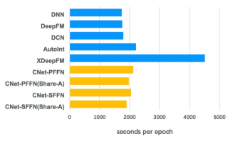
Figure 4. Efficiency comparison of different models in terms of run time per epoch on Criteo dataset

4.4. Ablation Study (RQ3)

In this section, we perform ablation experiments over key components of ContextNet in order to better understand their impacts on Criteo and Malware datasets(the other two datasets show similar trend), including linear contextual embedding (TCE), feed-forward network (FFN), layer normalization (LN), and residual connection (RC) . Table 4 shows the results of our default version (Block = $3$), and its variants on two datasets.

1. Remove TCE: The performance of ContextNet-PFFN dramatically degrades on both datasets without TCE module. It tells us that the contextual information gathered by TCE module is critical for the ContextNet and we deem TCE module extracts different high-order interactions information for various features.

2. Remove FFN: Without FFN, the model performance also degrades obviously and that may indicate the non-linear transformation on the result of element-wise product of feature embedding and contextual information is also important for ContextNet.

3. Remove LN or RC. From the results in Table 4, we can see that removing either LN or RC also decreases model performance, though the performance degradation is not as much as that of removing ICE and FFN.

We can see the usefulness of the different components of ContextNet from the above-mentioned ablation studies.

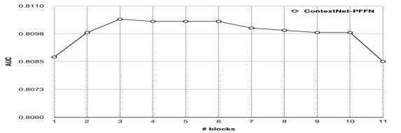
Figure 5. Effect of Different Blocks on Model Performance

4.5. Hyper-Parameter Study(RQ4)

In this section, we study the impact of hyper-parameters on ContextNet, including (1) the number of ContextNet blocks; (2) the number of feature embedding size. The experiments are conducted on Criteo and Malware datasets via changing one hyper-parameter while holding the other settings. Other two datasets show the similar trends and we didn’t present them because of the limited space.

Number of ContextNet Blocks.

To explore the influence of the number of ContextNet’s blocks on model’s performance, we conduct some experiments on Criteo dataset to stack blocks of ContextNet-PFFN model from $1$ block to $11$ blocks. Figure 5 shows the experimental results. It can be observe that the performance increases with more blocks at the beginning and the performance can be maintained until the number is set greater than $10$. Considering there are $4$ hidden layers in one block of Context-PFFN model, we can see that ContextNet-PFFN has the depth of nearly $40$ hidden layers in the model while keeping good performance. This may indicate that contextual embedding module helps the trainability of very deep network in CTR tasks.

Number of Feature Embedding Size.

The results in Table 5 show the impact of the number of feature embedding size on model performance. We can observe that the performance of ContextNet-PFFN increases with the increase of embedding size at the beginning. However, model performance degrades when the embedding size is set greater than $50$. Over-fitting of deep network is maybe the reason for this. Compared with the performance of the model shown in Table 2 which has a embedding size of $10$, the bigger embedding size further increases model’s performance on two datasets.

Table 5. Overall performance (AUC) of different feature embedding size of ContextNet-PFFN

	10	20	30	50	80
Criteo	0.8104	0.8109	0.8111	0.8113	0.8097
Malware	0.7399	0.7416	0.7417	0.7414	0.7405

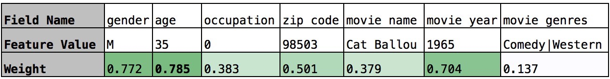
Figure 6. Example Instance from ML-1m

4.6. Analysis of Dynamic Feature Embedding (RQ5)

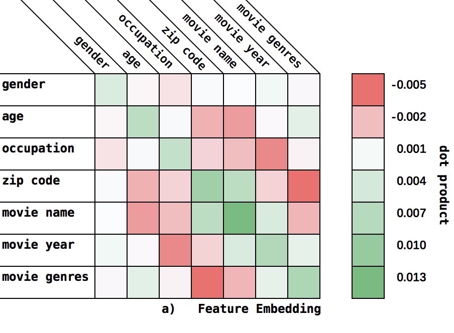
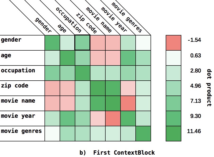
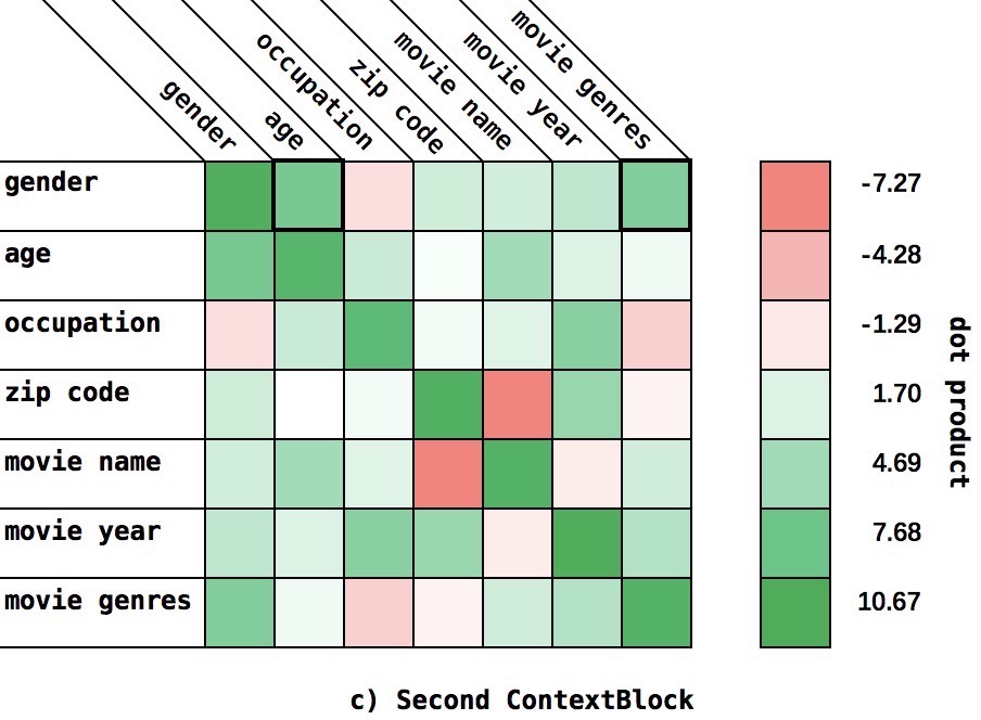
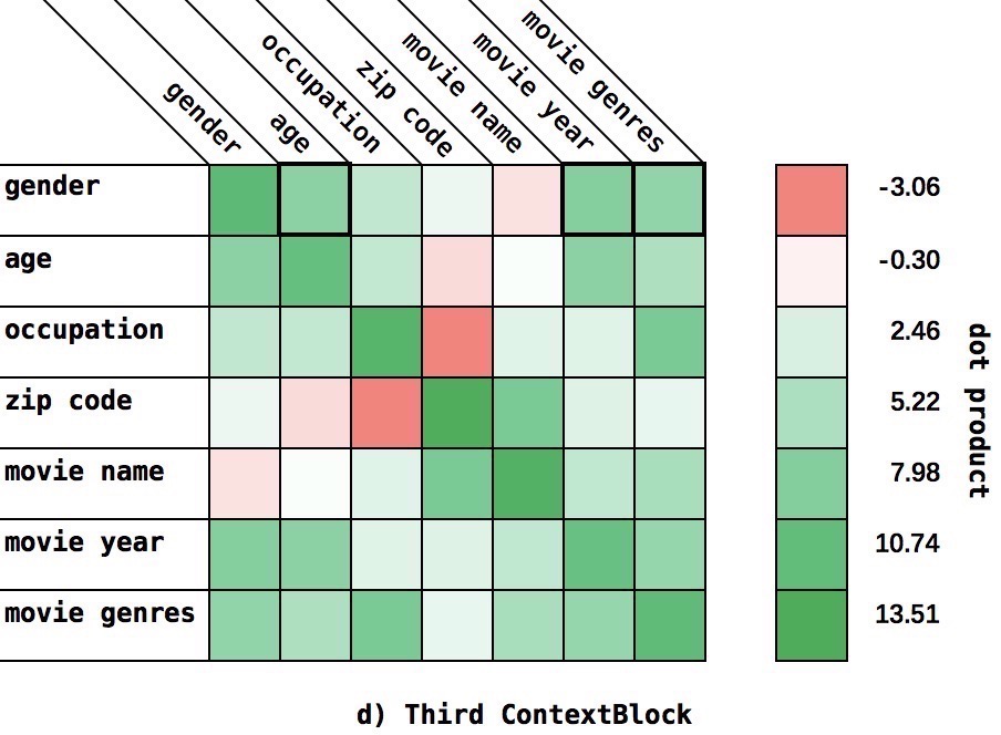
Figure 7. Analysis of Dynamic Feature Embedding

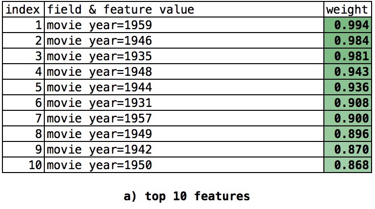
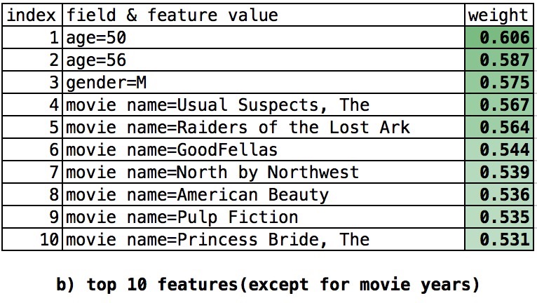
Figure 8. Top 10 Features of ML-1m Dataset

To verify that ContextNet indeed dynamically changes each feature’s embedding block by block to capture feature interactions, we input a randomly sampled instance (Figure 6, the instance has positive label with estimated CTR score $0.975$) from ML-1m dataset into trained ContextNet-PFFN. Then we compute the dot product for each feature pair using each ContextBlock’s outputted feature embedding, including the feature embedding layer. The high positive dot product value means the two feature have similar embedding content and are highly correlated interactions. The Figure 7 shows the result. The deeper green color means bigger positive value while deeper red color denotes bigger negative dot product value. The elements on the diagonal of the matrix can be ignored because that’s each feature’s self dot product. We can see from the Figure 7 that:

For features in feature embedding layer, most dot product values are small numbers near zero, which indicates the embedding values are very small and there is no correlation between different fields of input features. ( Fig. a of Figure 7). However, each feature’s embedding is dynamically changed by ContextBlock to gradually find the most useful feature interactions for its own purpose: more bigger dot product values begin to appear which means correlations between features. Take the field ”gender” as an example, if we adopt $5.0$ as the threshold, the highly correlated features change from ”occupation” ( Fig. b of Figure 7) to ”age” and ”movie genres” ( Fig. c of Figure 7). The final useful feature interactions focus on the features from field ”age”, ”movie year” and ”movie genres” ( Fig. d of Figure 7).

As for the feature importance analysis, we provide examples shown in Figure 6 and Figure 8. The feature contributes most to the final prediction score is ”age”=35 in this instance(Figure 6). Figure 8 shows the most important features in ML-1m dataset according to formula (16) in Section 3.6.

5. Conclusion

In this paper, We firstly propose a novel CTR Framework named ContextNet that implicitly models high-order feature interactions by dynamically refining the feature embedding. We also propose two specific models(ContextNet-PFFN and ContextNet-SFFN) under this framework. We conduct extensive experiments on four real-world datasets and the experiment results demonstrate that our proposed ContextNet-PFFN and ContextNet-SFFN model outperform state-of-the-art models such as DeepFM and xDeepFM significantly.

References

- (1)
- Ba et al. (2016) Jimmy Lei Ba, Jamie Ryan Kiros, and Geoffrey E Hinton. 2016. Layer normalization. arXiv preprint arXiv:1607.06450 (2016).
- Beutel et al. (2018a) A. Beutel, P. Covington, S. Jain, C. Xu, and E. H. Chi. 2018a. Latent Cross: Making Use of Context in Recurrent Recommender Systems. In the Eleventh ACM International Conference.
- Beutel et al. (2018b) Alex Beutel, Paul Covington, Sagar Jain, Can Xu, Jia Li, Vince Gatto, and Ed H Chi. 2018b. Latent cross: Making use of context in recurrent recommender systems. In Proceedings of the Eleventh ACM International Conference on Web Search and Data Mining. 46–54.
- Caruana (1993) Rich Caruana. 1993. Multitask Learning: A Knowledge-Based Source of Inductive Bias ICML. Google Scholar Google Scholar Digital Library Digital Library (1993).
- Caruana (1997) Rich Caruana. 1997. Multitask learning. Machine learning 28, 1 (1997), 41–75.
- Cheng et al. (2016) Heng-Tze Cheng, Levent Koc, Jeremiah Harmsen, Tal Shaked, Tushar Chandra, Hrishi Aradhye, Glen Anderson, Greg Corrado, Wei Chai, Mustafa Ispir, et al. 2016. Wide & deep learning for recommender systems. In Proceedings of the 1st workshop on deep learning for recommender systems. ACM, 7–10.
- Cho et al. (2014) Kyunghyun Cho, Bart Van Merriënboer, Caglar Gulcehre, Dzmitry Bahdanau, Fethi Bougares, Holger Schwenk, and Yoshua Bengio. 2014. Learning phrase representations using RNN encoder-decoder for statistical machine translation. arXiv preprint arXiv:1406.1078 (2014).
- Devlin et al. (2018) Jacob Devlin, Ming-Wei Chang, Kenton Lee, and Kristina Toutanova. 2018. Bert: Pre-training of deep bidirectional transformers for language understanding. arXiv preprint arXiv:1810.04805 (2018).
- Graepel et al. (2010) Thore Graepel, Joaquin Quinonero Candela, Thomas Borchert, and Ralf Herbrich. 2010. Web-scale bayesian click-through rate prediction for sponsored search advertising in microsoft’s bing search engine. Omnipress.
- Graves et al. (2013) Alex Graves, Abdel-rahman Mohamed, and Geoffrey Hinton. 2013. Speech recognition with deep recurrent neural networks. In 2013 IEEE international conference on acoustics, speech and signal processing. IEEE, 6645–6649.
- Guo et al. (2017) Huifeng Guo, Ruiming Tang, Yunming Ye, Zhenguo Li, and Xiuqiang He. 2017. DeepFM: a factorization-machine based neural network for CTR prediction. arXiv preprint arXiv:1703.04247 (2017).
- He et al. (2016) Kaiming He, Xiangyu Zhang, Shaoqing Ren, and Jian Sun. 2016. Deep residual learning for image recognition. In Proceedings of the IEEE conference on computer vision and pattern recognition. 770–778.
- He et al. (2014) Xinran He, Junfeng Pan, Ou Jin, Tianbing Xu, Bo Liu, Tao Xu, Yanxin Shi, Antoine Atallah, Ralf Herbrich, Stuart Bowers, et al. 2014. Practical lessons from predicting clicks on ads at facebook. In Proceedings of the Eighth International Workshop on Data Mining for Online Advertising. ACM, 1–9.
- Huang et al. (2019) Tongwen Huang, Zhiqi Zhang, and Junlin Zhang. 2019. FiBiNET: combining feature importance and bilinear feature interaction for click-through rate prediction. In Proceedings of the 13th ACM Conference on Recommender Systems. 169–177.
- Juan et al. (2016) Yuchin Juan, Yong Zhuang, Wei-Sheng Chin, and Chih-Jen Lin. 2016. Field-aware factorization machines for CTR prediction. In Proceedings of the 10th ACM Conference on Recommender Systems. ACM, 43–50.
- Koren et al. (2009) Yehuda Koren, Robert Bell, and Chris Volinsky. 2009. Matrix factorization techniques for recommender systems. Computer 8 (2009), 30–37.
- Krizhevsky et al. (2012) Alex Krizhevsky, Ilya Sutskever, and Geoffrey E Hinton. 2012. Imagenet classification with deep convolutional neural networks. In Advances in neural information processing systems. 1097–1105.
- Li et al. (2019) Z. Li, Z. Cui, S. Wu, X. Zhang, and L. Wang. 2019. Fi-GNN: Modeling Feature Interactions via Graph Neural Networks for CTR Prediction. (2019).
- Lian et al. (2018) Jianxun Lian, Xiaohuan Zhou, Fuzheng Zhang, Zhongxia Chen, Xing Xie, and Guangzhong Sun. 2018. xdeepfm: Combining explicit and implicit feature interactions for recommender systems. In Proceedings of the 24th ACM SIGKDD International Conference on Knowledge Discovery & Data Mining. ACM, 1754–1763.
- McMahan et al. (2013) H. Brendan McMahan, Gary Holt, D. Sculley, Michael Young, Dietmar Ebner, Julian Grady, Lan Nie, Todd Phillips, Eugene Davydov, Daniel Golovin, and et al. 2013. Ad Click Prediction: A View from the Trenches. In Proceedings of the 19th ACM SIGKDD International Conference on Knowledge Discovery and Data Mining (KDD ’13). Association for Computing Machinery, New York, NY, USA, 1222–1230. https://doi.org/10.1145/2487575.2488200
- Mikolov et al. (2013) Tomas Mikolov, Kai Chen, Greg Corrado, and Jeffrey Dean. 2013. Efficient estimation of word representations in vector space. arXiv preprint arXiv:1301.3781 (2013).
- Mikolov et al. (2010) Tomáš Mikolov, Martin Karafiát, Lukáš Burget, Jan Černockỳ, and Sanjeev Khudanpur. 2010. Recurrent neural network based language model. In Eleventh annual conference of the international speech communication association.
- Pennington et al. (2014) Jeffrey Pennington, Richard Socher, and Christopher D Manning. 2014. Glove: Global vectors for word representation. In Proceedings of the 2014 conference on empirical methods in natural language processing (EMNLP). 1532–1543.
- Peters et al. (2018) Matthew E Peters, Mark Neumann, Mohit Iyyer, Matt Gardner, Christopher Clark, Kenton Lee, and Luke Zettlemoyer. 2018. Deep contextualized word representations. arXiv preprint arXiv:1802.05365 (2018).
- Qu et al. (2016) Yanru Qu, Han Cai, Kan Ren, Weinan Zhang, Yong Yu, Ying Wen, and Jun Wang. 2016. Product-based neural networks for user response prediction. In 2016 IEEE 16th International Conference on Data Mining (ICDM). IEEE, 1149–1154.
- Radford et al. (2018) Alec Radford, Karthik Narasimhan, Tim Salimans, and Ilya Sutskever. 2018. Improving language understanding by generative pre-training.
- Rendle (2010) Steffen Rendle. 2010. Factorization machines. In 2010 IEEE International Conference on Data Mining. IEEE, 995–1000.
- Rendle et al. (2020) S. Rendle, W. Krichene, Z. Li, and J. Anderson. 2020. Neural Collaborative Filtering vs. Matrix Factorization Revisited. (2020).
- Song et al. (2019) Weiping Song, Chence Shi, Zhiping Xiao, Zhijian Duan, Yewen Xu, Ming Zhang, and Jian Tang. 2019. Autoint: Automatic feature interaction learning via self-attentive neural networks. In Proceedings of the 28th ACM International Conference on Information and Knowledge Management. 1161–1170.
- Tang et al. (2017) Hao Tang, Liang Lu, Lingpeng Kong, Kevin Gimpel, Karen Livescu, Chris Dyer, Noah A Smith, and Steve Renals. 2017. End-to-end neural segmental models for speech recognition. IEEE Journal of Selected Topics in Signal Processing 11, 8 (2017), 1254–1264.
- Vaswani et al. (2017) Ashish Vaswani, Noam Shazeer, Niki Parmar, Jakob Uszkoreit, Llion Jones, Aidan N Gomez, Lukasz Kaiser, and Illia Polosukhin. 2017. Attention is all you need. arXiv preprint arXiv:1706.03762 (2017).
- Wang et al. (2017) Ruoxi Wang, Bin Fu, Gang Fu, and Mingliang Wang. 2017. Deep & cross network for ad click predictions. In Proceedings of the ADKDD’17. ACM, 12.
- Xiao et al. (2017) Jun Xiao, Hao Ye, Xiangnan He, Hanwang Zhang, Fei Wu, and Tat-Seng Chua. 2017. Attentional factorization machines: Learning the weight of feature interactions via attention networks. arXiv preprint arXiv:1708.04617 (2017).
- Xie et al. (2020) Ruobing Xie, Cheng Ling, Yalong Wang, Rui Wang, Feng Xia, and Leyu Lin. 2020. Deep Feedback Network for Recommendation. 2491–2497. https://doi.org/10.24963/ijcai.2020/345
- Zhang et al. (2016) Weinan Zhang, Tianming Du, and Jun Wang. 2016. Deep learning over multi-field categorical data. In European conference on information retrieval. Springer, 45–57.
- Zhou et al. (2018) Guorui Zhou, Xiaoqiang Zhu, Chenru Song, Ying Fan, Han Zhu, Xiao Ma, Yanghui Yan, Junqi Jin, Han Li, and Kun Gai. 2018. Deep interest network for click-through rate prediction. In Proceedings of the 24th ACM SIGKDD International Conference on Knowledge Discovery & Data Mining. 1059–1068.