Leaf-FM: A Learnable Feature Generation Factorization Machine for Click-Through Rate Prediction

Abstract

Click-through rate (CTR) prediction is a fundamental task in personalized advertising and recommender systems. Though many models have been proposed such as FM, FFM and DeepFM in recent years, feature engineering is still a very important way to improve the model performance in many applications because using raw features can rarely lead to optimal results. For example, the continuous features are usually transformed to the power forms by adding a new feature to allow it to easily form non-linear functions of the feature. However, this kind of feature engineering heavily relies on peoples experience and it is both time consuming and labor consuming. In this paper, we propose LeafFM model based on FM to generate new features from the original feature embedding by learning the transformation functions automatically. We also design three concrete Leaf-FM models according to the different strategies of combing the original and the generated features. Extensive experiments are conducted on three real-world datasets and the results show Leaf-FM model outperforms standard FMs by a large margin. Compared with FFMs, Leaf-FM can achieve significantly better performance with much less parameters. In Avazu and Malware dataset, Leaf-FM can even achieve comparable performance with the DNN CTR models. As an improved FM model, Leaf-FM has the same computation complexity with FM in online serving phrase and it means Leaf-FM is applicable in many industry applications because of its better performance and high computation efficiency.

1 Introduction

CTR estimation is a fundamental task in personalized advertising and recommender systems. Many models have been proposed to resolve this problem such as Logistic Regression (LR) McMahan et al. (2013), tree-based models He et al. (2014), and Field-aware Factorization Machines (FFMs) Juan et al. (2016). In recent years, Some deep learning based models have been introduced and achieved success Zhang et al. (2016); Cheng et al. (2016); Guo et al. (2017); Lian et al. (2018); Qu et al. (2016).

However, feature engineering is still a very important way to improve the model performance in these systems because using raw features can rarely lead to optimal results. In order to generate better performance models, usually a lot of work on the transformation of raw features is needed. For example, proper normalization of continuous features was critical for model convergence and the continuous features are usually transformed to the power forms by adding a new feature to allow it to easily form non-linear or sub-linear functions of the featureCovington et al. (2016). Say, in addition to the raw normalized feature $x$, we also input powers $x^{2}$ and $\sqrt{x}$ as new features into model. However, this kind of feature engineering heavily relies on people’s experience and it is both time consuming and labor consuming. In order to promote the model’s expressive ability and reduce the engineering resources, it’s necessary to make these feature generation work to be automatic.

In this work, we propose Leaf-FM model based on FMs to generate new features from the original feature embedding by learning the transformation functions automatically, which greatly enhances the expressive ability of model and saves the cost of feature engineering.

The contributions of our work are summarized as follows:

1. We propose a novel Feature Generation Network (FGNet) to learn to automatically generate new features from the original one during model training, including both the continuous feature and categorical features. FGNet can greatly reduce the need for feature engineering in many real-world CTR tasks.

2. We propose a new model named LEArnable Feature-generation Factorization Machine(Leaf-FM) which uses FGNet to boost the FM model’s performance. We design three specific Leaf-FM models according to the different strategies of combing the original and the generated features: add version(LA-FM), sum version(LS-FM) and product version(LP-FM). The experiments show that the automatically generated features indeed boost the FM model’s performance significantly.

3. We conduct extensive experiments on three real-world datasets and the experiment results show that Leaf-FM model outperforms standard FMs by a large margin. Compared with FFMs, Leaf-FM can achieve significantly better performance with much less parameters. On Avazu and Malware datasets, Leaf-FM can even achieve comparable performance with the DNN and DeepFM models.

4. As an improved FM model, Leaf-FM has the same computation complexity with FM in online serving phrase and it means Leaf-FM is applicable in many industry applications because of its better performance and high computation efficiency.

The rest of this paper is organized as follows. Section 2 introduces some related works which are relevant with our proposed model. Some preliminaries are described in Section 3 for easy understanding of the proposed model. We introduce our proposed Leaf-FM model in detail in Section 4. The experimental results on Criteo and Avazu datasets are presented and discussed in Section 5. Section 6 concludes our work in this paper.

2 Related Work

Factorization Machines (FMs) Rendle (2010) and Field-aware Factorization Machines (FFMs) Juan et al. (2016) are two of the most successful CTR models. Other linear FM-based models are proposed, such as CoFM Hong et al. (2013), FwFM Pan et al. (2018) and importance-aware FM Oentaryo et al. (2014). However, these models show limited effectiveness in mining high-order latent patterns or learning quality feature representations.

Another line of research on FM-based models is to incorporate deep neural networks (DNNs). For example, Factorization-Machine Supported Neural Networks (FNN)Zhang et al. (2016), as well as the product-based neural network (PNN)Qu et al. (2016), are feed-forward neural networks using FM to pre-train the embedding layer. More recently, hybrid architectures are introduced in Wide&Deep Cheng et al. (2016), DeepFM Guo et al. (2017) and xDeepFM Lian et al. (2018) by combining shallow components with deep ones to capture both low- and high-order feature interactions. However, some DNN models significantly increase the computation time and it’s hard to deploy it in real-world applications.

3 Preliminaries

3.1 Factorization Machines and Field-aware Factorization Machine

Factorization Machines (FMs) Rendle (2010) is one of the most widely used CTR models in many real-world applications because of its conciseness.

As we all know, FMs model interactions between features $i$ and $j$ as the dot products of their corresponding embedding vectors as follows:

$$\hat{y}(x)=w_{0}+\sum^{m}_{i=1}w_{i}x_{i}+\sum^{m}_{i=1}\sum^{m}_{j=i+1}\left<v_{i},v_{j}\right>x_{i}x_{j}$$ (1)

An embedding vector $v_{i}\in\mathbb{R}^{d}$ for each feature is learned by FM, $d$ is a hyper-parameter which is usually a small integer and $m$ is the feature number. However, FM neglects the fact that a feature might behave differently when it interacts with features from other fields. To explicitly take this difference into consideration, Field-aware Factorization Machines (FFMs) learn extra $f-1$ embedding vectors for each feature(here $f$ denotes field number):

$$\hat{y}(x)=w_{0}+\sum^{m}_{i=1}w_{i}x_{i}+\sum^{m}_{i=1}\sum^{m}_{j=i+1}\left<v_{ij},v_{ji}\right>x_{i}x_{j}$$ (2)

where $v_{ij}\in\mathbb{R}^{d}$ denotes the embedding vector of the $j$-th entry of feature $i$ when feature $i$ is interacting with fields $j$. $d$ is the embedding size.

3.2 Layer Normalization

Normalization techniques have been recognized as very effective components in deep learning. For example, Batch Normalization (Batch Norm or BN)Ioffe and Szegedy (2015) normalizes the features by the mean and variance computed within a mini-batch. This has been shown by many practices to ease optimization and enable very deep networks to converge. Another example is layer normalization (Layer Norm or LN)Ba et al. (2016) which was proposed to ease optimization of recurrent neural networks. Statistics of layer normalization are not computed across the $N$ samples in a mini-batch but are estimated in a layer-wise manner for each sample independently. Specifically, assuming the input is a vector $\mathbf{x}$ which contains all features of a sample, the operation is defined as:

$$\mathbf{LayerNorm}(\mathbf{x})=\mathbf{\alpha}\odot\frac{\mathbf{x}-\mu}{\delta^{2}+\epsilon}+\mathbf{\beta}$$ (3)

where $\odot$ is an element-wise product (i.e., the Hadamard product), $\mu$ and $\delta$ are the mean and variance of $\mathbf{x}$, $\mathbf{\alpha}$ and $\mathbf{\beta}$ are learned scaling factors and bias terms.

4 Our Proposed Model

As mentioned in the section 1, feature engineering such as transforming the input continuous features to the sub-linear or super-linear form helps promote the model performance. However, the experience about how to transform the continuous feature needs expert knowledge. In real-world applications, considerable user’s demographics and item’s attributes are usually categorical. It seems hard to adopt the similar feature transformation on categorical feature.

In this paper, we intent to automatically learn the transformed new feature from the original one and boost FM model’s expressive ability by combing those new generated feature. We learn the generated new feature through a network on the feature embedding.

As all we know, features in CTR tasks usually can be segregated into the following two groups.

1. categorical features. This type of feature is common and the one-hot representation may produce very sparse features. We usually map one-hot representation to dense, low-dimensional embedding vectors suitable for complex transformation and these embedding carry richer information than one-hot representations.

2. Numerical features. There are two widely used approaches to convert the numerical feature into embedding. The first one is to quantize each numerical feature into discrete buckets, and the feature is then represented by the bucket ID. We can map bucket ID to an embedding vector. The second method maps the feature field into an embedding vector as follows:

   $$v_{i}=e_{i}x_{i}$$ (4)

   where $e_{i}$ is an embedding vector for field $i$, and $x_{i}$ is a scalar value. In our experiments, we adopt the second approach to convert numerical features into embedding.

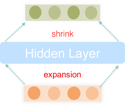
Figure 1: Structure of Feature Generation Network

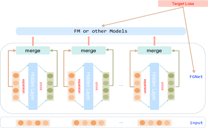
Figure 2: Structure of Leaf-FM

4.1 Learn to Generate New Feature

In order to enhance the model’s expressive ability by learning to generate new features from the original one, we propose a Feature Generation Network(FGNet) in this work as depicted in Figure 1.

Suppose a feature $v_{i}$ is one feature in field $k$ . To generate the new feature from $v_{i}$, two fully connected (FC) layers are used on feature $v_{i}$. The first FC layer is a dimensionality-expansion layer with parameters $W_{k1}$ and expansion ratio $r$ which means the size of FC layer is $rd$ if the vector size is $d$ and it is a hyper-parameter. The second FC layer decreases dimensionality with parameters $W_{k2}$, which is equal to dimension of feature embedding $v_{i}$. Formally, the feature generation process is calculated as follows:

$$g_{i}=\mathcal{F}_{FGNet}(v_{i},W_{k})=\delta(W_{k2}\cdot\delta(W_{k1}\cdot v_{i}))$$ (5)

where $\delta$ refers to the non-linear function, $W_{k1}\in\mathbb{R}^{d\times rd}$ and $W_{k2}\in\mathbb{R}^{rd\times d}$. The size of generated feature $g_{i}$ is $d$, which is equal to the size of original embedding. Notice here that each feature field maintains its parameters $W_{k}$ and the total number of parameters for feature generation is $f\ast W_{k}$. $f$ is the number of fields.

Though the above-mentioned feature generation module has only two FC layers, we can stack FC layers to add further non-linear transformation for each original feature vector $v_{i}$ in order to generate better new features. So the depth of feature generation module can be regarded as a hyper-parameter.

In this way, this network can be trained to learn to transform original feature to a super-linear or sub-linear form, which can be added into models as new features. Notice that it’s a general approach to learn to generate new feature and doesn’t relies on concrete model we used.

4.2 Leaf-FM

In this paper, we propose Leaf-FM model as depicted in Figure 2 to show how to combine this feature generation module and FM models to improve the baseline model’s performance. As mentioned above, we can learn to generate one or more new transformed features $g_{i}$ for each feature $v_{i}$ and there are various merging strategies to combine the original feature and generated features during model training in the FM models. We propose three version of Leaf-FM according to the different feature merging methods in this work.

Suppose we use the FGNet generate some new features for each feature $v_{i}$, we have the following feature set for $v_{i}$:

$$FS_{v_{i}}=\left\{v_{i},g_{i1},...,g_{ij},...,g_{iu}\right\}$$ (6)

where $g_{ij}$ is the $j$-th generated feature from feature $v_{i}$, $u$ is the number of new generated features for each feature $v_{i}$.

4.2.1 Add Version Leaf-FM

A direct method to merge the newly generated features in FM is to regard these features as independent new features and directly add them into the model. So the feature numbers of FM increase from m to $(u+1)m$ if we generate $u$ new feature for each feature $v_{i}$. We call this version Leaf-FM ’Add version Leaf-FM’(LA-FM) which has the following format:

$$\hat{y}(x)=w_{0}+\sum^{m}_{i=1}w_{i}x_{i}+\sum^{(u+1)m}_{i=1}\sum^{(u+1)m}_{j=i+1}\left<v_{i},v_{j}\right>x_{i}x_{j}$$ (7)

For this version Leaf-FM, we use either Relu or identity as non-linear function($\Phi(x)$) in feature generation network:

$$g_{i}=\mathcal{F}_{FGNet}(v_{i},W_{k},\beta_{k})=\Phi(W_{k2}\Phi(W_{k1}v_{i}+\mathbf{\beta}_{k1})+\mathbf{\beta}_{k2})$$ (8)

4.2.2 Sum Version Leaf-FM

Another merging approach is to sum all the features in feature set $FS_{vi}$ to one vector as follows:

$$\mathcal{F}_{s}(v_{i})=v_{i}+\sum_{j=1}^{u}g_{ij}$$ (9)

where $\mathcal{F}_{s}(v_{i})$ is the merged new feature vector which is equal to the size of feature $v_{i}$, $g_{ij}$ is the $j$-th generated feature from feature $v_{i}$, $u$ is the number of new generated features for each feature $v_{i}$. We call Leaf-FM with this kind of merging strategy ’Sum Version Leaf-FM’(LS-FM) and LS-FM model has the following format:

$$\hat{y}(x)=w_{0}+\sum^{m}_{i=1}w_{i}x_{i}+\sum^{m}_{i=1}\sum^{m}_{j=i+1}\left<\mathcal{F}_{s}(v_{i}),\mathcal{F}_{s}(v_{j})\right>x_{i}x_{j}$$ (10)

For this version Leaf-FM, we also use Relu as non-linear function in feature generation network:

$$g_{i}=\mathcal{F}_{FGNet}(v_{i},W_{k},\beta_{k})=Relu(W_{k2}Relu(W_{k1}v_{i}+\beta_{k1})+\beta_{k2})$$ (11)

4.2.3 Product Version Leaf-FM

In order to increase the non-linearity of the merging process, we can merge the new generated feature $g_{i}$ and original feature $v_{i}$ by element-product and normalization as follows:

$$\mathcal{F}_{p}(v_{i})=LayerNorm(g_{i}\otimes v_{i})$$ (12)

where $g_{i}$ is the generated feature from feature $v_{i}$, $\otimes$ is the element-wise product of two vectors, the layer normalization is used on the results of element-wise product to further increase the non-linear ability of the generating model.

We call Leaf-FM with this merging strategy ’Product Version Leaf-FM’(LP-FM) and LP-FM model has the following format:

$$\hat{y}(x)=w_{0}+\sum^{m}_{i=1}w_{i}x_{i}+\sum^{m}_{i=1}\sum^{m}_{j=i+1}\left<\mathcal{F}_{p}(v_{i}),\mathcal{F}_{p}(v_{j})\right>x_{i}x_{j}$$ (13)

For this version Leaf-FM, we use identity function in feature generation network:

$$g_{i}=\mathcal{F}_{\tiny{FGNet}}(v_{i},W_{k},\beta_{k})=W_{k2}(W_{k1}v_{i}+\beta_{k1})+\beta_{k2}$$ (14)

4.3 Joint Training of Feature Generation Module and FM

Since the Leaf-FM has two parts of parameters to train: feature vectors in FM and the FC network parameters in feature generation module, so we can train them jointly.

For binary classifications, the loss function is the log loss:

$$\mathcal{L}=-\frac{1}{N}\sum^{N}_{i=1}y_{i}\log(\hat{y}_{i})+(1-y_{i})\log(1-\hat{y}_{i})$$ (15)

where $N$ is the total number of training instances, $y_{i}$ is the ground truth of $i$-th instance and $\hat{y}_{i}$ is the predicted CTR. The optimization process is to minimize the following objective function:

$$\mathfrak{L}=\mathcal{L}+\lambda\|\Theta\|$$ (16)

where $\lambda$ denotes the regularization term and $\Theta$ denotes the set of parameters, including these in feature vector matrix and feature generation module.

Table 1: A summary of model complexities (ignoring the bias term) and computation efficiency. m and f are feature number and field number respectively, d is the embedding vector dimension, and r is the reduction ratio of FC for Leaf-FM models.

	Number of	Offline	Online
Models	parameters	Training	Serving
FM	$m+m\ast d$	$O(m\ast d)$	$O(m\ast d)$
FFM	$m+m\ast(f-1)\ast d$	$O(m^{2}\ast d)$	$O(m^{2}\ast d)$
Leaf-FM	$m+m\ast d+f\ast 2(rd\ast d)$	$O(m^{2}\ast d)$	$O(m\ast d)$

4.4 Model Complexity and Computation Efficiency

FM is widely used in many industry applications because of its high computation efficiency. As shown in Table 1, the number of parameters in FM is $m+m\ast d$, where $m$ accounts for the weights for each feature in the linear part $\{w_{i}|i=1,...,m\}$ and $m\ast d$ accounts for the embedding vectors for all the features $\{v_{i}|i=1,...,m\}$. FM has a $O(m\ast d)$ linear runtime, which makes it applicable from a computational point of view.

In recent years, many new models such as FFM and DeepFM have been proposed. Though the performances are boosted greatly , many new models’s high model complexity hinders their real-word application. For example, the number of parameters of FFM is $m+m\ast(f$ - 1$)\ast d$ since each feature has $f$ - $1$ embedding vectors and it has a $O(m^{2}\ast d)$ computation complexity.

Leaf-FM use $f\ast 2(rd\ast d)$ additional parameters for generating new features so that the total number of parameters of Leaf-FM is $m+m\ast d+f\ast 2(rd\ast d)$ . So the parameter number of Leaf-FM is comparable with that of FM and significantly less than that of FFM. Though the offline training of Leaf-FM needs $O(m^{2}\ast k)$ runtime in order to jointly train the feature generation module, Leaf-FM has the same computation complexity with FM in online serving phrase. After training the Leaf-FM, we can transform the original feature $v_{i}$ to $F_{s}(v_{i})$ for each feature in offline phrase . So the standard FM can be used in online serving phrase and that means our proposed Leaf-FM model is applicable in industry applications because of its better model’s performance and high computation efficiency.

5 Experimental Results

To comprehensively evaluate our proposed method, we design some experiments to answer the following research questions:

• RQ1 Are the new features generated by Feature Generation Network useful for FM model? How does the number of the newly generated features influence the model performance?

• RQ2 Can our proposed several Leaf-FM models outperform complex models like FFM? How about the performance comparison even with the deep learning based models such as DNN and DeepFM?

• RQ3 How does the hyper-parameters of Feature Generation Network influence the model performance?

• RQ4 How does the hyper-parameters of Leaf-FM influence the model performance?

In the following, we will first describe the experimental settings, followed by answering the above research questions.

5.1 Experiment Setup

Datasets

The following three data sets are used in our experiments:

1. Criteo Dataset: As a very famous public real world display ad dataset with each ad display information and corresponding user click feedback, Criteo data set is widely used in many CTR model evaluation. There are 26 anonymous categorical fields and 13 continuous feature fields in Criteo data set.

2. Avazu Dataset: The Avazu dataset consists of several days of ad click- through data which is ordered chronologically. For each click data, there are 24 fields which indicate elements of a single ad impression.

3. Malware Dataset: Malware is a dataset from Kaggle competitions published in the Microsoft Malware Classification Challenge. It is almost half a terabyte when uncompressed and consists of disassembly and bytecode malware files representing a mix of 9 different families.

We randomly split instances by 8:1:1 for training , validation and test while Table 2 lists the statistics of the evaluation datasets. For these datasets, a small improvement in prediction accuracy is regarded as practically significant because it will bring a large increase in a company’s revenue if the company has a very large user base.

Table 2: Statistics of the evaluation datasets

Datasets	#Instances	#fields	#features
Criteo	45M	39	30M
Avazu	40.43M	24	0.64M
Malware	8.92M	82	9.89M

Evaluation Metrics

AUC (Area Under ROC) is used in our experiments as the evaluation metrics. This metric is very popular for binary classification tasks. AUC’s upper bound is 1 and larger value indicates a better performance.

Models for Comparisons

We compare the performance of the FM, FFM, DNN and DeepFM models as baseline and all of which are discussed in Section 2 and Section 3.

Implementation Details

We implement all the models with Tensorflow in our experiments. For optimization method, we use the Adam with a mini-batch size of $1000$ and a learning rate is set to $0.0001$. We make the dimension of field embedding for all models to be a fixed value of $10$ for FM-related models and $4$ for FFM model. For models with DNN part, the depth of hidden layers is set to $3$, the number of neurons per layer is $400$, all activation function are ReLU and dropout rate is set to $0.5$. We conduct our experiments with $2$ Tesla $K40$ GPUs.

5.2 Usefulness of the Generated Features(RQ1)

The overall performance for CTR prediction of different models on three real-world datasets is shown in Table 3. Compared with the performance of FM model, the three versions of Leaf-FM outperform FM by a large margin almost on all datasets. Because the only difference between the FM and Leaf-FM model is that Leaf-FM uses the new features generated by feature generation network, we can draw the conclusion that the generated features by FGNet can greatly increase the simple model’s expressive ability by automatically learning to add some transformed sub-linear and super-linear new features. The only exception is the performance of product version Leaf-FM model on Malware dataset and this indicates how to merge the original features and generated features still matters on different dataset.

Table 3: Overall performance (AUC) of different models on three datasets(d=4 for FFM and 10 for all other model, $d$ means embedding size, $l$ means depth of DNN, $n$ means the size of FC layer of DNN, $p$ means network depth of FGNet, $g$ means number of the generated feature; $e$ means expansion rate)

Model	Setting	Criteo	Malware	Avazu
FM	$d$=10	0.7896	0.7225	0.7757
FFM	$d$=4	0.7951	0.7240	0.7791
DNN	$l$=3;$n$=400	0.8054	0.7263	0.7820
DeepFM	$l$=3;$n$=400	0.8056	0.7295	0.7833
LA-FM	$e$=1;$p$=2;$g$=3	0.7956	0.7281	0.7819
LS-FM	$e$=1;$p$=2;$g$=3	0.8003	0.7260	0.7803
LP-FM	$e$=1;$p$=2;$g$=1	0.8005	0.7167	0.7803

We conduct some experiments to observe the influence of the number of newly generated features for each original feature on LA-FM model on Cretio dataset. The experimental results are shown in Table 4. From the results, we can see that the performance increases gradually with the increase of the number of newly generated features until the number reaches 11. This indicates that the more features generated by the FGNet, the more useful information we can get.

Table 4: Overall performance (AUC) of Add version LeafFM with different number of newly generated features for each original feature on Criteo dataset(embedding size=10,network depth=2,expansion rate=1)

	1	3	5	7	9	11
LA-FM	0.7993	0.8003	0.8008	0.8013	0.8015	0.8019

5.3 Performance Comparison(RQ2)

From the experimental results shown in Table 3, we have the following key observations:

1. Leaf-FM significantly outperforms more complex models like FFM on almost all three datasets. Considering Leaf-FM has much less parameters and nearly linear online runtime, we can see that Leaf-FM model is a much more applicable CTR model.

2. Compared even with deep learning based CTR models such as DNN and DeepFM models, add version Leaf-FM (LA-FM) can achieve comparable performance on Malware and Avazu datasets. LA-FM even outperforms DNN model on Malware dataset and that’s out of our expectation. Because DNN model use MLP to capture high-order feature interaction and FM-like model doesn’t has this ability. This may suggests that some feature engineering work like feature transformation is important for some dataset such as Malware and Avazu. The experimental results also prove that Leaf-FM model works well by automatically learning to generate new features and it can be used to reduce the human labor in feature engineering in many real-world CTR tasks.

3. As for the comparison of three different versions of Leaf-FM, we can see from the results that feature merging approach still matters. Different tasks need specific feature merging strategy. For example, LS-FM and LP-FM outperform LA-FM on Cretio dataset while LA-FM and LS-FM are better choices for Malware dataset.

4. As an improved FM model, Leaf-FM has the same computation complexity with FM in online serving phrase . At the same time, Leaf-FM has comparable performance with some DNN models. These mean Leaf-FM is applicable in many industry applications because of its better performance and high computation efficiency.

Table 5: Overall performance (AUC) of Add version LeafFM with different expansion rate on Criteo dataset(embedding size=10,network depth=2,number of the generated feature=1)

	1	2	3	4	5	7
LA-FM	0.7993	0.7994	0.7996	0.8002	0.7980	0.7990

5.4 Hyper-Parameter of FGNet(RQ3)

In this section, we study the impact of hyper-parameters of Feature Generation Network on Leaf-FM model. For the FG network, expansion rate and network depth are two hyper-parameters to influence the model performance. The experiments are conducted on Criteo datasets via changing one hyper-parameter while holding the other settings.

Expansion Rate.

We conduct some experiments to adjust the expansion rate in LA-FM model from 1 to 7,which means size of hidden layer is from 10 to 70 because the embedding size is set 10. We list the results in Table 5. We can observe a slightly performance increase with the increase of expansion rate until it’s greater than 4.

Table 6: Overall performance (AUC) of Add version LeafFM with different network depth on Criteo dataset(embedding size=10,expansion rate=1, number of the generated feature=1))

	2	3	4	5	7	10
LA-FM	0.7993	0.7991	0.7996	0.8003	0.8001	0.7946

Depth of Network.

The results in Table 6 show the impact of number of hidden layers. We can observe that the performance of LA-FM increases with the depth of network at the beginning. However, model performance degrades when the depth of network is set greater than 5. Over-fitting of deep network is maybe the reason for this.

5.5 Hyper-Parameter of Leaf-FM (RQ4)

In this section, we study the impact of hyper-parameters on Leaf-FM model. For the FM or FFM models, the number of feature embedding size is our main concern. The experiments are conducted on Criteo datasets via changing embedding size from 10 to 120 while holding the other settings.

Embedding Size.

Table 7 shows the experimental results . It can be seen that the number of feature embedding size greatly influences the model performance. With the increase of this number, the performance increases rapidly until the number reaches 100. The AUC of the model with embedding size 100 is 0.8055,which outperforms the DNN model with the same embedding size.

Table 7: Overall performance (AUC) of Add version LeafFM with different embedding size on Criteo dataset(expansion rate=1,network depth=2,number of the generated feature=1)

	10	30	50	80	100	120
LA-FM	0.7993	0.8030	0.8048	0.8054	0.8055	0.8051

6 Conclusion

In this paper, we propose Leaf-FM model to generate new features from the original feature embedding by learning the transformation functions automatically, which greatly enhances the expressive ability of model and saves the cost of feature engineering. Extensive experiments are conducted on real-world datasets and the results show Leaf- FM model outperforms standard FMs by a large margin. Leaf-FM even can achieve comparable performance with the DNN CTR models. As an improved FM model, Leaf-FM has the same computation complexity with FM in online serving phrase and it means Leaf-FM is applicable in many industry applications because of its better model’s performance and high computation efficiency.

References

- Ba et al. [2016] Jimmy Lei Ba, Jamie Ryan Kiros, and Geoffrey E Hinton. Layer normalization. arXiv preprint arXiv:1607.06450, 2016.
- Cheng et al. [2016] Heng-Tze Cheng, Levent Koc, Jeremiah Harmsen, Tal Shaked, Tushar Chandra, Hrishi Aradhye, Glen Anderson, Greg Corrado, Wei Chai, Mustafa Ispir, et al. Wide & deep learning for recommender systems. In Proceedings of the 1st workshop on deep learning for recommender systems, pages 7–10. ACM, 2016.
- Covington et al. [2016] Paul Covington, Jay Adams, and Emre Sargin. Deep neural networks for youtube recommendations. In Proceedings of the 10th ACM conference on recommender systems, pages 191–198. ACM, 2016.
- Guo et al. [2017] Huifeng Guo, Ruiming Tang, Yunming Ye, Zhenguo Li, and Xiuqiang He. Deepfm: a factorization-machine based neural network for ctr prediction. arXiv preprint arXiv:1703.04247, 2017.
- He et al. [2014] Xinran He, Junfeng Pan, Ou Jin, Tianbing Xu, Bo Liu, Tao Xu, Yanxin Shi, Antoine Atallah, Ralf Herbrich, Stuart Bowers, et al. Practical lessons from predicting clicks on ads at facebook. In Proceedings of the Eighth International Workshop on Data Mining for Online Advertising, pages 1–9. ACM, 2014.
- Hong et al. [2013] Liangjie Hong, Aziz S Doumith, and Brian D Davison. Co-factorization machines: modeling user interests and predicting individual decisions in twitter. In Proceedings of the sixth ACM international conference on Web search and data mining, pages 557–566. ACM, 2013.
- Ioffe and Szegedy [2015] Sergey Ioffe and Christian Szegedy. Batch normalization: Accelerating deep network training by reducing internal covariate shift. arXiv preprint arXiv:1502.03167, 2015.
- Juan et al. [2016] Yuchin Juan, Yong Zhuang, Wei-Sheng Chin, and Chih-Jen Lin. Field-aware factorization machines for ctr prediction. In Proceedings of the 10th ACM Conference on Recommender Systems, pages 43–50. ACM, 2016.
- Lian et al. [2018] Jianxun Lian, Xiaohuan Zhou, Fuzheng Zhang, Zhongxia Chen, Xing Xie, and Guangzhong Sun. xdeepfm: Combining explicit and implicit feature interactions for recommender systems. In Proceedings of the 24th ACM SIGKDD International Conference on Knowledge Discovery & Data Mining, pages 1754–1763. ACM, 2018.
- McMahan et al. [2013] H. Brendan McMahan, Gary Holt, D. Sculley, Michael Young, Dietmar Ebner, Julian Grady, Lan Nie, Todd Phillips, Eugene Davydov, Daniel Golovin, and et al. Ad click prediction: A view from the trenches. In Proceedings of the 19th ACM SIGKDD International Conference on Knowledge Discovery and Data Mining, KDD ’13, page 1222–1230, New York, NY, USA, 2013. Association for Computing Machinery.
- Oentaryo et al. [2014] Richard J Oentaryo, Ee-Peng Lim, Jia-Wei Low, David Lo, and Michael Finegold. Predicting response in mobile advertising with hierarchical importance-aware factorization machine. In Proceedings of the 7th ACM international conference on Web search and data mining, pages 123–132. ACM, 2014.
- Pan et al. [2018] Junwei Pan, Jian Xu, Alfonso Lobos Ruiz, Wenliang Zhao, Shengjun Pan, Yu Sun, and Quan Lu. Field-weighted factorization machines for click-through rate prediction in display advertising. In Proceedings of the 2018 World Wide Web Conference, pages 1349–1357. International World Wide Web Conferences Steering Committee, 2018.
- Qu et al. [2016] Yanru Qu, Han Cai, Kan Ren, Weinan Zhang, Yong Yu, Ying Wen, and Jun Wang. Product-based neural networks for user response prediction. In 2016 IEEE 16th International Conference on Data Mining (ICDM), pages 1149–1154. IEEE, 2016.
- Rendle [2010] Steffen Rendle. Factorization machines. In 2010 IEEE International Conference on Data Mining, pages 995–1000. IEEE, 2010.
- Zhang et al. [2016] Weinan Zhang, Tianming Du, and Jun Wang. Deep learning over multi-field categorical data. In European conference on information retrieval, pages 45–57. Springer, 2016.