ThunderRW: An In-Memory Graph Random Walk Engine

Abstract.

As random walk is a powerful tool in many graph processing, mining and learning applications, this paper proposes an efficient in-memory random walk engine named ThunderRW. Compared with existing parallel systems on improving the performance of a single graph operation, ThunderRW supports massive parallel random walks. The core design of ThunderRW is motivated by our profiling results: common RW algorithms have as high as 73.1% CPU pipeline slots stalled due to irregular memory access, which suffers significantly more memory stalls than the conventional graph workloads such as BFS and SSSP. To improve the memory efficiency, we first design a generic step-centric programming model named Gather-Move-Update to abstract different RW algorithms. Based on the programming model, we develop the step interleaving technique to hide memory access latency by switching the executions of different random walk queries. In our experiments, we use four representative RW algorithms including PPR, DeepWalk, Node2Vec and MetaPath to demonstrate the efficiency and programming flexibility of ThunderRW. Experimental results show that ThunderRW outperforms state-of-the-art approaches by an order of magnitude, and the step interleaving technique significantly reduces the CPU pipeline stall from 73.1% to 15.0%.

1. Introduction

Random walk (RW) is an effective tool for extracting relationships between entities in a graph, and is widely used in many applications such as Personalized PageRank (PPR) (Page et al., 1999), SimRank (Jeh and Widom, 2002), Random Walk Domination (Li et al., 2014), Graphlet Concentration (GC) (Pržulj, 2007), Network Community Profiling (NCP) (Fortunato and Hric, 2016), DeepWalk (Perozzi et al., 2014) and Node2Vec (Grover and Leskovec, 2016). For graph analysis tasks such as GC and NCP, RW queries generally dominate the cost (Pržulj, 2007; Fortunato and Hric, 2016). Even for graph representation learning, the cost of sampling RW is non-trivial, for example, a naive implementation of Node2Vec takes more than eight hours on the twitter graph in our experiments. Moreover, increasing the number of RW queries can improve the effectiveness of RW algorithms (Grover and Leskovec, 2016; Pržulj, 2007). Therefore, accelerating RW queries is an important problem.

RW algorithms generally follow the execution paradigm illustrated in Algorithm 1, which consists of massive RW queries. Each query $Q$ starts from a given source vertex. At each step, $Q$ moves to a neighbour of the current residing vertex at random, and repeats this process until satisfying a specific termination condition, e.g., a target length is reached (Lines 2-5). Despite that RW algorithms follow a similar execution paradigm, there are quite some variants of RW algorithms, which can differ significantly in neighbor selections (see Section 2.2). Encouraged by the success of in-memory graph processing engines (Shun and Blelloch, 2013; Nguyen et al., 2013; Zhang et al., 2018; Sundaram et al., 2015), there have been some recent systems designed specifically for RW algorithms, including C-SAW (Pandey et al., [n.d.]), GraphWalker (Wang et al., 2020) and KnightKing (Yang et al., 2019). They focus on accelerators, disk-based or distributed settings, without specially optimizing in-memory execution of RW queries. However, with the rapid development of hardwares, modern servers equip with hundred gigabytes, even several terabytes memory, which empowers in-memory processing of graphs with hundred billions of edges. This covers many real-world graphs in applications (Dhulipala, [n.d.]). As such, this paper studies the design and implementation of an in-memory graph engine for RW algorithms.

Input: a graph $G$ and a set $\mathbb{Q}$ of random walk queries;

Output: the walk sequences of each query in $\mathbb{Q}$;

1 foreach $Q\in\mathbb{Q}$ do

2       do

3             Select a neighbor of the current residing vertex $Q.cur$ at random;

4             Add the selected vertex to $Q$;

5            

6      while Terminate($Q$) is false;

7return $\mathbb{Q}$;

Algorithm 1 Execution Paradigm of RW algorithms

To crystallize the performance factors for in-memory RW executions, we conduct profiling studies on RW algorithms in comparison with conventional workloads of a single graph operation like BFS and SSSP (see Section 3). Our profiling results show that common RW algorithms have as high as 73.1% CPU pipeline slots stalled due to irregular memory access, which suffers significantly more memory stalls than the conventional workloads. Consequently, the CPUs frequently wait on the high-latency access to the main memory, which becomes the major performance bottleneck. Besides, we observe that the sampling methods such as inverse transformation sampling (Marsaglia, 1963), alias sampling (Walker, 1977) and rejection sampling (Robert and Casella, 2013) have significant varying performance on different RW algorithms (with the difference as much as 6 times). Thus, it requires non-trivial and significant engineering efforts to develop any efficient RW algorithms considering the cache stall bottleneck, as well as parallelization and the choice of sampling methods.

In this paper, we propose ThunderRW, a generic and efficient in-memory RW framework. We employ a step-centric programming model abstracting the computation from the local view of moving one step of a walker. Users implement their RW algorithms by ”thinking like a walker” in user-defined functions (UDF). The framework applies UDFs to each query and parallelizes the execution by regarding a step of a query as a task unit. Furthermore, ThunderRW provides variant sampling methods so that users can select an appropriate one based on the characteristics of workloads. Built upon the step-centric programming model, we propose the step interleaving technique to resolve the cache stalls caused by irregular memory access with software prefetching (Lee et al., 2012). As modern CPUs can process multiple memory access requests simultaneously (Williams et al., 2009), the core idea of step interleaving is to hide memory access latency by issuing multiple outstanding memory accesses, which exploits memory level parallelism (Beamer et al., 2015) among different RW queries.

We demonstrate the generality and programming flexibility of ThunderRW by showcasing four representative RW algorithms including PPR (Page et al., 1999), DeepWalk (Perozzi et al., 2014), Node2Vec (Grover and Leskovec, 2016) and MetaPath (Sun and Han, 2013). We conduct extensive experiments with twelve real-world graphs. Experiment results show that (1) ThunderRW runs 8.6-3333.1X faster than the naive implementation in popular open-source packages; (2) ThunderRW provides speedups of 1.7-14.6X over the state-of-the-art frameworks including GraphWalker (Wang et al., 2020) and KnightKing (Yang et al., 2019) running on the same machine; and (3) the step interleaving technique significantly reduces the memory stalls from 73.1% to 15.0%.

2. Background and Related Work

2.1. Preliminary

This paper focuses on the directed graph $G=(V,E)$ where $V$ is a set of vertices and $E$ is a set of edges. An undirected graph can be supported by representing each undirected edge with two directed edges with the same two vertexes in our system. Given a vertex $v\in V$, $N_{v}$ denotes the neighbors of $v$, i.e., $\{v^{\prime}|e(v,v^{\prime})\in E\}$ where $e(v,v^{\prime})$ represents the edge between $v$ and $v^{\prime}$. The degree $d_{v}$ denotes the number of neighbors of $v$. $E_{v}$ is the set of edges adjacent to $v$, i.e., $\{e(v,v^{\prime})|v^{\prime}\in N_{v}\}$. Given $e\in E$ (resp. $v\in V$), $w_{e}$ and $l_{e}$ (resp. $w_{v}$ and $l_{v}$) represent its weight and label, respectively. Given $G$, a RW $Q$ is a stochastic process on $G$, which consists of a sequence of adjacent vertices. $Q[i]$ is the $i$th vertex in the sequence where $i$ starts from 0. $Q.cur$ is the current residing vertex of $Q$. $|Q|$ is the number of vertices in $Q$. Suppose that $Q.cur$ is $v$. Given $e\in E_{v}$, we call the probability of $e$ being selected the transition probability, which is represented by $p(e)$. Then, the neighbor selection is equivalent to sampling from the discrete probability distribution $P=\{p(e)\}$ where $e\in E_{v}$. Specifically, it is to pick an element $h$ from $E_{v}$ based on the distribution of $P$, i.e., $P[h=e]=p(e)$. For example, if the relative chance of $e$ being selected is proportional to the edge weight $w_{e}$, then $p(e)=\hat{w}_{e}$ is the normalized probability where $\hat{w}_{e}=\frac{w_{e}}{\sum_{e^{\prime}\in E_{v}}w_{e^{\prime}}}$.

2.2. Random Walk based Algorithms

RW algorithms generally follow the execution paradigm in Algorithm 1. They mainly differ in the neighbor selection step. We first categorize them into unbiased and biased based on the transition probability properties. Unbiased RW selects each edge $e\in E_{v}$ with the same probability where $v=Q.cur$, while the transition probability is nonuniform for biased RWs, e.g., depending on the edge weight. We further classify the biased RWs into static and dynamic. If the transition probability is determined before execution, then RW is static. Otherwise, it is dynamic, which is affected by states of RW queries. In the following, we introduce four representative RW algorithms that have been used in many applications.

PPR (Personalized PageRank) (Page et al., 1999) assigns a score to each vertex $v^{\prime}$ in the graph from the personalized view of a given source $v$, which describes how much $v$ is interested in (or similar to) $v^{\prime}$. A common solution for this problem is to start a number of RW queries from $v$, which have a fixed termination probability at each step, and approximately calculates the scores based on the distribution of the end vertices of random walk queries (Liu et al., 2016; Fogaras et al., 2005). The algorithms generally set RW queries as unbiased (Lofgren, 2015).

DeepWalk (Perozzi et al., 2014) is a graph embedding technique widely used in machine learning. It is developed based on the SkipGram model (Mikolov et al., 2013). For each vertex, it starts a specified number of RW queries with a target length to generate embeddings. The original DeepWalk is unbiased, while the recent work (Cochez et al., 2017) extends it to consider the edge weight, which becomes biased (static) random walk.

Node2Vec (Grover and Leskovec, 2016) is a popular graph embedding technique based on the second-order random walk. Different from DeepWalk, its transition probability depends on the last vertex visited. Suppose that $Q.cur$ is $v$. Equation 1 describes the transition probability of selecting the edge $e(v,v^{\prime})$ where $u$ is the last vertex visited, $dist(v^{\prime},u)$ is the distance between $v^{\prime}$ and $u$, and $a$ and $b$ are two hyperparameters controlling the random walk behaviour. Node2Vec is dynamic because the transition probability relies on the states of queries. Moreover, It can take the edge weight into the consideration by multiplying $p(e)$ with $w_{e}$.

(1) $$p(e(v,v^{\prime}))=\begin{cases}\frac{1}{a}&\text{if $dist(v^{\prime},u)=0$},\\ 1&\text{if $dist(v^{\prime},u)=1$},\\ \frac{1}{b}&\text{if $dist(v^{\prime},u)=2$}.\end{cases}$$

MetaPath (Sun and Han, 2013) is a powerful tool to extract semantics information from heterogeneous information networks, and is widely used in machine learning tasks such as natural language processing (Lao et al., 2011; Lv et al., 2019). The RW queries are associated with a meta-path schema $H$, which defines the pattern of the walk paths based on the edge type, e.g., ”write-¿publish-¿mention”. Let $H[i]$ be the $i$th label in $H$. At each step, the RW query only considers the edges $e\in E_{v}$ where $v=Q.cur$ such that $l_{e}$ is equal to $H[|Q|]$. In other words, if $l_{e}\neq H[|Q|]$, then $p(e)=0$. Thus, the transition probability depends on the states of the RW, and MetaPath is dynamic.

2.3. Sampling Methods

Sampling from a discrete probability distribution $P=\{p_{0},p_{1},...,p_{n-1}\}$ is to select an element $h$ from $\{0,1,...,n-1\}$ based on $P$ (i.e., $P[h=i]=p_{i}$). In this paper, we focus on five sampling techniques, including naive sampling, inverse transformation sampling (Marsaglia, 1963), alias sampling (Walker, 1977), rejection sampling (Robert and Casella, 2013) and a special case of rejection sampling (Yang et al., 2019) because they are efficient and widely used (Schwarz, 2011; Wang et al., 2020; Pandey et al., [n.d.]; Yang et al., 2019; Shao et al., 2020). Naive sampling only works on the uniform discrete distribution, while the other four can handle non-uniform and select the element $h$ in two phases: initialization, which preprocesses the distribution $P$, and generation, which picks an element on the basis of the initialization result. Please refer to (Schwarz, 2011) for the details. In the following, we briefly introduce the sampling methods in the context of this paper, i.e., selecting an edge from $E_{v}$ based on the transition probability distribution $P$ where $v=Q.cur$.

Naive sampling (NAIVE). This method generates a uniform random integer number $x$ in the range $[0,d_{v})$ and picks $E_{v}[x]$, which is the $x$th element in $E_{v}$. It only works on the uniform discrete distribution. The time and space complexities are both $O(1)$.

Inverse transformation sampling (ITS). The initialization phase of ITS computes the cumulative distribution function of $P$ as follows: $P^{\prime}=\{p^{\prime}_{i}=\sum_{j=0}^{i}p_{j}\}$ where $0\leqslant i<d_{v}$. After that, the generation phase first generates a uniform real number $x$ in $[0,p^{\prime}_{d_{v}-1})$, then uses a binary search to find the smallest index $i$ such that $x<p_{i}^{\prime}$, and finally selects $E_{v}[i]$. The time complexity of the initialization is $O(d_{v})$, and that of the generation is $O(\log d_{v})$. As ITS needs to store $P^{\prime}$, the space complexity is $O(d_{v})$.

Alias sampling (ALIAS). The initialization phase builds two tables: the probability table $H$, and the alias table $A$. Both of them have $d_{v}$ values. $H[i]$ and $A[i]$ represent the $i$th value of $H$ and $A$, respectively. Given $0\leqslant i<d_{v}$, $A[i]$ is a bucket containing one or two elements from $\{0,1,...,d_{v}-1\}$, which are denoted by $A[i].first$ and $A[i].second$, respectively. $H[i]$ is the probability selecting $A[i].first$. If $A[i]$ has only one element, then $A[i].second$ is $null$ and $H[i]$ is equal to 1. The generation phase first generates a uniform integer number $x$ in $[0,d_{v})$ and then retrieves $H[x]$ and $A[x]$. Next, it generates a uniform real number $y$ in $[0,1)$. If $y<H[x]$, then picks $e(v,A[x].first)$. Otherwise, the edge selected is $e(v,A[x].second)$. The time complexity of initialization is $O(d_{v})$ and that of generation is $O(1)$. The space complexity is $O(d_{v})$.

Rejection sampling (REJ). The initialization phase of REJ gets $p^{*}=\max_{p\in P}p$. The generation phase can be viewed as throwing darts on a rectangle dartboard until hitting the target area. Specifically, it has two steps: (1) generate a uniform integer number $x$ in $[0,d_{v})$ and a uniform real number $y$ in $[0,p^{*})$ (i.e., the dart is thrown at the position $(x,y)$); and (2) if $y<p_{x}$, then select $E_{v}[x]$ (i.e., hit the target area); otherwise, repeat Step (1). The time complexity of initialization is $O(d_{v})$, and that of generation is $O(\mathbb{E})$ where $\mathbb{E}=\frac{d_{v}\times p^{*}}{\sum_{p\in P}p}$ (i.e., the area of the rectangle board divides the target area). Based on the computation method of $\mathbb{E}$, we can get that $1\leqslant\mathbb{E}\leqslant d_{v}$. The space complexity is $O(1)$.

A special case of REJ (O-REJ). A special case of REJ is that we can set a value $p^{*}\geqslant\max_{p\in P}p$ without the initialization phase, but of keeping $\mathbb{E}=\frac{d_{v}\times p^{*}}{\sum_{p\in P}p}$ is close to $\frac{d_{v}\times\max_{p\in P}}{\sum_{p\in P}p}$. For example, set $p^{*}$ to $\max\{1,\frac{1}{a},\frac{1}{b}\}$ for Node2Vec (Yang et al., 2019). The generation phase is the same as REJ. Therefore, the time complexity is $O(\mathbb{E})$ where $\mathbb{E}=\frac{d_{v}\times p^{*}}{\sum_{p\in P}p}$ and $p^{*}$ is specified by users. The space complexity is $O(1)$.

In existing works, unbiased random walks (e.g., PPR (Page et al., 1999) and unweighted DeepWalk (Perozzi et al., 2014)) adopt NAIVE sampling. In contrast, biased random walks (e.g., weighted DeepWalk (Ye et al., 2019; Dai et al., 2018), Node2Vec (Grover and Leskovec, 2016) and MetaPath (Fu et al., 2017; Hu et al., 2018)) use ALIAS sampling because the time complexity of the generation phase is $O(1)$. C-SAW (Pandey et al., [n.d.]) adopts ITS to utilize the parallel computation capability of GPUs to calculate the prefix sum. KnightKing (Yang et al., 2019) uses O-REJ to avoid scanning neighbors of $Q.cur$ to reduce the network communication cost.

2.4. Related Work

Graph computing frameworks. There are a number of generic graph computing frameworks working on different computation environments, for example, (1) Single Machine (CPUs): GraphChi (Kyrola et al., 2012), Ligra (Shun and Blelloch, 2013), Graphene (Liu and Huang, 2017), and GraphSoft (Jun et al., 2018); (2) GPUs: Medusa (Zhong and He, 2013), CuSha (Khorasani et al., 2014) and Gunrock (Wang et al., 2016); and (3) Distributed Environment: Pregel (Malewicz et al., 2010), GraphLab (Low et al., 2012), PowerGraph (Gonzalez et al., 2012), GraphX (Gonzalez et al., 2014), Blogel (Yan et al., 2014), Gemini (Zhu et al., 2016), and Grapes (Fan et al., 2018). They usually adopt vertex- or edge-centric model, and are highly optimized for a single graph operation. In contrast, ForkGraph (Lu et al., 2021) targets at graph algorithms consisting of concurrent graph queries, for example, betweenness centrality. However, all of them focus on traditional graph query operations such as BFS and SSSP without considering RW workloads. That motivates the development of engines specially optimized for RW (Yang et al., 2019; Pandey et al., [n.d.]; Wang et al., 2020).

Random walk frameworks. In contrast to graph computing frameworks abstracting the computation from the view of the graph data, existing RW frameworks adopt the walker-centric model, which regards each query as the parallel task. KnightKing (Yang et al., 2019) is a distributed framework. It adopts the BSP model that moves a step for all queries at each iteration until all queries complete. To reduce data transfers in network, it utilizes O-REJ sampling to avoid scanning $E_{v}$ where $v=Q.cur$. It exposes an API for users to set a suitable upper bound for the edge transition probability for each edge adjacent to $Q.cur$. Unfortunately, we find that this design introduces an implicit constraint on RW algorithms: a suitable upper bound must be determined without looping over $E_{v}$. This works well for Node2Vec by setting the upper bound as $\max{\{1.0/a,1.0,1.0/b\}}$ according to Equation 1. However, it cannot handle MetaPath because the transition probability of each $e\in E_{v}$ can be zero because of the label filter. Another limitation is that KnightKing can suffer the tail problem since it moves a step for all queries at an iteration, whereas queries can have variant lengths.

C-SAW (Pandey et al., [n.d.]) is a framework on GPUs. It adopts the BSP model as well. To utilize the parallel computation capability in the many-core architecture, C-SAW uses ITS sampling in computation. Particularly, for all random walk types including unbiased, static and dynamic, C-SAW first conducts a prefix sum on the transition probability of edges adjacent to $Q.cur$, and then selects an edge. Consequently, it incurs high overhead for unbiased and static random walks. Moreover, C-SAW cannot support random walks with variant lengths (e.g., PPR) since such RW queries can degrade the utilization of GPUs. Additionally, Node2Vec is not supported by C-SAW, because C-SAW does not support the distance verification on GPUs.

GraphWalker (Wang et al., 2020) is an I/O efficient framework on a single machine. For a graph that cannot reside in memory, GraphWalker divides it into a set of partitions, and focuses on optimizing the scheduling of loading partitions into memory to reduce the number of I/Os. Specifically, for each partition, GraphWalker records the number of queries residing in it, and the scheduler prioritizes partitions with more queries. Given a partition $G^{\prime}$ in memory, GraphWalker adopts the ASP model to execute queries in it. It assigns a query $Q$ to each worker (i.e., a thread), and executes it independently until $Q$ completes or jumps out $G^{\prime}$. Once all queries in $G^{\prime}$ complete or leave $G^{\prime}$, GraphWalker swaps it out, and reads the partition with most queries in disk. It repeats this process till all queries complete. GraphWalker supports unbiased RW only.

This paper focuses on accelerating the in-memory execution of RW queries. ThunderRW abstracts the computation of RW algorithms from the perspective of queries as well to exploit the parallelism in RW algorithms, but takes the step-centric model, which regards one step of a query as the task unit and factors one step into the gather-move-update operations to empower the step interleaving technique. Moreover, ThunderRW supports all the five sampling methods in Section 2.3 so that users can adopt an appropriate sampling method given a specific workload. ThunderRW supports all the four RW-algorithms in Section 2.2, which demonstrates its programming flexibility over other RW frameworks.

RW algorithm optimization. Due to the importance of the RW-based applications, a variety of algorithm-specific optimizations have been proposed for different RW applications, e.g., PPR (Wang et al., 2017; Shi et al., 2019; Lofgren et al., 2014; Wei et al., 2018; Guo et al., 2017), Node2Vec (Zhou et al., 2018) and second-order random walks (Shao et al., 2020). In contrast, we aim to design a generic and efficient random walk framework on which users can easily implement different kinds of random walk applications. Thus, the algorithm-specific optimizations are beyond the scope of this paper.

Prefetching in databases. Our step-interleaving techniques are inspired by the prefetching techniques in query processing of databases. As the performance gap between main memory and CPU widens, prefetching has been an effective means to improve database performance. There have been studies applying prefetching to B-tree index (Chen et al., 2001) and hash joins (Chen et al., 2007; Balkesen et al., 2013; Kim et al., 2009; Jha et al., 2015). Hash joins are probably the most widely studied operator for prefetching. The group prefetching (GP) and software pipeline prefetching (SPP) (Chen et al., 2007) are the classic prefetching technique for hash joins, which rearrange a sequence of operations in a loop to several stages and execute all queries stage by stage in batch. However, GP and SPP cannot efficiently handle queries with irregular access patterns, for example a binary search performs three searches to find the target value, while the other one needs four times. To resolve the problem, AMAC (Kocberber et al., 2015) proposes to execute the stages of each query asynchronously by explicitly maintaining the states of each stage. However, AMAC incurs more overhead than GP and SPP, especially when there are a number of stages because it needs to maintain the states of each stage. As in the context of random walk, there is a lack of a model to abstract stages from a sequence of operations and model their dependency relationships to guide the implementation.

3. Motivations

In this section, we study the profiling results to assess the performance bottlenecks of in-memory computation of RW algorithms. Specifically, we execute RW queries with different sampling methods and examine the hardware utilization with the top-down microarchitecture analysis method (TMAM). In the following, we first introduce TMAM and then present the profiling results.

Top-down analysis method (TMAM) (Coorporation, 2016). TMAM is a simplified and intuitive model for identifying the performance bottlenecks in out-of-order CPUs. It uses the pipeline slot to represent the hardware resources required to process the micro-operations (uOps). In a cycle, a pipeline slot is either empty (stalled) or filled with a uOp. The execution stall is caused by the front-end or the back-end part of the pipeline. Specifically, the back-end cannot accept new operations due to the lack of required resources. It can be further split into memory bound, which represents the stall caused by the memory subsystem, and core bound, which reflects the stall incurred by the unavailable execution units. When the slot is filled with a uOp, it will be classified as retiring if the uOp eventually retires (Otherwise, the slot is categorized as bad speculation). We use Intel Vtune Profiler to measure the percentage of pipeline slots in each category (retiring, bad speculation, front-end bound, memory bound and core bound) in our experiments.

3.1. Observations

Table 1. Comparison of pipeline slot breakdown and memory bandwidth (the total value of read and write) between traditional graph algorithms and RW algorithms.

Method	Front End	Bad Spec	Core	Memory	Retiring	Memory Bandwidth
BFS	11.6%	9.1%	20.8%	40.6%	18.0%	51.7 GB/s
SSSP	9.1%	12.5%	24.9%	36.9%	16.6%	38.2 GB/s
PPR	0.6%	0.7%	15.8%	73.1%	9.7%	1.4 GB/s
DeepWalk	1.0%	3.9%	16.7%	69.7%	8.7%	5.6 GB/s
Node2Vec	11.5%	22.1%	24.3%	28.1%	14.1%	17.1 GB/s
MetaPath	6.2%	7.5%	29.7%	33.9%	22.7%	9.9 GB/s

Varying random walk workloads. We first evaluate the four RW algorithms in Section 2.2. Specifically, we set PPR as unbiased, and configure the termination probability as 0.2. For DeepWalk and Node2Vec, we set the target length as 80. The transition probability of DeepWalk is the edge weight, and that of Node2Vec is calculated based on Equation 1 where $a=2$ and $b=0.5$. The schema length of MetaPath is 5, and we generate it by randomly choosing five labels from the edge label set. PPR starts $|V|$ queries from a given vertex, and the others start a query from each vertex in $V$. Following existing studies (Page et al., 1999; Cochez et al., 2017; Grover and Leskovec, 2016; Sun and Han, 2013) (as well as popular open-source packages ), we use NAIVE sampling for PPR, while ALIAS sampling for the others. Moreover, we build alias tables for DeepWalk in a preprocessing phase to accelerate the execution of queries. However, this method is prohibitively expensive for high order RW due the the exponential memory consumption (Yang et al., 2019; Shao et al., 2020). For example, the space complexity of such an index for Node2Vec, which is second-order, is $O(\sum_{v\in V}d_{v}^{2})$, and it can consume more than 1000 TB space for twitter. As such, we compute the transition probability and perform the initialization of ALIAS in run time. To compare the performance characteristics with RW algorithms, we evaluate BFS and SSSP, which are two conventional graph algorithms. We develop RW algorithms without any frameworks, whereas implementing BFS and SSSP with Ligra (Shun and Blelloch, 2013).

Table 1 presents the experiment results on livejournal, the details of which are listed in Table 5. RW queries randomly visit nodes on the graph that leads to a massive number of random memory accesses. Consequently, as high as 73.1% pipeline slots of PPR and DeepWalk are stalled due to memory access. In contrast, the memory bound of BFS and SSSP is less than 45%, which demonstrates much better cache locality than that of PPR and DeepWalk. Due to the large proportional of memory stalls, the retiring of PPR and DeepWalk is less than 10%. Furthermore, we measure the memory bandwidth utilization of these algorithms. Our benchmark shows that the max memory bandwidth of our test bed is 60 GB/s. As shown in the table, the bandwidth utilization of BFS and SSSP are rather high (86.2% and 63.6%, respectively), while that of PPR and DeepWalk is very low (2.3% and 9.3%, respectively).

Compared with PPR and DeepWalk, Node2Vec and MetaPath exhibit different characteristics. The memory bound is lower than PPR and DeepWalk, whereas the retirement and bandwidth are much higher. To achieve more insights, we first examine the execution time breakdown on computing the transition probability (denoted by compute $p(e)$), and the initialization and generation phases of sampling an edge (denoted by Init and Gen, respectively), and then analyze the complexity of these operations at a step.

Table 2. Comparison of execution time breakdown and the time complexity per step among RW algorithms where $v=Q.cur$ and $u$ is the last vertex of $Q$.

Method	Time Breakdown			Complexity per Step
	Compute $p(e)$	Sampling		Compute $p(e)$	Sampling
		Init	Gen		Init	Gen
PPR	N/A	N/A	100%	N/A	N/A	$O(1)$
DeepWalk	N/A	N/A	100%	N/A	N/A	$O(1)$
Node2Vec	89.9%	9.9%	0.2%	$O(d_{v}\times\log d_{u})$	$O(d_{v})$	$O(1)$
MetaPath	29.0%	69.9%	1.1%	$O(d_{v})$	$O(d_{v})$	$O(1)$

Table 2 lists the results. PPR and DeepWalk are static, and they only need to sample an edge and move $Q$ along it in run time. In contrast, Node2Vec and MetaPath are dynamic, and they first compute the transition probability for each $e\in E_{v}$ where $v=Q.cur$, and then sample an edge. Consequently, the cost on Gen is neglected as shown in Table 2. Moreover, the memory bound is much lower than static RWs in Table 1 since the computation scans $E_{v}$ in a continuous manner. Given $e\in E_{v}$ and $u$ is the last vertex of $Q$, the complexity of computing $p(e)$ in Node2Vec is $O(\log d_{u})$ because the distance check in Equation 1 is implemented by a binary search. However, MetaPath computes $p(e)$ with a simple label filter. As a result, computing $p(e)$ accounts for around 90% of the execution time in Node2Vec, whereas Init dominates the cost in MetaPath.

Observation 1. The in-memory computation of common RW algorithms suffers severe performance issues due to memory stalls caused by cache misses and under-utilizes the memory bandwidth. For high order RW algorithms, computing $p(e)$ and initializing the auxiliary data structure for sampling dominate the in-memory computation cost, and their complexities are determined by the RW algorithm and the selected sampling method, respectively.

Varying sampling methods and RW types. We further examine the performance of sampling methods. We continue to develop a micro benchmark that executes $10^{7}$ RW queries each of which starts from a vertex randomly selected from the graph. The target length is 80. We evaluate three types of RW queries as discussed in Section 2.2: unbiased, static and dynamic. For unbiased RW, we first perform the initialization phase of sampling methods for the neighbor set of each vertex in a preprocessing step. We then use the generation phase of a sampling method to select a neighbor of $Q.cur$ in execution. For static RW, we evaluate queries with the same process as that of unbiased. The only difference is that the edge weight is used to set the transition probability for static RW whereas the transition probability in unbiased RW is the default uniform. For dynamic RW, we set the edge weight as the transition probability, while performing the initialization phase for the neighbor set of $Q.cur$ in execution because the transition probability of dynamic RW varies during the computation.

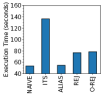
(a) Unbiased.

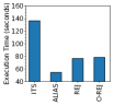
(b) Static.

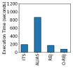
(c) Dynamic.

Figure 1. Effectiveness of sampling methods.

Figure 1 presents the experiment results of the sequential execution with variant sampling methods on different RW types. We have the following findings. First, the NAIVE sampling method performs the best on unbiased RW as it has no initialization phase. Second, among static methods, the ALIAS sampling method outperforms others because its generation phase has lower time complexity. However, ALIAS runs much slower than other methods on dynamic RW since its initialization cost is high in practice. Third, O-REJ performs well on dynamic RW since it does not have the initialization phase. Fourth, we can observe that the cost of evaluating dynamic RW is significantly expensive than that of unbiased and static RW because of the initialization phase (if exists) at each step.

Observation 2. Sampling methods have an important impact on the performance and no sampling method can dominate on all cases. Generally, dynamic RW is expensive than unbiased and static RW.

3.2. System Implications

Based on the profiling results, we can categorize the cost of evaluating RW queries into two classes, that of computing $p(e)$ and that of sampling an edge. As the former is determined by the RW algorithms (i.e., algorithm-specific), our framework targets at accelerating the latter operation. Moreover, we have the following implications for the design and implementation of ThunderRW. First, we need to develop mechanisms to reduce the cache stalls. Our profiling results show that in-memory computation of common RW algorithms suffer severe performance issues due to the irregular memory accesses. None of previous random walk frameworks (Pandey et al., [n.d.]; Wang et al., 2020; Yang et al., 2019) address the problem. On the other hand, there are massive queries in random walk workloads, but the memory bandwidth is under-utilized. Inspired by previous work on accelerating multiple index lookups in database systems with prefetching (Chen et al., 2007; Kocberber et al., 2015), there are opportunities for prefetching and interleaving executions among different queries.

Second, there is a need to support multiple sampling methods. However, existing frameworks support one sampling method only and generally regard all RW as dynamic (e.g., C-SAW), while (1) the sampling method has an important impact on the performance and none of them can dominate on all cases; and (2) the cost of evaluating dynamic RW is generally much more expensive than that of unbiased and static RW.

4. ThunderRW Abstraction

In this section, we present the abstraction of the computation in ThunderRW.

4.1. Step-centric Model

To abstract the computation of RW algorithms, we propose the step-centric model in this paper. We observe that RW algorithms are built upon a number of RW queries rather than a single query. In spite of limited intra-query parallelism, there is abundant inter-query parallelism in RW-algorithms as each RW query can be executed independently. Therefore, our step-centric model abstracts the computation of RW algorithms from the perspective of queries to exploit the inter-query parallelism.

Specifically, we model the computation from the local view of moving one step of a query $Q$. Then, we abstract a step of $Q$ into the Gather-Move-Update (GMU) operations to characterize the common structure of RW algorithms. With the step-centric model, users develop RW algorithms by ”thinking like a walker”. They focus on defining functions setting the transition probability of $e\in E_{v}$ and updating states of $Q$ at each step, while the framework facilitates applying user-defined step-oriented functions to RW queries.

4.2. Step-centric Programming

Input: a graph $G$ and a set $\mathbb{Q}$ of random walk queries;

Output: the walk sequences of each query in $\mathbb{Q}$;

1 foreach $Q\in\mathbb{Q}$ do

2       do

3             $C\leftarrow$ Gather($G$, $Q$, Weight);

4             $e\leftarrow$ Move($G$, $Q$, $C$);

5             $stop\leftarrow$ Update($Q$, $e$);

6            

7      while $stop$ is false;

8return $\mathbb{Q}$;

9

10Function Gather($G,Q$, Weight)

11       $C\leftarrow\{\}$;

12       foreach $e\in E_{Q.cur}$ do

13             Add Weight($Q$, $e$) to $C$;

14      $C\leftarrow$ execute initialization phase of a given sampling method on $C$;

15       return $C$;

16      

17

18Function Move($G,Q,C$)

19       Select an edge $e(Q.cur,v)\in E_{Q.cur}$ based on $C$ and add $v$ to $Q$;

20       return $e(Q.cur,v)$;

21      

Algorithm 2 ThunderRW Framework

Framework. Algorithm 2 gives an overview of ThunderRW. Lines 1-6 execute each query one-by-one. Lines 3-5 factor one step into three functions based on the step-centric model. Gather collects the transition probabilities of edges adjacent to $Q.cur$. It loops over $E_{Q.cur}$, applies Weight, a user-defined function, to each edge $e$ and add the transition probability of $e$ to $C$ (Lines 10-11). Then, Line 12 executes the initialization phase of a given sampling method to update $C$. Move picks an edge based on $C$ and moves $Q$ along the selected edge (Lines 14-16). As random memory accesses in the system space (i.e., the framework excluding user-defined functions) are mainly in Move, we apply step-interleaving techniques to optimize its performance (see Section 5). Finally, Line 5 invokes Update, a user-defined function, to update states of $Q$ based on the movement. The return value of Update decides whether $Q$ should be terminated.

The framework described in Algorithm 2 can support unbiased, static and dynamic RW with different sampling methods. Furthermore, we optimize the execution flow of ThunderRW based on the RW type and the selected sampling method. The transition probability of static RW is fixed during the execution. In that case, ThunderRW omits the Gather operation but introducing a preprocessing step to reduce the runtime cost, which obtains transition probabilities in the system initialization. Algorithm 3 presents the preprocessing for static RW. Given a vertex $v$, Lines 3-4 loop over each edge $e$ in $E_{v}$ and apply the Weight function to $e$ to obtain the transition probability. As the probability does not rely on a query, we set $Q$ as null. After that, Lines 5-6 perform the initialization phase of a given sampling method on $C_{v}$ and store $C_{v}$ for the usage in the query execution. As such, we can load $C_{Q.cur}$ directly without Gather for static RW in Algorithm 2.

Input: a graph $G$;

Output: the transition probabilities $C_{v}$ on $E_{v}$ for each vertex $v$;

1 foreach $v\in V(G)$ do

2       $C_{v}\leftarrow\{\}$;

3       foreach $e\in E_{v}$ do

4             Add Weight($null$, $e$) to $C_{v}$;

5      $C_{v}\leftarrow$ execute initialization phase of a given sampling method on $C_{v}$;

6       Store $C_{v}$ for the usage in query execution.

Algorithm 3 Preprocessing for Static Random Walk

Moreover, the NAIVE and O-REJ sampling methods have no initialization phase as discussed in Section 2.3. Hence, we do not need to collect the transition probability for initialization. As such, ThunderRW skips both the preprocessing step and the Gather operation in the execution if NAIVE or O-REJ is used.

Application Programming Interfaces (APIs). ThunderRW provides two kinds of APIs, which include hyperparameters and user-defined functions. Users develop their RW algorithms in two steps. Firstly, set the RW type and the sampling method via hyperparameters walker_type and sampling_method, respectively. Secondly, define the Weight and Update functions. The Weight function specifies the relative chance of an edge being selected. The Update function modifies states of $Q$ given the selected edge. If its return value is true, then the framework terminates $Q$. Otherwise, $Q$ continues walking on $G$. When using O-REJ, users need to implement the MaxWeight function to set the maximum value of the transition probability. We present an example in the following.

⬇

1WalkerType walker_type = WalkerType::Dynamic;

2SamplingMethod sampling_method = SamplingMethod::O-REJ;

3double Weight(Walker Q, Edge e) {

4 if (Q.length == 0) return max(1.0 / a, 1.0, 1.0 / b);

5 else if (e.dst == Q.prev) return 1.0 / a;

6 else if (IsNeighbor(e.dst, Q.prev)) return 1.0;

7 else return 1.0 / b;

8}

9bool Update(Walker Q, Edge e) {

10 return Q.length == target_length;

11}

12double MaxWeight() {

13 return max(1.0 / a, 1.0, 1.0 / b);

14}

Example 4.1.

List LABEL:list:node2vec shows the sample code of Node2Vec, which is dynamic. As the maximum value can be easily determined by the parameters $a$ and $b$, we use O-REJ to avoid scanning each edge adjacent to $Q.cur$ at each step. Thus, we set sampling_method to O-REJ and implement MaxWeight. The Weight function is configured based on Equation 1. Once the length of $Q$ meets the target length, we terminate it.

ThunderRW applies user-defined functions to RW queries, and evaluates the queries based on RW type and selected sampling method in parallel. Thus, users can easily implement customized RW algorithms with ThunderRW, which significantly reduces the engineering effort. For example, users write only around ten lines of code to implement Node2Vec as shown in Example 4.1.

Parallelization. RW algorithms contain massive random walk queries each of which can be completed independently and rapidly. Therefore, ThunderRW adopts the static scheduling method to keep load balancing among workers. Specifically, we regard each thread as a worker and evenly assign $\mathbb{Q}$ to the workers. A worker independently executes the assigned queries with Algorithm 2. Our experiment results show that the simple scheduling method achieves good performance.

4.3. Analysis

In this subsection, we analyze the space and time cost of Algorithm 2 on different RW types with variant sampling methods. As the cost of Weight and Update is determined by users’ implementation, we assume their cost is a constant value for the ease of analysis.

Table 3. The time complexity of ThunderRW on different random walk types with variant sampling methods

Method	Unbiased	Static	Dynamic
NAIVE	$O(T)$	N/A	N/A
ITS	$O(|E|+T\times\log d_{avg})$	Same as unbiased	$O(T\times(d_{avg}+\log d_{avg}))$
ALIAS	$O(|E|+T)$	Same as unbiased	$O(T\times(d_{avg}+1))$
REJ	$O(|E|+T\times\mathbb{E})$	Same as unbiased	$O(T\times(d_{avg}+\mathbb{E}))$
O-REJ	$O(T\times\mathbb{E})$	Same as unbiased	Same as unbiased

Space. The space for storing the graph is $O(|E|+|V|)$, and that for maintaining the output is $O(\sum_{Q\in\mathbb{Q}}|Q|)$. Gather in Algorithm 2 requires $O(d_{max})$ space to store $C$ where $d_{max}$ is the max degree value of $G$. Suppose that ThunderRW has $n$ threads. Then, the memory cost is $O(n\times d_{max})$. When there is a preprocessing step, the memory cost of ITS and ALIAS is $O(|E|)$, while that of REJ is $O(|V|)$ based on the analysis in Section 2.3.

Time. Given a sampling method, $\alpha$ and $\beta$ denote the cost of its initialization phase and generation phase, respectively. Let $d_{avg}$ represent the average degree of $G$. Thus, the cost of Gather in Algorithm 2 is $d_{avg}+\alpha$, and that of Move is $\beta$. For static RW, the preprocessing cost is $\sum_{v\in V}(d_{v}+\alpha)$, while the cost of processing one step is $\beta$ as it does not conduct Gather during execution. From Section 2.3 we can get the value of $\alpha$ and $\beta$ for the sampling methods. Support that $T=\sum_{Q\in\mathbb{Q}}|Q|$, which is the total number of steps of all queries. Table 3 summarizes the time complexity on different RW types with variant sampling methods.

As shown in the table, NAIVE supports unbiased RW only. For ITS, ALIAS and REJ, the cost on unbiased and static RW consists of the preprocessing cost and the execution cost. Because RW algorithms can have massive RW queries with a long length, the execution cost is generally much more expensive than the preprocessing cost. As O-REJ has no initialization phase, it neither performs the preprocessing for unbiased and static RW nor executes Gather for dynamic RW. Thus, the time complexity is the same for the three RW types.

Recommendation. From the analysis, we have the following guidelines for setting sampling methods for users: (1) NAIVE is the best sampling method for unbiased RW; (2) ALIAS is a good choice for static RW since the execution time is generally longer than the preprocessing time; and (3) if we can set a reasonable max value for the transition probability, then use O-REJ for dynamic RW. Users can easily tell the RW type based on the properties of transition probability. To further ease the programming efforts, we set the default sampling method of unbiased, static and dynamic RW to NAIVE, ALIAS and ITS, respectively. We use ITS instead of ALIAS for dynamic RW because the initialization cost of ALIAS at each step is much more than that of ITS in practice. If users can set a good max value for the transition probability, then they can select O-REJ for dynamic RW.

5. Step-Interleaving

In this section, we present the step interleaving technique, which reduces the pipeline stall caused by random memory accesses.

5.1. General Idea

Based on the step-centric model, ThunderRW processes a step of a query $Q$ with the GMU operations. According to the profiling results in Section 3, there can be two main sources for random memory accesses under the model. First, the Move operation picks an edge randomly and moves $Q$ along the selected edge. Second, the operations in user-defined functions can introduce cache misses, for example, the distance check operation in Node2Vec. As operations in the user space (i.e., user-defined functions) are determined by RW algorithms, and can be very flexible, we target at memory issues incurred by the system (i.e., the Move operation). Motivated by the profiling result, we propose to use the software prefectching technique (Lee et al., 2012) to accelerate in-memory computation of ThunderRW. However, a step of a query $Q$ does not have enough computation workload to hide memory access latency because steps of $Q$ have dependency relationship. Therefore, we propose to hide memory access latency via executing steps of different queries alternately.

Specifically, given a sequence of operations in Move, we decompose them into multiple stages such that the computation of a stage consumes the data generated by previous stages and it retrieves the data for the subsequent stages if necessary. We execute a group of queries simultaneously. Once a stage of a query $Q$ completes, we switch to stages of other queries in the group. We resume the execution of $Q$ when stages of other queries complete. In such a way we hide the memory access latency in a single query and keep CPUs busy. We call this approach step interleaving.

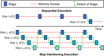
Figure 2. Sequential versus step interleaving.

Example 5.1.

Figure 2 presents an example where a step is divided into four stages. If executing a query step-by-step sequentially, then CPUs are frequently stalled due to memory access. Even with prefetching, the computation of a stage cannot hide the memory access latency. In contrast, the step interleaving hides the memory access latency by executing steps of different queries alternately.

Let’s perform a simple back-of-envelop calculation on the performance gain of interleaving execution. Given a group containing $k$ queries, we assume that Move of each query executes the same number of stages and the cost $W_{C}$ of each stage is the same for the ease of analysis. Suppose that there are $m$ stages with memory access and $\overline{m}$ without. $W_{L}$ denotes the latency of memory access. Then, the cost of moving a step for the queries in sequential is equal to $W_{0}=k((m+\overline{m})W_{C}+mW_{L}$). Let $W_{S}$ denote the cost of switching. The cost of Move with step interleaving is $W_{1}=k((m+\overline{m})(W_{C}+W_{S})+m(\max(W_{L}-kW_{S}-(k-1)W_{C},0))$ where the last term calculates whether step interleaving hides memory access latency. Therefore, the gain of step interleaving for a step of $k$ queries can be estimated by Equation 2 where $W_{hide}=\max(W_{L}-kW_{S}-(k-1)W_{C},0)$.

(2) $$W_{gain} =(W_{0}-W_{1})/k$$

$$=mW_{L}-(m+\overline{m})W_{S}-mW_{hide}.$$

From Equation 2, we can see that step interleaving requires an efficient switch mechanism to reduce the overhead $W_{S}$ of performing switching, and enough workload to overlap the memory access latency $W_{hide}$.

5.2. Stage Dependency Graph

We design the stage dependency graph (SDG) to model stages of a sequence of operations in a step. Each node in SDG is a stage containing a set of operations and edges represent the dependency relationship among them. Given the sequence of operations, we build SDG in two steps, abstracting stages (nodes) and extracting dependency relationships (edges).

Defining stages: As we hide memory access latency by switching the execution of queries, the constraint on stages is that each stage contains at most one memory access operation and the operations consuming the data are in subsequent stages. Note that we view the operation containing jump operation as a single stage for the ease of the implementation of switching. We present an example in the following.

Table 4. Stages of Move with ALIAS and REJ ($v=Q.cur$).

Stage	ALIAS
$S_{0}$	$O_{0}$: Load $d_{v}$.
$S_{1}$	$O_{1}$: Generate an int random num $x$ in $[0,d_{v})$.
	$O_{2}$: Generate a real random num $y$ in $[0,1)$.
	$O_{3}$: Load $C[x]=(H[x],A[x])$.
$S_{2}$	$O_{4}$: If $y<H[x]$, $v^{\prime}=A[x].first$; Else $v^{\prime}=A[x].second$.
	$O_{5}$: Add $v^{\prime}$ to $Q$ and return $e(v,v^{\prime})$.
Stage	REJ
$S_{0}$	$O_{0}$: Load $d_{v}$.
$S_{1}$	$O_{1}$: Load the maximum value $p_{v}^{*}$.
$S_{2}$	$O_{2}$: Generate an int random num $x$ in $[0,d_{v})$.
	$O_{3}$: Generate a real random num $y$ in $[0,p_{v}^{*})$.
	$O_{4}$: Load $C[x]=p$.
$S_{3}$	$O_{5}$: If $y>C[x]$, jump to $O_{2}$; Else jump to $O_{6}$.
$S_{4}$	$O_{6}$: Load $e(v,v^{\prime})=E_{v}[x]$.
$S_{5}$	$O_{7}$: Add $v^{\prime}$ to $Q$ and return $e(v,v^{\prime})$.

Example 5.2.

The right column of Table 4 illustrates the sequence of operations in the Move function with the ALIAS and REJ sampling methods, respectively, to perform the neighbor selection. The left column lists stages. For example, $S_{0}$ of ALIAS loads $d_{v}$ consumed in $O_{1}$ of $S_{1}$. $O_{5}$ in REJ has the jump operation. Therefore, we regard it as a separate stage.

Defining edges: Next, we add edges among nodes in SDG based on their dependency relationships. Given stages $S$ and $S^{\prime}$, if there is a dependency relationship between $S$ and $S^{\prime}$, we add an edge from $S$ to $S^{\prime}$. The edges are categorized into three types, memory dependency, computation dependency and control dependency. We call the first two relationship as data dependency. More specifically, if $S^{\prime}$ consumes the data loaded from memory by $S$, then the edge type is memory dependency. Otherwise, $S^{\prime}$ depends on the data computed by $S$ and the edge type is computation dependency. The data leading to the dependency is attached to each edge as properties. Furthermore, if $S$ contains the operation jumping to $S^{\prime}$, we add the control dependency from $S$ to $S^{\prime}$. SDG allows that there are multiple edges (i.e., dependency relationships) between nodes. If we only consider data dependency, SDG is a directed acyclic graph (DAG), while the control dependency can generate cycles in SDG.

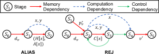
Figure 3. Stage dependency graph.

Example 5.3.

Continuing with Example 5.2, Figure 3 shows SDGs. In SDG of ALIAS, $S_{2}$ relies on $x,y$, which are random numbers generated by $S_{1}$, while $(H[x],A[x])$ is the data retrieved from memory. As such, $S_{1}$ and $S_{2}$ have both memory and computation dependency relationships. SDG of ALIAS is a DAG because there is no control dependency. In contrast, there is a cycle containing $S_{2}$ and $S_{3}$ in SDG of REJ because of the control dependency.

In summary, SDG is a methodology to abstract stages from a sequence of operations in Move and model the dependency relationship among them. Note that the stage design of MOVE does not require user input but it is implemented in the system space.

5.3. State Switch Mechanism

In this subsection, we introduce the implementation of step interleaving under SDG. Based on Equation 2, we need an efficient switch mechanism. For example, using multi-threading is forbidden because the overhead of context switch among threads is in microseconds, whereas the main memory latency is in nanoseconds. As each thread tends to take many RW queries, we switch the execution among stages in a single thread.

We categorize stages of a SDG into two classes based on whether they belong to cycles in SDG, and efficiently handle them in different manners. For stages not in cycles (called non-cycle stages), a query visits them exactly once to complete Move. Given a group of queries $\mathbb{Q}^{\prime}$, we execute them in a coupled manner. Particularly, once a query $Q_{i}\in\mathbb{Q}^{\prime}$ completes a stage $S$, we switch to the next query $Q_{i+1}\in\mathbb{Q}^{\prime}$ to process $S$. After all queries complete $S$, we move to the next stage. In contrast, stages in cycles (called cycle stages) can be visited variant times for different queries. To deal with the irregularity, we process them in a decoupled manner. Specifically, each query $Q$ records the stage $S$ to be executed. When switching to $Q$, we execute $S$, set the next stage of $Q$ based on SDG, and switch to the next query after completing $S$. As a result, each query executes asynchronous.

For data communication between different stages in a query, we create two kinds of ring buffers based on SDG, in which the computation dependency edge indicates the information requiring to be stored. In particular, the task ring is used for data communication across all stages of a query, while the search ring serves to process cycle stages. As we need to explicitly record states of cycle stages and control the switch of them, processing cycle stages not only causes implementation complexities, but also incurs more overhead. Note that the SDGs of NAIVE and ALIAS have no cycle stages because there are no for loops in their generation phases, whereas that of ITS, REJ and O-REJ have. The implementation details are introduced in the appendix.

5.4. Ring Size Tuning

The task ring size $k$ and the search ring size $k^{\prime}$ determine the group size of queries executed simultaneously in a thread, and therefore control memory level parallelism of executing non-cycle stages and cycle stages, respectively. According to Equation 2, we can improve the performance by increasing $k$ to reduce $W_{hide}$. However, $k$ is limited by hardware. Particularly, modern CPUs can issue a limited number of outstanding memory requests, and the L1 data cache size is only tens of kilobytes. Setting $k$ to a large value can evict data before the usage. In ThunderRW, we tune ring sizes by pre-executing a number of queries. We start a RW query from each vertex with the target length as 10 and set the RW type as static. We first select the NAIVE and ALIAS sampling methods, respectively and vary $k$ from $1,2,...,512,1024$ to pick an optimal value $k^{*}$. Next we fix $k$ to $k^{*}$ and vary $k^{\prime}$ from $1,2,...,k^{*}$ to select optimal values for ITS, REJ and O-REJ, respectively.

Input: a graph $G$ and a set $\mathbb{Q}$ of random walk queries;

Output: the walk sequences of each query in $\mathbb{Q}$;

1 Add the first $k$ queries in $\mathbb{Q}$ to $\mathbb{Q}^{\prime}$;

2 $completed\leftarrow 0$, $submitted\leftarrow k$;

3 while $completed<|\mathbb{Q}|$ do

4       $\mathbb{C}\leftarrow\{\}$;

5       for $Q\in\mathbb{Q}^{\prime}$ do

6             $C\leftarrow$Gather($G,Q,\textbf{Weight}$);

7             Add $\mathbb{C}[Q]$ to $C$;

8            

9      

10      $\mathbb{U}\leftarrow$ Move($G,\mathbb{Q}^{\prime},\mathbb{C}$);

11      

12      for $Q\in\mathbb{Q}^{\prime}$ do

13             if Update($Q,\mathbb{U}[Q]$) is true then

14                   Remove $Q$ from $\mathbb{Q}^{\prime}$;

15                   $completed\leftarrow completed+1$;

16                   if $submitted<|\mathbb{Q}|$ then

17                         Get next query $Q^{\prime}$ from $\mathbb{Q}$ and add it to $\mathbb{Q}^{\prime}$;

18                         $submitted\leftarrow submitted+1$;

19                        

20                  

21            

22      

Algorithm 4 ThunderRW using Step Interleaving

5.5. Integration with ThunderRW

Algorithm 4 illustrates our ThunderRW framework using step interleaving. Line 1 adds the first $k$ queries in $\mathbb{Q}$ to $\mathbb{Q}^{\prime}$ where $k$ is the parameter setting the group size. Lines 3-15 repeatedly execute GMU operations on queries in $\mathbb{Q}^{\prime}$ until all queries in $\mathbb{Q}$ complete. Specifically, Lines 5-7 first execute the Gather operation on each query in $\mathbb{Q}^{\prime}$. Next, Line 8 invokes the Move operation using step interleaving to process queries in $\mathbb{Q}^{\prime}$. After that, Lines 9-15 apply the Update operation to all queries in the group. If a query completes, then Lines 11-15 remove it and submit the next query in $\mathbb{Q}$ to $\mathbb{Q}^{\prime}$. Thus, the step interleaving technique can be seamlessly integrated with ThunderRW without changing APIs.

Time and space. The time complexity of Algorithm 4 is the same with the analysis in Section 4.3 because the step interleaving does not change the number of steps moved. Suppose that there are $n$ threads. Then, the memory cost is $O(n\times k\times d_{max})$ in addition to the space storing the graph and the output because each thread has at most $k$ queries in flight.

6. Experiments

We conduct experiments to evaluate the performance of ThunderRW in this section.

6.1. Experimental Setup

We conduct experiments on a Linux server equipped with an Intel Xeon W-2155 CPU and 220GB RAM. The CPU has ten physical cores with hyper-threading disabled for consistent measurement. The sizes of L1, L2 and L3 (last level cache, LLC) caches are 32KB, 1MB and 13.75MB, respectively.

Table 5. Properties of real-world datasets.

Dataset	Name	$|V|$	$|E|$	$d_{avg}$	$d_{max}$	Memory
amazon	am	0.55M	1.85M	3.38	549	0.01GB
youtube	yt	1.14M	2.99M	5.24	28754	0.03GB
us patents	up	3.78M	16.52M	8.74	793	0.17GB
eu-2005	eu	0.86M	19.24M	44.74	68963	0.15GB
amazon-clothing	ac	15.16M	63.33M	4.18	12845	0.35GB
amazon-book	ab	18.29M	102.12M	5.58	58147	0.52GB
livejournal	lj	4.85M	68.99M	28.45	20333	0.54GB
com-orkut	ot	3.07M	117.19M	76.34	33313	0.89GB
wikidata	wk	40.96M	265.20M	6.47	8085513	1.29GB
uk-2002	uk	18.52M	298.11M	32.19	194955	2.30GB
twitter	tw	41.66M	1.21B	58.08	2997487	9.27GB
friendster	fs	65.61M	1.81B	55.17	5214	13.71GB

Datasets. Table 5 lists the statistics of the twelve real-world graphs in our experiments. ab and ac are downloaded from (n.d., 2018), wk is obtained from (n.d., [n.d.]), eu, uk and tw are obtained from (Rossi and Ahmed, 2015), and the other graphs are downloaded from (Leskovec and Krevl, 2014). The datasets are from different categories such as web, social and citation, and have different densities. The number of vertices is ranged from hundreds of thousands to tens of millions, and the number of edges scales from millions to billions. Except am, all the graphs outsize LLC.

Workloads. We study PPR, DeepWalk, Node2Vec and MetaPath to evaluate the performance and generality of competing methods. The settings of the four algorithms are the same as that in Section 3. ab and ac are weighted graphs where weights denote review ratings for products. wk has 1327 distinct labels, which represents the relationship between entities in a knowledge base. The other graphs are unweighted and unlabeled. Given a graph having no labels or weights, we set the weight and label of edges with the same setting as previous work (Yang et al., 2019): (1) We choose a real number from [1, 5) uniformly at random, and assign it to an edge as its weight; and (2) We set the edge label by randomly choosing a label from a set containing five distinct labels.

Comparison. We compare the performance of ThunderRW (called TRW for short) with the following methods.

• BL: Baseline approaches that first load a graph entirely into memory and then execute random walks, the detail of which is presented in Section 3.

• HG: Our homegrown implementation optimizing BL from two aspects: (1) select a suitable sampling method for each algorithm according to the recommendation in Section 4.3; and (2) regard each query as a parallel task with OpenMP.

• GW: GraphWalker (Wang et al., 2020), the state-of-the-art RW framework in a single machine. For the fair of comparison, we configure GraphWalker to execute in-memory, without any disk I/O.

• KK: KnightKing (Yang et al., 2019), the state-of-the-art distributed RW framework. It supports to execute in a single machine.

Table 6. Overall performance comparison (seconds).

	PPR					DeepWalk				Node2vec				MetaPath
Dataset	BL	HG	GW	KK	TRW	BL	HG	KK	TRW	BL	HG	KK	TRW	BL	HG	TRW
am	0.06	0.008	0.42	0.012	0.007	2.16	0.21	0.44	0.07	9.97	0.26	2.08	0.14	0.22	0.018	0.012
yt	0.33	0.04	1.68	0.05	0.015	9.78	0.98	1.93	0.26	853.13	1.30	5.94	1.03	6.18	0.23	0.24
up	1.24	0.13	7.19	0.19	0.07	45.44	4.33	8.41	0.95	369.00	6.20	16.92	4.01	4.88	0.40	0.24
eu	0.16	0.02	0.99	0.03	0.011	8.16	0.82	1.56	0.20	2731.07	1.47	4.43	1.14	90.55	3.18	3.55
ac	4.84	0.51	19.31	0.65	0.19	173.66	17.86	31.88	3.31	6951.12	24.54	87.86	6.26	45.01	2.01	1.69
ab	8.86	0.94	26.74	1.09	0.26	212.80	22.24	40.07	4.01	26231.45	32.04	100.78	7.87	128.35	5.06	4.47
lj	1.69	0.19	7.90	0.23	0.06	55.63	5.44	10.67	1.19	2951.33	9.09	24.95	6.20	18.08	0.94	0.75
ot	1.49	0.16	5.25	0.19	0.04	38.54	3.70	7.97	0.80	5891.28	7.28	15.16	4.82	40.77	1.72	1.57
wk	21.86	2.21	47.05	3.07	0.59	502.27	49.67	95.17	9.26	OOT	68.43	216.24	27.68	5.98	0.54	0.55
uk	6.47	0.69	27.72	0.90	0.24	203.86	20.42	21.40	4.56	12630.01	34.36	94.69	28.68	322.66	12.84	12.56
tw	26.42	2.73	77.12	3.61	1.16	575.43	61.18	115.92	11.13	OOT	130.72	232.41	91.00	OOT	12300.32	9780.20
fs	79.14	8.20	223.81	10.72	4.10	1043.93	108.23	208.45	17.67	OOT	178.15	364.51	120.16	683.05	28.69	25.01

We implement all our methods including BL, HG and TRW in C++. GW and KK are programmed in C++ as well. All the source code is compiled by g++ 8.3.2 with -O3 enabled. BL executes in serial, while the other methods are running on all the cores of the single socket, with one thread per core.

We consider C-SAW (Pandey et al., [n.d.]), the state-of-the-art RW framework on GPUs, as well. However, its open source package supports 4000 queries at most, which cannot handle the workload containing massive queries in the experiment. Previous experiment results (Yang et al., 2019; Wang et al., 2020) show that KK and GW significantly outperform generic graph computing frameworks such as Gemini (Zhu et al., 2016) on RW algorithms. Therefore, our experiment does not involve C-SAW as well as any generic graph computing frameworks.

As for RW algorithms, GW only supports unbiased RW. Thus, we execute PPR without considering edge weights, and evaluate GW on PPR only. Despite that KK studies MetaPath in the original paper (Yang et al., 2019), its open source package cannot handle labeled graphs. As such, it cannot execute MetaPath. In contrast, TRW supports all the four algorithms, which demonstrates its flexibility.

As for sampling methods, BL uses NAIVE for PPR, while adopts ALIAS for the other three algorithms. As discussed in Section 3, building alias tables for dynamic RW in an indexing phase can consume a huge amount of memory. Therefore, in the experiments, BL dynamically computes the alias table (i.e., perform the initialization of ALIAS) at each step of a query, which is the same as the computation flow of TRW for dynamic RW. Different from BL, HG adopts O-REJ for Node2Vec, and ITS for MetaPath. This is because (1) the max value of transition probability of Node2Vec can be easily set as $\max(1,1/a,1/b)$, and O-REJ can avoid scanning the neighbors of $Q.cur$ at each step; and (2) the probability distribution of MetaPath is skewed due to filtering based on labels, which increases the generation cost of rejection sampling, and the initialization phase of ITS is much faster than that of ALIAS in practice. TRW adopts the same sampling method as HG for each algorithm.

Ring Size Setting. We tune the ring size with the method in Section 5.4. Despite that the graphs have variant structures, the optimal setting for them is close. First, the optimal value for the graphs except am is $k=64$ and $k^{\prime}=32$ because the optimal ring size is closely related to the instructions available for computation, the switch overhead, the memory access latency, and the maximum number of outstanding memory requests, which are determined by the program and hardwares. Second, the optimal value for am is $k=32$ and $k^{\prime}=32$ as am fits in LLC and the memory access latency is smaller than that of the other graphs. Additionally, the tuning process is very efficient, which takes less than one minute for most of the graphs. Even for fs with more than 1.8 billion edges, the tuning is completed with around four minutes.

Metrics. The total time is the elapsed time on evaluating RW algorithms without counting the time on loading data from the disk. For static random walk, the total time consists of the preprocessing time, which is the time spent on the preprocessing, and the execution time, which is the time spent on executing queries. To complete experiments in a reasonable time, we set the time limit for each algorithm as eight hours. If an algorithm cannot be completed within the limit, we terminate it and record the execution time as OOT (i.e., out-of-time). We measure the throughput (steps per second) by dividing the number of steps of all queries by the execution time. To provide more insights, we adopt Intel Vtune Profiler to examine the pipeline slot utilization and use Linux Perf to examine the instructions per step and cycles per step, which are the number of instructions and the number of cycles on one step, respectively.

Supplement experiments. More experiment results including the impact of ring sizes, memory bandwidth utilization, the effectiveness of prefetching data to different cache levels, the impact of the step interleaving on existing systems and the comparison with AMAC (Kocberber et al., 2015) are presented in the appendix.

6.2. Overall Comparison

Table 6 gives an overall comparison of competing methods on the four RW algorithms. Although GW is parallel, it runs slower than BL, the sequential baseline algorithm. KK runs faster than GW and BL, but slower than HG because (1) the framework incurs extra overhead compared with HG; and (2) HG adopts an appropriate sampling method for each algorithm. TRW runs 54.6-131.7X and 1.7-14.6X faster than GW and KK, respectively.

Benefiting from parallelization, HG achieves 7.5-10.5X speedup over BL on PPR and DeepWalk. Moreover, HG runs 38.3-1857.9X and 11.1-28.5X faster than BL on Node2Vec and MetaPath, respectively, because HG adopts O-REJ sampling for Node2Vec, which avoids scanning the neighbors of $Q.cur$ at each step, and uses ITS sampling for MetaPath, the initialization phase of which is more efficient than that of ALIAS in practice. TRW runs 8.6-3333.1X faster than BL. Even compared with HG, TRW achives up to 6.1X speedup benefiting from our step-centric model and step interleaving technique. As MetaPath is dynamic and both TRW and HG use ITS sampling, the gather operation at each step dominates the cost. Still, MetaPath on ThunderRW outperforms that on HG for nine out of twelve graphs, and is slightly slower on the other three graphs. tw is dense but highly skewed (as shown in Table 5) and the vertices with high degrees are frequently visited. Consequently, the execution time on MetaPath against tw is much longer than that on other graphs.

In summary, ThunderRW significantly outperforms state-of-the-art frameworks and homegrown solutions (e.g., BL takes more than eight hours for Node2Vec on tw, while TRW completes the algorithm in two minutes). Furthermore, ThunderRW saves a lot of engineering effort on the implementation and parallelization of RW algorithms compared with BL and HG.

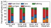
(a) Pipeline slot breakdown.

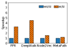
(b) Speedup.

Figure 4. Vary RW-algorithms on lj.

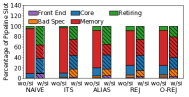
(a) Pipeline slot breakdown.

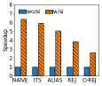
(b) Speedup.

Figure 5. Vary sampling methods on lj.

6.3. Evaluation of Step Interleaving

We evaluate the effectiveness of step interleaving in this subsection. For brevity, we use lj as the representative graph by default.

Varying RW algorithms. We first evaluate the effectiveness of step interleaving on different RW algorithms. Figure 4 presents the pipeline slot breakdown and speedup among the RW algorithms. wo/si and w/si denote ThunderRW without and with the step interleaving technique, respectively. Enabling step interleaving drastically reduces memory bound on PPR and DeepWalk, and improves the instruction retirement. Correspondingly, w/si achieves significant speedup over wo/si in Figure 4(b). The speedup on PPR is lower than that on DeepWalk because PPR issues all queries from a given vertex and the expected length of a query is 5, which by default exhibits better memory locality than DeepWalk. The memory bound on Node2Vec is reduced from around 60% to 40% because the Weight function checks whether two vertices are neighbors with a binary search, which causes a number of random memory access. The speedup on MetaPath is small because MetaPath is dynamic and the gather operation dominates the cost at each step.

Varying sampling methods. We next examine the performance of step interleaving on variant sampling methods. As the gather operation dominates the cost on dynamic random walk, we focus on unbiased and static random walk. Particularly, we use DeepWalk as the representative RW algorithm and evaluate it with the five sampling methods in Section 2.3, respectively. When adopting NAIVE, we regard DeepWalk as unbiased random walk (i.e., without considering edge weight). Figure 5 presents the pipeline slot breakdown and speedup on lj with variant sampling methods. We can see that the step interleaving technique significantly reduces memory bound on all the five sampling methods and achieves remarkable speedup. The results demonstrate both the generality and effectiveness of the step interleaving technique.

Varying datasets. To explore the impact of graph structures on the performance, we evaluate the speedup of enabling step interleaving for DeepWalk on different datasets. Figure 6 presents the experiment results. The speedup on am and yt is smaller than that on other graphs because am can fit in LLC, and yt is only two times larger than LLC. The speedup on eu and uk is lower than the other graphs that are much larger than LLC since eu and uk have dense communities (e.g., uk has a clique containing around 1000 vertices (Chang, 2019)), and RW queries exhibit good memory locality. In contrast, the speedup on ac and ab is generally higher than the other graphs because they are bipartite graphs and very sparse, and RW queries have poor memory locality. In summary, the optimization tends to achieve higher speedup on large and sparse graphs than small graphs and graphs with dense community structures because RW queries have poorer memory locality on the former one. Nevertheless, the optimization brings up to 3X speedup even on graphs entirely fitting in LLC (i.e., am) since L1 cache is only tens of kilobytes, but around ten times faster than LLC, and the step interleaving directly fetches the data to L1 cache.

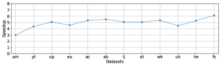
Figure 6. Vary datasets for DeepWalk.

6.4. Scalability Evaluation

In this section, we evaluate the scalability of ThunderRW. By default, we execute $10^{7}$ RW queries on lj with the target length as 80. Each query starts from a vertex selected from the graph randomly. We first evaluate the throughput in terms of steps per second with the number of queries and the length of queries varying, respectively. In that case, we set the RW as static and use the ALIAS sampling method as the representative. Next, we evaluate the speedup with the number of threads varying. When setting the RW as unbiased, we use the NAIVE sampling method, while we examine the speedup on ITS, ALIAS, REJ and O-REJ, respectively, when setting the RW as static and dynamic.

Varying number and length of queries. Figure 7(a) presents the throughput with the number of queries varying from $10^{2}$ to $10^{7}$. For $10^{2}-10^{4}$ queries, the execution time is very short and the start up and shut down time can dominate it. For example, for $10^{2}$ queries, each thread spends less than 0.1 ms on performing random walks, while the execution time is around 2 ms because of the cost on resource (e.g., memory and threads) initialization and release. As a result, the benefit of the optimization is limited, and the throughput is lower than that with a large number of queries. The throughput is more than $3\times 10^{8}$ and keeps stable with the number of queries varying from $10^{6}$ to $10^{7}$. Figure 7(b) presents the throughput with the length of queries varying from 5 to 160. The throughput is steady. In summary, ThunderRW has good scalability in terms of the number and length of queries.

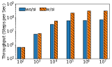
(a) Varying number of queries.

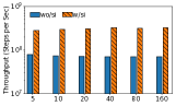
(b) Varying length of queries.

Figure 7. Throughput on lj with number and length of queries varying.

Varying number of threads. Figure 8 shows the speedup with the number of threads varying from 1 to 10 (i.e., the number of cores in the machine). For all the five sampling methods on unbiased/static RW, ThunderRW achieves nearly linear speedup with the number of threads as shown in Figure 8(a). Particularly, when the number of threads is 10, the speedup is from 8.8X to 9.6X. Figure 8(b) presents the speedup on dynamic RW. The speedup is from 7.8X to 9.0X. Overall, ThunderRW achieves good scalability in terms of the number of threads.

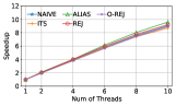
(a) Unbiased/static RW.

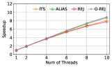
(b) Dynamic RW.

Figure 8. Speedup on lj with number of threads varying.

6.5. Generality Evaluation

To evaluate the generality of ThunderRW, we repeat the first experiment in Section 6.4 on a machine equipped with an Intel Xeon Gold 6246R CPU, which has 16 physical cores. The sizes of L1, L2 and LLC caches are 32KB, 1MB and 35.75MB, respectively. Additionally, the CPU is based on the Cascade Lake microarchitecture, while that used in other experiments is based on Skylake. As the CPU has 16 physical cores, we set the number of workers as 16. As shown in Figure 9, enabling the optimization significantly improves the throughput. Moreover, using the new CPU increases the throughput, for example, when the length of queries is 160, the throughput grows from $3\times 10^{8}$ to $4.1\times 10^{8}$. The experiment results show that the techniques proposed in this paper are generic to different architectures.

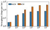
(a) Varying number of queries.

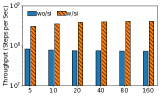
(b) Varying length of queries.

Figure 9. Throughput on lj with number and length of queries varying on processors with different architectures.

6.6. Discussions

ThunderRW regards a step of a query as a parallel task unit, which parallelizes the computation from the perspective of queries instead of the graph data. As RW algorithms consist of massive queries and the cost of moving a step is extremely small (e.g., around 34 ns for DeepWalk on lj), there are a large number of small parallel tasks, which can be easily parallelized. As such, the parallelization of ThunderRW can achieve significant speedup over the sequential despite that graph structures are complex and flexible. Moreover, the sampling method has an important impact on the performance, and therefore providing variant sampling methods is essential.

The step interleaving technique executes different queries alternately to reduce memory bound incurred by random memory accesses. Its effectiveness is closely related to the memory locality of workloads, which is determined by RW algorithms and graph structures. In general, the optimization tends to achieve higher speedup on large and sparse graphs than small graphs and graphs with dense community structures because RW queries have poorer memory locality on the former graphs. Nevertheless, the random memory access is a common issue for RW algorithms since (1) graphs are much larger than cache sizes; and (2) RW queries wander randomly in the graph. Thus, the step interleaving can achieve significant speedup even on graphs entirely fitting LLC.

However, the speedup achieved by the step interleaving on high order RW algorithms can be lower than that on first order algorithms. First, the operations in user-defined functions can introduce random memory accesses. Despite that, the optimization still brings 1.2-4.3X speedup on Node2Vec. Second, the Gather operation dominates the cost at each step when performing it in run time.

7. Conclusion

In this paper, we propose ThunderRW, an efficient in-memory RW engine on which users can easily implement customized RW algorithms. We design a step-centric model to abstract the computation from the local view of moving one step of a query. Based on the model, we propose the step interleaving technique to hide memory access latency by executing multiple queries alternately. We implement four representative RW algorithms including PPR, DeepWalk, Node2Vec and MetaPath with our framework. Experimental results show that ThunderRW outperforms state-of-the-art RW frameworks by up to one order of magnitude and the step interleaving reduces the memory bound from 73.1% to 15.0%. Currently, we implement the step interleaving technique in ThunderRW by explicitly and manually storing and restoring states of each query. An interesting future work is to implement the method with coroutines, which is an efficient technique supporting interleaved execution (Jonathan et al., 2018; Psaropoulos et al., 2017; He et al., 2020).

Appendix A Other Profiling Results

In this section, we evaluate the impact of varying the length and the number of queries, respectively. We use a micro benchmark that assembles the access pattern of RWs and also we can control the parameters easily. Particularly, we set the number of queries as $10^{7}$ and configure the target length as 80 by default. Each query starts from a vertex randomly selected from the graph. We use the ALIAS sampling method to perform the queries. We first evaluate the impact of varying the length from 5 to 160, and then examine the performance of varying the number of queries from $10^{2}$ to $10^{8}$.

Tables 7 and 8 present the results with the length of queries varying from 5 to 160 and the number of queries varying from $10^{2}$ to $10^{8}$ on the livejournal graph, respectively. We can see that the memory bound is consistently above 60% despite the variance in the length and number of queries. With the length (or the number of queries) increasing, the memory bound grows slightly. The memory bandwidth utilization is also far from the maximum bandwidth in all test cases. In summary the in-memory computation of RW algorithms suffers severe performance issues due to memory stalls caused by cache misses and under-utilizes the memory bandwidth regardless of the length and number of queries.

Table 7. Pipeline slot breakdown and memory bandwidth with the length of queries varying.

Length of Queries	Front End	Bad Spec	Core	Memory	Retiring	Memory Bandwidth
5	3.6%	5.5%	16.6%	61.3%	13.0%	7.7GB/s
10	2.7%	4.0%	18.5%	63.4%	11.2%	6.6GB/s
20	2.7%	4.1%	18.1%	64.0%	11.1%	6.0GB/s
40	2.5%	4.0%	18.1%	64.5%	10.9%	5.8GB/s
80	2.3%	3.7%	18.6%	64.8%	10.6%	5.6GB/s
160	2.3%	3.6%	18.5%	65%	10.5%	5.6GB/s

Table 8. Pipeline slot breakdown and memory bandwidth with the number of queries varying.

Num of Queries	Front End	Bad Spec	Core	Memory	Retiring	Memory Bandwidth
$10^{2}$	4.1%	2.6%	16.5%	66.4%	10.4%	5.9GB/s
$10^{3}$	4.5%	7.4%	12.1%	63.8%	12.2%	8.0GB/s
$10^{4}$	4.4%	6.9%	12.7%	64.3%	11.8%	6.6GB/s
$10^{5}$	4.0%	6.2%	16.5%	60.9%	12.4%	6.0GB/s
$10^{6}$	2.7%	4.1%	19.0%	63.2%	11.0%	5.8GB/s
$10^{7}$	2.3%	3.7%	18.6%	64.8%	10.6%	5.6GB/s
$10^{8}$	2.3%	3.6%	18.5%	65.1%	10.5%	5.6GB/s

Appendix B Other Implementation Details

In this section, we present the implementation details of the stage switch mechanism, the graph storage, the walker management and the input/output of the framework.

Stage switch. Continuing with Example 5.3, we use Move with the REJ sampling method to demonstrate the implementation of stage switch. Algorithm 5 presents the details where $\mathbb{Q}^{\prime}$ is a group of queries and $\mathbb{C}$ maintains the transition probability $C$ for each $Q\in\mathbb{Q}^{\prime}$. Line 2 creates a task ring $TR$ with $|\mathbb{Q}^{\prime}|$ slots. Each slot records states of a query $Q\in\mathbb{Q}^{\prime}$. The load operations are replaced with the PREFETCH operations. We process a non-cycle stage $S$ in SDG with a for loop where all queries evaluate $S$ one by one. For example, Lines 4-5 deal with $S_{0}$ in which we fetch the degree of $Q.cur$ for each $Q\in\mathbb{Q}^{\prime}$. The Search function handles cycle stages. Line 16 first creates a search ring $SR$ with $k^{\prime}$ slots to process cycle stages. If a slot $R\in SR$ is empty and there are queries in $TR$ not submitted to $SR$ (Line 20), Lines 21-23 submit a query $Q$ to $SR$ and initialize the slot $R$. If the stage is $S_{2}$, Lines 25-27 perform the operations in $S_{2}$. Moreover, Line 28 sets $R.S$ to $S_{3}$ and stores $x,y$ because the next stage is $S_{3}$ and $S_{3}$ depends on the value of $x,y$ according to SDG. When $S_{3}$ is completed, we write $x$ to $TR$ because $S_{4}$ consumes it as shown in SDG. Lines 18-34 repeat the process until all queries jump out the cycle. Lines 9-13 continue the computation with values generated by Search. Line 14 returns $\mathbb{U}$ that maintains the selected edge for each query.

1 Function Move($G,\mathbb{Q}^{\prime},\mathbb{C}$)

2       Initialize a task ring $TR$ each slot of which corresponds to $Q\in\mathbb{Q}^{\prime}$;

3       Initialize $\mathbb{U}$ as $\{\}$ to store the selected edge for $Q\in\mathbb{Q}^{\prime}$;

       /* Stage $S_{0}$. */

4       foreach $Q\in\mathbb{Q}^{\prime}$ do

5             PREFETCH $d_{v}$ where $v=Q.cur$;

6            

      /* Stage $S_{1}$. */

7       foreach $Q\in\mathbb{Q}^{\prime}$ do

8             PREFETCH $p_{v}^{*}$ where $v=Q.cur$;

9            

10      Search($\mathbb{C},TR$);

       /* Stage $S_{4}$. */

11       foreach $Q\in\mathbb{Q}^{\prime}$ do

12             PREFETCH $E_{v}[TR[Q].x]$ where $v=Q.cur$;

13            

      /* Stage $S_{5}$. */

14       foreach $Q\in\mathbb{Q}^{\prime}$ do

15             Add $v^{\prime}$ to $Q$ where $v=Q.cur$ and $e(v,v^{\prime})=E_{v}[TR[Q].x]$;

16             Set $\mathbb{U}[Q]$ to $e(v,v^{\prime})$;

17            

18      

19      return $\mathbb{U}$;

20      

21

22Function Search($\mathbb{C},TR$)

23       Initialize a search ring $SR$ with $k^{\prime}$ slots where $k^{\prime}\leqslant|TR|$;

24       $submitted,completed,index\leftarrow 0$;

25       while $completed<|TR|$ do

26             $R\leftarrow SR[index]$;

27             if $R.S=null$ and $submitted<|TR|$ then

28                   Get next slot $R^{\prime}\in TR$ and set $v$ to $R^{\prime}.Q.cur$;

29                   Set $R.Q$, $R.S$, $R.d$ and $R.p^{*}$ to $R^{\prime}.Q$, $S_{2}$, $d_{v}$ and $p_{v}^{*}$, respectively;

30                   $submitted\leftarrow submitted+1$;

31                  

            /* Stage $S_{2}$. */

32             else if $R.S=S_{2}$ then

33                   Generate an int random number $x$ in $[0,R.d)$;

34                   Generate a real random number $y$ in $[0,R.p^{*})$;

35                   PREFETCH $C[x]$ where $C=\mathbb{C}[R.Q]$;

36                   Set $R.S$, $R.x$ and $R.y$ to $S_{3}$, $x$ and $y$, respectively;

37                  

            /* Stage $S_{3}$. */

38             else if $R.S=S_{3}$ then

39                   if $R.y>C[R.x]$ then Set $R.S$ to $S_{2}$;

40                   else

41                         Set $R.S$ and $TR[R.Q].x$ to null and $R.x$, respectively;

42                         $completed\leftarrow completed+1$;

43                        

44                  

45            $index\leftarrow(index+1)\mod k^{\prime}$;

46            

47      

Algorithm 5 Move with REJ using Step Interleaving

Graph storage. We store the graph $G$ in compressed sparse row (CSR) where $G$ consists of an array of vertices and an array of edges. Each vertex in CSR points to the start of its adjacent edges in the edge array. Moreover, we associate the edge label and edge weight to each edge and store them as two arrays, respectively.

Walker management. Given a set $\mathbb{Q}$ of random walk queries, we assign an unique ID from $0$ to $|\mathbb{Q}|-1$ to each of them. For a query $Q\in\mathbb{Q}$, we maintain the query ID, the source vertex, the length of $Q$ and a pointer linking to the payload (e.g., the walk path). In addition, user can customize the data associating with each query.

Input and output. ThunderRW provides APIs for users to specify the source vertices of RW queries and the number of queries from each source. For example, we can start a RW query from each vertex in $G$ for DeepWalk, while issue a number of queries from a given vertex for single source PPR.

ThunderRW outputs the walk path for each RW query. The output can be either consumed by down streaming tasks on the fly or stored for the future usage. The former case consumes a small amount of memory space, whereas the memory cost of the latter can be $O(\sum_{Q\in\mathbb{Q}}|Q|)$. Fortunately, it is unnecessary to maintain all walks in memory in practical implementation. Instead, we can use the classic double buffering mechanism to efficiently dump the output to the disk in batch..

Specifically, one is used to write results to the disk, while the other records new results generated by the engine. When the second one is full, we swap the role of the two buffers. In this way, the I/O cost can be easily and seamlessly overlapped by the computation because (1) modern computers support direct memory access (DMA), which transfers data independent of CPUs, and operating systems provide simple APIs for async I/O programming (e.g., aio_write in Linux); and (2) the time on filling a buffer is much longer than that on writing to disks because of the rapid advancement of storage hardwares. For example, the time on filling 2 GB buffer by the engine is around 1.79 second in our test bed (equipped with Samsung PM981 NVMe SSD), which can be completely stored to disk in around 1.20 second. Moreover, the 980 PRO series with PCIe-4.0 achieve up to 5100MB/second sequential write speed, which can output 2 GB data in around 0.4 second.

Appendix C Supplement Experiments

C.1. Tuning Ring Sizes

Time on tuning ring sizes. Table 9 presents the time on tuning the ring size. We can see that the tuning process is very efficient. Even for fs having more than 1.8 billion edges, the tuning takes around four minutes, whereas the tuning on most of the graphs takes less than one minute.

Table 9. The time on tuning ring sizes (seconds).

Dataset	am	yt	up	eu	ac	ab
Time	0.87	2.67	9.45	2.55	35.12	39.23
Dataset	lj	ot	wk	uk	tw	fs
Time	13.19	9.82	132.4	51.86	156.37	241.44

Impact of ring sizes. We evaluate the impact of ring sizes on the performance. Based on our parameter tuning method, we first vary the task ring size from 1 to 1024 on NAIVE and ALIAS to pick the optimal value $k^{*}$, and then fix the task ring size to $k^{*}$ and vary the search ring size from 1 to $k^{*}$ on ITS, REJ and O-REJ to determine the search ring size. As shown in Figure 10(a), the speedup first increases quickly with $k$ varying from 1 to 8 because one core in our CPUs can support ten L1-D outstanding misses as it has ten MSHRs. The optimal speedup is achieved when $k=64$ because we need to introduce enough computation workload between the data request and the data usage to hide memory access latency. Further increasing $k$ degrades the performance as the L1-D cache size is limited and the request data can be evicted. Next, we fix the task ring size and vary the search ring size. When $k^{\prime}=32$, ThunderRW achieves the highest speedup.

(a) Task ring size ($k$).

(b) Search ring size ($k^{\prime}$).

Figure 10. Speedup with ring size varying on lj.

C.2. Prefetching Data to Different Cache Levels

We use the intrinsic _mm_prefetch(PTR, HINT) to prefetch the data. The intrinsic fetches the line of data from memory containing address PTR to a location in the cache hierarchy specified by locality hint HINT (Lee et al., 2012). The intrinsic can load the data to L1, L2 or L3 cache based on the hint. When fetching the data to L1 or L2, it loads the data to the higher cache level as well. Moreover, we can specify the data as non-temporal with _MM_HINT_NTA. Then, the intrinsic will load the data to L1 cache, mark it as non-temporal and bypass L2 and L3 caches. We set HINT to _MM_HINT_T0 to fetch the data to L1 cache with respect to all level caches, which has good performance based on our experiment.

We evaluate the effectiveness of prefetching the data to L1, L2, and L3 cache, respectively. Table 10 lists the experiment results on the livejournal graph. The performance of fetching data to L1/L2/L3 cache is close. In contrast, marking the data as non-temporal degrades the performance. This is because the penalty of L3 cache miss is much more than that of L1/L2 cache misses and bypassing L3 cache results in more L3 cache misses. Thus, ThunderRW uses the _MM_HINT_T0 cache locality hint to fetch the data to L1 cache.

Table 10. Effectiveness of prefetching data to different cache levels (Speedup over loading data to L1 Cache).

Method	L1 Cache	L2 Cache	L3 Cache	Non-temporal Data
NAVIE	1.00	0.97	0.95	0.79
ITS	1.00	1.01	1.00	0.95
ALIAS	1.00	0.95	0.95	0.80
REJ	1.00	1.00	0.99	0.92
O-REJ	1.00	1.01	1.01	0.96

C.3. Pipeline Slot Breakdown and Memory Bandwidth of ThunderRW

Tables 11 and 12 present the pipleline slot breakdown and memory bandwidth of ThunderRW with the length of queries and the number of queries varying, respectively. Compared with results in Tables 7 and 8, ThunderRW dramatically reduces the memory bound, while significantly increases the retiring. Moreover, the memory bandwidth utilization is improved. The memory bound for $10^{2}$ queries is higher than other settings because each thread has only 10 queries, whereas the optimal task ring size $k$ is 64.

Table 11. Pipeline slot breakdown and memory bandwidth of ThunderRW with the length of queries varying.

Length of Queries	Front End	Bad Spec	Core	Memory	Retiring	Memory Bandwidth
5	5.0%	10.8%	25.7%	27.0%	31.5%	29.4GB/s
10	6.4%	10.3%	29.9%	18.0%	36.1%	29.8GB/s
20	6.8%	10.6%	30.6%	12.4%	40.1%	30.8GB/s
40	6.8%	10.7%	31.0%	9.2%	42.3%	31.1GB/s
80	6.9%	10.8%	31.2%	7.9%	43.2%	31.1GB/s
160	7.0%	10.8%	31.3%	7.3%	43.7%	31.2GB/s

Table 12. Pipeline slot breakdown and memory bandwidth of ThunderRW with the number of queries varying.

Num of Queries	Front End	Bad Spec	Core	Memory	Retiring	Memory Bandwidth
$10^{2}$	5.3%	6.5%	28.1%	27.3%	32.8%	26.1GB/s
$10^{3}$	6.3%	10.4%	30.7%	9.8%	42.8%	30.1GB/s
$10^{4}$	7.2%	11.1%	32.2%	7.7%	43.9%	29.0GB/s
$10^{5}$	6.9%	10.8%	31.1%	7.9%	43.2%	31.5GB/s
$10^{6}$	6.9%	10.8%	31.0%	8.0%	43.3%	31.4GB/s
$10^{7}$	6.9%	10.7%	31.4%	8.2%	42.8%	31.1GB/s
$10^{8}$	6.8%	10.7%	31.4%	8.4%	42.7%	31.0GB/s

C.4. Impact on Existing Systems

In principle, the step interleaving technique is a generic optimization for RW algorithms because it accelerates in-memory computation by hiding memory access latency in a single query via executing a group of queries alternately, and RW algorithms generally consist of a number of random walks. However, directly implementing it in the code base of GraphWalker and KnightKing is difficult because (1) their walker-centric model regards each query as a task unit, which cannot support to execute steps of different queries alternately; and (2) their source code does not consider the extensibility to support further enhancement. As such, we emulate the execution paradigm of the two systems to study the impact of our optimization on their in-memory computation.

Specifically, the in-memory computation of KnightKing adopts the BSP model, which executes random walks iteratively and moves one step for all queries at each iteration. We implement this procedure, and integrate SI into it as follows: (1) divide queries into a number of groups; (2) run queries in a group with the step interleaving; and (3) execute queries group by group at each iteration. The implementation without/with the step interleaving is denoted by KK/KK-si. The in-memory computation of GraphWalker adopts the ASP model, which assigns a query to each core and executes it independently. We implement the procedure, and integrate the step interleaving into it as follows: assign a group of random walks to each core and execute them with the step interleaving. The implementation without/with the step interleaving is denoted by GW/GW-si.

Figure 11 presents experiment results of DeepWalk on lj with ALIAS sampling. We set the group size as 64, which is the same as the optimal ring size. Enabling step interleaving significantly reduces memory bound for both GW and KK, and improves the instruction retirement. Figure 11(b) shows the speedup over GW. We find that KK, which uses BSP, runs 1.8X faster than GW, which utilizes ASP, because modern CPUs execute instructions out-of-order and steps of different queries at each iteration are independent of each other, which benefits from this feature. After adopting the step interleaving, both GW and KK achieve a significant speedup. GW-si runs faster than KK-si since KK-si executes each query at one iteration and the context switch of each query incurs overhead.

(a) Pipeline slot breakdown.

(b) Speedup.

Figure 11. Impact on in-memory computation of GraphWalker (GW) and KnightKing (KK).

C.5. Comparison with AMAC (Kocberber et al., 2015)

To compare with prefetching techniques designed for index lookups in database systems, we implement the Move operation with the stage switch mechanism in AMAC (Kocberber et al., 2015). AMAC explicitly maintains states of all stages in a SDG and performs the stage transition, which is similar to the method processing cycle stages.

Table 13 presents instructions per step and cycles per step of wo/si, w/si and AMAC. Enabling step interleaving leads to more instructions per step due to the overhead of prefetching and stage transitions. The overhead on NAIVE and ALIAS is smaller than that on the other three methods because all stages in NAIVE and ALIAS are non-cycle stages. The benefit of hiding memory access latency offsets the overhead of executing extra instructions. Therefore, the step interleaving technique significantly reduces cycles per step. As NAIVE and ALIAS have only a few stages, instructions per step of AMAC is close to that of w/si on the two methods. However, AMAC takes 1.57-2.03X more instructions per step than w/si on ITS, REJ and O-REJ, which consist of several stages. AMAC incurs more overhead because it explicitly maintains states of all stages in SDG and controls the stage transition. In contrary, our stage switch mechanism processes cycle stages and non-cycle stages with different methods, and controls the stage transition for cycle stages only. Consequently, AMAC spends 1.18-1.64X more cycles per step than w/si. The results demonstrate the effectiveness of our stage switch mechanism.

Table 13. Detailed metrics with sampling method varying.

	Instructions per Step			Cycles per Step
Method	wo/si	w/si	AMAC	wo/si	w/si	AMAC
NAIVE	131.24	132.32	137.42	596.12	111.26	112.55
ITS	157.06	335.75	681.05	1716.52	327.65	537.09
ALIAS	134.56	139.17	179.54	740.73	139.14	140.26
REJ	187.87	260.83	464.78	940.75	273.44	352.84
O-REJ	180.14	264.56	414.27	1000.66	333.21	392.21

C.6. Future Extension

In case for extremely large graphs that cannot fit into the main memory of a single machine, we consider two approaches. First, we can develop external memory graph systems to host the graph in the hard disk. With the recent advent of emerging storage such as Intel DCPMM persistent memory, the I/O cost can be largely overlapped by in-memory processing (where ThunderRW can be leveraged and adopted for performance improvement). Second, we plan to develop distributed systems such as KnightKing, where our ThunderRW can be leveraged as a single-node engine. We leave the extension of ThunderRW in the future work.

References

- (1)
- Balkesen et al. (2013) C. Balkesen, J. Teubner, G. Alonso, and M. T. Özsu. 2013. Main-memory hash joins on multi-core CPUs: Tuning to the underlying hardware. In 2013 IEEE 29th International Conference on Data Engineering (ICDE). 362–373.
- Beamer et al. (2015) Scott Beamer, Krste Asanovic, and David Patterson. 2015. Locality exists in graph processing: Workload characterization on an ivy bridge server. In 2015 IEEE International Symposium on Workload Characterization. IEEE, 56–65.
- Chang (2019) Lijun Chang. 2019. Efficient maximum clique computation over large sparse graphs. In Proceedings of the 25th ACM SIGKDD International Conference on Knowledge Discovery & Data Mining. 529–538.
- Chen et al. (2007) Shimin Chen, Anastassia Ailamaki, Phillip B Gibbons, and Todd C Mowry. 2007. Improving hash join performance through prefetching. ACM Transactions on Database Systems (TODS) 32, 3 (2007), 17–es.
- Chen et al. (2001) Shimin Chen, Phillip B. Gibbons, and Todd C. Mowry. 2001. Improving Index Performance through Prefetching. SIGMOD Rec. 30, 2 (2001), 235–246.
- Cochez et al. (2017) Michael Cochez, Petar Ristoski, Simone Paolo Ponzetto, and Heiko Paulheim. 2017. Biased graph walks for RDF graph embeddings. In Proceedings of the 7th International Conference on Web Intelligence, Mining and Semantics. 1–12.
- Coorporation (2016) Intel Coorporation. 2016. Intel 64 and IA-32 architectures optimization reference manual.
- Dai et al. (2018) Quanyu Dai, Qiang Li, Jian Tang, and Dan Wang. 2018. Adversarial network embedding. In Proceedings of the AAAI Conference on Artificial Intelligence, Vol. 32.
- Dhulipala ([n.d.]) Laxman Dhulipala. [n.d.]. Provably Efficient and Scalable Shared-Memory Graph Processing. ([n. d.]).
- Fan et al. (2018) Wenfei Fan, Wenyuan Yu, Jingbo Xu, Jingren Zhou, Xiaojian Luo, Qiang Yin, Ping Lu, Yang Cao, and Ruiqi Xu. 2018. Parallelizing sequential graph computations. ACM Transactions on Database Systems (TODS) 43, 4 (2018), 1–39.
- Fogaras et al. (2005) Dániel Fogaras, Balázs Rácz, Károly Csalogány, and Tamás Sarlós. 2005. Towards scaling fully personalized pagerank: Algorithms, lower bounds, and experiments. Internet Mathematics 2, 3 (2005), 333–358.
- Fortunato and Hric (2016) Santo Fortunato and Darko Hric. 2016. Community detection in networks: A user guide. Physics reports 659 (2016), 1–44.
- Fu et al. (2017) Tao-yang Fu, Wang-Chien Lee, and Zhen Lei. 2017. Hin2vec: Explore meta-paths in heterogeneous information networks for representation learning. In Proceedings of the 2017 ACM on Conference on Information and Knowledge Management. 1797–1806.
- Gonzalez et al. (2012) Joseph E Gonzalez, Yucheng Low, Haijie Gu, Danny Bickson, and Carlos Guestrin. 2012. Powergraph: Distributed graph-parallel computation on natural graphs. In Presented as part of the 10th USENIX Symposium on Operating Systems Design and Implementation (OSDI 12). 17–30.
- Gonzalez et al. (2014) Joseph E Gonzalez, Reynold S Xin, Ankur Dave, Daniel Crankshaw, Michael J Franklin, and Ion Stoica. 2014. Graphx: Graph processing in a distributed dataflow framework. In 11th USENIX Symposium on Operating Systems Design and Implementation (OSDI 14). 599–613.
- Grover and Leskovec (2016) Aditya Grover and Jure Leskovec. 2016. node2vec: Scalable feature learning for networks. In Proceedings of the 22nd ACM SIGKDD international conference on Knowledge discovery and data mining. 855–864.
- Guo et al. (2017) Wentian Guo, Yuchen Li, Mo Sha, and Kian-Lee Tan. 2017. Parallel personalized pagerank on dynamic graphs. Proceedings of the VLDB Endowment 11, 1 (2017), 93–106.
- He et al. (2020) Yongjun He, Jiacheng Lu, and Tianzheng Wang. 2020. CoroBase: coroutine-oriented main-memory database engine. Proceedings of the VLDB Endowment 14, 3 (2020), 431–444.
- Hu et al. (2018) Binbin Hu, Chuan Shi, Wayne Xin Zhao, and Philip S Yu. 2018. Leveraging meta-path based context for top-n recommendation with a neural co-attention model. In Proceedings of the 24th ACM SIGKDD International Conference on Knowledge Discovery & Data Mining. 1531–1540.
- Jeh and Widom (2002) Glen Jeh and Jennifer Widom. 2002. SimRank: a measure of structural-context similarity. In Proceedings of the eighth ACM SIGKDD international conference on Knowledge discovery and data mining. 538–543.
- Jha et al. (2015) Saurabh Jha, Bingsheng He, Mian Lu, Xuntao Cheng, and Huynh Phung Huynh. 2015. Improving Main Memory Hash Joins on Intel Xeon Phi Processors: An Experimental Approach. Proc. VLDB Endow. 8, 6 (2015), 642–653.
- Jonathan et al. (2018) Christopher Jonathan, Umar Farooq Minhas, James Hunter, Justin Levandoski, and Gor Nishanov. 2018. Exploiting coroutines to attack the” killer nanoseconds”. Proceedings of the VLDB Endowment 11, 11 (2018), 1702–1714.
- Jun et al. (2018) Sang-Woo Jun, Andy Wright, Sizhuo Zhang, Shuotao Xu, et al. 2018. GraFBoost: Using accelerated flash storage for external graph analytics. In 2018 ACM/IEEE 45th Annual International Symposium on Computer Architecture (ISCA). IEEE, 411–424.
- Khorasani et al. (2014) Farzad Khorasani, Keval Vora, Rajiv Gupta, and Laxmi N Bhuyan. 2014. CuSha: vertex-centric graph processing on GPUs. In Proceedings of the 23rd international symposium on High-performance parallel and distributed computing. 239–252.
- Kim et al. (2009) Changkyu Kim, Tim Kaldewey, Victor W. Lee, Eric Sedlar, Anthony D. Nguyen, Nadathur Satish, Jatin Chhugani, Andrea Di Blas, and Pradeep Dubey. 2009. Sort vs. Hash Revisited: Fast Join Implementation on Modern Multi-Core CPUs. 2, 2 (2009), 1378–1389.
- Kocberber et al. (2015) Onur Kocberber, Babak Falsafi, and Boris Grot. 2015. Asynchronous memory access chaining. Proceedings of the VLDB Endowment 9, 4 (2015), 252–263.
- Kyrola et al. (2012) Aapo Kyrola, Guy Blelloch, and Carlos Guestrin. 2012. Graphchi: Large-scale graph computation on just a PC. In Presented as part of the 10th USENIX Symposium on Operating Systems Design and Implementation (OSDI 12). 31–46.
- Lao et al. (2011) Ni Lao, Tom Mitchell, and William Cohen. 2011. Random walk inference and learning in a large scale knowledge base. In Proceedings of the 2011 conference on empirical methods in natural language processing. 529–539.
- Lee et al. (2012) Jaekyu Lee, Hyesoon Kim, and Richard Vuduc. 2012. When prefetching works, when it doesn’t, and why. ACM Transactions on Architecture and Code Optimization (TACO) 9, 1 (2012), 1–29.
- Leskovec and Krevl (2014) Jure Leskovec and Andrej Krevl. 2014. SNAP Datasets: Stanford Large Network Dataset Collection. http://snap.stanford.edu/data.
- Li et al. (2014) Rong-Hua Li, Jeffrey Xu Yu, Xin Huang, and Hong Cheng. 2014. Random-walk domination in large graphs. In 2014 IEEE 30th International Conference on Data Engineering. IEEE, 736–747.
- Liu and Huang (2017) Hang Liu and H Howie Huang. 2017. Graphene: Fine-grained IO management for graph computing. In 15th USENIX Conference on File and Storage Technologies (FAST 17). 285–300.
- Liu et al. (2016) Qin Liu, Zhenguo Li, John CS Lui, and Jiefeng Cheng. 2016. Powerwalk: Scalable personalized pagerank via random walks with vertex-centric decomposition. In Proceedings of the 25th ACM International on Conference on Information and Knowledge Management. 195–204.
- Lofgren (2015) Peter Lofgren. 2015. Efficient algorithms for personalized pagerank. arXiv preprint arXiv:1512.04633 (2015).
- Lofgren et al. (2014) Peter A Lofgren, Siddhartha Banerjee, Ashish Goel, and C Seshadhri. 2014. FAST-PPR: scaling personalized pagerank estimation for large graphs. In Proceedings of the 20th ACM SIGKDD international conference on Knowledge discovery and data mining. 1436–1445.
- Low et al. (2012) Yucheng Low, Joseph Gonzalez, Aapo Kyrola, Danny Bickson, Carlos Guestrin, and Joseph M Hellerstein. 2012. Distributed graphlab: A framework for machine learning in the cloud. arXiv preprint arXiv:1204.6078 (2012).
- Lu et al. (2021) Shengliang Lu, Shixuan Sun, Johns Paul, Yuchen Li, and Bingsheng He. 2021. Cache-Efficient Fork-Processing Patterns on Large Graphs. In Proceedings of the 2021 International Conference on Management of Data. 1208–1221.
- Lv et al. (2019) Xin Lv, Yuxian Gu, Xu Han, Lei Hou, Juanzi Li, and Zhiyuan Liu. 2019. Adapting Meta Knowledge Graph Information for Multi-Hop Reasoning over Few-Shot Relations. In Proceedings of the 2019 Conference on Empirical Methods in Natural Language Processing and the 9th International Joint Conference on Natural Language Processing (EMNLP-IJCNLP). 3367–3372.
- Malewicz et al. (2010) Grzegorz Malewicz, Matthew H Austern, Aart JC Bik, James C Dehnert, Ilan Horn, Naty Leiser, and Grzegorz Czajkowski. 2010. Pregel: a system for large-scale graph processing. In Proceedings of the 2010 ACM SIGMOD International Conference on Management of data. 135–146.
- Marsaglia (1963) George Marsaglia. 1963. Generating discrete random variables in a computer. Commun. ACM 6, 1 (1963), 37–38.
- Mikolov et al. (2013) Tomas Mikolov, Kai Chen, Greg Corrado, and Jeffrey Dean. 2013. Efficient estimation of word representations in vector space. arXiv preprint arXiv:1301.3781 (2013).
- n.d. ([n.d.]) n.d. [n.d.]. Wikimedia Downloads. https://dumps.wikimedia.org/.
- n.d. (2018) n.d. 2018. Amazon Review Data. https://nijianmo.github.io/amazon/index.html.
- Nguyen et al. (2013) Donald Nguyen, Andrew Lenharth, and Keshav Pingali. 2013. A lightweight infrastructure for graph analytics. In Proceedings of the twenty-fourth ACM symposium on operating systems principles. 456–471.
- Page et al. (1999) Lawrence Page, Sergey Brin, Rajeev Motwani, and Terry Winograd. 1999. The PageRank citation ranking: Bringing order to the web. Technical Report. Stanford InfoLab.
- Pandey et al. ([n.d.]) Santosh Pandey, Lingda Li, Adolfy Hoisie, Xiaoye Li, and Hang Liu. [n.d.]. C-SAW: A Framework for Graph Sampling and Random Walk on GPUs. In 2020 SC20: International Conference for High Performance Computing, Networking, Storage and Analysis (SC). IEEE Computer Society, 780–794.
- Perozzi et al. (2014) Bryan Perozzi, Rami Al-Rfou, and Steven Skiena. 2014. Deepwalk: Online learning of social representations. In Proceedings of the 20th ACM SIGKDD international conference on Knowledge discovery and data mining. 701–710.
- Pržulj (2007) Nataša Pržulj. 2007. Biological network comparison using graphlet degree distribution. Bioinformatics 23, 2 (2007), e177–e183.
- Psaropoulos et al. (2017) Georgios Psaropoulos, Thomas Legler, Norman May, and Anastasia Ailamaki. 2017. Interleaving with coroutines: a practical approach for robust index joins. Proceedings of the VLDB Endowment 11, CONF (2017), 230–242.
- Robert and Casella (2013) Christian Robert and George Casella. 2013. Monte Carlo statistical methods. Springer Science & Business Media.
- Rossi and Ahmed (2015) Ryan A. Rossi and Nesreen K. Ahmed. 2015. The Network Data Repository with Interactive Graph Analytics and Visualization. In AAAI. http://networkrepository.com
- Schwarz (2011) Keith Schwarz. 2011. Darts, dice, and coins: Sampling from a discrete distribution. Retrieved 3, 28 (2011), 2012.
- Shao et al. (2020) Yingxia Shao, Shiyue Huang, Xupeng Miao, Bin Cui, and Lei Chen. 2020. Memory-Aware Framework for Efficient Second-Order Random Walk on Large Graphs. In Proceedings of the 2020 ACM SIGMOD International Conference on Management of Data. 1797–1812.
- Shi et al. (2019) Jieming Shi, Renchi Yang, Tianyuan Jin, Xiaokui Xiao, and Yin Yang. 2019. Realtime top-k personalized pagerank over large graphs on gpus. Proceedings of the VLDB Endowment 13, 1 (2019), 15–28.
- Shun and Blelloch (2013) Julian Shun and Guy E Blelloch. 2013. Ligra: a lightweight graph processing framework for shared memory. In Proceedings of the 18th ACM SIGPLAN symposium on Principles and practice of parallel programming. 135–146.
- Sun and Han (2013) Yizhou Sun and Jiawei Han. 2013. Mining heterogeneous information networks: a structural analysis approach. Acm Sigkdd Explorations Newsletter 14, 2 (2013), 20–28.
- Sundaram et al. (2015) Narayanan Sundaram, Nadathur Rajagopalan Satish, Md Mostofa Ali Patwary, Subramanya R Dulloor, Satya Gautam Vadlamudi, Dipankar Das, and Pradeep Dubey. 2015. Graphmat: High performance graph analytics made productive. arXiv preprint arXiv:1503.07241 (2015).
- Walker (1977) Alastair J Walker. 1977. An efficient method for generating discrete random variables with general distributions. ACM Transactions on Mathematical Software (TOMS) 3, 3 (1977), 253–256.
- Wang et al. (2020) Rui Wang, Yongkun Li, Hong Xie, Yinlong Xu, and John CS Lui. 2020. GraphWalker: An I/O-Efficient and Resource-Friendly Graph Analytic System for Fast and Scalable Random Walks. In 2020 USENIX Annual Technical Conference (USENIX ATC 20). 559–571.
- Wang et al. (2017) Sibo Wang, Renchi Yang, Xiaokui Xiao, Zhewei Wei, and Yin Yang. 2017. FORA: simple and effective approximate single-source personalized pagerank. In Proceedings of the 23rd ACM SIGKDD International Conference on Knowledge Discovery and Data Mining. 505–514.
- Wang et al. (2016) Yangzihao Wang, Andrew Davidson, Yuechao Pan, Yuduo Wu, Andy Riffel, and John D Owens. 2016. Gunrock: A high-performance graph processing library on the GPU. In Proceedings of the 21st ACM SIGPLAN Symposium on Principles and Practice of Parallel Programming. 1–12.
- Wei et al. (2018) Zhewei Wei, Xiaodong He, Xiaokui Xiao, Sibo Wang, Shuo Shang, and Ji-Rong Wen. 2018. Topppr: top-k personalized pagerank queries with precision guarantees on large graphs. In Proceedings of the 2018 International Conference on Management of Data. 441–456.
- Williams et al. (2009) Samuel Williams, Andrew Waterman, and David Patterson. 2009. Roofline: an insightful visual performance model for multicore architectures. Commun. ACM 52, 4 (2009), 65–76.
- Yan et al. (2014) Da Yan, James Cheng, Yi Lu, and Wilfred Ng. 2014. Blogel: A block-centric framework for distributed computation on real-world graphs. Proceedings of the VLDB Endowment 7, 14 (2014), 1981–1992.
- Yang et al. (2019) Ke Yang, MingXing Zhang, Kang Chen, Xiaosong Ma, Yang Bai, and Yong Jiang. 2019. Knightking: a fast distributed graph random walk engine. In Proceedings of the 27th ACM Symposium on Operating Systems Principles. 524–537.
- Ye et al. (2019) Zhonglin Ye, Haixing Zhao, Ke Zhang, Yu Zhu, Yuzhi Xiao, and Zhaoyang Wang. 2019. Improved DeepWalk Algorithm Based on Preference Random Walk. In CCF International Conference on Natural Language Processing and Chinese Computing. Springer, 265–276.
- Zhang et al. (2018) Yunming Zhang, Mengjiao Yang, Riyadh Baghdadi, Shoaib Kamil, Julian Shun, and Saman Amarasinghe. 2018. Graphit: A high-performance graph dsl. Proceedings of the ACM on Programming Languages 2, OOPSLA (2018), 1–30.
- Zhong and He (2013) Jianlong Zhong and Bingsheng He. 2013. Medusa: Simplified graph processing on GPUs. IEEE Transactions on Parallel and Distributed Systems 25, 6 (2013), 1543–1552.
- Zhou et al. (2018) Dongyan Zhou, Songjie Niu, and Shimin Chen. 2018. Efficient graph computation for Node2Vec. arXiv preprint arXiv:1805.00280 (2018).
- Zhu et al. (2016) Xiaowei Zhu, Wenguang Chen, Weimin Zheng, and Xiaosong Ma. 2016. Gemini: A computation-centric distributed graph processing system. In 12th USENIX Symposium on Operating Systems Design and Implementation (OSDI 16). 301–316.