Graph Convolutional Network with Generalized Factorized Bilinear Aggregation

Abstract

Although Graph Convolutional Networks (GCNs) have demonstrated their power in various applications, the graph convolutional layers, as the most important component of GCN, are still using linear transformations and a simple pooling step. In this paper, we propose a novel generalization of Factorized Bilinear (FB) layer to model the feature interactions in GCNs. FB performs two matrix-vector multiplications, that is, the weight matrix is multiplied with the outer product of the vector of hidden features from both sides. However, the FB layer suffers from the quadratic number of coefficients, overfitting and the spurious correlations due to correlations between channels of hidden representations that violate the i.i.d. assumption. Thus, we propose a compact FB layer by defining a family of summarizing operators applied over the quadratic term. We analyze proposed pooling operators and motivate their use. Our experimental results on multiple datasets demonstrate that the GFB-GCN is competitive with other methods for text classification.

1 Introduction

Text, as a weakly structured data, is ubiquitous in e-mails, chats, on the web and in the social media, etc. However, extracting information from text, is still a challenging task due to its weakly structured nature. Text classification, a fundamental problem in the Natural Language Processing (NLP), is used in document organization, news filtering, spam detection, and sentiment analysis [1]. With the rapid development of deep learning, text representations are often learnt by Convolutional Neural Networks (CNN) [7], Recurrent Neural Networks (RNN) or Long Short-Term Memory (LSTM) networks. As CNN and RNN are sensitive to locality and sequentiality, they capture well the semantic and syntactic information in local continuous word sequences. Conversely, CNN and RNN are worse at capturing the corpus with non-continuous long-time global word co-occurrence distance semantics [19].

Recently, Graph Convolutional Networks (GCN) [9, 37, 27, 11, 38] have emerged as a powerful representation for the global structure of graphs and their node features. GCNs have been successfully used in the link prediction, graph classification and node classification. Approach [34] successfully transformed the text classification into the graph node classification by employing a single text graph for a corpus based on word co-occurrence and document word relations. Furthermore, the vanilla GCN was used to generate the document representation of a node by aggregating word representation of its neighbours, and learning word embeddings at the same time.

GCNs learn to iteratively aggregate the hidden features of every node with its adjacent nodes in the graph to form new hidden features. There are two components in a graph convolutional layer: the transformation function and the aggregation function. The transformation function usually includes a learnable weight parameter for hidden features and a non-linearity. As an example, approach [33] employed a multi-layer perception as a transformation function. However, some works argue for lighter and simpler GCN variants, such as [32], which drop the transformation function implicitly or explicitly.

An aggregation function often realizes a permutation-invariant function that captures so-called pooled statistics by sum-, mean-, max-pooling etc. However, these operators are based on first-order statistics. In contrast, bilinear pooling  [10] captures second-order statistics, which represent better the underlying probability density function of data. However, bilinear pooling applied to GCNs as a local pooling is costly due to its large number of parameters.

In this paper, we introduce a Factorized Bilinear (FB) model that is generalized and compact, with the goal of enhancing the capacity of graph convolutional layers in a simple manner. Specifically, as we compute FB, we multiply weight matrices from both sides with the outer product of the vector of hidden features, and we apply a row-wise summarizaton function over such representations. Thus, instead of directly aggregating the document representation by word embeddings, we introduce second-order document representation resulting from adjacent hidden features of the previous layer. We note that the compact second-order representation resulting from the above step has the same size as its first-order counterpart, which constitutes an important computational improvement over a standard, quadratic in size, second-order representation. a row-wise summarizaton function leading to a simple compact second-order representation.

Finally, the compact second-order representation is linearly combined with its first-order counterpart, with the goal of capturing more statistics. Our contributions are three-fold:

1. We introduce a Factorized Bilinear model into GCN that captures pairwise feature interactions and factorizes them by the multiplication of weight matrices on both sides with the outer product of the vector of hidden features.

2. For the FB model, to make it computationally applicable, we propose a novel family of summarization functions for that produce compact representations. We call this Generalized Factorized Bilinear (GFB) model. We show that the sumamrization function in fact captures correlation of the feature w.r.t. all channels and can bee seen as low-rank modulator of the level of non-linearity of pooling. Our FB model can be easily incorporated into layers of GCN in contrast to traditional bilinear representations.

3. We validate the effectiveness of our approach on several standard benchmarks. Our proposed method achieves favourable performance compared to state-of-the-art methods with affordable complexity.

2 Related Work

GCNs have drawn considerable attention due to their state of-the-art performance on graph-based tasks. Below, we summarize related works.

2.1 Text Classification based on Deep Learning

Text classification approaches can be divided into two categories: word embedding and deep learning approaches.

Approaches across the first group build text representations on top of word embedding, which simplifies the downstream task. In the CBOW model of Word2Vec [17], the model learns to predict a center word based on the context. PV-DM [13], inspired by Word2Vec, extends this idea to paragraphs by randomly sampling consecutive words from a paragraph, and predicting a center word from the randomly sampled set of words by taking as input the context words and a paragraph id. Distributed Bag Of Words [13] (DBOW) ignores the context words on the input but it forces the model to predict words that are randomly sampled from the paragraph on the output. However, these methods cannot learn word and document representation at the same time.

Another group of studies based on deep neural networks captures semantic and syntactic information in local consecutive word sequences. In [7], authors train a simple CNN with one layer of convolution on top of word vectors obtained from an unsupervised neural language model. Approach [35] extends this idea from words to characters. However, the one layer CNN has a fixed receptive field, while Recurrent Neural Networks (RNNs) are able to learn temporal dependencies in the sequential data. Researchers also introduced a generalization of the standard LSTM architecture to tree-structured network topology and shown its superiority over the sequential LSTM [28] for representing the meaning of sentences.

2.2 Graph Convolution Networks

Convolution operation on graphs can be defined in either the spectral or non-spectral domain. Spectral approaches focus on redefining the convolution operation in the Fourier domain, utilizing spectral filters that use the graph Laplacian. Approach [9] used a layer-wise propagation rule that simplifies the approximation of the graph Laplacian using the Chebyshev expansion [4]. The goal of non-spectral approaches is to define the convolution operation directly on graph nodes. Non-spectral approaches often assume that the central node aggregates features from adjacent nodes instead of defining the convolution operation in the Fourier domain. Generalizing the convolution operator to irregular domains is typically expressed as a neighborhood aggregation or message passing. There are two important components of GCNs: aggregation function and transformation. The former is usually a permutation invariant function e.g., sum, mean or maximum, whereas the later is linear or non-linear learner (e.g., Multi-Layer Perception). However, no GCN methods use pairwise feature interactions by considering second-order pooling.

Instead of learning node representation, approach [36] transforms the text classification into graph classification by forming graphs for different documents and learning the graph embedding for text classification.

2.3 Higher-order Pooling

Higher-order (beyond first order) statistics have been studied in the context of texture recognition by the use of so-called Region Covariance Descriptors (RCD) [30]. There exist several approaches for image retrieval and recognition, which perform some form of aggregation into second- or higher-order statistics extracted from local descriptors [10] or the CNN convolutional feature maps [15, 12].

However, as second-order representations are usually vectorized, they result in representations of $\mathcal{O}(d^{2})$ size given $d$-dimensional feature vectors. Thus, second-order representations are substantially larger than the first-order representations. In order to reduce the resulting memory cost, parameter explosion and over-fitting, we propose a simple and effective summarization method that produces representations of size equal to the size of first-order representations, while preserving the informativeness of second-order pooling. [39, 5] give a simple method to reduce the size of representation by picking up the diagonal elements from high-order representations. In this paper, we propose a generalized framework and discuss four different methods to reduce the size of representations.

3 Preliminaries

Below, we present the necessary prior techniques and notations, on which we build in this paper.

3.1 Vanilla GCN for Text Classification

Firstly, we introduce a generalized neighborhood aggregation for GCNs before introducing the Text GCN [34] under such an aggregation scheme. Let $G=(V,E)$ be an undirected graph with node features $\mathbf{x}_{v}\in\mathbb{R}^{d_{i}}$ for $v\in V$, and $\tilde{G}$ be the graph obtained by adding a self-loop to every $v\in V$. Here, $\mathbf{h}^{(l)}_{v}\in R^{d_{h}}$ represent hidden features of node $v$ learnt by the $l$-th layer of the model, where $d_{i}$ and $d_{h}$ are dimensions of the input and hidden features, respectively. For the sake of clarity, we assume $d_{h}$ to be the same across layers and we simply refer to it as $d$. Let $\mathbf{h}^{(0)}_{v}=\mathbf{x}_{v}$ for the node features. The neighborhood $\tilde{N}_{v}\equiv\{v\}\cup\{u\in V|(v,u)\in E\}$ on $\tilde{G}$ includes $v$. For a model with $L$ layers, a typical neighborhood aggregation scheme updates $\mathbf{h}^{(l)}_{v}$ for every $v\in V$ given $l$-th layer:

$$\mathbf{h}^{(l)}_{v}=\sigma\Big{(}\mathbf{W}_{l}\cdot\Omega\{\mathbf{h}^{(l-1)}_{u},\forall u\in\tilde{N}_{v}\}\Big{)},$$ (1)

where $\Omega$ is an aggregation function defined by the specific model, $\mathbf{W}_{l}$ is a trainable weight matrix on the $l$-th layer shared by all nodes, and $\sigma$ is a non-linear activation function.

Graph Convolutional Networks (GCN) [9] result from a specific realisation of $\Omega$, that is:

$$\!\Omega(\{\mathbf{h}^{(l-1)}_{u},\forall u\in\tilde{N}_{v}\})=\!\!\sum_{u\in\tilde{N}_{v}}(\text{deg}(v)\text{deg}(u))^{-\frac{1}{2}}\mathbf{h}^{(l-1)}_{u},\!\!\!$$ (2)

where $\Omega$ sums feature vectors of nodes $u\!\in\!\tilde{N}_{v}$ reweighted by the inverse square root of degrees of nodes $u$ and $v$.

3.2 Bilinear Aggregation

The bilinear (second-order) pooling [10, 15] replaces fully connected layers by bilinear pooling that achieves remarkable improvements in the visual recognition by extracting second-order statistics from a set of feature vectors. Specifically, if $\mathbf{h}_{i}\in\mathbb{R}^{d}$ corresponds to the $i$-th node embedding, node embeddings $\mathbf{H}=[\mathbf{h}_{1},\cdots,\mathbf{h}_{n}]\in\mathbb{R}^{d\times n}$ form an auto-correlation matrix of size $(d\times d)$ by:

$$\mathbf{M}=\Big{(}\frac{1}{n}\sum_{i=1}^{n}\mathbf{h}_{i}\mathbf{h}_{i}^{\top}\Big{)}+\epsilon\mathbf{I},$$ (3)

where $\mathbf{I}$ is the identity matrix and $\epsilon$ is a small reg. constant.

4 Proposed Approach

Below, we propose a second-order aggregation with the goal of replacing first-order pooling in GCNs. In Section 4.1, we outline Bilinear Pooling whose square number of coefficients is unacceptable due to high computational cost when multiplying with the same number of filter coefficient. In Section 4.2, we introduce Factorized Bilinear Transformation which lets choose the number of filter coefficients by fetching the weight matrix inside the bilinear pooling step. In Section 4.3, we propose a Compact Vectorization by the matrix summarization function whose role is to further reduce the size of Factorized Bilinear representation to that of first-order approaches, and capture cross-channel correlations to mitigate the i.i.d. assumption on the feature distribution. In Section 4.4, our theoretical analysis shows that, in fact, our Compact Vectorization applied to Factorized Bilinear Transformation acts as a factorized attention, which can vary the level of non-linearity of the pooling operator.

4.1 Bilinear Pooling

Inspired by the second-order pooling, we replace the first-order aggregator in the generalized neighbour aggregation scheme by the second-order equivalent as follows:

$$\mathbf{h}^{(l)}_{v}=\sigma\Big{(}\mathbf{W}_{l}\cdot\Omega\{\text{vec}(\mathbf{h}^{(l-1)}_{u}{\mathbf{h}^{(l-1)}_{u}}^{\top}\!+\epsilon\mathbf{I}),\forall u\in\tilde{N}_{v}\}\Big{)},$$ (4)

where $\text{vec}(\cdot)$ extract the upper-diagonal from the matrix and stores it in a column vector. $\Omega$ is defined in Eq. 2.

However, the use of auto-correlation matrix as a node representation is computationally inefficient due to the large size of $\mathbf{W}_{l}$ in Eq. 4, which leads to overfitting. Thus, we introduce a factorized model with a smaller number of parameters.

4.2 Factorized Bilinear Transformation

As the vectorization of auto-correlation matrix in Eq. 4 results in $\mathcal{O}(d^{2})$ coefficients, this indicates that for the representation $\mathbf{h}^{(l-1)}_{u}$ is of $16$ dimension size, the second-order representation is of $256$ dimensions ($136$ assuming coefficients of the upper-triangular). Stacking few layers together results in the feature size blown out of proportions.

To tackle this issue, inspired by the factorization machine [21, 14], Eq. 4 can be reformulated as:

$$\!\!\!\mathbf{h}^{(l)}_{v}\!=\!\sigma\Big{(}\Omega\{\text{vec}(\mathbf{W}_{l}\mathbf{h}^{(l-1)}_{u}{\mathbf{h}^{(l-1)}_{u}}^{\top}\!\mathbf{W}_{l}^{\top}\!+\epsilon\mathbf{I}),\forall u\!\in\!\tilde{N}_{v}\}\Big{)},\!\!$$ (5)

where $\mathbf{W}_{l}\!\in\!\mathbb{R}^{k\times d}$ and $\mathbf{h}^{(l-1)}_{u}\!\in\!\mathbb{R}^{d}$. We note ther reformulated Eq. 5 uses $\mathbf{W}_{l}$ matrix of size $k\times d$ rather than $d\times d$, which yields a vectorized representation of size $k^{2}$, $k\!\ll\!d$. Although this saves computations and reduces overfitting by low-rank approximation, compared to Eq. 4, it still requires matrix-vector multiplications which yield a representation of $k\times k$ such that $k^{2}\!\gg\!d$. Thus, we consider below a compact summarization of matrices which further reduces the size of our representation.

4.3 Generalized Compact Vectorization

To reduce the size of our representation from $k^{2}$ to $k$, we propose a generalized compact vectorization of auto-correlation by defining a family of row-wise matrix summarization operators that capture statistics of auto-correlation matrix. We replace the vectorization operator in Eq. 5 by the following step:

$$\textbf{GenVec}(\mathbf{M})=\sum_{i=1}^{k}g(\mathbf{e}_{i}^{\top}\mathbf{M})\mathbf{e}_{i},$$ (6)

where $\mathbf{M}\in\mathbb{S}^{k}_{+}$ is an auto-correlation matrix, and $\mathbf{e}_{i}\in\mathbb{R}^{k}$ is the $i$-th unit vector of the standard basis. For the function $g(\cdot)$, we provide four different candidates: (i) $g(\mathbf{x})\!=\!\max(\mathbf{x})$, (ii) $g(\mathbf{x})\!=\!\text{mean}(\mathbf{x})$, (iii) $g(\mathbf{x};i)\!=\!x_{i}$, and (iv) $g(\mathbf{x};k)\!=\!\text{mean}(\text{Top}_{k}(\mathbf{x}))$, and we name them MaxVec, MeanVec, DiagVec and TopkVec, respectively. In the above definitions, $\mathbf{(}\cdot)$ and $\textbf{mean}(\cdot)$ are the maximum and mean over coefficients of a given vector, and Topk returns top $k$ largest coefficients of a given vector.

Generalized Factorized Bilinear Graph Convolutional Network (GFB-GCN).

Finally, our final GFB-GCN formulation combines the first- and second-order statistics as follows:

$$\mathbf{h}^{(l)}_{v}=\sigma\Big{(}\Omega\{\mathbf{W}^{*}_{l}\mathbf{h}^{(l-1)}_{u}+\lambda_{l}\textbf{GenVec}(\mathbf{M}),\forall u\in\tilde{N}_{v}\}\Big{)},$$ (7)

where $\mathbf{M}\!=\!\mathbf{W}_{l}\mathbf{h}^{(l-1)}_{u}{\mathbf{h}^{(l-1)}_{u}}^{\top}\mathbf{W}_{l}^{\top}\!\!+\!\epsilon\mathbf{I}$ and we choose a desired summarization function $g(\cdot)$ according to four choices explained above. A learnable parameter $\lambda_{l}$ is the trade-off between the first- and second-order statistics.

Implementation details.

In practice, we avoid computing $\mathbf{M}$ explicitly due to high computational cost of outer product. Instead, if $\mathbf{h}^{\prime}\!=\!\mathbf{W}_{l}\mathbf{h}^{(l-1)}_{u}$, then for MaxVec and MeanVec, we have:
(i) $\textbf{MaxVec}(\frac{1}{n}\sum_{u}^{n}\mathbf{h^{\prime}_{u}}\mathbf{h^{\prime}_{u}}^{\top})\!=\!\frac{1}{n}\sum_{u}^{n}\text{max}(\mathbf{h^{\prime}_{u}})\mathbf{h^{\prime}_{u}}$ and
(ii) $\textbf{MeanVec}\left(\frac{1}{n}\sum_{u}^{n}\mathbf{h^{\prime}_{u}}\mathbf{h^{\prime}_{u}}^{\top}\right)\!=\!\frac{1}{n}\sum_{u}^{n}\text{mean}(\mathbf{h^{\prime}_{u}})\mathbf{h^{\prime}_{u}}$.
Computing TopKVec follows the same reasoning.

4.4 Analysis of Generalized Compact Vectorization with Factorized Bilinear Transformation

Below, we demonstrate that our MaxVec pooling, our best performing pooling variant, performs two roles.

Firstly, MaxVec operator injects a non-linearity (piece-wise linear function to be precise) after the point-wise convolution of signal $\mathbf{h}^{(l-1)}_{u}$ with filters $\mathbf{W}_{l}\!=\!\left[\mathbf{w}_{1l},\cdots,\mathbf{w}_{kl}\right]^{\top}$ realized by the operation $\mathbf{W}_{l}\mathbf{h}^{(l-1)}_{u}$. The non-linearity following the convolution is required to attain the depth efficiency in neural networks, a property that lets neural nets realise increasingly more complex decision functions compared to decision functions of shallow networks. Notably, the level of non-linearity introduced by our summarizing operator can be varied by hidden features/filter weights (explained below).

Secondly, let $\mathbf{h}^{\prime}\!=\!\mathbf{W}_{l}\mathbf{h}^{(l-1)}_{u}$. Then, MaxVec operator can be seen as a confidence weighting which triggers the response proportional to probability of at least one correlation of $h^{\prime}_{i}$ with $k$ convolutions of $\mathbf{h}^{(l-1)}_{u}$ with $\mathbf{w}_{1l},\cdots,\mathbf{w}_{kl}$ (stored as $\mathbf{h}^{\prime}$) being observed. This confidence expresses our belief in whether a set of point-wise convolutions of the hidden feature vector with filters are important. The belief in a chosen feature increases when it correlates with the maximum over all channels, as correlation ‘pools’ a maximally correlated feature across channels to boost the response.

MeanVec, $\mathbf{W}_{l}\mathbf{h}^{(l-1)}_{u}\text{mean}\Big{(}{\mathbf{h}^{(l-1)}_{u}}^{\top}\!\mathbf{W}_{l}^{\top}\Big{)}\!=\!\mathbf{h}^{\prime}\!\cdot\!\text{mean}({\mathbf{h}^{\prime}})$, simply captures the correlation of point-wise convolutions $\mathbf{h}^{\prime}\!=\!\mathbf{W}_{l}\mathbf{h}^{(l-1)}_{u}$ with their average, which introduces non-linearity, quantifies self-importance and, due to capturing the correlation with all channels, ‘pools’ correlated features across channels, thus overcoming the i.i.d. assumption (also valid for MaxVec) on distribution of features across channels.

Let probabilities of correlation of signal $\mathbf{h}^{(l-1)}_{u}$ (hidden feature vectors) with filters $\mathbf{w}_{1l},\cdots,\mathbf{w}_{kl}$ be expressed as $p_{i}\propto h^{\prime}_{i}$. We assume $h^{\prime}_{i}\!=\!\mathbf{w}_{il}^{\top}\mathbf{h}^{(l-1)}_{u}\!\geq\!0$ to simplify our argumentation (negative values can be modeled too by splitting each variable into positive and negative halves, respectively). Then, we have the following set of inequalities:

$$p_{i}\!\cdot\!\text{mean}\big{(}p_{1},\cdots,p_{k})\leq p_{i}\!\cdot\!\text{mean}\Big{(}\text{topk}\big{(}p_{1},\cdots,p_{k};k^{\prime})\Big{)}$$

$$\leq p_{i}\!\cdot\!\text{max}\big{(}p_{1},\cdots,p_{k})\leq p_{i}\!\cdot\!\text{upper}\big{(}p_{1},\cdots,p_{k})\leq p_{i},$$ (8)

where $\text{upper}\big{(}p_{1},\cdots,p_{k})=1\!-\!\prod_{j=1}^{k}(1\!-\!p_{j})$ is the probability of at least one $p$ from $p_{1},\cdots,p_{k}$ being equal one. We assume that $p_{1},\cdots,p_{k}$ are drawn according to the i.i.d. principle from some underlying distribution. Of course, function $p_{i}\!\cdot\!\text{upper}\big{(}p_{1},\cdots,p_{k})$ is also non-linear in its nature. This implies that all our operators are non-linear as they are bounded (from bottom and top, respectively) by two concave operators, that is MeanVec and UpperVec realised by $\text{mean}(\cdot)$ and $\text{upper}(\cdot)$, respectively.

MaxVec, $\mathbf{W}_{l}\mathbf{h}^{(l-1)}_{u}\text{max}\Big{(}{\mathbf{h}^{(l-1)}_{u}}^{\top}\!\mathbf{W}_{l}^{\top}\Big{)}\!=\!\mathbf{h}^{\prime}\!\cdot\!\text{max}({\mathbf{h}^{\prime}})$, has a tight upper bound $\text{upper}(\cdot)$, which implies that $\mathbf{h}^{\prime}\!\cdot\!\text{max}({\mathbf{h}^{\prime}})$ captures simply the correlation of point-wise convolutions $\mathbf{h}^{\prime}\!=\!\mathbf{W}_{l}\mathbf{h}^{(l-1)}_{u}$ with the confidence of observing at least one stimulus $p_{1},\cdots,p_{k}$ being equal one (being detected). Thus, if all $p_{1},\cdots,p_{k}$ are fairly uniform and less then one, this formulation weights down the importance of entire MaxVec contribution due to lack of its distinctiveness.

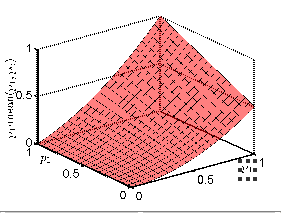
(a) MeanVec

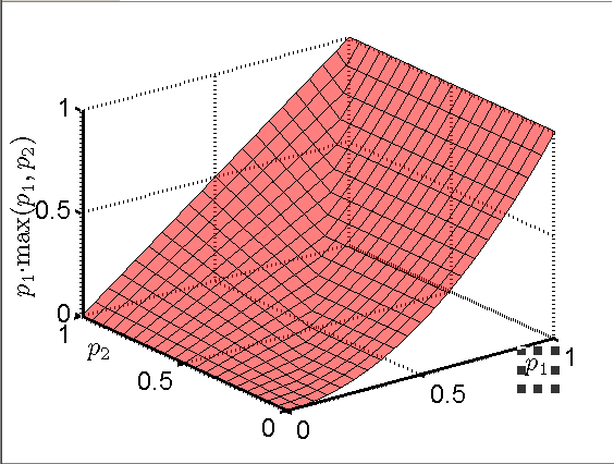
(b) MaxVec

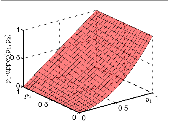
(c) UpperVec

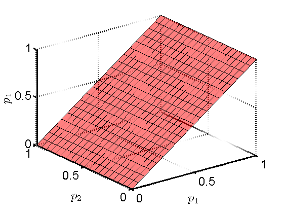
(d) Linear

Figure 1: Illustration of our pooling operators. Figures 1(a), 1(b), 1(c) and 1(d) show MeanVec, MaxVec, UpperVec and the linear case, respectively.

Figure 1 shows our summarizing operators. For the sake of clarity, we assume point-wise convolutions of some $\mathbf{h}^{(l-1)}_{u}$ with only two filters $\mathbf{w}_{1l}$ and $\mathbf{w}_{2l}$ which result in $p_{1}$ and $p_{2}$ proportional to correlation levels. The role of each pooling operator is explained below.

Figure 1(a) shows that MeanVec is a non-linear operator, however, as $p_{2}\!\rightarrow\!0$, even if $p_{1}\!\rightarrow\!1$, the final response $p_{1}\!\cdot\!\text{mean}\big{(}p_{1},\cdots,p_{2})$ drops to 0.5 which is an undesired effect as $p_{1}\!\rightarrow\!1$ indicates high confidence in filter $\mathbf{w}_{1l}$ being activated (correlated with the feature vector).

Figure 1(b) shows that MaxVec solves the above issue e.g., if $p_{1}\!\rightarrow\!1$, then $p_{1}\!\cdot\!\text{max}\big{(}p_{1},\cdots,p_{2})\!\rightarrow\!1$, which reflects the strong confidence in the activation of filter $\mathbf{w}_{1l}$. As $p_{1}\!<\!1$ and $p_{2}\!<\!1$, the activation of $\mathbf{w}_{1l}$ drops, as desired. Moreover, our confidence in activation depends on the probability of $p_{1}$ times the probability of at least one detection of among $p_{1}$ and $p_{2}$ being observed, which is proportional to $h^{\prime}_{1}\!\cdot\!\text{max}({\mathbf{h}^{\prime}})$. This mechanism propagates the most informative activations to the next layer while suppressing uninformative activations.

Notably, if $p_{2}\!=\!1$, MaxVec acts as a linear function w.r.t. $p_{1}$. This means the complexity of the signal is deemed low by GCN, due to the linear regime being selected. For $p_{2}\!<\!1$, MaxVec becomes non-linear. The smaller the value of $p_{2}$, the greater the convexity, which validates our claim that the Factorized Bilinear model acts as a low-rank modulator of level of non-linearity if paired with our MaxVec operator.

Figure 1(c) shows that UpperVec indeed is an upper bound of MaxVec, which gives it a nice probabilistic interpretation explained just below Eq. 8.

Figure 1(d) shows the ordinary case, where the point-wise convolution is not followed by pooling. Then, $p_{1}$ simply behaves linearly (as it is not modulated by $p_{2}$), and $p_{1}$ is as an upper bound of MaxVec (and other operators). Alas, the linear setting violates the depth efficiency of neural nets.

4.5 Complexity Analysis

The computation cost of MaxVec is $\mathcal{O}(k)$ only as running maximum along $k$ dimensional vector $\mathbf{W}_{l}\mathbf{h}^{(l-1)}_{u}$ needs to touch $k$ elements. Moreover, MeanVec costs also $\mathcal{O}(k)$. However, the cost of TopKVec is $\mathcal{O}(k^{\prime}+k\log(k))$ as the biggest cost is that incurred by the sorting function e.g., incremental sorting, but the standard practice is to provide the asymptotic cost which amounts to $\mathcal{O}(k^{\prime}+k\log(k^{\prime}))$. DiagVec cost is $\mathcal{O}(k)$. The above costs represent the only extra computational cost incurred by us compared with the vanilla GCN layer. As a result, our model has close-to-linear/linear complexity w.r.t. $k$. We provide the runtime with the GFB layers in the experiments section.

5 Experiments

In this section, we evaluate the proposed method on three experimental tasks. We (i) determine if our model achieves satisfactory results in text classification and brings advantages over Text GCN [34] (vanilla GCN for text classification), and (ii) show that the proposed method is more efficient than other billinear pooling methods in text classification. We also provide evaluations on the entity recognition/graph classification in our supplementary material.

5.1 Setting

Baselines.

We compare our method with state of-the-art text classification and embedding methods such as: TF-IDF + LR, CNN [7], LSTM [16], PV-DBOW [13], PV-DM [13], PTE [29], fastText [6], SWEM [25], LEAM [31], Graph-CNN [4], Text GCN [34], SGC [32] and GIN [33].

Architecture of GCN. We found that a two-layer GCN performs better than a one layer GCN for the task of text classification, whereas adding more layer did not improve the performance. The paper on Text GCN and approach [9] also note this. As input features fed into the first layer are simply an identity matrix, the high-order aggregation in such a case is meaningless. Thus, in our two-layered architecture, the first layer follows Eq. 1, and the second layer uses variants such as GFB, Factorized Bilinear Pooling (FBP), Compact Billinear Pooling (CBP) and Bilinear Pooling (BP), described in the method section.

5.2 Datasets

We ran our experiments on five widely used benchmark corpora including 20-Newsgroups (20NG), Ohsumed, R52 and R8 of Reuters 21578. We first preprocessed datasets by cleaning and tokenizing text [7]. We then removed stop words defined in NLTK6 and low frequency words appearing less than 5 times for 20NG, R8, R52 and Ohsumed.

Parameters.

We follow the setting of Text GCN [34] that includes experiments on four widely used benchmark corpora such as 20-Newsgroups (20NG), Ohsumed, R52 and R8 of Reuters 21578. For Text GCN and the proposed method, the embedding size of the first convolution layer is 200 and the window size is 20. We set the learning rate to 0.02, dropout rate to 0.5, the decay rate to 0, and $k=3$ for TopkVec. The 10% of training set is randomly selected for validation. Following [9], we trained our method and Text GCN for a maximum of 200 epochs using the Adam [8] optimizer, and we stop training if the validation loss does not decrease for 10 consecutive epochs. The text graph was built according to steps detailed in [34].

Table 1: Test accuracy on the document classification task. Some Abbreviations: Factorized Bilinear Pooling (FBP), Compact Bilinear Pooling (CBP), Square Root Pooling (Square root), Weighted Average Pooling (WAP). For Bilinear Pooling (BP), we did not report results as experiments would require 20 days of 10 GPUs to run (e.g., 863.1 seconds per epoch, 200 epochs, 10 runs for 20NG). However, on R8 (smallest dataset), Text GCN+BP yields 0.9682$\pm$0.0042.

Model	20NG	R8	R52	Ohsumed
TF-IDF + LR	0.8319 $\pm$ 0.0000	0.9374 $\pm$ 0.0000	0.8695 $\pm$ 0.0000	0.5466 $\pm$ 0.0000
CNN-rand	0.7693 $\pm$ 0.0061	0.9402 $\pm$ 0.0057	0.8537 $\pm$ 0.0047	0.4387 $\pm$ 0.0100
CNN-non-static	0.8215 $\pm$ 0.0052	0.9571 $\pm$ 0.0052	0.8759 $\pm$ 0.0048	0.5844 $\pm$ 0.0106
LSTM	0.6571 $\pm$ 0.0152	0.9368 $\pm$ 0.0082	0.8554 $\pm$ 0.0113	0.4113 $\pm$ 0.0117
PV-DBOW	0.7436 $\pm$ 0.0018	0.8587 $\pm$ 0.0010	0.7829 $\pm$ 0.0011	0.4665 $\pm$ 0.0019
PV-DM	0.5114 $\pm$ 0.0022	0.5207 $\pm$ 0.0004	0.4492 $\pm$ 0.0005	0.2950 $\pm$ 0.0007
PTE	0.7674 $\pm$ 0.0029	0.9669 $\pm$ 0.0013	0.9071 $\pm$ 0.0014	0.5358 $\pm$ 0.0029
fastText	0.7938 $\pm$ 0.0030	0.9613 $\pm$ 0.0021	0.9281 $\pm$ 0.0009	0.5770 $\pm$ 0.0049
SWEM	0.8516 $\pm$ 0.0029	0.9532 $\pm$ 0.0026	0.9294 $\pm$ 0.0024	0.6312 $\pm$ 0.0055
LEAM	0.8191 $\pm$ 0.0024	0.9331 $\pm$ 0.0024	0.9184 $\pm$ 0.0023	0.5858 $\pm$ 0.0079
Graph-CNN	0.8142 $\pm$ 0.0032	0.9699 $\pm$ 0.0012	0.9275 $\pm$ 0.0022	0.6386 $\pm$ 0.0053
Text GCN (WAP)	0.8597 $\pm$ 0.0014	0.9707 $\pm$ 0.0010	0.9356 $\pm$ 0.0018	0.6836 $\pm$ 0.0056
Text SGC (WAP)	0.8853 $\pm$ 0.0005	0.9723 $\pm$ 0.0002	0.9403 $\pm$ 0.0003	0.6853 $\pm$ 0.0003
Text GIN (WAP)	0.8414 $\pm$ 0.0084	0.9352 $\pm$ 0.0154	0.9314 $\pm$ 0.0074	0.6323 $\pm$ 0.0098
FBP (Eq.5)	0.8426 $\pm$ 0.0021	0.9659 $\pm$ 0.0045	0.9370 $\pm$ 0.0097,	0.6601 $\pm$ 0.0050
CBP	0.7789 $\pm$ 0.0078	0.9404 $\pm$ 0.0203	0.8638 $\pm$ 0.0900,	0.5986 $\pm$ 0.0098
Text GCN + Square root	0.8618 $\pm$ 0.0013	0.9700 $\pm$ 0.0011	0.9383 $\pm$ 0.0013	0.6915 $\pm$ 0.0029
GFBP+MeanVec	0.8657 $\pm$ 0.0018	0.9744 $\pm$ 0.0017	0.9424 $\pm$ 0.0009	0.6943 $\pm$ 0.0039
GFBP+DiagVec	0.8682 $\pm$ 0.0013	0.9767 $\pm$ 0.0011	0.9450 $\pm$ 0.0011	0.7164 $\pm$ 0.0023
GFBP+MaxVec	0.8718 $\pm$ 0.0017	0.9770 $\pm$ 0.0009	0.9448 $\pm$ 0.0016	0.7174 $\pm$ 0.0022
GFBP + TopKVec	0.8692 $\pm$ 0.0015	0.9756 $\pm$ 0.0024	0.9466 $\pm$ 0.0019,	0.7107 $\pm$ 0.0021

5.3 Results

Table 1 presents the test accuracy of each model. Our method significantly outperforms all other models which showcases the effectiveness of our method on long text datasets. We notice that for Ohsumed and R52, the improvements are relatively greater than on other datasets and thus we analyze these results in our supplementary material. We also provide other results based on variants of Text GCN with SGC [32] and GIN [33]. Note that SGC do not have hidden layer, thus the embedding of words and documents for 20NG are over 10000 size, which makes SGC gain advantage.

To showcase the effectiveness of our idea, we also provide comparisons to bilinear aggregation (e.g., Eq. 4), compact billinear pooling, and factorized bilinear pooling [14]. Because bilinear aggregation is extremely slow (about one month to finish evaluations on four datasets), we only provide a single result on R8, that is 0.9682$\pm$0.0042.

Speed Analysis

We show the runtime speed comparison of a two-layer GCN in Table 2. The test is performed on the GTX1080 GPU. From Table 2, we can see that all factorized methods (including FBP) are more efficient than bilinear pooling, which is two orders of magnitude slower compared to first-order methods. Compared with the vanilla text GCN, the proposed methods only slightly increase computation cost (20%-30%). The GFBP+DiagVec is the fastest while GFBP+MaxVec is marginally slower but provides overall best results. We also provide the speed of Compact Bilinear Pooling (CBP). Although CBP is just slightly slower than our method, its recognition performance is not competitive.

Table 2: Time cost per epoch during training on the document classification task (in seconds).

Model	20NG	R8	R52	Ohsumed
Text GCN	13.90	0.998	1.673	3.300
FBP (Eq.5)	15.63	1.242	2.317	3.907
CBP	23.09	1.664	2.531	4.913
BP (Eq.4)	863.1	111.6	126.4	261.8
GFBP+MeanVec	16.80	1.207	2.057	3.999
GFBP+DiagVec	14.98	1.143	2.097	3.608
GFBP+MaxVec	18.39	1.248	2.076	3.933
GFBP+TopKVec	23.34	2.032	8.707	6.607

Fast Convergence of GCN with Generalized Factorized Model.

Below, we compare the convergence of our Generalized Factorized Model against the Vanilla GCN. Fig. 2 demonstrates the number of epochs for each method till early stopping criterion is met (no further increase in the classification performance during validation). The GFBP+MeanVec and TopKVec converge much faster than other methods. The other two variants of GFBP are also competitive compared to the vanilla GCN, although for R52, they need few more epochs than the Text GCN. On other datasets, these variants still converge faster than the TextGCN. Compared with the Text GCN, the convergence of the proposed method is significantly faster as our method converges in less than 30 epochs (32 epochs on ohsumed dataset). At the same time, Text GCN runs until the 68 epoch (the early stopping condition). This trend is consistent on all four datasets. The faster convergence stems from the ability of our sumamrization operators to ‘pool’ features between channels (thus reducing degrees of freedom that stem from the correlation of features in different channels) [12].

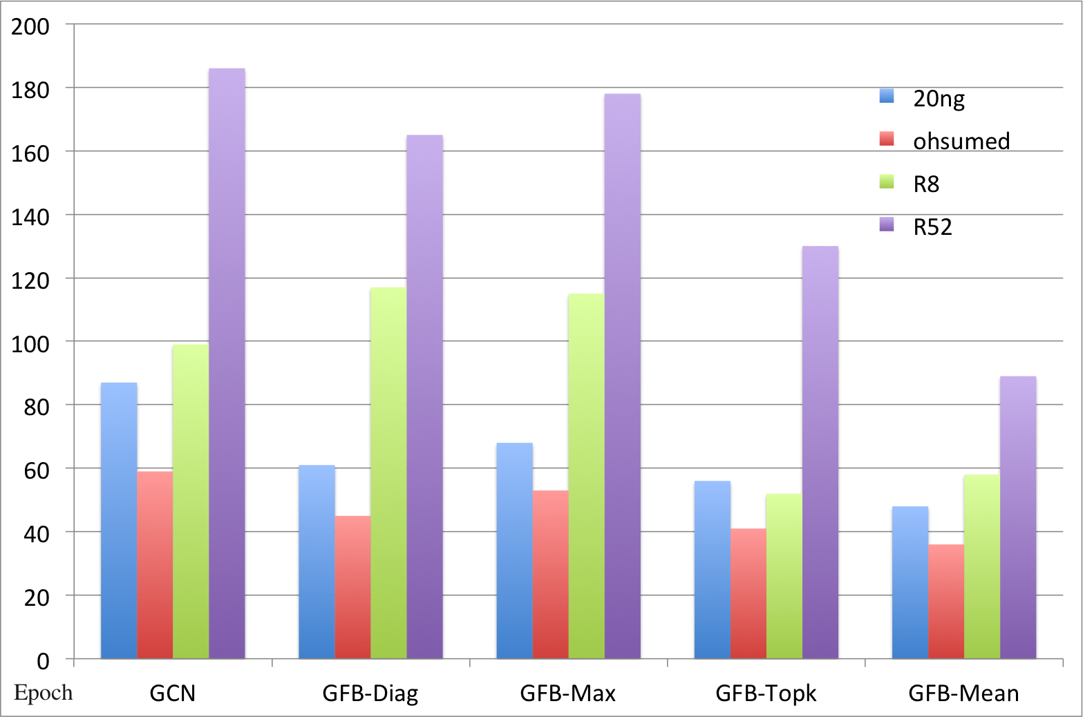
Figure 2: The number of epochs at which the early stopping criterion was met (proposed methods vs. the vanilla GCN).

6 Discussion and Conclusions

In this paper, we have proposed a novel neighbourhood aggregation scheme for GCNs and showcased results on the Text GCN. Instead of using first-order local average pooling, we have introduced a generalized factorized bilinear neighbourhood aggregation scheme with summarization operators that attain compactness on the par of first-order average pooling, exploit correlation between channels, and realize low-rank modulation of pooling to interpolate between linear activation (simple signals) and various levels of non-linear activations realized by our operator. Our supplementary material presents further results on text classification (different metrics), entity recognition and graph classification.

Appendix A Text Classification

A.1 Text Graph

To convert text classification into the node classification on graph, there are two relationships considered when forming graphs: (i) the relation between documents and words and (ii) the connection between words. For the first type of relations, we build edges among word nodes and document nodes based on the word occurrence in documents. The weight of the edge between a document node and a word node is the Term Frequency-Inverse Document Frequency [20] (TF-IDF) of the word in the document applied to build the Docs-words graph. For the second type of relations, we build edges in graph among word co-occurrences across the whole corpus. To utilize the global word co-occurrence information, we use a fixed-size sliding window on all documents in the corpus to gather co-occurrence statistics. Point-wise Mutual Information [2] (PMI), a popular measure for word associations, is used to calculate weights between two word nodes according to the following definition:

$$\text{PMI}(i,j)=\log\frac{p(i,j)}{p(i)p(j)}$$ (9)

where $p(i,j)=\frac{W(i,j)}{W}$, $p(i)=\frac{W(i)}{W}$. $W(i)$ is the number of sliding windows in a corpus that contain word $i$, $W(i,j)$ is the number of sliding windows that contain both word $i$ and word $j$, and $W$ is the total number of sliding windows in the corpus. A positive PMI value implies a high semantic correlation of words in a corpus, while a negative PMI value indicates little or no semantic correlation in the corpus. Therefore, we only add edges between word pairs with positive PMI values:

$$\mathbf{A}=\left[\begin{array}[]{c|c}\mathbf{W}_{1}&\mathbf{W}_{2}\\ \hline\cr\mathbf{W}_{2}^{\top}&\mathbf{I}\end{array}\right]$$

or

$$A_{ij}=\left\{\begin{aligned} \text{PMI}(i,j)&\quad\text{if }i,j~{}\text{are words, PMI}(i,j)>0,\\ \text{TF-IDF}_{ij}&\quad\text{if }i~{}\text{is document},j~{}\text{is word},\\ 1&\quad\text{if }i=j,\\ 0&\quad\text{otherwise}.\end{aligned}\right.$$ (10)

A.2 Relationship to Factorization Machines

Factorization Machine (FM) [21] is a popular predictor in machine learning and data mining, especially for very sparse data. Factorized Bilinear (FB) Model  [14] is much more general, which can be integrated into regular neural networks seamlessly for different kinds of tasks because it extends FM to multi-dimensions. In this way, a 2-way FM is a special case of our FB model. Our approach, Generalized Factorized Billinear Model, is more general and compact than the FM model e.g., we can modulate the level of non-linearity in the response. As an example, we can rewrite the transformation part with DiagVec as:

$$y=\mathbf{W}\mathbf{x}+\mathbf{F}\mathbf{x}\otimes(\mathbf{F}\mathbf{x})^{\top},\;\text{s.t. }\mathbf{F}=\lambda\mathbf{W},$$ (11)

where we suppress learning a new parameter matrix $\mathbf{F}$ for feature interactions. Instead of it, we only add a differentiable parameter $\lambda$ and a constraint as $\mathbf{F}=\lambda\mathbf{W}$. In the experiments, we demonstrate that our proposed method is more efficient and effective.

Table 3: The statistics of datasets.

Dataset	# Docs	# Training	# Test	# Words	# Nodes	# Classes	Average Length
20NG	18,846	11,314	7,532	42,757	61,603	20	221.26
R8	7,674	5,485	2,189	7,688	15,362	8	65.72
R52	9,100	6,532	2,568	8,892	17,992	52	69.82
Ohsumed	7,400	3,357	4,043	14,157	21,557	23	135.82

A.3 Datasets

We ran our experiments on five widely used benchmark corpora including 20-Newsgroups (20NG), Ohsumed, R52 and R8 of Reuters 21578.

The 20NG dataset1

(bydate version) contains 18,846 documents evenly categorized into 20 different categories. In total, 11,314 documents are in the training set and 7,532 documents are in the test set.

The Ohsumed corpus2, a part of the MEDLINE database, is a bibliographic database of important medical literature maintained by the National Library of Medicine. In this work, we used the 13,929 unique cardiovascular diseases abstracts in the first 20,000 abstracts of the year 1991. Each document in the set has one or more associated categories from the 23 disease categories. As we focus on single-label text classification, the documents belonging to multiple categories are excluded so that 7,400 documents belonging to only one category remain. 3,357 documents are in the training set and 4,043 documents are in the test set.

R52 and R8

(all-terms version) are two subsets of the Reuters 21578 dataset. R8 has 8 categories, and was split to 5,485 training and 2,189 test documents. R52 has 52 categories, and was split to 6,532 training and 2,568 test documents.

A.4 Data Imbalance

Our method outperforms the Text GCN in terms of accuracy. However, the definition of accuracy for multi-class tasks (a simple average) may disadvantage algorithms in presence of imbalanced domains. R52 is the most imbalanced datasets for which the number of samples in each category varies from 1 to 1083. Thus, we analyze results in terms of Macro-Precision, Macro-Recall and Macro-F1. The results in Table 4 show significant improvements in terms of macro-recall and macro-F1, which shows that our method can classify correctly samples belonging to categories with very limited training samples. We also obtain the similar result on Ohsumed (in Table. 5), where the number of samples in each category varies from 10 to 600, although the number of categories is below the number of categories of R52.

Table 4: Macro-Precision, Recall, F-1 Results on R52.

R52	Precision	Recall	F1
Text GCN	0.7561	0.6694	0.6864
GFB+MeanVec	0.7654	0.6864	0.7058
GFB+DiagVec	0.7662	0.6747	0.6925
GFB+MaxVec	0.7598	0.6845	0.6980
GFB+TopKVec	0.7741	0.6834	0.7008

Table 5: Macro-Precision, Recall, F-1 Results on Ohsumed.

Ohsumed	Precision	Recall	F1
Text GCN	0.6814	0.5913	0.6216
GFB+MeanVec	0.6606	0.6110	0.6255
GFB+DiagVec	0.6873	0.6336	0.6517
GFB+MaxVec	0.6938	0.6279	0.6510
GFB+TopKVec	0.6813	0.6256	0.6446

Appendix B Entity Classification

Below, we study the task of entity classification in a knowledge base. In order to infer, for example, the type of an entity (e.g., person or company), a successful model needs to reason about the relations with other entities that the main entity is involved in.

B.1 Extension of R-GCN to Generalized Factorized Bilinear R-GCN (GFB-R-GCN)

According to the [24], the R-GCN update of an entity or node denoted by $v_{i}$ in a relational (directed and labeled) multi-graph is given as:

$$h_{i}^{(l+1)}=\sigma\left(\sum_{r\in\mathcal{R}}\sum_{j\in\tilde{\mathcal{N}}_{i}^{r}}\frac{1}{c_{i,r}}\mathbf{W}_{r}^{(l)}\mathbf{h}_{j}^{(l)}+\mathbf{W}_{0}^{(l)}\mathbf{h}_{i}^{(l)}\right),$$ (12)

where $\tilde{\mathcal{N}}_{i}^{r}$ denotes the set of neighbor indices of node $i$ under relation $r\in R$, $c_{i,r}$ is a problem-specific normalization constant that can either be learned or chosen in advance e.g., $c_{i,r}=\left|\mathcal{N}_{i}^{r}\right|$.

Our Generalized Factorized Bilinear model with the summarization function, termed as GFB-R-GCN, becomes:

$$\mathbf{h}^{(l)}_{v}=\sigma\Big{(}\sum_{r\in\mathcal{R}}\sum_{j\in\tilde{\mathcal{N}}_{i}^{r}}\mathbf{W}_{r}^{(l)}\mathbf{h}^{(l-1)}_{j}+\lambda_{l}\textbf{GenVec}(\mathbf{M})\Big{)},$$ (13)

where we set $\mathbf{M}\!=\!\mathbf{W}_{r}^{(l)}\mathbf{h}^{(l-1)}_{j}{\mathbf{h}^{(l-1)}_{j}}^{\top}\mathbf{W}_{r}^{(l)}\top$, and we choose a desired definition of $g(\cdot)$ according to the main submission e.g., we use the MeanVec operator.

Datasets.

We evaluate our model on four datasets in Resource Description Framework (RDF) format [22]: AIFB, MUTAG, BGS, and AM. Relations in these datasets need not necessarily encode directed subject-object relations, but are also used to encode the presence or absence of a specific feature for a given entity. For each dataset, the targets to be classified are properties of a group of entities represented as nodes. For a more detailed description of the datasets the reader is referred to [22]. We remove relations that were used to create entity labels: employes and affiliation for AIFB, isMutagenic for MUTAG, hasLithogenesis for BGS, and objectCategory and material for AM.

Table 6: Entity classification results (accuracy % averaged over 10 runs) for a feature-based baseline (see the main text for details), WL RDF2Vec , R-GCN and GFB-R-GCN . Test performance is reported on the train/test set splits provided by R-GCN.

Model	AIFB	MUTAG	BGS	AM
Feat	55.55	77.94	72.41	66.66
WL	80.55	80.88	86.20	87.37
RDF2Vec	88.88	67.20	87.24	88.33
R-GCN	95.83	73.23	83.10	89.29
GFB-R-GCN	97.22	77.94	89.66	90.40

Table 7: Results for the problem of graph classification.

	MUTAG	PROTEINS	IMDB-Binary	Redit-Binary	COLLAB
GCN	74.6 $\pm$ 7.7	73.1 $\pm$ 3.8	72.6 $\pm$ 4.5	89.3 $\pm$ 3.3	80.6 $\pm$ 2.1
GraphSage	74.9 $\pm$ 8.7	73.8 $\pm$ 3.6	72.4 $\pm$ 3.6	89.1 $\pm$ 1.9	79.7 $\pm$ 1.7
GFB-GCN	83.5 $\pm$ 4.7	74.2 $\pm$ 3.9	74.4 $\pm$ 5.4	90.6 $\pm$ 2.6	80.0 $\pm$ 2.3
GFB-GraphSage	81.4 $\pm$ 7.5	74.4 $\pm$ 4.4	73.9 $\pm$ 4.9	88.9 $\pm$ 2.2	79.5 $\pm$ 2.3

Baselines.

As a baseline for our experiments, we compare against recent state-of-the-art classification results from RDF2Vec embeddings [23], Weisfeiler-Lehman kernels (WL) [26, 3], and hand-designed feature extractors (Feat) [18]. Feat assembles a feature vector from the in- and out-degree (per relation) of every labeled entity. RDF2Vec extracts walks on labeled graphs which are then processed using the Skipgram [17] model to generate entity embeddings, used for subsequent classification. All entity classification experiments were performed on a CPU machine with 64GB of memory.

Results.

Results in Table 6 are reported on the train/test benchmark splits from [22]. We further set aside 20% of the training set as a validation set for hyperparameter tuning. For R-GCN, we report performance of a 2-layer model with 16 hidden units (10 for AM). We trained with Adam [8] for 50 epochs using a learning rate of 0.01. The normalization constant is chosen as $c_{i,r}=\left|\mathcal{N}_{i}^{r}\right|$. and hyperparameter choices are provided in the supplementary material. The GFB-GCN employ the MeanVec in the aggregator function.

Appendix C Graph Classification

In Table 7, we report the average accuracy of 10-fold cross validation on a number of common benchmark datasets. We randomly sample a training fold to serve as a validation set. We only make use of discrete node features. In case they are not given, we use one-hot encodings of node degrees as feature input. For all experiments, we use the global mean operator to obtain graph-level outputs. For evaluating the Generalized Bilinear Pooling, we use the GraphSAGE and GCN as our baseline. For each dataset, we tune (1) the number of hidden units $\in\{16,32,64,128\}$ and (2) the number of layers $\in\{1,2,3,4,5\}$ with respect to the validation set. Our GFB based methods use DiagVec in the aggregation function.

References

- [1] Charu C Aggarwal and ChengXiang Zhai. A survey of text classification algorithms. In Mining text data, pages 163–222. Springer, 2012.
- [2] Kenneth Ward Church and Patrick Hanks. Word association norms, mutual information, and lexicography. Computational linguistics, 16(1):22–29, 1990.
- [3] Gerben Klaas Dirk De Vries and Steven De Rooij. Substructure counting graph kernels for machine learning from rdf data. Journal of Web Semantics, 35:71–84, 2015.
- [4] Michaël Defferrard, Xavier Bresson, and Pierre Vandergheynst. Convolutional neural networks on graphs with fast localized spectral filtering. In Advances in neural information processing systems, pages 3844–3852, 2016.
- [5] Fuli Feng, Xiangnan He, Hanwang Zhang, and Tat-Seng Chua. Cross-gcn: Enhancing graph convolutional network with k-order feature interactions. IEEE Transactions on Knowledge and Data Engineering, 2021.
- [6] Armand Joulin, Edouard Grave, Piotr Bojanowski, and Tomas Mikolov. Bag of tricks for efficient text classification. arXiv preprint arXiv:1607.01759, 2016.
- [7] Yoon Kim. Convolutional neural networks for sentence classification. arXiv preprint arXiv:1408.5882, 2014.
- [8] Diederik P Kingma and Jimmy Ba. Adam: A method for stochastic optimization. arXiv preprint arXiv:1412.6980, 2014.
- [9] Thomas N Kipf and Max Welling. Semi-supervised classification with graph convolutional networks. arXiv preprint arXiv:1609.02907, 2016.
- [10] Piotr Koniusz, Fei Yan, Philippe-Henri Gosselin, and Krystian Mikolajczyk. Higher-order occurrence pooling for bags-of-words: Visual concept detection. IEEE Transactions on Pattern Analysis and Machine Intelligence, 39:1–1, 03 2016.
- [11] Piotr Koniusz and Hongguang Zhang. Power normalizations in fine-grained image, few-shot image and graph classification. In IEEE Transactions on Pattern Analysis and Machine Intelligence. IEEE, 2020.
- [12] Piotr Koniusz, Hongguang Zhang, and Fatih Porikli. A deeper look at power normalizations. In Proceedings of the IEEE Conference on Computer Vision and Pattern Recognition, pages 5774–5783, 2018.
- [13] Quoc Le and Tomas Mikolov. Distributed representations of sentences and documents. In International conference on machine learning, pages 1188–1196, 2014.
- [14] Yanghao Li, Naiyan Wang, Jiaying Liu, and Xiaodi Hou. Factorized bilinear models for image recognition. In Proceedings of the IEEE International Conference on Computer Vision, pages 2079–2087, 2017.
- [15] Tsung-Yu Lin, Aruni RoyChowdhury, and Subhransu Maji. Bilinear cnn models for fine-grained visual recognition. In Proceedings of the IEEE international conference on computer vision, pages 1449–1457, 2015.
- [16] Pengfei Liu, Xipeng Qiu, and Xuanjing Huang. Recurrent neural network for text classification with multi-task learning. arXiv preprint arXiv:1605.05101, 2016.
- [17] Tomas Mikolov, Ilya Sutskever, Kai Chen, Greg S Corrado, and Jeff Dean. Distributed representations of words and phrases and their compositionality. In Advances in neural information processing systems, pages 3111–3119, 2013.
- [18] Heiko Paulheim and Johannes Fümkranz. Unsupervised generation of data mining features from linked open data. In Proceedings of the 2nd international conference on web intelligence, mining and semantics, pages 1–12.
- [19] Hao Peng, Jianxin Li, Yu He, Yaopeng Liu, Mengjiao Bao, Lihong Wang, Yangqiu Song, and Qiang Yang. Large-scale hierarchical text classification with recursively regularized deep graph-cnn. In Proceedings of the 2018 World Wide Web Conference, pages 1063–1072, 2018.
- [20] Anand Rajaraman and Jeffrey David Ullman. Mining of massive datasets. Cambridge University Press, 2011.
- [21] Steffen Rendle. Factorization machines with libfm. ACM Transactions on Intelligent Systems and Technology (TIST), 3(3):1–22, 2012.
- [22] Petar Ristoski, Gerben Klaas Dirk De Vries, and Heiko Paulheim. A collection of benchmark datasets for systematic evaluations of machine learning on the semantic web. In International Semantic Web Conference, pages 186–194. Springer, 2016.
- [23] Petar Ristoski and Heiko Paulheim. Rdf2vec: Rdf graph embeddings for data mining. In International Semantic Web Conference, pages 498–514. Springer, 2016.
- [24] Michael Schlichtkrull, Thomas N Kipf, Peter Bloem, Rianne Van Den Berg, Ivan Titov, and Max Welling. Modeling relational data with graph convolutional networks. In European Semantic Web Conference, pages 593–607. Springer, 2018.
- [25] Dinghan Shen, Guoyin Wang, Wenlin Wang, Martin Renqiang Min, Qinliang Su, Yizhe Zhang, Chunyuan Li, Ricardo Henao, and Lawrence Carin. Baseline needs more love: On simple word-embedding-based models and associated pooling mechanisms. arXiv preprint arXiv:1805.09843, 2018.
- [26] Nino Shervashidze, Pascal Schweitzer, Erik Jan Van Leeuwen, Kurt Mehlhorn, and Karsten M Borgwardt. Weisfeiler-lehman graph kernels. Journal of Machine Learning Research, 12(9), 2011.
- [27] Ke Sun, Piotr Koniusz, and Zhen Wang. Fisher-bures adversary graph convolutional networks. In Ryan P. Adams and Vibhav Gogate, editors, Proceedings of The 35th Uncertainty in Artificial Intelligence Conference, volume 115 of Proceedings of Machine Learning Research, pages 465–475. PMLR, 22–25 Jul 2020.
- [28] Kai Sheng Tai, Richard Socher, and Christopher D Manning. Improved semantic representations from tree-structured long short-term memory networks. arXiv preprint arXiv:1503.00075, 2015.
- [29] Jian Tang, Meng Qu, and Qiaozhu Mei. Pte: Predictive text embedding through large-scale heterogeneous text networks. In Proceedings of the 21th ACM SIGKDD International Conference on Knowledge Discovery and Data Mining, pages 1165–1174, 2015.
- [30] O. Tuzel, F. Porikli, and P. Meer. Region covariance: A fast descriptor for detection and classification. ECCV, 2006.
- [31] Guoyin Wang, Chunyuan Li, Wenlin Wang, Yizhe Zhang, Dinghan Shen, Xinyuan Zhang, Ricardo Henao, and Lawrence Carin. Joint embedding of words and labels for text classification. arXiv preprint arXiv:1805.04174, 2018.
- [32] Felix Wu, Amauri Souza, Tianyi Zhang, Christopher Fifty, Tao Yu, and Kilian Weinberger. Simplifying graph convolutional networks. In International Conference on Machine Learning, pages 6861–6871, 2019.
- [33] Keyulu Xu, Weihua Hu, Jure Leskovec, and Stefanie Jegelka. How powerful are graph neural networks? In International Conference on Learning Representations, 2018.
- [34] Liang Yao, Chengsheng Mao, and Yuan Luo. Graph convolutional networks for text classification. In Proceedings of the AAAI Conference on Artificial Intelligence, volume 33, pages 7370–7377, 2019.
- [35] Xiang Zhang, Junbo Zhao, and Yann LeCun. Character-level convolutional networks for text classification. In Advances in neural information processing systems, pages 649–657, 2015.
- [36] Yufeng Zhang, Xueli Yu, Zeyu Cui, Shu Wu, Zhongzhen Wen, and Liang Wang. Every document owns its structure: Inductive text classification via graph neural networks. arXiv preprint arXiv:2004.13826, 2020.
- [37] Jie Zhou, Ganqu Cui, Zhengyan Zhang, Cheng Yang, Zhiyuan Liu, Lifeng Wang, Changcheng Li, and Maosong Sun. Graph neural networks: A review of methods and applications. arXiv preprint arXiv:1812.08434, 2018.
- [38] Hao Zhu and Piotr Koniusz. Simple spectral graph convolution. In International Conference on Learning Representations, 2021.
- [39] Hongmin Zhu, Fuli Feng, Xiangnan He, Xiang Wang, Yan Li, Kai Zheng, and Yongdong Zhang. Bilinear graph neural network with neighbor interactions. arXiv preprint arXiv:2002.03575, 2020.