Clinical Utility of the Automatic Phenotype Annotation in Unstructured Clinical Notes: ICU Use Cases

Jingqing Zhang Data Science Institute, Imperial College London, London, SW7 2AZ, UK Pangaea Data Limited, UK, USA These authors contributed equally to this work. Luis Bolanos Pangaea Data Limited, UK, USA These authors contributed equally to this work. Ashwani Tanwar Pangaea Data Limited, UK, USA These authors contributed equally to this work. Julia Ive Department of Computing, Imperial College London, London, SW7 2AZ, UK Queen Mary University of London, London, E1 4NS, UK Vibhor Gupta Pangaea Data Limited, UK, USA Yike Guo Data Science Institute, Imperial College London, London, SW7 2AZ, UK Hong Kong Baptist University, Hong Kong SAR, China Pangaea Data Limited, UK, USA Correspondence to: y.guo@imperial.ac.uk

Abstract

Objective

Clinical notes contain information not present elsewhere, including drug response and symptoms, all of which are highly important when predicting key outcomes in acute care patients. We propose the automatic annotation of phenotypes from clinical notes as a method to capture essential information, which is complementary to typically used vital signs and laboratory test results, to predict outcomes in the Intensive Care Unit (ICU).

Methods

We develop a novel phenotype annotation model to annotate phenotypic features of patients which are then used as input features of predictive models to predict ICU patient outcomes. We demonstrate and validate our approach conducting experiments on three ICU prediction tasks including in-hospital mortality, physiological decompensation and length of stay for over 24,000 patients by using MIMIC-III dataset.

Results

The predictive models incorporating phenotypic information achieve 0.845 (AUC-ROC) to predict in-hospital mortality, 0.839 (AUC-ROC) for physiological decompensation and 0.430 (Kappa) for length of stay, all of which consistently outperform the baseline models leveraging only vital signs and laboratory test results. Moreover, we conduct a thorough interpretability study, showing that phenotypes provide valuable insights at the patient and cohort levels.

Conclusion

The proposed approach demonstrates phenotypic information complements traditionally used vital signs and laboratory test results, improving significantly forecast of outcomes in the ICU.

Summary

What is already known?

•

Previous works have demonstrated good performance for prediction of outcomes in the Intensive Care Unit (ICU) using bedside measurements and laboratory test results
•

Contextual embeddings from recent Transformer-based Natural Language Processing models have enabled a more accurate detection of medical concepts

What does this paper add?

•

This paper introduces a new methodology to incorporate contextualized phenotypic features from clinical text and their persistency into the modelling of ICU time-series prediction tasks
•

We conduct an interpretability study, illustrating why and how phenotypic features are highly relevant for ICU outcomes prediction

Introduction

The accumulation of healthcare data today has reached unprecedented levels: NHS datasets alone record billions of patient interactions every year [1]. In particular, due to the close monitoring of patients in an Intensive Care Unit (ICU), a wealth of data is generated for each patient[2], with some information being recorded every minute.

In the typical setting, an Electronic Health Record (EHR) contains two types of information, which are structured (e.g. blood tests, temperature, lab results) and unstructured information (e.g. nursing notes, radiology reports, discharge summaries), with the latter composing the biggest part (typically, up to 80% [3]). Both types of information are valuable for the ICU monitoring. The majority of recent research [4, 5, 6] relies though on more straightforward structured information, typically being laboratory test results and vital signs.

Among the unstructured data, the phenotype¹¹1In the medical text, the word “phenotype” refers to deviations from normal morphology, physiology, or behaviour [7]. has been received the least attention for the ICU monitoring [8]. This is mainly due to the challenge to extract the phenotypic information expressed by a variety of contextual synonyms. For example, such a phenotype as Hypotension can be expressed in text as “drop in blood pressure” and “BP of 79/48”. However, the phenotypes are crucial for understanding disease diagnosis, identifying important disease-specific information, stratifying patients and identifying novel disease subtypes [9].

Our work thoroughly investigates the value of phenotypic information as extracted from text for ICU monitoring. We automatically extract mentions of phenotypes from clinical text using a self-supervised methodology with recent advancements in clinical NLP - contextualized word embeddings [10] that are particularly helpful for the detection of contextual synonyms. We extract those mentions for over 15,000 phenotype concepts of the Human Phenotype Ontology (HPO) [11]. We enrich the phenotypic features extracted in this manner with the information coming from the structured data (i.e., bedside measurements and laboratory test results). To provide interpretation into our results we use SHAP values[12].

We benchmark our approach on the following three mainstream ICU tasks following the practice [4] for comparison: length of stay, in-hospital mortality and physiological decompensation.

Our main contributions are: (i) approach to incorporate phenotypic features into the modelling of ICU time-series prediction tasks; (ii) investigation of the importance of the phenotypic features in combination with structured information for the prediction of patient course at micro (individual patient) and macro (cohort) levels; (iii) thorough interpretability study demonstrating the importance of phenotypic features and structured features for the ICU cases; (iv) demonstration of the utility of automatic phenotyping for ICU use cases.

Methodology

0.1 Data preprocessing

In this study, we use the publicly available ICU database MIMIC-III [13] and follow the common practice [4] to define the three ICU tasks, data collection and data preprocessing. We formulate the in-hospital mortality problem as a binary classification at 48 hours after admission, in which the label indicates whether the patient dies before discharge. We formulate the problem of physiological decompensation as a binary classification, in which the target label corresponds to whether the patient will die in the next 24 hours. We cast the length of stay (LOS) prediction task as a multi-class classification problem, where the labels correspond to the remaining length of stay. Possible values are divided into 10 bins, one for the stays of less than a day, 7 bins for each day of the first week, another bin for the stays of more than a week but less than two, and the final bin for stays of more than two weeks.

For data collection, we use both structured data (e.g. bedside measurements) and unstructured data (e.g. clinical notes) following the filtering criteria [4] for the patients, admissions and ICU stays in all three tasks. In addition, we discard all the ICU episodes in which a clinical note is not recorded. This reduces our train and test data as compared to the benchmark [4], so we recalculate the baseline scores using their code on our new test set for fair comparison. Overall, there are over 24,000 patients in total and the exact numbers of patients, ICU episodes and timesteps per task are reported in Table A1. Mortality rate across all patients is 13.12% and decompensation rate across all timesteps is 2.01%. Most patients stay in ICU less than 7 days, and the distribution of ICU stays per LOS class is presented in detail in Table A2.

For data preprocessing of structured data, we follow the steps²²2Accessed in November 2021: https://github.com/YerevaNN/mimic3-benchmarks to collect 17 clinical features (i.e., capillary refill rate, diastolic blood pressure, fraction inspired oxygen, Glasgow coma scale eye opening, Glasgow coma scale motor response, Glasgow coma scale verbal response, Glasgow coma scale total, glucose, heart rate, height, mean blood pressure, oxygen saturation, respiratory rate, systolic blood pressure, temperature, weight, and pH). For data preprocessing of unstructured data, we collect all clinical notes including nursing notes, physician notes and discharge summaries at all timesteps during ICU stays and we observe there is high data sparsity as clinical notes are recorded roughly every 12 hours. The processed structured data and unstructured data are then used as inputs to our approach.

Algorithm development and analysis

The proposed approach consists of two steps. The first step is to collect clinical features (more specifically, phenotypic features, standardised by Human Phenotype Ontology (HPO) [11]) from unstructured data by using Natural Language Processing (NLP) algorithms. The second step is to combine the phenotypic features from unstructured data and the 17 clinical features from structured data as input features for machine learning classifiers to predict in-hospital mortality, physiological decompensation and LOS in separate.

First, to extract phenotypes from free-text clinical notes, we develop a state-of-the-art phenotyping model, which leverages contextualized word embeddings and data augmentation techniques (paraphrasing and synthetic text generation) to capture names, synonyms, abbreviations and, more importantly, contextual synonyms of phenotypes. For example, “drop in blood pressure” and “BP of 79/48” are both contextual synonyms of Hypotension (HP:0002615). As a result of the contextual detection of phenotype, the phenotyping model demonstrates superior performance than alternative phenotyping algorithms. We refer the readers to the work [14] for methodological details. For comparison, we also use alternative phenotyping methods including ClinicalBERT [10] (fine-tuned for phenotyping) and NCR [15]. NCR uses a convolutional neural network (CNN) to assign similarity scores to HPO concepts of phrases encoded by using pre-trained non-contextualized word embeddings.

Second, the phenotypic features are combined with structured clinical features together as input features to machine learning classifiers for prediction of the three ICU tasks. We use standard machine learning classifiers: Random Forest (RF) [16], and Long Short-Term Memory Network (LSTM) [17] for prediction. We distinguish the phenotypic features between persistent and transient ones to reduce feature sparsity. More precisely, if a phenotype is clinically deemed likely to last an entire admission in the vast majority of typical cases (e.g., tuberculosis, cancer), it is marked as ‘persistent’. In contrast, if the phenotype can be acquired or improved during an ICU stay, such as pain, fever, cough, it is marked as ‘transient’. We make transient and persistent phenotypes present from the moment it appears until a new clinical note appears, and until the end of the ICU stay, respectively. We find this beneficial and will discuss it in Section Phenotype persistency. We also address data sparsity by aggregating HPO terms into their parents (according to the HPO hierarchy).

Evaluation Metrics

To compare with the previous study [4], we use Area Under the Curve of Receiver Operating Characteristic (AUC-ROC) [18] and Area Under the Curve of Precision-Recall (AUC-PR) for In-Hospital Mortality and Physiological Decompensation tasks. We primarily rely on AUC-ROC for statistical analysis as it is threshold independent and used by the benchmark [4] as the primary metric. For the LOS task, we use Cohen’s Kappa [19] and Mean Absolute Deviation [20] (MAD) with primarily relying on the Kappa scores for statistical analysis.

Model evaluation and statistical analysis

We use a train-test split based on the benchmark[4], but exclude patients without clinical notes, resulting in 21,346 and 3,824 patients for train and test set, respectively. Further, we perform 4-fold cross validation on the training set. All splits are deterministic, so that all the classifiers with different data settings are trained and evaluated with the same subsets of data. We use the bootstrap resampling following the benchmark for statistical analysis of the scores. To compute confidence intervals on the test set we resample it 1,000 times for length of stay and decompensation, and 10,000 times for in-hospital mortality task. Then, we compute the scores on the resampled data to calculate 95% confidence intervals.

To provide interpretability and insights into model predictions, we use SHAP values[12], the implementation details of which are explained more in Appendix Shapley Values. The SHAP values are typically used to explain black box models, and allow us to quantify the importance of a feature and whether it impacts positively or negatively the outcome.

Results

Phenotyping

Across all three tasks, ClinicalBERT finds 664 phenotypes, NCR finds 1,441 phenotypes, and our methodology finds 1,446, in average. 30% of these phenotypes are persistent (on average across tasks).

Quantitative results

In general, we investigate the performance of two classifiers: Random Forest (RF) and LSTM. For each of them we investigate the following set of features: structured features only (S) and structured features enriched with phenotypic features coming from one of the three phenotype annotators (ClinicalBERT, NCR, ours).

The main results are presented in Table 1 and the results from statistical tests are presented in Table A4. Overall, they show that phenotypic information complements positively the structured information to improve performance on all tasks. The improvements with our phenotyping model are statistically significant across all tasks compared against using structured features only or alternative phenotyping algorithms, except for In-Hospital Mortality with RF.

This is explained by the fact that phenotypes carry highly valuable information, including response to therapy, development of complication, comorbidities and unmeasured indicators of illness severity, all of which are fundamental to correctly estimate the LOS and mortality risk of a patient [21, 22].

Classification Model	Features Design	AUC-ROC $\uparrow$	AUC-PR $\uparrow$
SAPS-II	-	0.756	0.312
APACHE-III	-	0.733	0.308
Random Forest	S	0.800 (0.775, 0.824)	0.339 (0.286, 0.395)
	S + NCR	0.828 (0.802, 0.853)	0.467 (0.404, 0.529)
	S + CB	0.812 (0.787, 0.838)	0.403 (0.345, 0.463)
	S + Ours	0.845 (0.826, 0.873)	0.462 (0.404, 0.524)
LSTM	S [4]	0.825	0.410
	S	0.826 (0.801, 0.848)	0.391 (0.334, 0.452)
	S + NCR	0.841 (0.818, 0.864)	0.453 (0.393, 0.513)
	S + CB	0.826 (0.802, 0.849)	0.414 (0.355, 0.476)
	S + Ours	0.845 (0.823, 0.868)	0.464 (0.405, 0.523)

(a) In-hospital mortality

Classification Model	Features Design	AUC-ROC $\uparrow$	AUC-PR $\uparrow$
Random Forest	S	0.826 (0.821, 0.831)	0.130 (0.123, 0.138)
	S + NCR	0.825 (0.821, 0.830)	0.124 (0.118, 0.131)
	S + CB	0.826 (0.821, 0.830)	0.125 (0.118, 0.132)
	S + Ours	0.845 (0.840, 0.850)	0.180 (0.171, 0.190)
LSTM	S [4]	0.809	0.125
	S	0.824 (0.819, 0.829)	0.126 (0.119, 0.133)
	S + NCR	0.834 (0.829, 0.839)	0.134 (0.127, 0.142)
	S + CB	0.833 (0.828, 0.838)	0.114 (0.108, 0.119)
	S + Ours	0.839 (0.834, 0.844)	0.145 (0.138, 0.153)

(b) Physiological decompensation

Classification Model	Features Design	Kappa $\uparrow$	MAD $\downarrow$
Random Forest	S	0.390 (0.388, 0.392)	136.8 (136.2, 137.4)
	S + NCR	0.390 (0.388, 0.392)	142.5 (141.9, 143.1)
	S + CB	0.376 (0.374, 0.379)	144.3 (143.7, 144.9)
	S + Ours	0.420 (0.418, 0.422)	110.3 (109.3, 111.3)
LSTM	S [4]	0.395	126.7
	S	0.380 (0.377, 0.382)	157.0 (156.3, 157.6)
	S + NCR	0.406 (0.404, 0.408)	123.3 (122.8, 123.9)
	S + CB	0.388 (0.386, 0.390)	120.1 (119.6, 120.6)
	S + Ours	0.430 (0.427, 0.432)	116.7 (116.1, 117.2)

Table 1: Results for (a) In-Hospital Mortality, (b) Physiological Decompensation, and (c) Length of Stay. Test set scores are shown with 95% confidence intervals in brackets if applicable. The best score for each classifier is highlighted in bold. The first row of LSTM refers to scores reported in previous literature, while the second row regards scores reproduce in this study with a comparable cohort. Here, S refers to Structured, NCR to Neural Concept Recognizer[15], CB to ClinicalBERT, and Ours to our phenotyping model.

Discussion

While we conclude that phenotypic information provides useful information to correctly conduct the three ICU tasks, decision support systems in the healthcare domain should be reliable, interpretable and robust. Therefore, we accompany the above results with a thorough study on interpretability, providing explanations both at the patient and cohort levels for the observed predictions, and an assessment of robustness by studying performances across disease-specific sub-cohorts.

Phenotype persistency

We find it beneficial to propagate phenotypes forwards in time. More precisely, each phenotypes is marked by one human clinical expert based on whether it would typically persist throughout an entire ICU stay or not. Consequently, transient (e.g., fever, cough, dyspnea) and persistent (e.g., diabetes, cancer) phenotypes are propagated until the appearance of a new clinical note or the end of the ICU stay, respectively. We perform an ablation study and observe the phenotype propagation is more beneficial to Random Forest (RF) than LSTM. The RF models with phenotype propagation achieve 4.6% higher AUC-ROC for in-hospital mortality, 2.5% higher AUC-ROC for decompensation and 3.4% higher Kappa for LOS than RF without phenotype propagation. However, the LSTM models with phenotype propagation achieve 1.4% higher AUC-ROC for in-hospital mortality, comparable results for decompensation and 1.1% lower Kappa for LOS. We hypothesise this is because LSTM by design can better capture temporal relationship given a large amount of data to learn from. The full results can be found in Table A6. We believe further investigation focused on learning persistency of phenotypes would be beneficial, not only to boost prediction accuracy, but also to provide insights about temporal duration of phenotypes in the ICU.

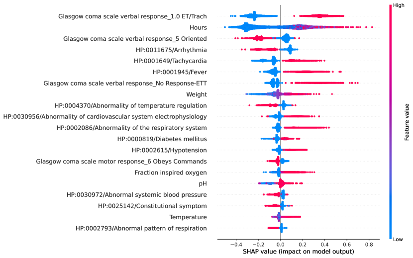
Phenotype importance

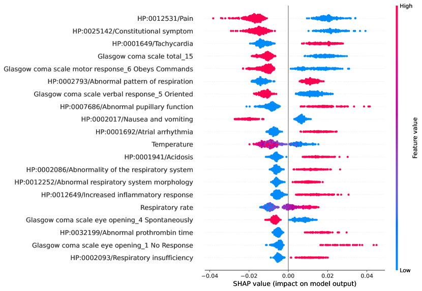
To further understand the contribution of phenotypic features to the prediction performance, we have studied the most important features with the help of SHAP values[12]. This analysis and all involving SHAP values are conducted on the Random Forest (RF) models. An illustration of our investigation is in Figure 1, where we present the top predicting features for in-hospital mortality and physiological decompensation. It confirms that phenotypic features are particularly helpful for the in-hospital mortality prediction, given that 13 out of the 20 most important features are phenotypes. This is explained by the fact that forecasts need to rely on information that is able to provide insights accurately into the long-term future.

Contrary to bedside measurements which may not correlate well with future outcomes due to their dynamic nature, phenotypes are highly informative given that they capture, for instance, comorbidities, which are essential for predicting mortality [22]. Furthermore, another study [23] including 230,000 ICU patients found that combining the comorbidities with acute physiological measurements yielded the best results, outperforming all mortality scores (APACHE-II, SAPS-II).

Unexpectedly and interestingly, the top ranking feature for mortality prediction is whether the patient experiences pain or not. We observe also that the second top ranking feature is Constitutional symptom (HP:0025142). Noting this is actually the resulting phenotype after aggregating all of its children, this phenotype should be interpreted not as a textual mention in the patient’s EHR of the broad term, but rather as a mention of any of its children (most notably generalized pain). Consequently, the second top feature again highlights the importance of pain.

Although not decisive, there is some initial evidence corroborating the fact that pain management improves outcomes in the ICU [24]. However, pain could also be interpreted as a proxy for establishing a high level of consciousness, which has been correlated with better outcomes in the ICU [25].

The other top ranking phenotypes, such as atrial arrhythmia, and nausea and vomiting, cover most of the body systems (i.e., heart, lungs, GI tract, central nervous system, coagulation, infection, kidneys) which are typically assessed through clinically validated scores e.g., APACHE, SAPS.

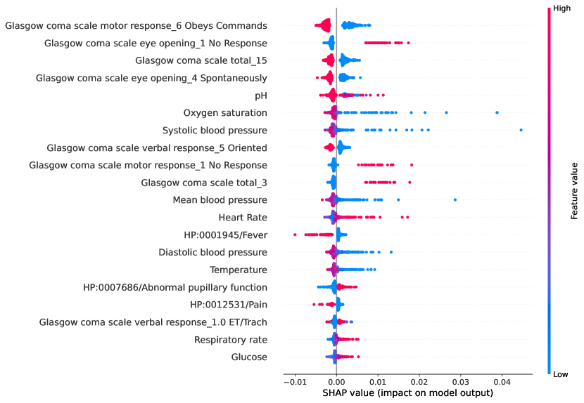
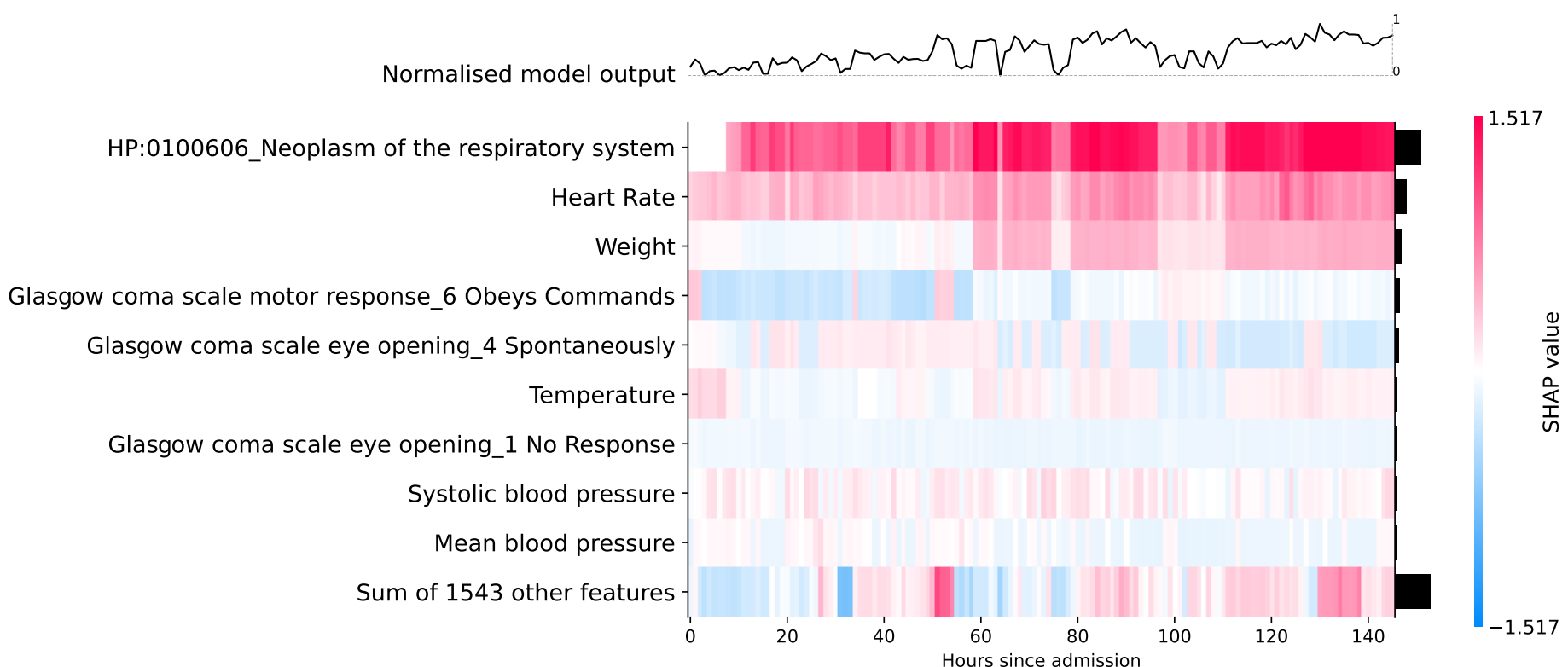
Refer to caption — (a) In-Hospital Mortality

Our study also showed that though phenotypic features are not as important for decompensation as for in-hospital mortality (only 3 out of the top 20 features for this task were phenotypic ones), they are still useful because they provide a better estimation of the predicted risk. Given that this task concerns predicting mortality within the next 24 hours, bedside measurements become more informative thanks to their temporal correlation (also shown in Figure A3). Nevertheless, bedside measurements can be ambiguous or provide an incomplete picture of the patient’s status without the data found in clinical notes. For example, for one patient Neoplasm of the respiratory system (HP:0100606) was found to be the top feature, and although this phenotype is persistent, it increases appropriately the risk of decompensation, giving overall a better estimation. An illustration of this patient is shown by Figure A4.

Similarly, the top features for long length-of-stay (more than 1 week) are presented in Figure A1 where we notice 10 of 20 top features are phenotypes.

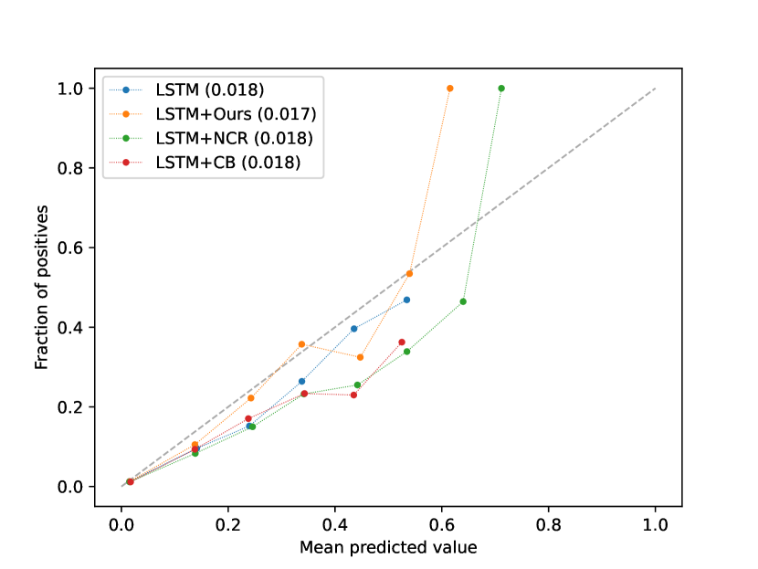
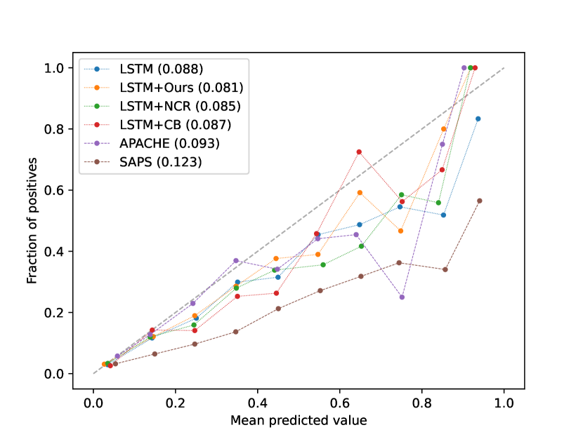
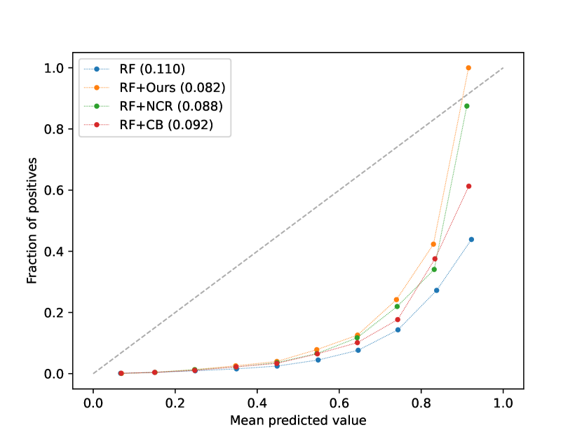
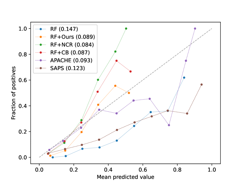
Calibration

Calibration of machine learning models compares the distribution of the probability predicted by models with the distribution of probabilities observed in real data (e.g. real patients). To measure model calibration, we use the Brier score[26] (the lower the better). Our investigation of the respective calibration curves (see Figure 2 and Figure A2) shows that phenotypes from unstructured notes improve model calibration across setups, especially for physiological decompensation and in-hospital mortality, which means the distribution predicted by models is closer to real distribution of patients. Besides, LSTM overall also produces better calibration than RF.

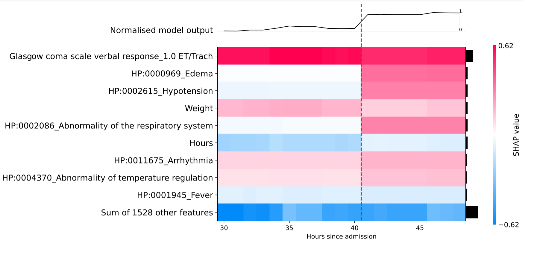
Prognosis analysis

Beyond producing clinically relevant explanations at the cohort level, with the help of SHAP values we can shed light onto a patient’s journey and discover retrospectively when the patient was the most vulnerable and why. For example, the fragment of a patient’s LOS forecast in Figure 3 illustrates an estimated probability, after 41 hour from admission, of a LOS longer than 14 days being of 69%, mainly because the patient scored 1 in the Glasgow Coma Scale Verbal Response. One hour after, when a clinical note becomes available, worrisome phenotypes appear (including edema, hypotension and abnormality of the respiratory system). Consequently, the estimated probability increases to 88%.

Cohort study

We assess performance of our approach to the cohorts of the patients with different diseases especially underrepresented diseases to understand its robustness and generalisability. The test set is split into four disease-specific cohorts for patients with cardiovascular diseases, diabetes, cancer, and depression, and then the accuracies of the best LSTM models (using structured features and phenotypic features) are reported individually for each cohort on each ICU task. We notice the patient number of cardiovascular diseases or diabetes is at least twice that of cancer and around five times that of depression.

For in-hospital mortality and physiological decompensation, we observe comparable accuracies across the four cohorts. We report the range of AUC-ROC between 0.780 and 0.826 for in-hospital mortality and between 0.792 and 0.820 for physiological decompensation for the four cohorts. In contrast, for LOS, we observe lower Kappa 0.321 and 0.330 for small cohorts cancer and depression, respectively, as opposed to 0.413 and 0.424 for larger cohorts with cardiovascular diseases and diabetes. We hypothesise the nature of diseases has strong implication on in-hospital mortality and physiological decompensation while LOS can be influenced by more factors which require larger data samples to model their interactions. The full results are available in Table A7.

Limitations

We have investigated only one data source, MIMIC-III, and our observations are to be confirmed with other data sources.

The analysis on phenotype importance is produced on the Random Forest, whose accuracy is superior than the baselines but not as good as LSTM. This is limited by the poor computation efficiency of SHAP values for LSTM and the explanations from neural network based models are to be investigated in future studies.

Moreover, the phenotypes annotated as transient are made present only until a new clinical note appears in the timeline. This has the inconvenience that phenotypes might be prematurely considered as not present because the next available clinical note did not mention them. Even though the LSTM classifier is able to learn temporal correlations on its own, a more elaborated feature modelling could prove useful.

Acknowledgements

We would like to thank Dr. Rick Sax, Dr. Garima Gupta and Dr. Matt Wiener for their feedback throughout this research. We would also like to thank Dr. Garima Gupta, Dr. Deepa (M.R.S.H) and Dr. Ashok (M.S.) for helping us create gold-standard phenotype annotation data.

Author contributions

JZ, LB, AT and JI conceived the experiments. LB and AT conducted the experiments. JZ, LB, AT, and JI analysed the results. JI, VB and YG reviewed the research and manuscript. All authors approved the manuscript.

Additional information

Competing interests: This study is under collaboration with Imperial College London, Queen Mary University of London, Hong Kong Baptist University and Pangaea Data Limited.

References

[1] Nhs digital annual report and accounts 2019 to 2020 (2020).
[2] Johnson, A. E. et al. Machine learning and decision support in critical care. \JournalTitleProceedings of the IEEE 104, 444–466, DOI: 10.1109/JPROC.2015.2501978 (2016).
[3] Kong, H. J. Managing unstructured big data in healthcare system. \JournalTitleHealthcare Informatics Research 25, 1–2, DOI: 10.4258/hir.2019.25.1.1 (2019).
[4] Harutyunyan, H., Khachatrian, H., Kale, D. C., Ver Steeg, G. & Galstyan, A. Multitask learning and benchmarking with clinical time series data. \JournalTitleScientific data 6, 1–18 (2019).
[5] Subudhi, S. et al. Comparing machine learning algorithms for predicting icu admission and mortality in covid-19. \JournalTitlenpj Digital Medicine 4, 87, DOI: 10.1038/s41746-021-00456-x (2021).
[6] Alves, T., Laender, A., Veloso, A. & Ziviani, N. Dynamic prediction of icu mortality risk using domain adaptation. In 2018 IEEE International Conference on Big Data (Big Data), 1328–1336, DOI: 10.1109/BigData.2018.8621927 (2018).
[7] Robinson, P. N. Deep phenotyping for precision medicine. \JournalTitleHuman mutation 33, 777–780 (2012).
[8] Cooley-Rieders, K. & Zheng, K. Physician documentation matters. using natural language processing to predict mortality in sepsis. \JournalTitleIntelligence-Based Medicine 5, 100028, DOI: 10.1016/j.ibmed.2021.100028 (2021).
[9] Liu, C. et al. Ensembles of natural language processing systems for portable phenotyping solutions. \JournalTitleJournal of Biomedical Informatics 100, 103318, DOI: https://doi.org/10.1016/j.jbi.2019.103318 (2019).
[10] Alsentzer, E. et al. Publicly Available Clinical {BERT} Embeddings. In Proceedings of the 2nd Clinical Natural Language Processing Workshop, 72–78, DOI: 10.18653/v1/W19-1909 (Association for Computational Linguistics, Minneapolis, Minnesota, USA, 2019).
[11] Köhler, S. et al. The human phenotype ontology in 2021. \JournalTitleNucleic Acids Research 49, D1207–D1217, DOI: 10.1093/nar/gkaa1043 (2021).
[12] Lundberg, S. M. & Lee, S.-I. A unified approach to interpreting model predictions. In Guyon, I. et al. (eds.) Advances in Neural Information Processing Systems, vol. 30 (Curran Associates, Inc., 2017).
[13] Johnson, A. E. et al. Mimic-iii, a freely accessible critical care database. \JournalTitleScientific Data 3, 1–9, DOI: 10.1038/sdata.2016.35 (2016).
[14] Zhang, J. et al. Self-supervised detection of contextual synonyms in a multi-class setting: Phenotype annotation use case. In Proceedings of the 2021 Conference on Empirical Methods in Natural Language Processing, 8754–8769 (Association for Computational Linguistics, Online and Punta Cana, Dominican Republic, 2021).
[15] Arbabi, A., Adams, D. R., Fidler, S. & Brudno, M. Identifying clinical terms in medical text using ontology-guided machine learning. \JournalTitleJMIR medical informatics 7, e12596 (2019).
[16] Breiman, L. Random forests. \JournalTitleMachine Learning 45, 5–32, DOI: 10.1023/A:1010933404324 (2001).
[17] Hochreiter, S. & Schmidhuber, J. Long short-term memory. \JournalTitleNeural Computation 9, 1735–1780, DOI: 10.1162/neco.1997.9.8.1735 (1997).
[18] Lasko, T. A., Bhagwat, J. G., Zou, K. H. & Ohno-Machado, L. The use of receiver operating characteristic curves in biomedical informatics. \JournalTitleJournal of Biomedical Informatics 38, 404–415, DOI: 10.1016/j.jbi.2005.02.008 (2005).
[19] Cohen, J. A coefficient of agreement for nominal scales. \JournalTitleEducational and Psychological Measurement 20, 37–46, DOI: 10.1177/001316446002000104 (1960).
[20] Pham-Gia, T. & Hung, T. L. The mean and median absolute deviations. \JournalTitleMathematical and Computer Modelling 34, 921–936, DOI: 10.1016/S0895-7177(01)00109-1 (2001).
[21] Kramer, A. A. Are icu length of stay predictions worthwhile? \JournalTitleCritical Care Medicine 45, 379–380, DOI: 10.1097/CCM.0000000000002111 (2017).
[22] Forte, J. C. & van der Horst, I. C. Comorbidities and medical history essential for mortality prediction in critically ill patients. \JournalTitleThe Lancet Digital Health 1, e48–e49, DOI: 10.1016/S2589-7500(19)30030-5 (2019).
[23] Nielsen, A. B. et al. Survival prediction in intensive-care units based on aggregation of long-term disease history and acute physiology: a retrospective study of the danish national patient registry and electronic patient records. \JournalTitleThe Lancet Digital Health 1, e78–e89, DOI: 10.1016/S2589-7500(19)30024-X (2019).
[24] Georgiou, E., Hadjibalassi, M., Lambrinou, E., Andreou, P. & Papathanassoglou, E. D. The impact of pain assessment on critically ill patients’ outcomes: A systematic review. \JournalTitleBioMed Research International 2015, DOI: 10.1155/2015/503830 (2015).
[25] Bastos, P. G., Sun, X., Wagner, D. P., Wu, A. W. & Knaus, W. A. Glasgow coma scale score in the evaluation of outcome in the intensive care unit: Findings from the acute physiology and chronic health evaluation iii study. \JournalTitleCritical Care Medicine 21, 1459–1465, DOI: 10.1097/00003246-199310000-00012 (1993).
[26] BRIER, G. W. Verification of forecasts expressed in terms of probability. \JournalTitleMonthly Weather Review 78, 1 – 3, DOI: 10.1175/1520-0493(1950)078<0001:VOFEIT>2.0.CO;2 (1950).
[27] Lundberg, S. M. et al. From local explanations to global understanding with explainable ai for trees. \JournalTitleNature Machine Intelligence 2, 56–67, DOI: 10.1038/s42256-019-0138-9 (2020).

Appendix

Shapley Values

Shapley values come from game theory and are used to estimate the impact of a feature on a system’s output. Feature impact is defined as the variation in the output of the model when the feature is observed versus when it is unknown.

Shapley values belong to a category of methods denominated additive. In particular, the additivity is formulated as

\begin{split}f(x)&=\phi_{0}(f,x)+\sum_{i=1}^{M}\phi_{i}(f,x)\end{split}

where $f(x)$ is the prediction made by the model, $x$ are the features fed to the model, $M$ is the number of features, $\phi_{i}$ is the Shapley value of the i-th feature, and $\phi_{0}=E[f(x)]$ is the expected value of the model over the training dataset. Also, this assumption ensures the values correctly reflect the difference between the expected model output and the output for a particular prediction.

The Shapley value of a feature is computed via

\begin{split}\phi_{i}(f,x)&=\sum_{S\subseteq S_{all}/\{i\}}\frac{|S|!(M-|S|-1)!}{M!}[f_{x}(S\cup\{i\})-f_{x}(S)]\\ &=\sum_{S\subseteq S_{all}/\{i\}}\frac{1}{(M\text{ choose }|S|)(M-|S|)}[f_{x}(S\cup\{i\})-f_{x}(S)]\end{split}

(1)

where $S$ is a subset of all $M$ input features, and $f_{x}(S)=E[f(x)|x_{s}]$ with $x_{s}$ in a subset of the input features with only those belonging to $S$ present.

In this study we used the SHAP library [12] and its optimisation for tree-based classifiers [27] to compute the Shapley values.

.2 Data distribution by splits

	Counts
Task	Split	Patients	ICU Episodes	Timesteps	Labels
Task	Split	Patients	ICU Episodes	Timesteps	Positive	Negative
Physiological Decompensation	CV-1	5125	6215	528425	10283	518142
	CV-2	5129	6134	507892	10821	497071
	CV-3	5141	6264	511289	10426	500863
	CV-4	5102	6297	527853	11020	516833
	Test	3683	4463	367533	6931	360602
In-Hospital Mortality	CV-1	2929	3382	162063	441	2941
	CV-2	2917	3331	159566	466	2865
	CV-3	2888	3356	160732	439	2917
	CV-4	2936	3410	163284	477	2933
	Test	2119	2453	117500	283	2170
Length of Stay	CV-1	5151	6245	532403	Refer to Table A2
	CV-2	5145	6154	510227
	CV-3	5160	6286	514147
	CV-4	5117	6314	530331
	Test	3698	4483	369350

Table A1: Data distribution by splits. For the physiological decompensation and length of stay tasks, timesteps are taken as samples as the predictions are made every hourly timesteps, while for the in-hospital mortality task, ICU episodes are taken as samples as the predictions are made at a fixed timestep. Here, CV refers to the training Cross-Validation Folds.

.3 Class distribution for length of stay

Class Label	Class Description (Days)	CV-1	CV-2	CV-3	CV-4	Test
0	<1	131913	129634	131693	133186	95439
1	1 - 2	85311	83558	84065	85818	61372
2	2 - 3	56353	54074	54007	54780	38858
3	3 - 4	39416	37605	38106	38054	27142
4	4 - 5	29384	27982	28760	28573	20171
5	5 - 6	22830	22384	22360	22626	15878
6	6 - 7	18816	18612	18626	18582	12940
7	7 - 8	15925	15583	15697	15863	10953
8	8 - 14	62655	58512	59905	60611	40856
9	>14	69800	62283	60928	72238	45741
Total		532403	510227	514147	530331	369350

Table A2: Class distribution for Length of Stay

Algorithm hyperparameters

Classifier	Hyperparameters
Random Forest	num of estimators=300, criterion="gini", max depth=None, min samples split=2, min samples leaf=1
LSTM	epochs=30, hidden size=128, batch size=8, num of layers=1, patience=10, dropout rate=0, learning rate=1e-4, weight decay=0.0

Table A3: Hyperparameters for classifiers

Significance tests

ML Classification Model

Base Model

Secondary Models

S +

NCR

S +

Ours

Random Forest

13.25

S + NCR

94.82

26.13

S + CB

86.75

5.18

1.07

S + Ours

100

73.87

98.93

LSTM

S + NCR

100

S + CB

100

S + Ours

100

(a) In-Hospital Mortality

ML Classification Model

Base Model

Secondary Models

S +

NCR

S +

Ours

Random Forest

81.4

S + NCR

18.6

32.4

S + CB

67.6

S + Ours

100

LSTM

S + NCR

100

S + CB

100

S + Ours

100

(b) Physiological Decompensation

ML Classification Model

Base Model

Secondary Models

S +

NCR

S +

Ours

Random Forest

22.1

100

S + NCR

77.9

100

S + CB

S + Ours

100

LSTM

S + NCR

100

S + CB

100

S + Ours

100

Table A4: Statistical Significance Matrix with Bootstrap Resampling. All the scores are percentages of samples where the base model performs better than the secondary model. Each sample is built by resampling the original test set and then scoring the base/secondary model on it. For example, the last row in (a) shows the base model (LSTM with S + Ours) is better than the secondary models (LSTM with S or S + NCR or S + CB) on 100% samples (i.e. with statistical significance). Here, S refers to Structured, NCR to Neural Concept Recognizer[15], CB to ClinicalBERT, and Ours to our phenotyping model.

4-Fold cross validation results

Classification Model	Features Design	4-Fold Cross Validation Aggregate
	Features Design	AUC-ROC		AUC-PR
		Mean	SD	Mean	SD
SAPS-II	-	0.754	0.006	0.322	0.031
APACHE-III	-	0.732	0.008	0.326	0.018
Random Forest	S	0.810	0.008	0.418	0.018
	S + NCR	0.819	0.014	0.472	0.013
	S + CB	0.804	0.012	0.423	0.005
	S + Ours	0.834	0.008	0.477	0.016
LSTM	S	-	-	-	-
	S	0.829	0.007	0.441	0.016
	S + NCR	0.836	0.011	0.478	0.008
	S + CB	0.829	0.007	0.459	0.007
	S + Ours	0.845	0.004	0.496	0.014

(a) In-hospital mortality

Classification Model	Features Design	4-Fold Cross Validation Aggregate
		AUC-ROC		AUC-PR
		Mean	SD	Mean	SD
Random Forest	S	0.815	0.003	0.127	0.009
	S + NCR	0.820	0.003	0.125	0.007
	S + CB	0.818	0.004	0.123	0.008
	S + Ours	0.844	0.004	0.165	0.013
LSTM	S	-	-	-	-
	S	0.819	0.003	0.136	0.016
	S + NCR	0.820	0.003	0.134	0.013
	S + CB	0.821	0.006	0.128	0.022
	S + Ours	0.833	0.008	0.144	0.023

(b) Physiological decompensation

Classification Model	Features Design	4-Fold Cross Validation Aggregate
		Kappa		MAD
		Mean	SD	Mean	SD
Random Forest	S	0.381	0.005	142.010	4.665
	S + NCR	0.382	0.008	148.003	4.180
	S + CB	0.369	0.005	149.221	3.789
	S + Ours	0.405	0.006	116.940	5.674
LSTM	S	-	-	-	-
	S	0.375	0.003	134.373	17.293
	S + NCR	0.393	0.013	127.165	17.484
	S + CB	0.374	0.015	127.678	8.608
	S + Ours	0.416	0.012	116.198	6.904

Table A5: Results for (a) In-Hospital Mortality, (b) Physiological Decompensation, and (c) Length of Stay on the training set. The best score for each classifier is highlighted in bold. Here, S refers to Structured, NCR to Neural Concept Recognizer[15], CB to ClinicalBERT, and Ours to our phenotyping model.

.4 Ablation study on phenotype persistency

Model	Phenotypic propagation	4-fold Cross Validation Aggregate				Test Set
		AUC-ROC		AUC-PR		AUC-ROC	AUC-PR
		Mean	SD	Mean	SD	AUC-ROC	AUC-PR
RF	without	0.807	0.008	0.413	0.021	0.799 (0.772, 0.824)	0.351 (0.297, 0.407)
RF	with	0.834	0.008	0.477	0.016	0.845 (0.826, 0.873)	0.462 (0.404, 0.524)
LSTM	without	0.833	0.014	0.457	0.024	0.831 (0.807, 0.853)	0.421 (0.361, 0.483)
LSTM	with	0.844	0.004	0.495	0.013	0.845 (0.823, 0.868)	0.464 (0.405, 0.523)

(a) In-hospital Mortality

Model	Phenotypic propagation	4-fold Cross Validation Aggregate				Test Set
		AUC-ROC		AUC-PR		AUC-ROC	AUC-PR
		Mean	SD	Mean	SD	AUC-ROC	AUC-PR
RF	without	0.812	0.002	0.125	0.007	0.820 (0.815, 0.825)	0.127 (0.120, 0.135)
RF	with	0.844	0.004	0.165	0.013	0.845 (0.840, 0.850)	0.180 (0.171, 0.190)
LSTM	without	0.827	0.007	0.146	0.017	0.841 (0.842, 0.851)	0.149 (0.141, 0.156)
LSTM	with	0.833	0.007	0.144	0.022	0.839 (0.834, 0.844)	0.145 (0.138, 0.153)

(b) Physiological Decompensation

Model	Phenotypic propagation	4-fold Cross Validation Aggregate				Test Set
		Kappa		MAD		Kappa	MAD
		Mean	SD	Mean	SD	Kappa	MAD
RF	without	0.376	0.005	139.8	5.5	0.386 (0.380, 0.384)	135.0 (134.5, 135.6)
RF	with	0.405	0.006	116.9	5.6	0.420 (0.418, 0.422)	110.3 (109.3, 111.3)
LSTM	without	0.427	0.007	118.3	4.2	0.441 (0.439, 0.440)	111.4 (110.9, 111.9)
LSTM	with	0.416	0.012	116.2	6.9	0.430 (0.427, 0.432)	116.7 (116.2, 117.3)

Table A6: Results of ablation study on our phenotyping model to assess the importance of phenotypic modelling. Models without phenotypic propagation encounter high sparsity of phenotypes as data is only available at the timestep the clinical note is written. Models with phenotypic propagation observe phenotypes throughout all timesteps. The best score for each classifier is highlighted in bold.

Feature importance for Length-of-Stay

Calibration curves

.5 Cohort study

Cohort	No. of Patients	No. of ICU Episodes	AUC-ROC
All	2119	2453	0.845
Cardiovascular Diseases	681	789	0.780
Diabetes	563	682	0.826
Cancer	277	304	0.822
Depression	119	122	0.783

(a) In-hospital Mortality.

Cohort	No. of Patients	No. of ICU Episodes	AUC-ROC
All	3683	4463	0.839
Cardiovascular Diseases	975	1197	0.792
Diabetes	927	1191	0.808
Cancer	489	565	0.806
Depression	216	240	0.820

(b) Physiological Decompensation.

Cohort	No. of Patients	No. of ICU Episodes	Kappa
All	3698	4483	0.430
Cardiovascular Diseases	980	1202	0.413
Diabetes	930	1195	0.424
Cancer	493	572	0.321
Depression	216	241	0.330

Table A7: Analysing the generalisability and robustness of our approach on cohorts with different diseases. The accuracies of the best LSTM models which use features from both structured and unstructured data are reported individually on each cohort for each ICU task.

Clinical Utility of the Automatic Phenotype Annotation in Unstructured Clinical Notes: ICU Use Cases

Abstract

Objective

Methods

Results

Conclusion

Summary

Introduction

Methodology

0.1 Data preprocessing

Algorithm development and analysis

Evaluation Metrics

Model evaluation and statistical analysis

Results

Phenotyping

Quantitative results

Discussion

Phenotype persistency

Phenotype importance

Calibration

Prognosis analysis

Cohort study

Limitations

Acknowledgements

Author contributions

Additional information

References

Appendix

Shapley Values

.2 Data distribution by splits

.3 Class distribution for length of stay

Algorithm hyperparameters

Significance tests

4-Fold cross validation results

.4 Ablation study on phenotype persistency

Feature importance for Length-of-Stay

Calibration curves

.5 Cohort study

.6 Forecasts per total length of stay

.7 Case study for physiological decompensation