Balmer continuum enhancement detected in a mini flare observed with IRIS

Abstract

Context. Optical and near-UV continuum emissions in flares contribute substantially to flare energy budget. Two mechanisms play an important role for continuum emission in flares: hydrogen recombination after sudden ionization at chromospheric layers and transportation of the energy radiatively from the chromosphere to lower layers in the atmosphere, the so called back-warming.

Aims. The aim of the paper is to disentangle between these two mechanisms for the excess of Balmer continuum observed in a flare.

Methods. We combine the observations of Balmer continuum obtained with the Interface Region Imaging Spectrograph (IRIS) (spectra and slit-jaw images (SJIs) 2832 Å) and hard X-ray (HXR) emission detected by FERMI Gamma Burst Monitor (GBM) during a mini flare. Calibrated Balmer continuum is compared to non-LTE radiative transfer flare models and radiated energy is estimated. Assuming thick target HXR emission, we calculate the energy of non-thermal electrons detected by FERMI GBM and compare it to the radiated energy.

Results. The favorable argument of a relationship between the Balmer continuum excess and the HXR emission is that there is a good time coincidence between both of them. In addition, the shape of the maximum brightness in the 2832 SJIs, which is mainly due to this Balmer continuum excess, is similar to the FERMI/GBM light curve. The electron-beam flux estimated from FERMI/GBM between 10⁹ to 10¹⁰ erg s^-1 cm^-2 is consistent with the beam flux required in non-LTE radiative transfer models to get the excess of Balmer continuum emission observed in this IRIS spectra.

Conclusions. The low energy input by non thermal electrons above 20 keV is sufficient to produce the enhancement of Balmer continuum emission. This could be explained by the topology of the reconnection site. The reconnection starts in a tiny bald patch region which is transformed dynamically in a X-point current sheet. The size of the interacting region would be under the spatial resolution of the instrument.

1 Introduction

Heating of the lower solar atmosphere during solar flares is an interesting and still open area in solar Physics, as it deals with the energy distribution in flares. That is directly related to the radiation emitted during a solar flare. The heated atmosphere produces the enhancement of emission in many lines and continua. The origin of optical continuum in flares comes from two mechanisms: the hydrogen recombination as for continua (Paschen, Balmer) in the chromosphere and H^- emission in the photosphere. The optical continuum enhancement is a reliable signature of the so-called white light flare (WLF, Fletcher et al., 2011). Enhancement of the Balmer continuum below 3646 Å has been reported in ground based observations of flares (Neidig, 1989) and recently in the Interface Region Imaging Spectrograph (IRIS, De Pontieu et al., 2014) spectra during strong X-class WLF (Heinzel & Kleint, 2014; Kleint et al., 2016, 2017). Electron beams are often invoked to explain the WLF heating in the low chromosphere and photosphere. The enhancement of the Balmer continuum emission is produced in higher levels in the chromosphere. In Heinzel & Kleint (2014) there is a comparison of the enhancement of the Balmer continuum with the light curves from RHESSI and a good spatial and temporal correlation is found, which is explained by electron-beam heating and ionizing the chromosphere. Then the subsequent recombination leads to Balmer-continuum emission. It is the chromosphere which could produce the Balmer continuum emission enhancement, while the photosphere may in some cases produce the white-light emission which is probably due to radiative backwarming (Machado et al., 1989). This issue was discussed earlier in Ding et al. (2003); Heinzel & Kleint (2014) and quantitatively modelled in Kleint et al. (2016).

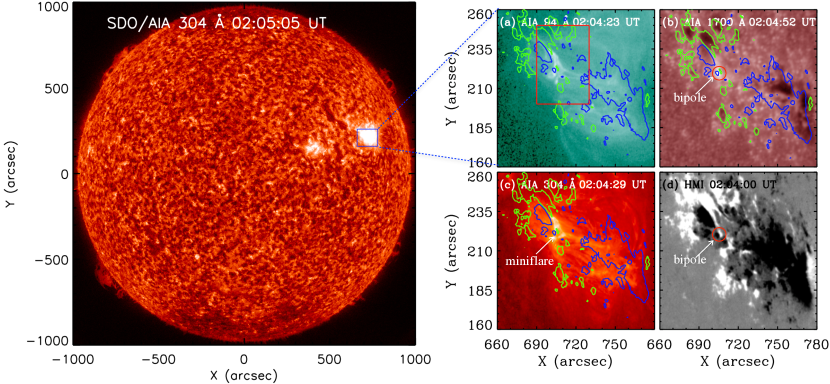
Figure 1: Active region AR NOAA 12736 observed with AIA on March 22, 2019. (Left panel): full disk in 304 Å, the blue box (field of view of the right panels) contains the only AR visible on the disk on that day. (Right panels a, b, c): images of the AR in different AIA filters, respectively in 94 Å, 1700 Å  and 304 Å  superimposed with the contours of the magnetic field of strength $\pm$ 300 Gauss. Panel (d): magnetic field observed with HMI. The bipole (small circle in panels (b) and (d)) is responsible of the reconnection. The mini flare is indicated by an arrow in panel (c). The box in panel (a) is the field of view of Fig. 2.

A quasi-continuous enhancement in flares can be interpreted in three different ways. (i) it may be the Balmer continuum emission, superposed over the background spectrum. (ii) the continuum is due to contribution from the photosphere either by direct beam bombardement (but this could take place only for strong beams, such as in strong flares) or by radiative backwarming. (iii) finally the enhancement could be influenced by the emission of broad wings of Mg II lines. Heinzel & Kleint (2014) took the advantage to use the IRIS 2832 Å  band spectra where the Mg II wings were not present to identify the real Balmer continuum excess at an X-class flare site.

Recently a micro flare observed in multiple wavelengths by SDO/AIA and IRIS puzzled us as the Balmer continuum seems also to be enhanced, even in a weak flare. This micro flare that we called mini flare in the previous papers occurred at the base of a solar jet on March 22, 2019. The analysis of the vector magnetic field revealed the existence of a flux rope in the vicinity of the jet and the magnetic reconnection took place in a bald patch region where magnetic field lines were tangential to the photosphere (Joshi et al., 2020).

The proper motions of the photospheric magnetic polarities suggested that the twist of the flux rope was transferred during reconnection to the jet generating a twisted jet. A detail spectroscopic analysis of the mini flare associated to this jet was carried out with IRIS spectra (Joshi et al., 2021), Using the cloud model technique applied to the Mg II line profiles we identified explosive clouds with supersonic Alfvén velocities. A stratification thermal model of the atmosphere at the time of the reconnection was proposed. The Mg II spectra show extended wings like in IRIS bombs (Peter et al., 2014; Grubecka et al., 2016). Twist and bald patch reconnection was confirmed with the analysis of the IRIS spectra (Si IV, C II, Mg II) by Joshi et al. (2020).

In this paper we extend the IRIS data analysis of the mini flare studied in Joshi et al. (2020, 2021) and present the Balmer continuum around 2832 Å observed with IRIS (Sect. 2). Section 3 presents the IRIS spectra and 2832 Å slit-jaw images (SJIs) analysis. Further, we analysed the hard X-ray (HXR) emission detected by FERMI/GBM (Sect. 4). We discuss on the possible non-LTE radiative transfer models, proposed in Kleint et al. (2016), deriving the radiated energy from the measurements of the Balmer continuum. We compare the radiative energy to the energy contained in non-thermal electrons as derived from HXR measurements. In conclusion we conjecture that the Balmer continuum enhancement is due to the energy electron deposit produced during the flare (Sect. 5). We suggest that the energy deposit, even with a relatively low value is sufficient because the reconnection is located in the low layers of the atmosphere in a tiny bald patch region as the magnetic topology of the region revealed (Joshi et al., 2020).

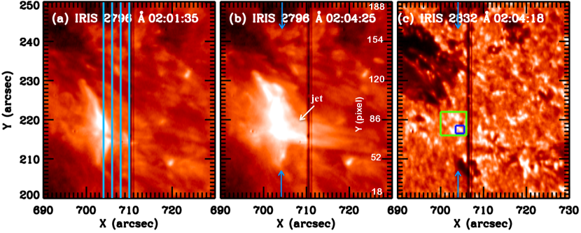
Figure 2: IRIS SJI of the mini flare in 2796 Å  (panels a-b) and 2832 Å  (panel c) filters respectively. In panel (a) the four vertical cyan lines are the four IRIS slit positions of the rasters. The vertical cyan arrows in panel (b-c) indicate the IRIS slit position 1, which crosses the mini flare (bipole) region presented in Fig. 1 (panels b- d). The green and blue boxes in panels (c) are the fields of view used to compute the light curves of the bright point in Fig. 4.

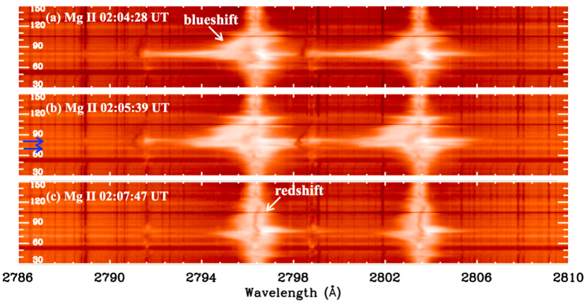
Figure 3: Spectra of Mg II lines h and k in the Balmer continuum full wavelength range of IRIS (50 Å) during and after the mini flare times at the reconnection site along the first slit position (Fig. 2 panels a-c)). Bidirectional outflows are observed at the reconnection point (y=80 in panel a). Balmer continuum emission is visible in the three panels at two different pixels (y= 70, 80) in wavelengths 10 Å far from the k line core (see in panel b the two horizontal blue arrows). Blueshifts, and redshifts indicated by two white arrows in the Mg II k line wings correspond to the twisted expelled jet and material falling back (panels a and c).

2 Co-temporal observations

2.1 AIA and IRIS SJI

The mini flare (GOES B6.7) occurred in the active region (AR NOAA 12736), which was located at N09 W60 on March 22, 2019. It was the only AR in the whole solar disk on that day (Figure 1 left panel). The Atmospheric Imaging Assembly (AIA, Lemen et al., 2012) on board the Solar Dynamics Observatory (SDO, Pesnell et al., 2012) allows us to display the images of the mini flare in all the channels from UV (1600 and 1700 Å) to EUV (94 Å, 131 Å, 171 Å, 193 Å, 211 Å, and 304 Å) covering a broad temperature range from 4500 K to 10⁶ K (Fig. 1 a-c). The 1700 Å filter contains hotter coronal lines which are in emission in strong flares leading to enhancement of flare brightenings in this filter (Simões et al., 2019). Our mini flare being a weak flare we may guess for a high probability that the enhancement visible at 1700 Å is due to heating of the plasma in the minimum temperature region around 4500 K. The topological configuration of the AR was analysed previously (Joshi et al., 2020) showing that the AR formed by successive emerging magnetic fluxes (EMFs) adjacent to each other. The inversion line between two opposite polarities belonging to two different EMFs was the site of strong shear and magnetic reconnection, a small bipole was identified as the origin of the mini flare in HMI magnetograms (Fig. 1 d). The mini flare is in the central part of a bright, more or less north-south semi circle overlying the inversion line between positive and negative polarities.
IRIS contains three CCDs for the far ultra-violet (FUV) and near ultra-violet (NUV) spectra and one CCD for the SJIs. IRIS performed medium coarse rasters of 4 steps from 01:43:27 UT to 02:42:30 UT centered at x=709$\arcsec$ and y=228$\arcsec$ in the SJI field of view of 60$\arcsec$ $\times$ 68$\arcsec$. The raster step size is 2^′′ so each spectral raster spans a field of view of 6 ^′${}^{\prime}\times$ 62 ^′′. The nominal spatial resolution is 0.^′′33. IRIS SJIs in Mg II 2896 filter and in 2832 Å continuum filter are recorded with a 14 sec cadence (see examples in Fig. 2 a-c). The four slits are drawn in panel a. The first slit on the left crosses the mini flare. Slits 2, 3, 4 cross the jet on the right. In 2832 continuum filter small bright dots are observed at the location of the mini flare (green and blue boxes). For an accurate comparison between the AIA images and IRIS SJIs we manually align these images by shifting the IRIS SJIs by 4$\arcsec$ in x-axis and 3$\arcsec$ in y-axis, as noted in the previous paper (Joshi et al., 2021). The relationship between heliographic coordinates and pixels along the slit of the spectra is shown in Figure 2 (b).

The IRIS Mg II spectra during the mini flare were analysed in Joshi et al. (2021). Bidirectional flows ($\pm$ 200 km s^-1) were observed at the flare reconnection site covering one or two pixels y= 79-80 at 02:03:46 UT. At 02:04:28 UT strong blueshifts in pixels $>80$ and redshifts a few minutes later were also observed, which we interpret as material of the jet going up and then falling back. The mini flare is definitively not a double-ribbon flare with many ribbons as it is the case in Kleint et al. (2017). A bright continuum is detected all along the wavelength domain in the Mg II spectra at the flare site (y = 70 and 80 pixel) during a few minutes (Fig. 3). In this study we focus on the Balmer continuum far away from the extended Mg II line wings until 2835 Å to be free of the emission of the Mg II line wings.

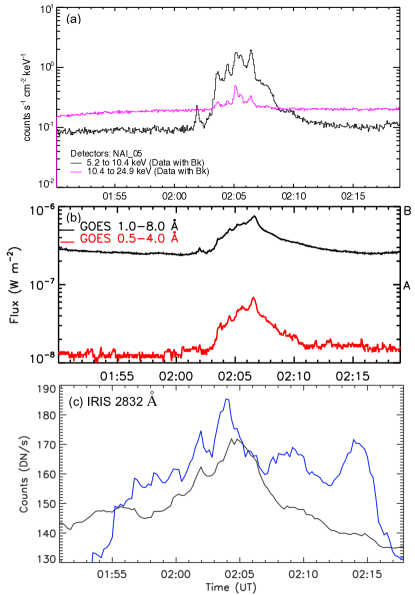
Figure 4: Intensity variation at the flare site observed in FERMI GBM, GOES, and IRIS SJIs. Panel(a): X-ray count rates detected in two energy channels by FERMI/GBM.. Panel (b): GOES light curve for the B6.7 class solar flare, shows the flare starts at 02:02 UT and peaks at $\approx$ 02:06 UT with small peaks corresponding to GBM peaks. Panel (c): Intensity light curves at the bright points in the IRIS 2832 Å  SJIs. The black and blue curves are the light curves over the green and blue boxes presented in Fig. 2 (d) respectively. The DN signal at the flare base is integrated and divided by the total number of pixels.

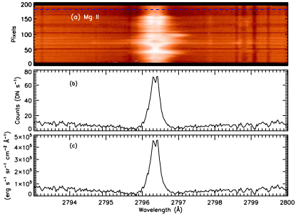
Figure 5: Mg II k line spectra along the slit at 01:43:41 UT before the flare (a). Panels (b) and (c) show the Mg II k line profiles in position y = 180 pixel representing the quiet sun in DN s^-1 and in cgs units, respectively.

2.2 Mini flare light curves

We first check the occurrence times of the soft X-ray (SXR) and HXR peaks with the bright point intensity observed in the 2832 Å filter by comparing the time variation of X-ray flux with the intensity light curve of 2832 Å filter between 01:44 UT and 02:20 UT (Fig. 4). The SXR light curve of the flare is recorded by GOES spacecraft in 0.5–4 Å and 1–8 Å. The HXR count rates in different energy bands are recorded with the Gamma-ray Burst Monitor (GBM, Meegan et al., 2009) on board FERMI spacecraft launched in 2008. FERMI GBM fills the gap for HXR measurements for the solar physics community after the decommissioning of RHESSI. FERMI GBM does not provide HXR images like RHESSI so we cannot check if the HXR emission comes from the flaring active region, but at that time only one active region was present on the solar disk (Fig 1 left panel) so the HXR emission is expected to come from the flaring active region. In the bottom panel of Fig. 4, Mg II 2832 Å slit jaw intensity light curves are obtained by integrating the DN signal divided by the total number of pixels in the small boxes at the flare site (Fig. 2 green and blue boxes). We conclude on a good agreement between the occurrence times of the Balmer continuum enhancement, HXR emission and the GOES light curves for this flare.

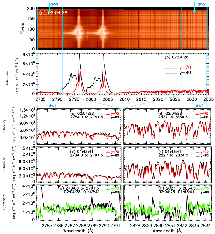
Figure 6: Flare intensity distribution in the IRIS Mg II wavelength band at the flare time (02:04:28 UT). Panel (a) shows the full spectra of the Mg II band between $\lambda$= 2784 Å and $\lambda$ =2835 Å (50 Å) along slit 1 position. Two dashed horizontal black lines indicate the coordinates y= 70 and y = 80 at the location of the maximum of the Balmer continuum in the spectral image. Panel (b) presents the spectral profile in the full range of the IRIS Mg II wavelength band at the two positions (y = 70 and 80 pixels). Panels (c) and (d) show the zoom of two spectral profiles of panel (b) at (y= 70, 80) located at the two extremities of the wavelength band (dw1, dw2) indicated by two vertical cyan lines and two cyan arrows at the top of panel (a), respectively in the right and in the left of the panel. Panel (e) and (f) show the similar zoom spectra in the two continuum regions at the pre flare time (01:43:41). Panel (g) and (h) show the difference of intensity ($\Delta$(Intensity)) between the intensity at the flare time (02:04:28 UT) and at the preflare time (01:43:41 UT). The intensity is calibrated to the c.g.s. units, i.e. erg s^-1 sr^-1 cm^-2 Å^-1.

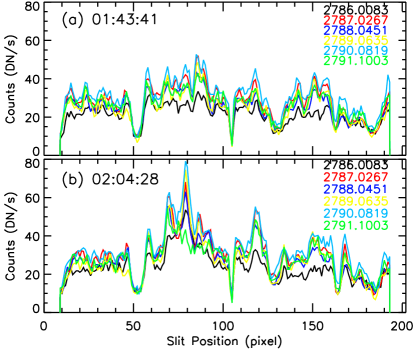
Figure 7: Flare intensity variation along the IRIS slit at different wavelengths at the pre-flare (01:43:41 UT) (panel a) and flare (02:04:28 UT) (panel b) times. The different colors of the curves are for the different wavelengths. The intensity variation shows a constancy during the pre-flare time, whereas the curve shows two peaks at y= 70 and 80 pixel during the flare time. The counts are minimum at the slit position y= 180 pixel. These three positions are chosen as the reference of the quiet sun and the Balmer enhancement respectively.

3 Balmer Continuum enhancement

As it is said in the introduction, the enhancement of the Balmer continuum can be interpreted in different ways. To disentangle between the different mechanisms we need to analyse the IRIS spectra in details (Fig. 3) and calibrate the data for computing quantitatively the excess of the Balmer continuum emission.

3.1 Intensity calibration spectra

Using the IRIS radiometric calibration, we convert the data number (DN) to intensity units. We use the IDL routine iris_calib.pro and get the intensity value (I_c) in erg cm^-2 s^-1 sr^-1 Å^-1. The exposure time per slit position was $\approx$ 2 sec for this conversion. The radiometric intensity calibration is done with a code developed by H. Tian, with the following formula:

$$I_{c}=\frac{hc}{\lambda}\times n\times\frac{I_{o}}{A_{eff}\times d\times\omega}$$ (1)

The photon energy ${hc}/{\lambda}$ is calculated with Planck constant h = 6.63 $\times$ 10^-27 erg-s, speed of light c = 3 $\times$ 10¹⁰ cm s^-1. $n$ is the number of photons per DN, it has a value 4 for FUV and 18 for NUV spectra. I_o is the observed intensity in DN s^-1 and A_eff is the effective area in cm^-2 and obtained through $iris\_get\_response$ routine available in SolarSoftWare (SSW). Dispersion $d$ is taken in Å pixel^-1. The solid angle $\omega$ is calculated as: $\omega=0.3327\times 720\times 0.33\times 720/({1.5\times 10^{8}})^{2}$.

Figure 5 shows the relationship between the DN signal in the range of Mg II k line and the calibrated data for the quiet sun (y = 180 pixel). The Mg II k line peaks at $4.8\times 10^{5}$ erg s^-1 sr^-1 cm^-2 Å^-1. In both ends of the domain the photospheric Mg II wing emission is increasing.

3.2 IRIS spectra before the flare

Figure 8 panel (a) shows the full range of the Mg II window spectra for the quiet sun before the flare at 01:43:41 UT. This spectra will be our reference spectra. The full IRIS wavelength range, focused on the Mg II lines and is extended from 2784 Å to 2835 Å. This large domain allows us to analyse the Balmer continuum relatively far from the cores of the Mg II h and k lines. The spectral profiles of three pixels (y=10, 170, 180) in the quiet sun (Fig. 8 panel b) can be compared to the global sun spectral profile shown in Pereira et al. (2013). Such spectral profile has a U-shape with an increasing emission toward the two extremities of the spectral range, in the blue far wing of k and in the far red wing of h, both emissions corresponding to photosphere emissions (Fig. 8 panels (c) and (d) respectively). In the center of the profile there are the two chromospheric h and k lines cores in emission.

Even for the flare time the spectral profile could be about the same as that detected in the IRIS spectrum outside the flare if there was no Balmer continuum enhancement. The fact that the ”continuum” peaks in time with the HXR emission indicates that there exists a direct relationship between the enhancement of the continuum and the non thermal flux (Fig. 4). However extended wings of Mg II lines during flares may also affect the continuum. Therefore we explore the wavelength range the farthest as possible from k and h line cores during the flare time.

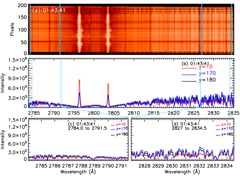
Figure 8: Quiet Sun intensity distribution in the IRIS Mg II wavelength band at the preflare time (01:43:41 UT). Panel (a) shows the full spectra of the Mg II band between $\lambda$= 2784 Å and $\lambda$ =2835 Å (50 Å), the dashed horizontal black lines indicate y= 10, 170, and 180 which represent quiet sun regions. Panel (b) presents the spectral profile of the full range of Mg II lines for the three y pixel values (10, 170, 180). Panels (c) and (d) show the zoom of two parts of the spectral profile at the two ends of the wavelength band, shown by two cyan vertical lines respectively in the right and in the left in panel (a) and (b). The intensity is calibrated in erg s^-1 sr^-1 cm^-2 Å^-1.

3.3 IRIS spectra at the flare time

The site of the flare is crossed by only one slit of the raster (slit 1) as it was shown in Joshi et al. (2021). Figure 6 panel (a) shows the full wavelength range of the Mg II spectra along this slit at the time of the mini flare (02:04:28 UT). The reconnection site is detected by bidirectional outflows, principally blueshifts which concerns one or two pixels along the slit. We note the U-shape profile with an increasing intensity at the two extremities of the wavelength range (Fig. 6 panel (b)), similar behaviour of the spectral profile of the quiet sun (Fig. 8 panel (b)). It is difficult to detect the excess of the continuum emission without proceeding to a subtraction of the quiet sun profile. First we select the pixels where the Balmer continuum enhancement is the more visible. For that we made cuts in the Mg II spectra (Fig.6 panel (a)) for different wavelengths in the continuum in the extreme left and right perpendicularly to the dispersion direction (Fig. 7). Peaks in the continuum at the flare time are well visible for pixels 70 and 80 along the slit, which we select for the following analysis.

By subtracting the background spectra in the whole IRIS Mg II wavelength band observed before the flare (01:43:41 UT) from the spectra during the flare (02:04:28 UT) we get the Balmer-continuum excess. We check that the signal is constant at the boundaries of the domain after the subtraction. Thus two different domains of the continuum are chosen, e.g. 2784-2791.5 Å and 2827-2834.5 Å  to compute the intensity variation (Fig. 6 panels c-d for flare time, in panels e-f for pre-flare time) and finally the subtraction of both intensities (Fig. 6 panels g-h). The difference intensity plots show a constant continuum enhancement in each selected domain of the order of 1.5 to 1.75 $\times$ 10⁵ erg s^-1 sr^-1 cm^-2 Å^-1. The superimposed residual signal is weak, due to optically-thin Balmer emission but significant. The enhancement of the Balmer continuum corresponds to an increase of about 50 $\%$ over the pre-flare level during the flare.

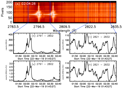
Figure 9: Evolution versus time of the intensity in the Mg II k and in the 2832 Å ranges. Top panel: IRIS spectra of the Mg II band along the slit position 1. The two wavelength regions in Mg II k line (left) and in the Balmer emission (right) are bounded by vertical blue lines. Bottom panels (b-e): temporal evolution of the relative contribution of Mg II k line (b, d) and Balmer continuum emission (c, e) at the reconnection point of the flare (y=80). In panels c and d the intensity (DN) has been divided by the transmission factor f($\lambda$) of the 2832 filter taken from Kleint et al. (2017). The comparison of the relative peak values at the flare time in Mg II range (panel c) and continuum region (panel d) indicates the prevalence of the Balmer continuum.

3.4 IRIS SJI 2832 Å filter

The SJIs in the 2832 Å  filter show a brightening at the location of the flare around 02:05 UT (Fig. 2). In Fig. 4 we estimate the increase of the brightening in the small box (Fig. 2 panel(c)) by 50 $\%$ ((180-120)/120) between the time of the pre-flare (01:44 UT) and the flare time (02:04 UT). The SJI 2832 Å  filter includes the two Mg II k and h lines and a large wavelength domain of the continuum. The 2832 filter transmission profile f($\lambda$) has two peaks: one peak around 2830 Å and the second peak close to the k line (Kleint et al., 2017)). The ratio of the transmission profile between the two peaks is 10^-2. The 2832 Å filter reduces the intensity of Mg II h and k lines by a factor nearly equal to 10^-2 compared to the continuum emission (see Fig. 3 in Kleint et al. (2017)).

With the presence of the two peaks of f($\lambda$) the increase of the brightening in the SJI 2832 Å may be contaminated by h and k lines and Fe lines present in the two wavelength domains: h and k and near 2830 Å (Kleint et al., 2017). By chance we are able to eliminate this scenario because we have the Mg II spectra at the same time which allows us to understand what is the contribution of the lines versus the continuum. We consider again the Mg II spectra obtained simultaneously in the IRIS rasters (slit 1) and in the SJIs before and during the flare time. So that we consider two wavelength ranges, one range containing the Mg II k and h lines and one range around 2832 Å. The two light curves versus time for each wavelength range show a peak at the time of the flare (Fig. 9 panels b and c).

During the flare at 02:04 UT the peak maximum of the DN/s integrated over the wavelength range 2791 -2802 Å  (h and k range) is equal to 3 and 27 (112-85) for the continuum (2821-2832 Å) after applying the reduction factor of the filter. The excess of the Balmer continuum is around 30$\%$ (Fig. 9 panels d, e). It is less that what we compute directly with the spectra and the SJI but the wavelength ranges are wider including the two Mg II lines and for the continuum domain it is noisy due to the presence of Fe lines.

Further on we check the contribution of the h and k lines in the excess of Balmer continuum with their calibrated values after applying the decrease factor due to the 2832 Å filter. In Fig. 10, we present the calibrated intensity difference curves in three wavelengths domains between the pre-flare and flare time, two curves correspond to the continuum (Fig.10 panels a, c) and one curve the Mg II h and k line (Fig. 10 panel b). After multiplying by the transmission profile of the filter we obtain the values of the intensity in the line (peak at 6 $\times$ 10⁴ erg s^-1 sr^-1 cm^-2 Å^-1) and in the continuum (1 $\times$ 10³ erg s^-1 sr^-1 cm^-2 Å^-1) in the band around 2787 Å and (1.5-1.75 $\times$ 10⁵ erg s^-1 sr^-1 cm^-2 Å^-1) in the band around 2832 Å  ). The emission of the k line and at 2787 Å  is very much reduced due to the reduction factor of the filter.

In a second step we compute the integrated value of the k line over the wavelength range (2790-2802 Å) and compare to the integrated intensity of the continuum (2820- 2832 Å) (Fig. 10 panels b and c). The ratio between the total shaded areas in panel b (20110 for 472 pixels) and in panel c (101348 for 589 pixels) gives the contribution of the Mg II lines (around 18%) compared to the Balmer continuum (82%) in the wavelength domain of the 2832 filter during the flare.

In conclusion, the main contribution (82$\%$) of the emission in the 2832 SJIs is the Balmer continuum around 2832 Å during our mini flare. It confirms the results of Kleint et al. (2017) showing that the Balmer continuum enhancement could be the principal contributor to the flare brightenings in the 2832 Å SJIs in very specific pixels. In fact their observations concerned an X-class solar flare where the Balmer continuum enhancement can also be affected by the Fe II line emission. As our flare is very weak (B-class) no Fe II emission is detected. It is the reason why our conclusion is more convincing about the enhancement of the Balmer continuum.

4 FERMI measurements of HXR emission

4.1 FERMI spectral analysis

A significant proportion of energy released during a solar flare is thought to go into particle acceleration (Emslie et al., 2012). By studying the electron spectra obtained from the HXR photons during the flare phase one can deduce important information about the energetics of the non-thermal electrons. For our study, we use FERMI/GBM data (12 NaI detectors) which cover the range between 8 keV to 1 MeV and provides 128 quasi-logarithmically spaced energy bins with 4.096 s temporal resolution for several detectors with different viewing angles and we select data from the most sunward NaI detector (detector 5).

Figure 4 shows the FERMI/GBM count-rates in 2 energy bands for the most sunward NaI detector (detector 5) for the time period of the IRIS event analysed in the previous section. Several HXR peaks are detected by FERMI/GBM below 14.6 keV at the time of the GOES B-class flare with one of these peak detected above 14.6 keV (time interval 02 :04 :43 to 02 :06 :34 UT). The spectral analysis performed during this time interval between 8 and 25 keV is shown on Fig. 11. Using the OSPEX module in SSW, we fit a variable isothermal model (blue line in the Fig. 11) and the non-thermal thick target component thick2 which directly provides the non-thermal electron spectrum from the fit (red line in the Fig. 11). The electron spectrum (Fig. 11) is chosen as a broken power-law. The best fit is obtained for the following parameters: spectral index -2.97 between 13.9 keV and 62.7 keV and -5.2 above 62.7 keV. The number of non-thermal electrons produced in the flare as well as the non-thermal energy contained in these non-thermal electrons can be deduced from these parameters. One of the main uncertainty on these numbers arises from the determination of the low energy cutoff because of the dominant thermal emission at low X-ray energies.

The best fit is obtained for a low energy cut-off of 13.9 keV but allowing a variation of the minimum chi-square of 2% gives a range of possible values for the low energy cut-off going from 10.3 to 19.5 keV. Computing the number of energetic electrons above the cut-off gives number in the range: 1.51 $\times$ 10³³- 4.86 $\times$ 10³². For comparison with the production of the Balmer continuum, a useful quantity is the non-thermal energy input rate per unit area. Since FERMI does not have imaging capability we are unable to measure the area of the HXR emitting region, but we can expect from HXR measurements with RHESSI that the HXR footpoint area is of the order of 3″(e.g. Dennis & Pernak (2009) for HXR footpoint measurements). An area of 3 arcsec² (3″x 1″) would lead to an energy input rate of 5.4 $\times$ 10⁸ erg s^-1 cm^-2. Another estimate for the area can be made using IRIS observations, as it was suggested in Kleint et al. (2016) where the area was evaluated by measuring the cross section of the ribbon along IRIS slit. The spatial resolution of IRIS is 0.33$\arcsec$.

Thus if we assume an upper-limit of 0.5 $\times$ 0.5 arcsec for the area of the deposition of non-thermal energy, the energy input rate per unit area produced by electrons above 20 keV will be 6.5 $\times$ 10⁹ erg s^-1 cm^-2.

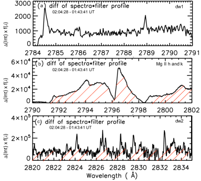
Figure 10: Variation with the wavelength of the difference of intensity between flare and preflare times in three wavelength ranges containing continuum regions (dw1 and dw2) and Mg II h $\&$ k line. The differences of intensity have been multiplied by the transmission filter profile f($\lambda$) of the 2832 Å filter ((Kleint et al., 2017). After normalization of the hatched areas in panels (b and c), we estimate that the contribution of the excess of the Balmer emission is 82 % compared to the contribution of the Mg II k line around 18$\%$ in the wavelength domain of the 2832 Å  SJI during the flare.

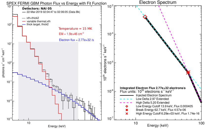
Figure 11: FERMI GBM photon spectra accumulated around 02:04:47 UT and 02:06:05 UT during the quoted 2-minute interval on March 22 2019 (left panel). Variable isothermal and thick target fitting done to the FERMI GBM spectrum. For variable thermal we use ‘vth’ function and for thick target we use ‘thick2’ from OSPEX. The variable thermal fit is shown by the red curve and the thick target fit is shown by the blue curve. The fit is limited between 8-30 keV shown by the shaded region. Above 30 keV counts are predominantly that of background. The fit shown here is best fit obtained using $\chi^{2}$ as a measure. We find a range of values for low-energy cutoff parameter (10.3 - 19.5 keV) gives reasonable fit. Electron spectrum given by the thick target fit is shown on the right panel.

4.2 Non-LTE radiative transfer models

The second step of our study was to estimate if the energy needed for the Balmer continuum excess could correspond to the energy brought by the bombardment of non thermal electrons. We need so to compare the energy input provided by non thermal electrons during the mini flare with the excess of the Balmer continuum enhancement observed by IRIS. This kind of comparison was done previously in the paper of Kleint et al. (2016) where they presented IRIS and RHESSI data for a strong X-ray flare. For that the former authors considered a theoretical grid of 1D static flare atmosphere models developed by Ricchiazzi & Canfield (1983), usually referred as RC models, in which the temperature structure is computed via the energy-balance between the electron-beam heating, conduction and net radiation losses and using as a free parameter the enhancement of the coronal pressure due to evaporation. Further, Kleint et al. (2016) used the non-LTE code MALI to synthesize the hydrogen recombination continua for all the models. They compared the resulting intensities of the Balmer continuum to those detected by IRIS. The RC flare models thus provide a relationship between the electron-beam energy flux with the cut-off energy 20 keV having a given spectral index and the enhancement of the Balmer continuum. Our observed excess of the Balmer continuum intensity is of the order of 1.5 to 1.75 $\times$ 10⁵ erg s^-1 sr^-1 cm^-2 Å^-1 (Fig. 6 panels g and h, Fig. 10 panel c). According to results of Kleint et al. (2016) (see their Table 1) this value is roughly consistent with a beam flux of 10⁹ and 10¹⁰ erg s^-1 cm^-2 (RC models E5 and E12). Such fluxes have been derived from FERMI GBM observations as we show above. For model E5 the coronal pressure is 100 dyn cm^-2 which leads to very bright Mg II line cores as computed in Liu et al. (2015) which are not observed in our weak flare (such a high pressure is found in an X-class flare atmosphere analyzed by Liu et al. (2015). The second model E12 with lower coronal pressure predicts the Mg II line-core intensities more compatible with our IRIS observations and is thus reasonable for this weak flare. The energy value is of same order than the energy brought by the electron beams of FERMI GBM between 10⁹ and 10¹⁰ erg s^-1 cm^-2 due to the uncertainty of the area size.

5 Discussion and conclusion

We extend the analysis of the IRIS data of GOES B6.7 micro flare (or mini flare) observed on March 22, 2019 focusing on the IRIS SJIs in the 2832 Å filter and the NUV continuum spectral variation in the two extreme wavelength domains of the IRIS 2896 Å spectra bandpass (between 2784-2791.5 Å and 2827-2834.5 Å). The mini flare and its site of reconnection identified by bidirectional outflows concern only one or two pixels along slit position 1 of the IRIS rasters (Joshi et al., 2021). Therefore we focus our analysis on the spectra along this slit. Through the paper we demonstrate that the enhancement of the NUV continuum was due to electron beams and not to the flare heating by inter-playing the analysis of IRIS images and spectra.

A brightening in the 2832 filter is visible in the area of the flare. After considering the wavelength domain of the filter, its transmission function, and the emission of the spectra in the same spectral domain we conclude that it was the direct signature of electron beams. In fact the excess of the Balmer continuum in the spectra detected at the flare time in the few considered pixels is constant all along the two considered spectral ranges (bottom panels of Fig. 6). The increment in the continuum intensity being constant can not be due to the intensity enhancement in the far wings of Mg II lines, which is decreasing with distance from the k (2796 Å) or h (2803 Å) Mg II line center on either side. Balmer continuum being optically-thin in a weak flare, thus its emission really far from Mg II h (more than 30 Å) for the second range is simply added to the photospheric (pre-flare) background as a constant excess of intensity over the photospheric continuum.

The co-temporal time of the continuum enhancement peak in the spectral profiles and in SJIs suggests that the SJI brigthness is dominated by the Balmer enhancement continuum. We found that the contribution of the Balmer continuum is of the order of 82 % compared to the 18 % of the extended Mg II line wings in the spectra domain of the 2832 filter. Besides the NUV continuum in this wavelength range is relatively simple to analyse, because the metallic lines (mainly Fe II lines) present in this domain are not in emission for this mini flare. This is a very different case from previous studies concerning X-class flares where metallic lines in the spectra around 2830 Å  went into emission and affected the Balmer continuum (Heinzel & Kleint, 2014; Kleint et al., 2017). The previous authors had to disentangle between the two emissions: continuum and Fe II lines.

For our weak flare we demonstrate that the FERMI GBM energy output by non thermal electrons is consistent with the beam flux required in non-LTE radiative models for getting the Balmer continuum emission excess measured in the IRIS spectra. In large flares, it has been shown that the injected non thermal energy derived from RHESSI data is sufficient and even in excess for explaining the thermal component of strong flares (Aschwanden et al., 2017; Kleint et al., 2016). However it was shown that for weak flares there was a deficit of energetic electrons for affecting the low levels of the atmosphere where the bolometric emission (NUV, White-light, near IR radiation) is initiated (Warmuth & Mann, 2020). Inglis & Christe (2014); Warmuth & Mann (2020) notice an apparent deficit of non thermal electrons in weak flares by computing the ratio between thermal energy (and losses) and energy in non thermal electrons. The interpretation depends on where and in which area the electrons are accelerated. In the strong energetic flares studied by Heinzel & Kleint (2014), and Kleint et al. (2017) the electron beam energy was large enough to power the thermal flare as the Ricchiazzi & Canfield (1983) models demonstrated.

In our case the reconnection site of the mini flare at the base of the jet has been identified in a tiny bald patch region transformed dynamically in a X-point current sheet which explains its multi-thermal components (Joshi et al., 2020). The electron beam input should be sufficient to power the thermal flare observed with Balmer continuum excess. The estimation of the non thermal energy is based on the size of the deposit electron area. This is a relatively unknown variable. The site of reconnection may be smaller than the IRIS spatial resolution and the energy input per unit area is may be underestimated. The spectral signatures of the mini flare have been identified as IRIS bomb spectra (Peter et al., 2014; Grubecka et al., 2016; Young et al., 2018; Joshi et al., 2021). Such structures can be due to plasmoid instablity which creates tiny multi-thermal plasmoids not resolved by our telescopes (Ni et al., 2016; Baty, 2019; Ni et al., 2021).

This study shows that the non-thermal HXR emission detected by FERMI GBM is strongly related to the enhancement of the Balmer continuum emission, signature of a significant excess of heating, therefore we conclude that the detection of the Balmer continuum emission in our mini flare supports the scenario of hydrogen recombination in flares after a sudden ionization at chromospheric layers.