Accelerated MRI Reconstruction with Separable and Enhanced Low-Rank Hankel Regularization
Abstract
The combination of the sparse sampling and the low-rank structured matrix reconstruction has shown promising performance, enabling a significant reduction of the magnetic resonance imaging data acquisition time. However, the low-rank structured approaches demand considerable memory consumption and are time-consuming due to a noticeable number of matrix operations performed on the huge-size block Hankel-like matrix. In this work, we proposed a novel framework to utilize the low-rank property but meanwhile to achieve faster reconstructions and promising results. The framework allows us to enforce the low-rankness of Hankel matrices constructing from 1D vectors instead of 2D matrices from 1D vectors and thus avoid the construction of huge block Hankel matrix for 2D k-space matrices. Moreover, under this framework, we can easily incorporate other information, such as the smooth phase of the image and the low-rankness in the parameter dimension, to further improve the image quality. We built and validated two models for parallel and parameter magnetic resonance imaging experiments, respectively. Our retrospective in-vivo results indicate that the proposed approaches enable faster reconstructions than the state-of-the-art approaches, e.g., about faster than STDLR-SPIRiT, and faithful removal of undersampling artifacts.
Index Terms:
Parallel imaging, parameter imaging, image reconstruction, Low-rank Hankel matrixI Introduction
Magnetic resonance imaging (MRI) is a non-radioactive, non-invasive imaging technique that is able to provide multi-contrast images and permit excellent soft-tissue images. It has become an indispensable tool in medical diagnosis. However, the long acquisition time is one of its prominent limitations, which may introduce motion-caused artifacts into the images and may not be practical in some application scenarios [1].
To alleviate the prolonged acquisition time, researchers have made great efforts. Shortening the scan time by acquire only a small subset of the k-space data has emerged as an effective and widely-used way [2, 3]. The sparse sampling technique enables significant reduction of time, but results in undersampling artifacts in the images due to sub-Nyquist sampling. Therefore, reconstruction models with prior information are exploited to enable promising results. Sparsity, low-rank, and sparsity plus low-rank are commonly-used priors. For instance, the sparse MRI methods enforce the sparsity of images in the transform domain, e.g., total variation [4], wavelets [2], contourlets [5], and adaptive sparse transform [6, 7, 8, 9, 10, 11]. The low-rank prior stems from the linear correlations among multiple MRI images [3], such as, dynamic MRI [12, 13], parameter imaging [14, 15], and high-dimensional MRI [16, 17] and has been utilized.
The low-rank structured matrix prior has been shown to be able to permit promising results [18, 19, 20, 21, 22]. For instance, simultaneous autocalibrating and k-space estimation [19] utilizes the strong correlation among receiver coils to enable the low-rankness of a block Hankel matrix constructed from the multi-coil k-space data. The low-rank matrix modeling of local k-space neighborhoods (LORAKS) [18] assumes the image of interest has limited support and/or a slowly varying phase, which would lead to a block-Hankel-like matrix being low-rank. The annihilating filter-based low-rank Hankel matrix approach (ALOHA) [20], and Ongie’s method [21] consider the sparsity of the signal in the transform domain. Similarly, the simultaneous two-directional low-rankness with SPIRiT (STDLR-SPIRiT) method [22] exploits the low-rank prior and enforces the self-consistency of k-space data providing state-of-the-art performance.
The structured low-rank methods lift the signal into a higher dimensional space to achieve low-rankness. However, the lifting brings some limitations, such as, large memory consumption and lengthy computational time. As for four-coil data, the dimension of its block Hankel matrix reaches when the pencil parameters equal . Researcher have established methods aiming to tackle the problem. The generalized iterative reweighted annihilating filter algorithm [23] utilized the convolutional structure of the lifted matrix so that it can performs the computations in the original signal instead of the lifted matrix. This method dramatically reduces the complexity and shortens the computational time. Auto-calibrated-LORAKS (AC-LORAKS) [24] exploited the auto-calibration signal (ACS) to reduce the computational time. Though the two methods gain considerable acceleration in time, they take advantage of specific priors that may not available in other low-rank approaches. Thus, fast low-rank Hankel MRI reconstruction is still highly desirable.
In this work, we attempted to establish a framework to permit fast and reliable low-rank reconstructions. A separable low-rank reconstruction method was proposed by enforcing the low-rankness of multiple small Hankel matrices from each row and each column of MRI data, avoiding constructing the high-dimensional low-rank matrix thereby enables much less memory and allows faster computation. In addition, the self-consistence and conjugate symmetric of k-space data are considered to further reduce the reconstruction error. Besides, the parameter-dimensional information will be introduced into formulation so that the original model can not only be applied to non-parameter parallel imaging but also extended to parameter imaging. The proposed method is expected to effectively utilize the low-rank property to yield fast reconstruction and maintain low reconstruction error.
The rest of this paper is organized as follows. We introduce some notations in Section II, and related work in Section III. Section IV presents the proposed model and numerical algorithm for non-parameter and parameter parallel imaging reconstructions, and Section III demonstrates the reconstruction performance. Section VI discusses some factors that may affect the reconstruction error and speed. The conclusions are finally drawn in Section VII.
II Notations
For easier reading, we first list some notations used throughout this paper in Table I.
| Symbol | Quantity |
|---|---|
| desired multi-coil k-space data, (rows) (columns) (coils) | |
| desired multi-coil image, (rows) (columns) (coils) | |
| vector of the -th row and the -th coil of | |
| vector of the -th column and the -th coil of | |
| desired image of parameter imaging , (FE) (PE) (P) (coils) | |
| desired image at the -th position on FE dimension of parameter imaging, (PE) (P) (coils) |
-
•
Note: the FE is the abbreviation of frequency encoding, the PE is the abbreviation of phase encoding, the capital letter P denotes the parameter dimension.
III Related Work
The STDLR [22] simultaneously enforced the low-rank constraint of k-space data along both horizontal and vertical directions as follows:
| (1) |
where denotes the targeted k-space data, and the acquired multi-coil k-space data with zero-filling in unacquired position. The operator transfers multi-coil data into a cascaded block Hankel matrix; and are weighting operators that perform weighting on k-space data of each coil image, whose weights are the Fourier transform of filters in the horizontal and vertical directions; represents an operator that undersamples data, and means arranging a matrix or a tensor to a vector.
The STDLR explored the simultaneous horizontal and vertical directional low-rankness in the k-space data, reducing the image reconstruction errors. Compared to the state-of-the-art method ALOHA, STDLR achieves lower reconstruction errors [22]. However, the size of the block Hankel matrix appears dramatically huge, leading to a long computational time and large memory requirements. Take four-coil parallel imaging data for an example, the STDLR requires s to finish reconstruction while the separable Hankel low-rank method takes only s (Fig. 2).
IV Proposed Method
IV-A Basic Model - SHLR
In this work, we first proposed a separable Hankel low-rank reconstruction method (SHLR) to enforce the low-rankness of Hankel matrices constructing from each row and each column as follows:
| (2) |
where the denotes the desired multi-coil image, is the 2D Fourier transform for each coil data. The and denote the operators that extract -th row (-th vector on the first dimension) and -th column (-th vector on the second dimension) from each coil data for and . Here, we define as the -th row and -th coil of , and as the -th column and -th coil of . Then, we have and .
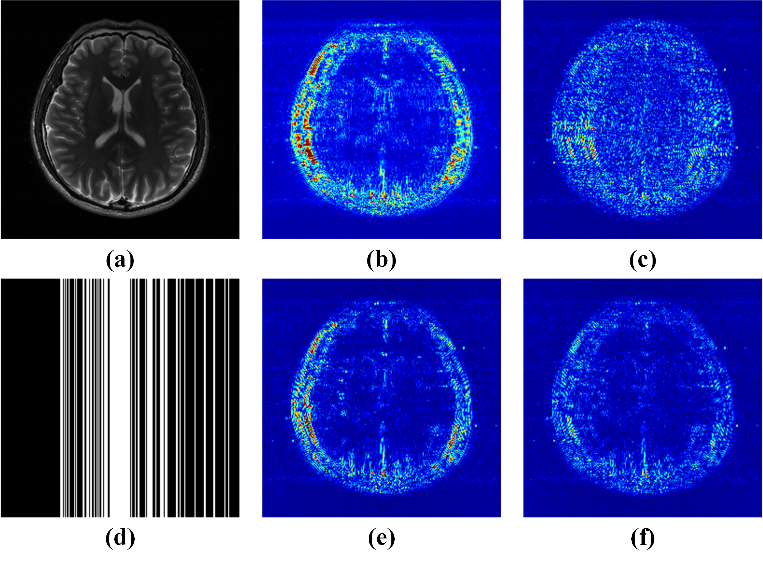
Fig. 3 shows a graphical illustration of the notations of constructing Hankel matrices. The operator denotes the 1D Fourier transform on a vector, performs weighting on a vector with the weights obtained from applying Fourier transform to 1D sparse transform filter, and converts a vector into a Hankel matrix. The tilde above the operator means that corresponding operation is performed on each column vector of the matrix, that is and .
IV-B Enhanced Model
As mentioned above, building the block Hankel matrix requires huge memory consumption and thereby increases the computational complexity and time. To mitigate the problem, we proposed to establish multiple small-size Hankel matrices by exploiting the low-rankness of a row or a column vector of the signal. This will significantly reduce memory consumption and make computational speed much faster.
However, constraining the low-rankness of each row and each column separately weakens the utilization between rows and columns, leading to an increase in reconstruction errors, e.g. relative norm error (RLNE). (Fig. 2 (e-f)). In order to improve the reconstruction while maintaining a faster reconstruction speed, we consider introducing other information to strengthen the constraints of the model. The following three kinds of information are exploited.
IV-B1 Strengthen the correlation between rows and columns
The proposed SHLR method makes little use of the correlation between rows and columns. A natural idea for improvement is to strengthen the exploitation of k-space neighborhood information. The SPIRiT is a good choice. The SPIRiT [25] primarily bases on the assumption that each k-space data point is the convolution of multi-coil data of its neighboring k-space, which implies the SPIRiT constraint has the ability to utilize the linear correlation of adjacent rows and columns to reconstruct MRI image. Therefore, the SHLR with SPIRiT constraint (SHLR-S) can be modeled as:
| (3) |
where denotes the SPIRiT operator in image domain.
IV-B2 Strengthen the low-rankness within each row (or column)
Another way to improve the reconstruction is to strengthen the low-rankness within each row and each column. The smooth phase of MRI images is often used as prior information to be involved in MRI reconstruction [26, 27, 18]. By generating the virtual coils containing the conjugate symmetric, the smooth MRI image phase information can be incorporated into the reconstruction problem [28]. The conjugate symmetry of k-space has been applied into the Hankel low-rank reconstruction [29]. This property can be easily introduced into SHLR reconstruction model as:
| (4) |
where the superscript represents the operation of taking the conjugate and flipping the vector along the center. Therefore, we can formulate the SHLR with virtual coil (SHLR-V) as:
| (5) |
We introduced both the SPIRiT and virtual coil information into the basis SHLR model aiming to further reduce the reconstruction errors. We can achieve better reconstruction results with the optimization as:
| (6) |
As shown in Fig. 4, the SHLR-SV, which equipped with both the SPIRiT and virtual coil information, produces the image with lowest error (Fig. 4 (f)) while the basic SHLR and the SHLR with only one extra information enforcement yield results with obvious errors (Fig. 4 (b-c) and (e)). The results indicate the effectiveness of utilizing the two information in parallel imaging.
IV-B3 Parameter-dimensional information
Extra information can be incorporated to improve reconstructions of multi-dimensional MRI, e.g., information from parameter imaging.
Conventional parameter imaging acquires a series of images using different parameters. The image intensity variation along the parameter dimension then is used in data fitting to estimate the tissue intrinsic parameters, such as longitudinal relaxation time (T1), transversal relaxation time (T2). The tissue parameters are important in diagnosing the diseases including nervous, musculoskeletal, liver, and myocardial [30, 31, 32, 33, 34, 14]. It is worthy to mention that the signal along the parameter dimension can be modeled as mono or few exponentials [31, 34, 35], which indicates the low-rankness of the signal [15, 35, 36]. The low-rank property along the parameter dimension can be utilized to enhance the reconstructions.
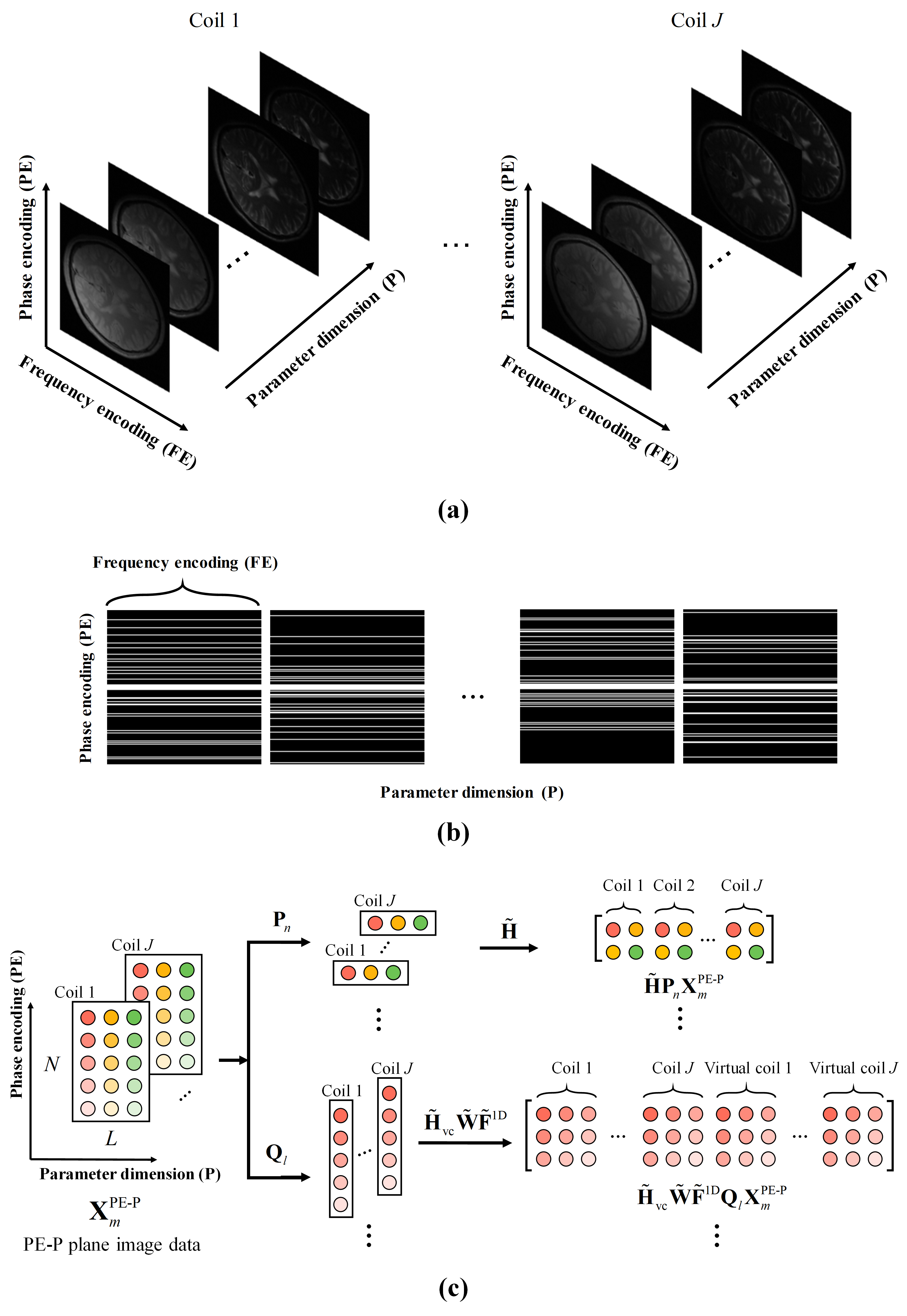
Motivated by ALOHA [35], we reconstruct images in the frequency encoding dimension one-by-one (Fig. 5). The difference between ALOHA and our proposed method is that ALOHA constructed a block Hankel matrix from the data on the phase encoding-parameter (PE-P) plane while the proposed method converted rows or columns on the phase encoding-parameter plane into Hankel matrices separately. The seperable low-rank Hankel matrix strategy reduces the reconstruction time to a certain extent (Fig. 6).
Let denote the desired parameter imaging MRI image. Denote as the image at the -th position on the frequency encoding dimension of . Let denote the acquired k-space data of parameter imaging, with zero-filling at unacquired position and 1D inverse Fourier transform on along the frequency encoding dimension. And let represent the data at the -th position on the frequency encoding dimension of . denotes the 1D Fourier transform along the phase encoding dimension. The reconstruction model for parameter imaging is as follow
| (7) |
To further reduce the reconstruction error, we establish a reconstruction approach that takes advantages of both virtual coil and parameter-dimension information. Notice that SPIRiT exploits the correlation of image of different coils, it appears not appropriate for the recovery of PE-P plane images. Thus, the proposed method stems from the basic model and introduces two prior information, smooth phase of the image and low-rankness in the parameter dimension:
| (8) |
As shown in Fig. 6, the SHLR-VP which utlizes the virtual coil acheives the lowest error, and the computational time of the proposed SHLR-VP is reduced to of that of ALOHA. The results demonstrate the advantages of the proposed method in terms of low reconstruction error and fast reconstruction speed for parameter imaging.
IV-C Numerical Algorithm
We adopted the alternating direction method of multiplier (ADMM) [37] to solve both the proposed SHLR-SV in Eq. (6) and the SHLR-VP model in Eq. (8).
IV-C1 SHLR-SV
The augmented Lagrangian form of Eq. (6) lies in
| (9) |
where represents the inner product of matrix, and the penalty parameter.
The solution of Eq. (9) can be obtained by alternatively solving the following sub-problems:
| (10) |
| (11) |
| (12) |
| (13) |
| (14) |
where is the step size.
For fixed , , , and , has a close-form solution as
| (15) |
where the upper subscript denotes the adjoint operator. Here, for any matrix , , therefore, we omitted the writing of for simplicity in the following.
For fixed and , is obtained by
| (16) |
where denotes the singular value threshold operator with the threshold of .
Similarly, the can also be obtained by
| (17) |
The numerical algorithm for SHLR-SV is summarized in Supplementary Material S1.
IV-C2 SHLR-VP
Considering the space limitations, please refer to Supplementary Material S2 for detailed derivations for solving the SHLR-VP model.
V Results
In this section, we will evaluate the two proposed approaches, SHLR-SV and SHLR-VP using in vivo data from different MRI scanners.
In all experiments, the multi-coil images are combined by a square root of squares (SSOS). We adopted the RLNE [38] and mean structure similarity index measure (MSSIM) [39] as objective criteria to quantify the reconstruction performance. A lower RLNE, the higher consistency lies between the fully sampled image and the reconstruction image. A higher MSSIM indicates higher detail preservation in reconstruction. The calculation of RLNE and MSSIM can be found in Supplementary Material.
V-A Parallel Imaging
In this subsection, we assessed the reconstruction results and running time of SHLR-SV and compared the results of SHLR-SV with three state-of-the-art reconstruction approaches including -SPIRiT [25], AC-LORAKS [24], and STDLR-SPIRiT [22]. These three methods and SHLR-SV require ACS for reconstruction. More specifically, -SPIRiT reconstructs image by exploiting kernel estimation and the sparsity of the image in the transform domain. Both AC-LORAKS and STDLR-SPIRiT utilize the low-rankness of block Hankel matrix (or structured matrix) of k-space to recover MRI image. In addition, AC-LORAKS utilizes ACS for reducing the algorithm complexity [24].
The codes of -SPIRiT are shared online by Dr. Michael Lustig [40] and codes of AC-LORAKS [41] are shared at Dr. Justin P. Haldar’s website. Here, we adopted the S-based AC-LORAKS with virtual coil which makes use of phase constraints. The reason why we chose S-based is that LORAKS with phase constraint provides results with lower error compared to other constraints [18]. Parameters of all the compared methods are optimized to obtain the lowest RLNE. For the proposed methods, the effect of parameters setting will be discussed in Supplementary Material S5.
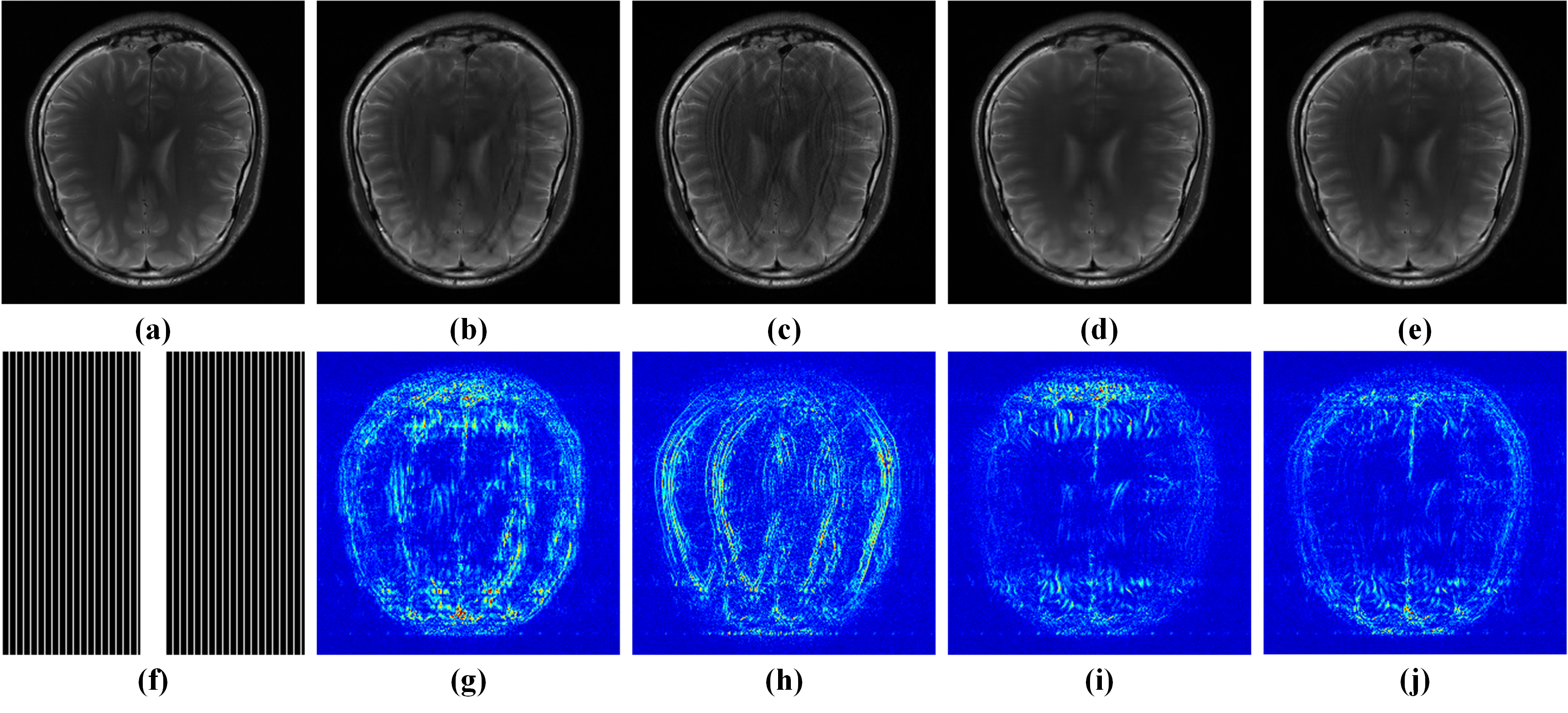
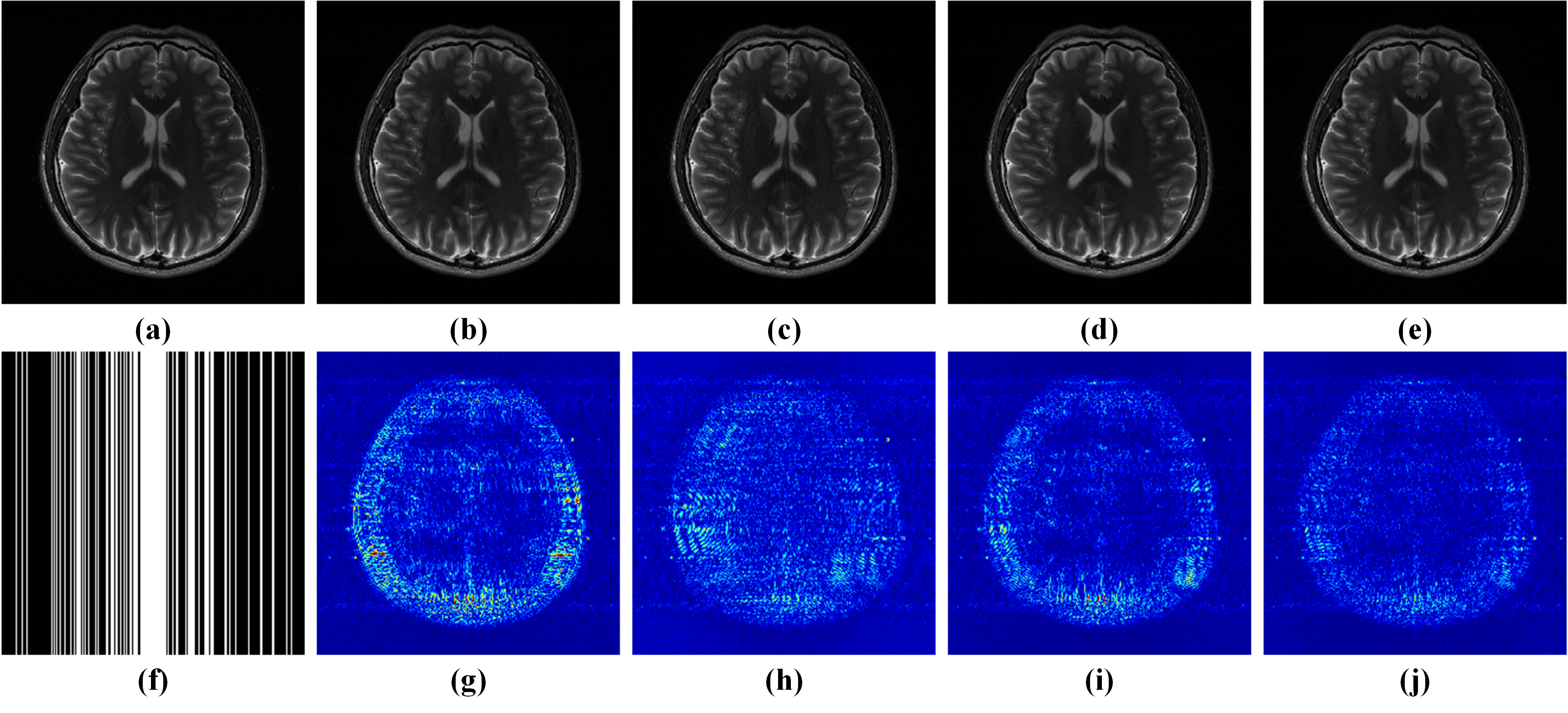
Two brain datasets acquired from healthy volunteers are adopted in experiments. The dataset depicted in Fig. 7 (a) is obtained from a 3T SIEMENS MRI scanner (Siemens Healthcare, Erlangen, Germany) equipped with 32 coils using T2-weighted turbo spin echo sequence (matrix size = , TR/TE = ms, FOV = mm mm, slice thickness = mm). Eight virtual coils are compressed from the acquired data of 32 coils [42] to reduce the computational complexity. The other dataset shown in Fig. 8 (a) is acquired from a 3T SIEMENS Trio whole-body scanner (Siemens Healthcare, Erlangen, Germany) equipped with 32 coils using the 2D T2-weighted turbo spin echo sequence (matrix size = , TR/TE = ms, FOV = mm mm, slice thickness = mm). Four virtual coils are compressed from the acquired data of 32 coils [42].
We first test the proposed method for parallel imaging using the widely-used sampling pattern adopted in commercial MRI scanners named uniform undersampling pattern. Both -SPIRiT (Fig. 7 (b)) and AC-LORAKS (Fig. 7 (c)) have strong undersampling artifacts. STDLR-SPIRiT (Fig. 7 (d)) and SHLR-SV (Fig. 7 (e)) show the good ability of artifacts removing. But it is worthy to note that SHLR-SV provides the image with lower error than STDLR-SPIRiT.
We then test the proposed method using non-uniform undersampling patterns, including 1D Cartesian and 2D random undersampling patterns. In the reconstruction under Cartesian undersampling pattern, AC-LORAKS (Fig. 8 (c)) yields results exhibiting obvious artifacts inside the brain area, whereas the ringing artifacts also remain in the reconstructed image of -SPIRiT (Fig. 8 (b)). Both STDLR-SPIRiT (Fig. 8 (d)) and SHLR-SV (Fig. 8 (e)) provide the image with nice artifacts suppression, however, the reconstruction error of STDLR-SPIRiT appear slightly larger than that of SHLR-SV, especially in the skull area.
| Image | -SPIRiT | AC-LORAKS | STDLR-SPIRiT | SHLR-SV |
|---|---|---|---|---|
| Fig. 7 | 0.0688/0.9637 | 0.0709/0.9386 | 0.0488/0.9810 | 0.0482/0.9822 |
| Fig. 8 | 0.0689/0.9856 | 0.0596/0.9806 | 0.0518/0.9918 | 0.0426/0.9934 |
| Fig. 9 | 0.1028/0.9751 | 0.0935/0.9543 | 0.0914/0.9833 | 0.0639/0.9882 |
In addition, SHLR-SV allows promising reconstruction on the undersampling patterns with partial Fourier (PF), which is commonly adopted in commercial equipment for further acceleration [26], indicating the potential to be robust to patterns. As shown in Fig. 9, under the case with PF, the reconstruction errors of three compared approaches, including STDLR-SPIRiT, apparently increased, whereas SHLR-SV still yields nice reconstruction with low reconstruction error. In the meanwhile, the proposed SHLR-SV outperforms other methods in terms of RLNE and MSSIM, indicating the excellent ability of artifact suppression and detail preservation.
We include more data and sampling patterns to further evaluate the proposed SHLR-SV approach. The detailed results can be found in Supplementary Material S3. Similar phenomenons were observed in the results indicating SHLR-SV is robust to the different data from different subjects, and also robust to different sampling patterns. It can be seen that SHLR-SV outperforms the -SPIRiT and AC-LORAKS, and shows comparable results with STDLR-SPIRiT. Given the patterns with PF, SHLR-SV gains a slight improvement than STDLR-SPIRiT with respect to RLNE and MSSIM. However, the computational time of the proposed method is significantly reduced compared to that of STDLR-SPIRiT ( faster). Overall, the proposed method provides faithful reconstruction with acceptable computational time, having the potential to be used in clinical applications.
V-B Parameter Imaging
In this subsection, we validate the proposed SHLR-VP method using a acquired in-vivo T2 mapping data. We compare the proposed method named SHLR-VP with two state-of-the-art mapping reconstruction methods including MORASA [15], and ALOHA [35]. These two methods both utilized the property of exponential in the parameter dimension. MORASA modeled the time-domain signal into a exponential function and the enforced the sparsity of the image at each time point. ALOHA made use of the annihilation relationship of the data and lifted the signal into a higher dimensional space to ensure the low-rankness. The codes of MORASA are shared by Dr. Xi Peng and codes of ALOHA [43] are shared at Dr. Jong Chul Ye website.
A fully sampled brain dataset was acquired from a healthy volunteer on a 3T 12 coils MRI scanner (Siemens Healthcare, Erlangen, Germany) using turbo spin echo sequence (TR = ms, TEs from to ms with ms sapcing, FOV = mm mm, matrix size = , slice thickness = mm). To estimate the T2 map, standard nonlinear least square fitting method was performed in the selected region-of-interest on a pixel-by-pixel basis. T2 relaxation values outside the reasonable range were excluded from the T2 map.
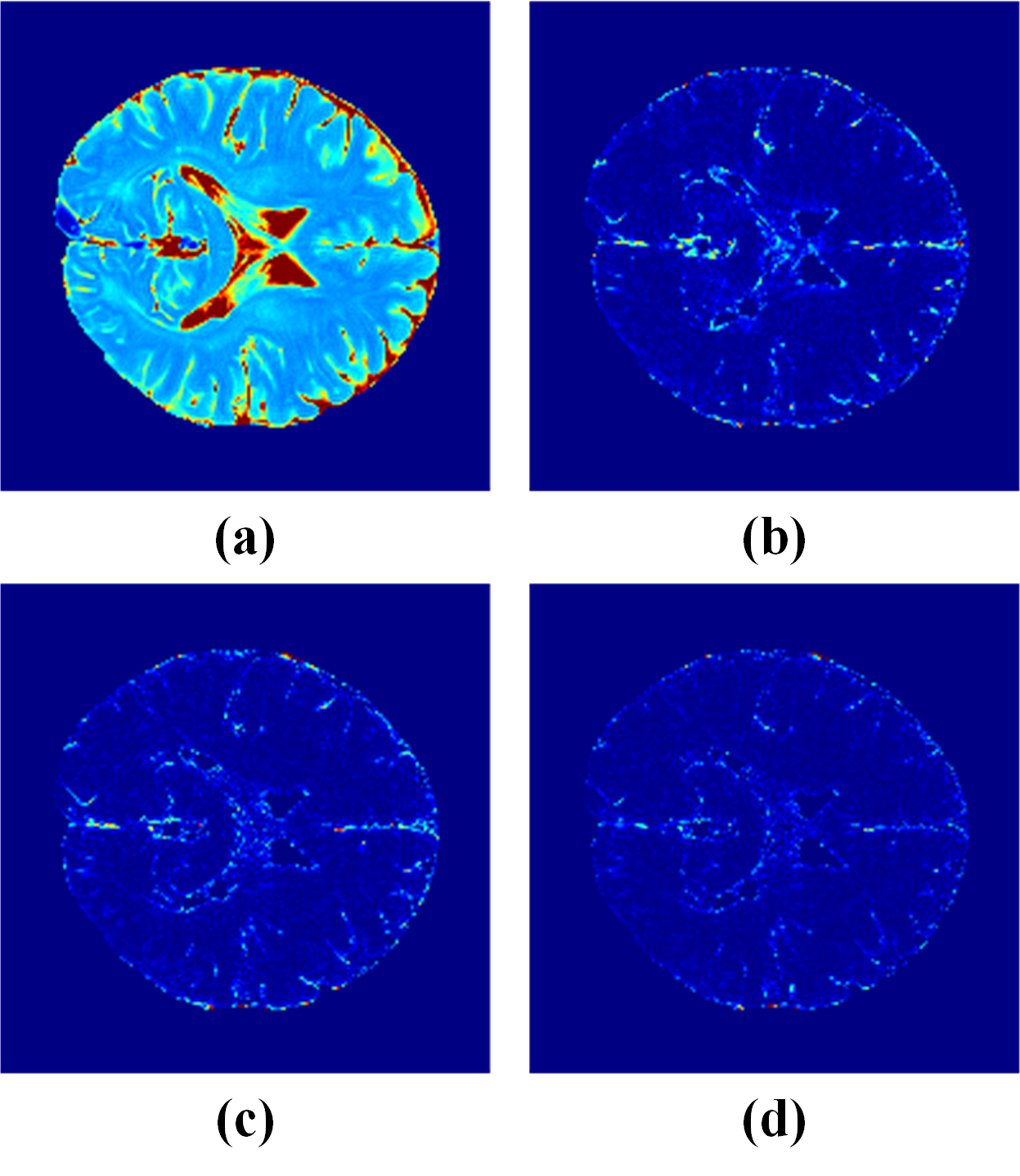
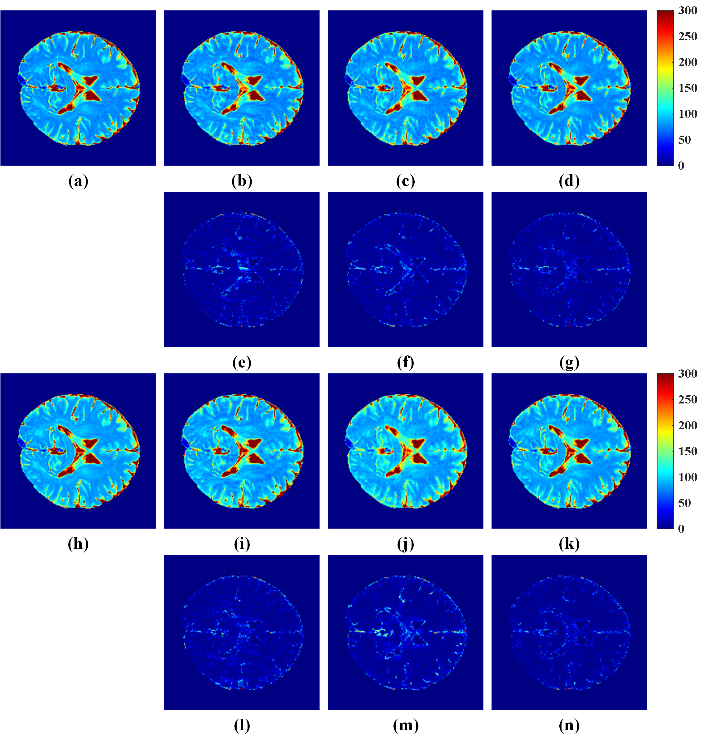
We performed reconstructions under two different reduction factors, and . In both cases, the MORASA images appear apparent string-like artifacts (Fig. 10 (e) and (i)). Compared to ALOHA, SHLR-VP produces mapping results with better accuracy. As can be seen from the images, the mapping error is obviously smaller than that of ALOHA. The RLNE and MSSIM also indicate that SHLR-VP persevere the image structure better than the comparison methods.
In addition, we validated the proposed method using other datasets, and the sampling patterns with PF. Please refer to the Supplementary Material S4 for detailed results. The results demonstrate that the proposed method SHLR-VP yields reconstructions with the lowest error in both reconstructed images and the quantization T2 map.
VI Discussions
VI-A The Number of ACS
The ACS is crucial for traditional parallel reconstruction methods. These methods estimate sensitivity maps or kernels from ACS, once the number of ACS lines is limited, the estimation turns inaccurate, leading to failures of reconstruction [19]. Four comparison methods for parallel imaging require ACS to reconstruct images, thus, in this subsection we discuss the effect of the number of ACS on the reconstructed results.
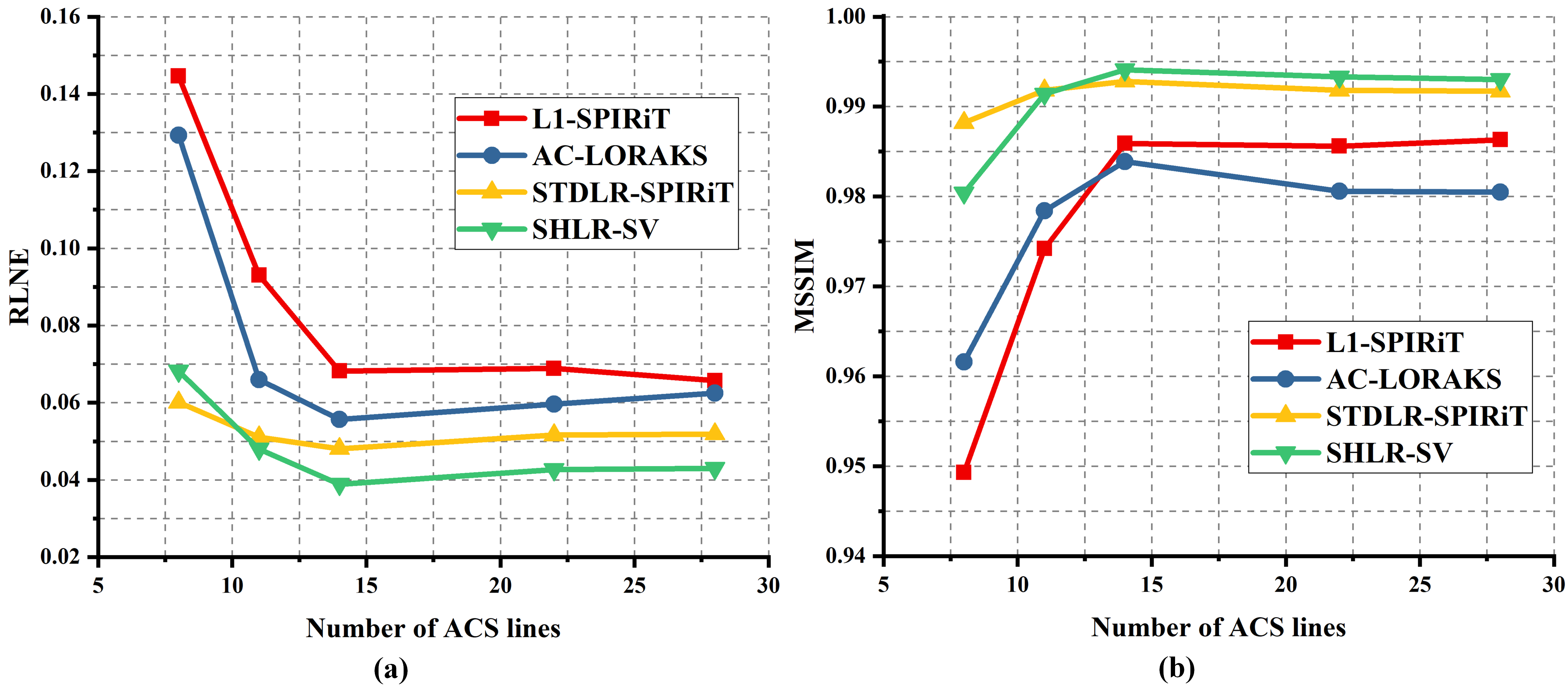
The results shown in Fig. 11 indicates the proposed SHLR-SV maintains the robustness to ACS lines. When ACS lines ( lines) are relatively sufficient, all these comparison methods provide reconstruction with relatively low reconstruction error. Especially, the proposed method SHLR-SV achieved the lowest RLNE and the highest MSSIM. However, when the number of ACS lines is extremely low (), -SPIRiT and AC-LORAKS fail to produce satisfying results (the RLNE reaches closely to ). In contrast, the STDLR-SPIRiT and SHLR-SV, still work well, even with only ACS lines offering an RLNE of approximately 0.07. The observation demonstrates that the proposed SHLR-SV still inherits the robustness of structured low-rank methods.
VI-B Computational Time
All reconstruction software were ran on a CentOS 7 computation server with two Intel Xeon CPUs of 3.5 GHz and 112 GB RAM. The computational time is obtained by averaging the reconstruction time of Monte Carlo tests. All comparison approaches were implemented in MATLAB.
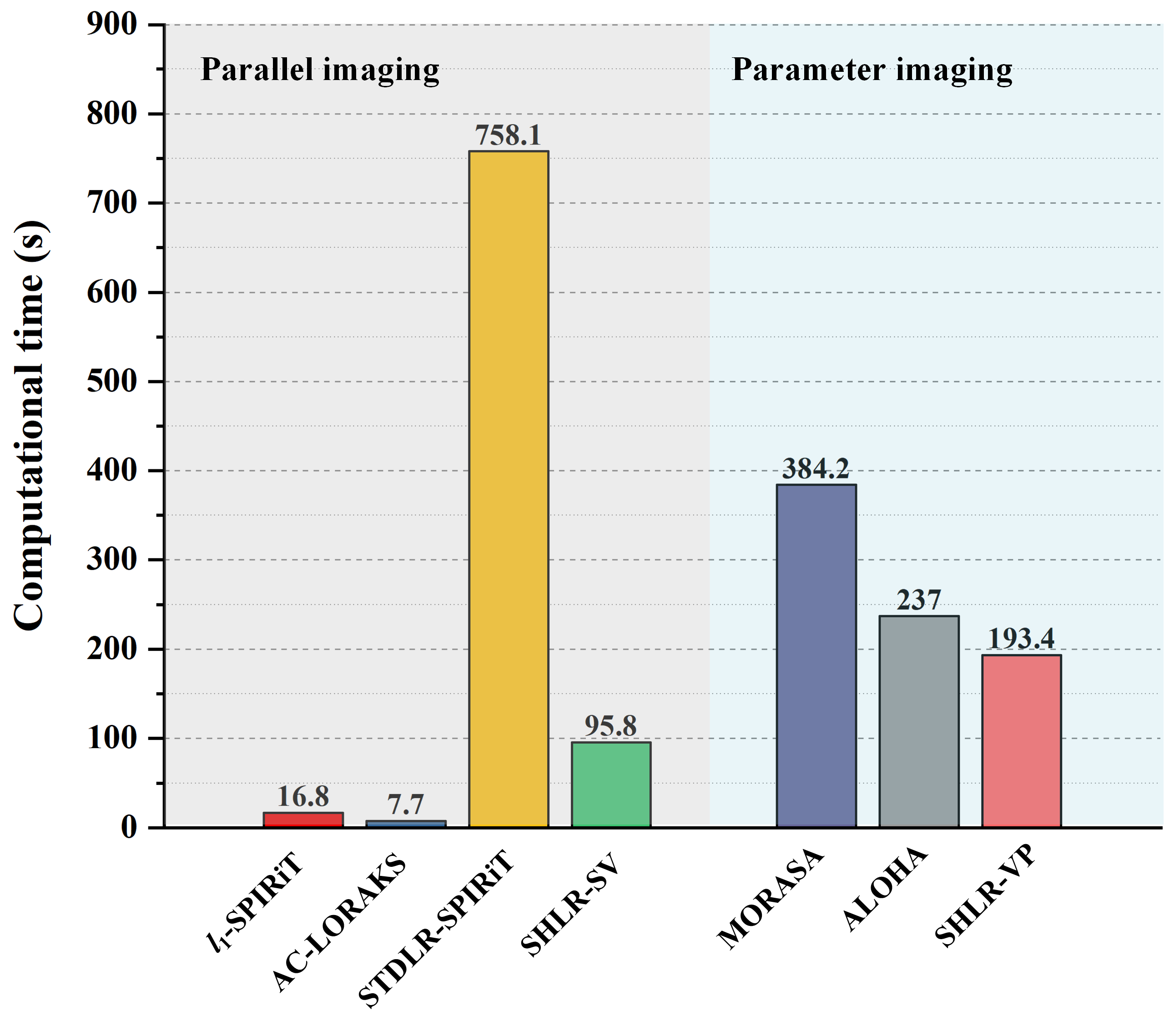
As shown in Fig. 12, the running time of SHLR-SV is reduced to of that of STDLR-SPIRiT, which substantially alleviates the burden of lengthy reconstruction time of STDLR-SPIRiT. Moreover, it can be observed that the proposed method runs relatively slower than -SPIRiT and AC-LORAKS. However, the additional computational cost of SHLR-SV should be acceptable considering its improvement in image reconstruction.
The computational time on parameter imaging reconstruction is also depicted in Fig. 12. It shown that the proposed SHLR-VP reconstructs data at a faster speed than MORASA and ALOHA. Besides, it is worthy to notice that runtime of the proposed method can be further reduced with GPU or MEX/C implementations.
VII Conclusion
In this work, we attempted to alleviate the huge computational complexity and lengthy reconstruction time problems of the state-of-the-art structural low-rank approaches. To reduce the computational time, we proposed a separable Hankel low-rank reconstruction method, named SHLR, to enforce the Hankel low-rankness of each row and each column of the signal of interest. But this way to enforce the low-rankness is sub-optimal compared to block Hankel methods, though holds the advantage of swift runtime. To enhance the performance of SHLR, we introduced prior information. For parallel imaging, we explored the correlation between rows/columns and the virtual coil technique, and proposed the SHLR-SV model. Regarding parameter imaging, we assumed that the signal intensity along the parameter dimension varies in an exponential way. We enforced the exponential property and virtual coil technique and proposed a model named SHLR-VP for accelerating parameter imaging.
Experimental in-vivo results showed that the proposed two approaches enable better results than the state-of-the-art methods. Notably, the proposed methods allow reconstructions with smaller errors and faster reconstruction speed.
References
- [1] J. Hamilton, D. Franson, and N. Seiberlich, “Recent advances in parallel imaging for MRI,” Progress in Nuclear Magnetic Resonance Spectroscopy, vol. 101, pp. 71–95, 2017.
- [2] M. Lustig, D. Donoho, and J. M. Pauly, “Sparse MRI: The application of compressed sensing for rapid MR imaging,” Magnetic Resonance in Medicine, vol. 58, no. 6, pp. 1182–1195, 2007.
- [3] Z. Liang, “Spatiotemporal imaging with partially separable funcrions,” in 2007 4th IEEE International Symposium on Biomedical Imaging: From Nano to Macro, 2007, Conference Proceedings, pp. 988–991.
- [4] K. T. Block, M. Uecker, and J. Frahm, “Undersampled radial MRI with multiple coils. Iterative image reconstruction using a total variation constraint,” Magnetic Resonance in Medicine, vol. 57, no. 6, pp. 1086–98, 2007.
- [5] X. Qu, W. Zhang, D. Guo, C. Cai, S. Cai, and Z. Chen, “Iterative thresholding compressed sensing MRI based on contourlet transform,” Inverse Problems in Science and Engineering, vol. 18, no. 6, pp. 737–758, 2010.
- [6] S. Ravishankar and Y. Bresler, “MR image reconstruction from highly undersampled k-space data by dictionary learning,” IEEE Transactions on Medical Imaging, vol. 30, no. 5, pp. 1028–1041, 2011.
- [7] X. Qu, Y. Hou, F. Lam, D. Guo, J. Zhong, and Z. Chen, “Magnetic resonance image reconstruction from undersampled measurements using a patch-based nonlocal operator,” Medical Image Analysis, vol. 18, no. 6, pp. 843–856, 2014.
- [8] Z. Zhan, J. Cai, D. Guo, Y. Liu, Z. Chen, and X. Qu, “Fast multiclass dictionaries learning with geometrical directions in MRI reconstruction,” IEEE Transactions on Biomedical Engineering, vol. 63, no. 9, pp. 1850–1861, 2016.
- [9] Z. Lai, X. Qu, Y. Liu, D. Guo, J. Ye, Z. Zhan, and Z. Chen, “Image reconstruction of compressed sensing MRI using graph-based redundant wavelet transform,” Medical Image Analysis, vol. 27, pp. 93–104, 2016.
- [10] S. Ravishankar and Y. Bresler, “Data-driven learning of a union of sparsifying transforms model for blind compressed sensing,” IEEE Transactions on Computational Imaging, vol. 2, no. 3, pp. 294–309, 2016.
- [11] Y. Liu, Z. Zhan, J.-F. Cai, D. Guo, Z. Chen, and X. Qu, “Projected iterative soft-thresholding algorithm for tight frames in compressed sensing magnetic resonance imaging,” IEEE Transactions on Medical Imaging, vol. 35, no. 9, pp. 2130–2140, 2016.
- [12] B. Zhao, J. P. Haldar, A. G. Christodoulou, and Z. Liang, “Image reconstruction from highly undersampled (k, t)-space data with joint partial separability and sparsity constraints,” IEEE Transactions on Medical Imaging, vol. 31, no. 9, pp. 1809–1820, 2012.
- [13] R. Otazo, E. Candes, and D. K. Sodickson, “Low-rank plus sparse matrix decomposition for accelerated dynamic MRI with separation of background and dynamic components,” Magnetic Resonance in Medicine, vol. 73, no. 3, pp. 1125–36, 2015.
- [14] T. Zhang, J. M. Pauly, and I. R. Levesque, “Accelerating parameter mapping with a locally low rank constraint,” Magnetic Resonance in Medicine, vol. 73, no. 2, pp. 655–661, 2015.
- [15] X. Peng, L. Ying, Y. Liu, J. Yuan, X. Liu, and D. Liang, “Accelerated exponential parameterization of T2 relaxation with model-driven low rank and sparsity priors (MORASA),” Magnetic Resonance in Medicine, vol. 76, no. 6, pp. 1865–1878, 2016.
- [16] X. Zhang, Z. Xu, N. Jia, W. Yang, Q. Feng, W. Chen, and Y. Feng, “Denoising of 3D magnetic resonance images by using higher-order singular value decomposition,” Medical Image Analysis, vol. 19, no. 1, pp. 75–86, 2015.
- [17] J. He, Q. Liu, A. G. Christodoulou, C. Ma, F. Lam, and Z. Liang, “Accelerated high-dimensional MR imaging with sparse sampling using low-rank tensors,” IEEE Transactions on Medical Imaging, vol. 35, no. 9, pp. 2119–2129, 2016.
- [18] J. P. Haldar, “Low-rank modeling of local k-space neighborhoods (LORAKS) for constrained MRI,” IEEE Transaction on Medical Imaging, vol. 33, no. 3, pp. 668–81, 2014.
- [19] P. J. Shin, P. E. Larson, M. A. Ohliger, M. Elad, J. M. Pauly, D. B. Vigneron, and M. Lustig, “Calibrationless parallel imaging reconstruction based on structured low-rank matrix completion,” Magnetic Resonance in Medicine, vol. 72, no. 4, pp. 959–970, 2014.
- [20] K. Jin, D. Lee, and J. Ye, “A general framework for compressed sensing and parallel MRI using annihilating filter based low-rank Hankel matrix,” IEEE Transactions on Computational Imaging, vol. 2, no. 4, pp. 480–495, 2016.
- [21] G. Ongie and M. Jacob, “Off-the-grid recovery of piecewise constant images from few fourier samples,” SIAM Journal on Imaging Sciences, vol. 9, no. 3, pp. 1004–1041, 2016.
- [22] X. Zhang, D. Guo, Y. Huang, Y. Chen, L. Wang, F. Huang, Q. Xu, and X. Qu, “Image reconstruction with low-rankness and self-consistency of k-space data in parallel MRI,” Medical Image Analysis, vol. 63, p. 101687, 2020.
- [23] G. Ongie and M. Jacob, “A fast algorithm for convolutional structured low-rank matrix recovery,” IEEE Transactions on Computational Imaging, vol. 3, no. 4, pp. 535–550, 2017.
- [24] J. P. Haldar, “Autocalibrated LORAKS for fast constrained MRI reconstruction,” in 2015 IEEE 12th International Symposium on Biomedical Imaging (ISBI), 2015, pp. 910–913.
- [25] M. Lustig and J. M. Pauly, “SPIRiT: Iterative self-consistent parallel imaging reconstruction from arbitrary k-space,” Magnetic Resonance in Medicine, vol. 64, no. 2, pp. 457–71, 2010.
- [26] D. Noll, D. Nishimura, and A. Macovski, “Homodyne detection in magnetic resonance imaging,” IEEE Transactions on Medical Imaging, vol. 10, no. 2, pp. 154–163, 1991.
- [27] F. Zhao, D. C. Noll, J.-F. Nielsen, and J. A. Fessler, “Separate magnitude and phase regularization via compressed sensing,” IEEE Transactions on Medical Imaging, vol. 31, no. 9, pp. 1713–1723, 2012.
- [28] M. Blaimer, M. Gutberlet, P. Kellman, F. A. Breuer, H. Köstler, and M. A. Griswold, “Virtual coil concept for improved parallel MRI employing conjugate symmetric signals,” Magnetic Resonance in Medicine, vol. 61, no. 1, pp. 93–102, 2009.
- [29] M. Mani, H. K. Aggarwal, V. Magnotta, and M. Jacob, “Improved MUSSELS reconstruction for high-resolution multi-shot diffusion weighted imaging,” Magnetic Resonance in Medicine, vol. 83, no. 6, pp. 2253–2263, 2020.
- [30] J. Warntjes, O. D. Leinhard, J. West, and P. Lundberg, “Rapid magnetic resonance quantification on the brain: Optimization for clinical usage,” Magnetic Resonance in Medicine, vol. 60, no. 2, pp. 320–329, 2008.
- [31] J. Sénégas, W. Liu, H. Dahnke, H. Song, E. K. Jordan, and J. A. Frank, “Fast T2 relaxometry with an accelerated multi-echo spin-echo sequence,” NMR in Biomedicine, vol. 23, no. 8, pp. 958–967, 2010.
- [32] A. L. Alexander, S. A. Hurley, A. A. Samsonov, N. Adluru, A. P. Hosseinbor, P. Mossahebi, D. P. Tromp, E. Zakszewski, and A. S. Field, “Characterization of cerebral white matter properties using quantitative magnetic resonance imaging stains,” Brain Connectivity, vol. 1, no. 6, pp. 423–446, 2011.
- [33] L. Feng, R. Otazo, H. Jung, J. H. Jensen, J. C. Ye, D. K. Sodickson, and D. Kim, “Accelerated cardiac T2 mapping using breath-hold multiecho fast spin-echo pulse sequence with k-t FOCUSS,” Magnetic Resonance in Medicine, vol. 65, no. 6, pp. 1661–1669, 2011.
- [34] B. Zhao, F. Lam, and Z.-P. Liang, “Model-based MR parameter mapping with sparsity constraints: Parameter estimation and performance bounds,” IEEE Transactions on Medical Imaging, vol. 33, no. 9, pp. 1832–1844, 2014.
- [35] D. Lee, K. H. Jin, E. Y. Kim, S.-H. Park, and J. C. Ye, “Acceleration of MR parameter mapping using annihilating filter-based low rank hankel matrix (ALOHA),” Magnetic Resonance in Medicine, vol. 76, no. 6, pp. 1848–1864, 2016.
- [36] M. Zimmermann, Z. Abbas, K. Dzieciol, and N. J. Shah, “Accelerated parameter mapping of multiple-echo gradient-echo data using model-based iterative reconstruction,” IEEE Transactions on Medical Imaging, vol. 37, no. 2, pp. 626–637, 2018.
- [37] S. Boyd, N. Parikh, E. Chu, B. Peleato, and J. Eckstein, “Distributed optimization and statistical learning via the alternating direction method of multipliers,” Foundations and Trends® in Machine Learning, vol. 3, no. 1, pp. 1–122, 2011.
- [38] X. Zhang, H. Lu, D. Guo, L. Bao, F. Huang, Q. Xu, and X. Qu, “A guaranteed convergence analysis for the projected fast iterative soft-thresholding algorithm in parallel mri,” Medical Image Analysis, vol. 69, p. 101987, 2021.
- [39] Z. Wang, A. C. Bovik, H. R. Sheikh, and E. P. Simoncelli, “Image quality assessment: from error visibility to structural similarity,” IEEE Transactions on Image Processing, vol. 13, no. 4, pp. 600–612, 2004.
- [40] M. Lustig and J. Pauly, “SPIRiT: Iterative self‐consistent parallel imaging reconstruction from arbitrary k‐space,” 2010. [Online]. Available: http://people.eecs.berkeley.edu/~mlustig/software/SPIRiT_v0.3.tar.gz
- [41] T. H. Kim and J. P. Haldar., “Loraks software version 2.0: Faster implementation and enhanced capabilities.” 2019. [Online]. Available: http://mr.usc.edu/download/LORAKS2/
- [42] D. Bahri, M. Uecker, and M. Lustig, “ESPIRIT-based coil compression for cartesian sampling,” in International Society for Magnetic Resonance in Medicine, 2013, Conference Proceedings, p. 2657.
- [43] K. H. Jin, D. Lee, and J. C. Ye, “A general framework for compressed sensing and parallel MRI using annihilating filter based low-rank hankel matrix,” 2017. [Online]. Available: https://bispl.weebly.com/aloha-for-mr-recon.html