Adiabatic transition from a BCS superconductor to a Fermi liquid and phase dynamics

Abstract

We investigate the physics of an adiabatic transition from a BCS superconductor to a Fermi liquid for an exponentially slow decreasing pairing interaction. In particular, we show that the metal keeps memory of the parent BCS state so it is possible to reverse the dynamics and go back to the original state similarly to a spin/photon echo experiment. Moreover, we study the evolution of the order parameter phase $\phi$ in transforming the BCS superconductor to a conventional metal. Since the global phase is the conjugate variable of the density we explicitly show how to use the dynamics of $\phi$ together with gauge invariance to build up the non-interacting chemical potential away from particle-hole symmetry. We further analyze the role of $\phi$ in restoring the gauge invariant current response when the non-interacting Fermi liquid is approached starting from a BCS superconductor in the presence of an external vector field.

The quantum adiabatic theorem was proposed by Born and Fock born28 in 1928 and sets out the basic principles for the evolution of the wave function for a time dependent hamiltonian $H(t)$. Starting from the ground state at $t=0$ it states that the wave function passes the corresponding ground states for all times providing that the change of $H(t)$ is infinitely slow and there is no energy level crossing of ground states.

The adiabatic theorem is also at the heart of perturbative approaches in quantum field many-body theory which rely on the Gell-Mann and Low theorem gml51 , i.e. the evolution of the ground state $|\Phi_{0}\rangle$ of a non-interacting system to an eigenstate $|\Psi\rangle$ of the interacting system when an interaction parameter $V(t)=e^{-\varepsilon|t|}V(t=0)$ is turned on infinitely slowly, i.e. in the limit $\varepsilon\to 0^{+}$. It is important to note that $|\Psi\rangle$ not necessarily corresponds to the ground state $|\Psi_{0}\rangle$ of the interacting system, in particular when the latter cannot be represented by a perturbation series in the coupling constant. This is relevant in case of a superconductor, which is our focus, and where the order parameter $\Delta\sim e^{-1/\lambda}$ does not have a Taylor series in the coupling constant $\lambda\propto V$.

The rapid progress during the past two decades in the study of ultracold Fermi gases giorg08 ; toermae18 has also stimulated investigations of the adiabatic dynamics in the vicinity of quantum phase transitions polkov05 ; dziarmaga05 ; zurek05 which are usually associated with the vanishing of a gap so that the adiabaticity condition cannot be satisfied. However, for a time dependent quench the number of excited states per unit volume vanishes as a power law in the rate of change of the interaction parameter $V(t)$, so that for a ’sufficiently’ slow dynamics the system still follows an adiabatic process.

The experiments mentioned above have motivated the analysis of the BCS pairing problem with time-dependent interactions and several proposals based on the realization of a suitable out-of equilibrium dynamics (pump) which is then measured by a probe pulse. kuhn1 ; kuhn2 ; mazza12 ; manske14 ; Bunemann2017 ; mazza17 ; Collado2018 ; Collado2019 ; Collado2020 ; benfatto19 ; goetz20 Within the pseudospin formulation of Anderson and2 the problem can be mapped onto an effective spin Hamiltonian for which the Bloch dynamics can be solved exactly.bara04 ; yus05 ; bara06 ; alt06 ; yus06

In the present paper we investigate the case of adiabatically switching off the interaction in a BCS superconductor. Starting from the superconducting ground state we are interested in how the Fermi liquid is approached as a function of the adiabatic time scale. Indeed, within the context of the equations of motion, the integrability of the BCS model leads to a large variety of somewhat unexpected and exotic final states in the case of fast quenching. Complementary to this richness it is also interesting to investigate the (usually less considered) adiabatic behavior and analyze the factors that govern the corresponding dynamics.

We find that in general, the dynamics after turning off the interaction follows basic expectations, i.e. the system reaches a metallic phase. Notwithstanding, some subtleties arise: An important (and to our knowledge not yet recognized) issue concerns the chemical potential for a generic density of states for which particle-hole symmetry does not hold. In fact, standard protocols for time-dependent interactions in the BCS model work with a time independent chemical potential which can not adjust to the equilibrium chemical potential of an eventual final Fermi sea state. As a consequence, an additional time dependent phase $\phi(t)$ of the order parameter appears, i.e. $\Delta(t)=|\Delta|(t)e^{i\phi(t)}$, that evolves in time while $|\Delta|\to 0$. Since $\phi$ is the conjugate variable to the charge we explicitly show that we can use a time-dependent gauge transformation to eliminate $\phi(t)$ in favor of a new chemical potential $\mu(t)$ which converges to the equilibrium chemical potential of the metal.

Another issue concerns the inverse protocol were one starts from the metallic state and adiabatically switches on the pairing interaction. While in general, as mentioned above, this could be problematic because of the adiabatic theorem, we will show that the metallic state reached by the switching-off procedure is special in that it keeps memory of its superconducting origin. This “hidden memory” is enough to make the dynamics reversible, so that upon turning on the interaction the system goes back to the superconducting state. However, to have a symmetric dynamics requires the application of the superconducting analogous of a an NMR “$\pi$-pulse” (for Anderson pseudospins) at the reversal time. This whole process resembles an NMR Hahn spin-echo/photon echo experiment. hahn

A further issue which we address in the present paper is related to the gauge invariance of the original BCS theory. In fact, the BCS wave-function with a fixed phase $\phi$ (hereafter simply “BCS”) is deemed to be not-gauge invariant but the theory can be rendered gauge invariant upon considering collective modes of the phase. and1 ; and2 ; gaugin We analyze this issue in the present setting by studying the role of $\phi$ in restoring the gauge invariant current response when the non-interacting Fermi liquid is approached starting from a BCS superconductor in the presence of an external vector field.

In Sec. I we outline the formalism starting from a variational approach for the time-dependent BCS wave-function and discuss some basic questions, e.g. concerning energy conservation during the adiabatic evolution. In the results section II we first address the issue of adiabaticity in II.1, i.e. we answer the question how long adiabaticity is preserved upon exponentially switching off the pairing interaction and we discuss the question of reversibility. Sec. II.3 then clarifies the role of the momentum independent order parameter phase in maintaing particle number conservation. The finite momentum phase response is then addressed in Sec. II.4 where we study the time dependent response to an applied vector potential both in the transverse and longitudinal limit.

I Formalism

The superconducting system is described within the attractive Hubbard model

$$H=\sum_{ij,\sigma}(t_{ij}-\mu_{0}\delta_{ij})c_{i,\sigma}^{\dagger}c_{j,\sigma}-U(t)\sum_{i}n_{i,\uparrow}n_{i,\downarrow}$$ (1)

where the first term corresponds to the kinetic energy of electrons on a lattice (hopping amplitude $t_{ij}$ between lattice site $R_{i}$ and $R_{j}$) and $-U(t)<0$ denotes a time-dependent local attraction. Specifically, we consider an exponential switching off

$$U(t)=Ue^{-t/T}$$ (2)

which is parametrized by the time-scale $T$.

I.1 Variational Dynamics

The dynamics is evaluated variationally by means of a time-dependent BCS wave function bcs

$$|\Psi_{BCS}(t)\rangle=\prod_{k}\left[u_{k}(t)+v_{k}(t)e^{i\phi(t)}c_{k,\uparrow}^{\dagger}c_{-k,\downarrow}^{\dagger}\right]|0\rangle$$ (3)

where we have specified the relative phase $\phi$ of $u_{k}$ and $v_{k}$ such that $\sum_{k}u_{k}v_{k}^{*}$ is real. In fact, if $\sum_{k}u_{k}^{\prime}(v_{k}^{\prime})^{*}$ were not real, we can always make the change of variables $v_{k}=v_{k}^{\prime}e^{-i\phi(t)}$ with $\phi(t)$ chosen such that the new sum of products is real.

The variational solution of the time-dependent Schrödinger equation can be obtained by requiring the action $S=\int dtL$ to be stationary with the following real Lagrangian Blaizot1986

$$L=\frac{i}{2}\frac{\langle\Psi_{BCS}|\dot{\Psi}_{BCS}\rangle-\langle\dot{\Psi}_{BCS}|{\Psi}_{BCS}\rangle}{\langle\Psi_{BCS}|\Psi_{BCS}\rangle}-\frac{\langle\Psi_{BCS}|H|\Psi_{BCS}\rangle}{\langle\Psi_{BCS}|\Psi_{BCS}\rangle}$$ (4)

which leads to the equations of motion from the standard Euler-Lagrange equations.

Evaluation of the Lagrangian yields

$$L = \frac{i}{2}\sum_{k}\left(u_{k}^{*}\dot{u}_{k}-u_{k}\dot{u}_{k}^{*}+v_{k}^{*}\dot{v}_{k}-v_{k}\dot{v}_{k}^{*}\right)$$ (5)

$$- N\dot{\phi}\frac{n}{2}-E_{BCS}$$

with

$$E_{BCS}=2\sum_{k}(\varepsilon_{k}-\mu_{0})|v_{k}|^{2}-NU(t)\left[\frac{n^{2}}{4}+|f|^{2}\right]$$ (6)

where $\varepsilon_{k}=1/N\sum_{nm}t_{nm}e^{ik(R_{n}-R_{m})}$ denotes the electronic dispersion and $N$ is the total number of lattice sites. We have also defined density $n$ and Gorkov function $f$ as

$$n = \frac{2}{N}\sum_{k}|v_{k}|^{2}$$ (7)

$$f = e^{i\phi}\frac{1}{N}\sum_{k}u_{k}^{*}v_{k}\,.$$ (8)

It follows from our definition of $|\Psi_{BCS}(t)\rangle$ that the phase of $f$ is completely specified by $\phi$.

The dynamics can be conveniently solved by defining the density matrix

$$\underline{\underline{R}}(k) = \left(\begin{array}[]{cc}R_{11}(k)&R_{12}(k)\\ R_{21}(k)&R_{22}(k)\end{array}\right)=\left(\begin{array}[]{cc}|v_{k}|^{2}&u_{k}v_{k}^{*}e^{-i\phi}\\ u_{k}^{*}v_{k}e^{i\phi}&1-|v_{k}|^{2}\end{array}\right)$$ (13)

$$= \left(\begin{array}[]{cc}\langle c_{k,\uparrow}^{\dagger}c_{k,\uparrow}\rangle_{BCS}&\langle c_{k,\uparrow}^{\dagger}c_{-k,\downarrow}^{\dagger}\rangle_{BCS}\\ \langle c_{-k,\downarrow}c_{k,\uparrow}\rangle_{BCS}&\langle c_{-k,\downarrow}c_{-k,\downarrow}^{\dagger}\rangle_{BCS}\end{array}\right)$$ (16)

which obeys the equation of motion

$$\frac{d}{dt}\underline{\underline{R}}(k)=-i\left[\underline{\underline{R}}(k),H^{BCS}(k)\right]$$ (17)

and the BCS hamiltonian is evaluated from $H^{BCS}_{nm}(k)=\partial E_{BCS}/\partial R_{mn}(k)$.

It is also convenient to introduce the spinors

$$J_{k}^{x} = \frac{1}{2}\langle c_{k,\uparrow}^{\dagger}c_{-k,\downarrow}^{\dagger}+c_{-k,\downarrow}c_{k,\uparrow}\rangle_{BCS},$$ (18)

$$J_{k}^{y} = -\frac{i}{2}\langle c_{k,\uparrow}^{\dagger}c_{-k,\downarrow}^{\dagger}-c_{-k,\downarrow}c_{k,\uparrow}\rangle_{BCS},$$ (19)

$$J_{k}^{z} = \frac{1}{2}\langle 1-c_{k,\uparrow}^{\dagger}c_{k,\uparrow}-c_{-k,\downarrow}^{\dagger}c_{-k,\downarrow}\rangle_{BCS}$$ (20)

so that the equations of motion can be written as

$$\frac{d}{dt}{\bf J}_{k}=2{\bf b}_{k}\times{\bf J}_{k}$$ (21)

with an effective ’magnetic’ field

$${\bf b}_{k}=\left(\begin{array}[]{c}-Uf_{x}\\ -Uf_{y}\\ \xi_{k}\end{array}\right)\,.$$ (22)

Here we have defined $\xi_{k}\equiv\varepsilon_{k}-\mu_{0}-\frac{Un}{2}$ and the Gorkov function $f=f_{x}-if_{y}=1/N\sum_{k}(J_{k}^{x}-iJ_{k}^{y})$. The BCS order parameter is then given by $\Delta=-Uf$.

The time dependence of the total energy $E_{BCS}(t)$ follows from

$$\frac{dE_{BCS}}{dt} = \sum_{k}\frac{\partial E_{BCS}}{\partial R_{nm}(k)}\dot{R}_{nm}(k)-N\frac{\partial U(t)}{\partial t}\left[|f|^{2}+\frac{n^{2}}{4}\right]$$ (23)

$$= -i\sum_{k}Tr\left\{\underline{\underline{H}}^{BCS}(k)\left[\underline{\underline{R}}(k),\underline{\underline{H}}^{BCS}(k)\right]\right\}$$

$$- N\frac{\partial U(t)}{\partial t}\left[|f|^{2}+\frac{n^{2}}{4}\right]$$

$$= -N\frac{\partial U(t)}{\partial t}\left[|f|^{2}+\frac{n^{2}}{4}\right]$$

where the term in the second line vanishes upon permutating the trace. For an interaction which is constant in time the energy is therefore conserved.

Equation (23) is the BCS approximated version of the exact equation

$$\frac{dE}{dt}=-N\frac{\partial U(t)}{\partial t}\langle n_{\uparrow}n_{\downarrow}\rangle$$ (24)

which follows from the Heisenberg equation of motion applied to Eq. (1). For an adiabatic turning-off of the interaction one has ${dE}/{dt}>0$. This means that the total energy increases on going from the superconducting state to the normal state as expected. In this context $U(t)$ can be considered as an external “drive” so that the increase in energy corresponds to the work exerted by the drive on the system.

The equations of motions Eq. (21) can also be derived by taking as a starting model a BCS Hamiltonian

$$H=\sum_{k}\xi_{k}J_{k}^{z}-\frac{U(t)}{N_{norm}}\sum_{p,k}J_{p}^{+}J_{k}^{-}$$ (25)

where $k$ and $p$ are energy labels, $J_{p}^{+}=J_{p}^{x}\pm iJ_{p}^{y}$ and $N_{norm}$ is a normalization factor given by the number of levels. With a constant $U(t)=U_{0}$ the model becomes integrable in the thermodynamic limit, leading then to a constraint dynamics, which reflects in the peculiar properties of the model under quenching bara04 ; yus05 ; bara06 ; alt06 ; yus06 ; Scaramazza2019 or driving. Collado2018 These considerations upgrade Eqs. (6)-(23) from approximate to exact equations for the dynamics of model Hamiltonian Eq. (25) in the thermodynamic limit.

I.2 The equilibrium chemical potential problem

We know discuss the issue related to the chemical potential mentioned in the introduction. The chemical potential, which appears in Eq. (1) and enters the definition of $\xi_{k}$ is the equilibrium value $\mu_{0}$ related to the initial state with $U_{0}=U(t=0)$. This quantity influences the dynamics via the $z$-component of the vector ${\bf b}_{k}$ in Eq. (22).

$\mu_{0}$ is not a dynamical variable but a parameter in the Hamiltonian so it stays constant in the equation of motion Eq. (21). On the other hand, in general, after a generic change of parameters the chemical potential that yields the same number of particles in the grand canonical sense, i.e. after minimization with respect to $N$, will be different. Furthermore, the total number of particles is conserved by Eqs. (21, 22) since $d/dt\sum_{k}J_{k}^{z}=0$, (cf. below) so keeping the “wrong” chemical potential does not change the number of particles. Still it would be useful to find a procedure which at the end of the dynamics yields the “correct” grand canonical chemical potential compatible with the fixed number of particles. Actually we will see that one can define a grand canonical $\mu(t)$ at all times during the adiabatic evolution. We shall see that the solution to this problem relies on a gauge transformation. Notwithstanding that, the gauge invariant physical quantities can be derived from Eq. (21) with the constant chemical potential, $\mu_{0}$.

II Results

II.1 Adiabatic dynamics

All calculations are done for a semielliptic density of states (DOS) $\rho(\omega)=\frac{2}{\pi}\sqrt{B^{2}-\omega^{2}}$ with $B\equiv 1$ which we discretize into $10.000$ intervals (but for some results in Sec. II.2). We have checked that results do not change upon further increasing the number of energy intervals.

Figure 1 shows the dynamics of the (magnitude of the) Gorkov function $|f(t)|$ for different adiabatic time scales $T$, cf. Eq. (2) and $U(t=0)=0.5$. For comparison we also show the equilibrium values $f_{0}$ obtained from the BCS equation for the corresponding interaction values $U(t)$, cf. Eq. (2), which for $U(t=0)=0.5$ can be fitted by the BCS equation

$$|f_{0}(t)|=\frac{\alpha}{U(t)}e^{-\frac{1}{N_{0}U(t)}}$$ (26)

with effective energy scale $\alpha=1.45$ and effective DOS $N_{0}=1.575$. With increasing adiabatic decay time $T$ the time dependent Gorkov function $f(t)$ increasingly coincides with $f_{0}$. The regime of adiabaticity scales with $T$ while beyond this regime $f(t)$ overestimates the equilibrium value due to incomplete relaxation, cf. below. The inset to Fig. 1 illustrates the violation of adiabaticity for $T<T_{ad}$ as indicated by the deviation of $1-f_{0}/f$ from zero. The adiabatic time scale can also be defined via the equation polkov11 ,

$$\frac{d\Delta}{dt}|_{t=Tad}=\Delta^{2}(T_{ad})$$ (27)

from which we have numerically extracted $T_{ad}$ by comparing the rate of change of the gap with the square of the gap vs. time. The corresponding values of $T_{ad}$ (dashed lines in the inset to Fig. 1) show a remarkable agreement with $T_{ad}$ as determined from the time where $f_{0}(t)$ and $f(t)$ start diverging from each other.

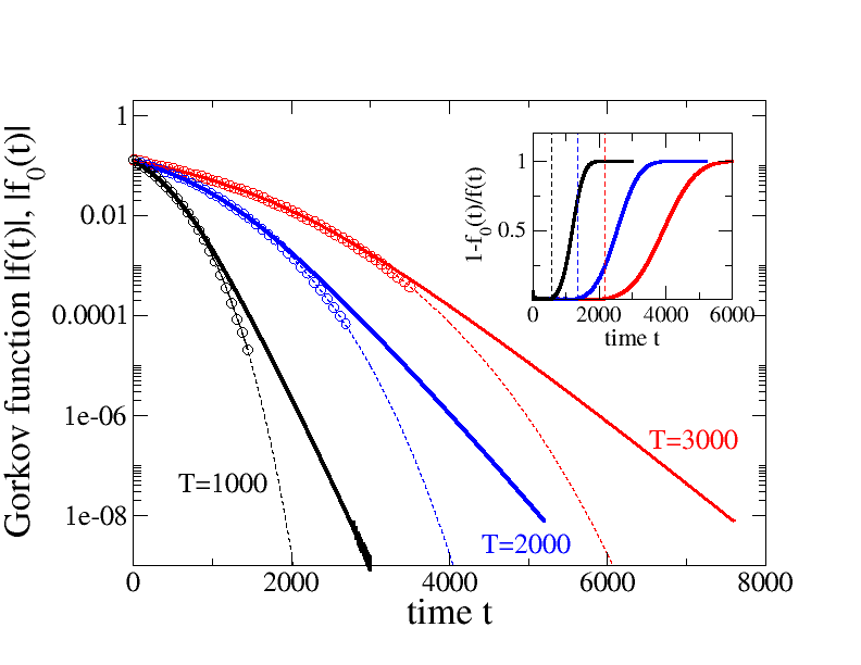
Figure 1: Time evolution of the Gorkov function $|f(t)|$ (solid lines) for different adiabatic time scales $T=1000$ (black), $T=2000$ (blue), and $T=3000$ (red). Circles correspond to the equilibrium values $|f_{0}(t)|$ obtained from the BCS equation for the interaction value $U(t)$ from Eq. (2) and the dashed lines are the corresponding parametrization from Eq. (26). The inset shows $1-f_{0}(t)/f(t)$ for the different adiabatic time scales in comparison with the time where the adiabaticity condition $d\Delta/dt<\Delta^{2}$ starts to get violated (dashed). Results are for a semielliptic DOS $\rho(\omega)=\frac{2}{\pi}\sqrt{B^{2}-\omega^{2}}$ with $B\equiv 1$ at density $n=0.875$ and an initial value of $U(t=0)=0.5$.

Figure 2 shows the time evolution of the total energy. For large enough adiabatic decay times $T$ the final energy approaches the equilibrium value for $U=0$, whereas this is overshot for small $T$. One can shed some light on this behavior by noticing that $U(t)$, as defined in Eq. (2), is invertible so that the time derivative in Eq. (23) can be transformed into a derivative in $U$, i.e.

$$\frac{dE}{dU}=-N\left(\frac{n^{2}}{4}+|f|^{2}\right)\,.$$ (28)

Then, it follows that the energy difference $\Delta E(t)$ between interacting system at time $t=0$ and the final system at time $t$ is given by

$$\Delta E(t)=-N\int_{U_{0}}^{U(t)}dU\left(\frac{n^{2}}{4}+|f|^{2}\right)=\int_{0}^{t}\frac{dE}{dt}dt$$ (29)

where in a complete adiabatic process the Gorkov function can be replaced by its equilibrium value $f_{0}$.

For small decay times $T$, the dynamic Gorkov function $f(t)$ overestimates the adiabatic equilibrium value already at an early stage of the time evolution leading therefore also to an overestimation of $\Delta E(t\to\infty)$. This difference between $f(t)$ and $f_{0}$ decreases with increasing $T$ and for $T\gtrsim 1000$ the difference between $E(t)$ and the energy of the non-interacting Fermi liquid cannot be resolved on the scale of the plot.

Figure 2: Time dependence of the energy per site for different adiabatic time scales. The horizontal grey is the equilibrium value for $U=0$. System and parameters are the same than in Fig. 1.

The energy dependence of the pseudospins $J_{k}^{x,y,z}$, Eqs. (18, 19, 20), for two times $t=300$ and $t=3000$ and interaction decay time $T=2000$ is shown in Fig. 3. In the BCS approximation these quantities are given by

$$J_{k}^{x} = -\frac{1}{2}\frac{|\Delta|\cos(\phi)}{\sqrt{|\Delta|^{2}+\xi_{k}^{2}}}$$ (30)

$$J_{k}^{y} = \frac{1}{2}\frac{|\Delta|\sin{\phi}}{\sqrt{|\Delta|^{2}+\xi_{k}^{2}}}$$ (31)

$$J_{k}^{z} = -\frac{1}{2}\frac{\xi_{k}}{\sqrt{\Delta^{2}+\xi_{k}^{2}}}$$ (32)

where $\phi$ was defined in Eq. (8).

Since we are in the adiabatic regime, the pseudospins at $t=300$ are fully compatible with the BCS result when evaluated with the gap $\Delta(t=300)$ and phase $\phi(t=300)$ at the same time. However, minute deviations of the individual phases $\phi_{k}=\arctan(J_{k}^{y}/J_{k}^{x})$ from the global phase $\Phi\approx 0.03$ are already apparent as shown in the inset to Fig. 3. The issue of a finite global phase will be discussed in Sec. II.3.

Figure 3: Dependence of $J_{k}^{\parallel}\equiv\sqrt{(J_{k}^{x})+(J_{k}^{y})}$ (a), the momentum dependent phase $\phi_{k}=\arctan(J_{k}^{y}/J_{k}^{x})$ [main panel (b) and inset] and $J_{k}^{z}$ (c) on $\varepsilon_{k}$ at times $t=300$ and $t=3000$ for an adiabatic decay time $T=2000$. The inset to (c) details the behavior of $J_{k}^{z}\approx 0$. Results are for a semielliptic DOS $\rho(\omega)=\frac{2}{\pi}\sqrt{B^{2}-\omega^{2}}$ with $B\equiv 1$ at density $n=0.875$ and an initial value of $U(t=0)=0.5$.

At large times $t=3000$ the gap tends to zero and $J_{k}^{z}$, Eq. (32) develops into a step function which in the present context of adiabatic behavior is nothing but the Fermi function at zero temperature. As can be seen from the inset to Fig. 3c, the energy at which $J_{k}^{z}$ equals zero changes with the time evolution of the system. In Sec. II.3 we will discuss how this shift is related to the change in the chemical potential. Far from the adiabatic limit, i.e. for $t\gg T$ (cf. Fig. 4), $J_{k}^{z}$ does not completely evolve into a step function but resembles a finite temperature Fermi function, though the functional form is different. This is of course related to the incomplete relaxation and the remaining excitations are responsible for the extended finite slope in $J_{k}^{z}$ around $\varepsilon_{k}=\mu$.

Figure 4: Same as panels (a,c) of Fig. 3 but for a small adiabatic decay time $T=200$ and $t=3000$.

Since the length of the pseudospins $|J_{k}^{x}|^{2}+|J_{k}^{y}|^{2}+|J_{k}^{z}|^{2}=1/4$ is conserved, a zero in $J_{k}^{z}$ implies maximum projection of $\vec{J}_{k}$ onto the other two components. Indeed, one finds that as a function of energy, the corresponding magnitude $J_{k}^{\parallel}=\sqrt{(J_{k}^{x})^{2}+(J_{k}^{y})^{2}}$ develops into a narrow spike at large times, cf. Fig. 3a. For $T=300$ this behavior can be understood as due to the residual gap, however, even for infinite times a hypothetical pseudospin at the position of the discontinuity in $J_{k}^{z}$ (i.e. at $J_{k}^{z}=0$) should remain out of equilibrium in such a way that $J_{k}^{\parallel}=1/2$.

Of course this depends on whether the state $\xi_{k}=0$ is an accessible state of the system or not. Thus, we first consider a finite system for which $\xi_{k}=0$ is not an accessible state in the sense that during the whole time evolution the chemical potential remains localized between two levels.

Then the density matrix for $t\to\infty$ takes the form

$$\underline{\underline{R}}_{\infty} = \frac{1}{2}(\underline{\underline{1}}+\underline{\underline{\tau_{z}}})\hskip 8.5359pt\mbox{for}\hskip 8.5359pt\xi_{k}<0$$

$$\underline{\underline{R}}_{\infty} = \frac{1}{2}(\underline{\underline{1}}-\underline{\underline{\tau_{z}}})\hskip 8.5359pt\mbox{for}\hskip 8.5359pt\xi_{k}>0$$ (33)

so that upon starting from a BCS superconductor and adiabatically switching off the interaction the system approaches a normal Fermi liquid with all states below (above) $\xi_{k}=0$ occupied (empty).

In the opposite limit, i.e. by first taking the large $N$ limit and then evaluating the dynamics for large times, the system always keeps memory of its initial superconducting state when approaching the Fermi liquid as there are always states sufficiently close to the sign change of $J_{k}^{z}$ which have a non-zero pseudospin component in the $xy$-plane. So in case of a decreasing interaction, no matter how slow and how small the final interaction is, the dynamics can be always inverted (see next subsection) at a given time and one returns to the superconducting state.

In the other case, i.e. if $\xi_{k}=0$ is an accessible state, then according to the above discussion, the density matrix for this level and in the limit $t\to\infty$ reads

$$\underline{\underline{R}}_{\infty}=\frac{1}{2}(\underline{\underline{1}}+\cos(\varphi)\underline{\underline{\tau_{x}}}-\sin(\varphi)\underline{\underline{\tau_{y}}})\hskip 8.5359pt\mbox{for}\hskip 8.5359pt\xi_{k}=0\,.$$ (34)

It can be shown Blaizot1986 that the density matrix describes a pure BCS state if and only if it is idempotent, i.e. $\underline{\underline{R}}^{2}=\underline{\underline{R}}$. One can check that this is the case for the above density matrix. Thus, the pseudospin at $\xi_{k}=0$ keeps track of the BCS origin of the state and $\varphi$ keeps memory of the original phase $\phi$ of the state. In Appendix B it is shown that such an initial state with only one transverse pseudospin component at $\xi_{k}=0$ evolves into a BCS state upon turning on the attractice interaction. However, the BCS recovery time scales with the system size so that in the thermodynamic limit the system stays inifinitely long in this unstable saddle point.

Notice that for a metal the density matrix at the chemical potential will normally be taken as $\underline{\underline{R}}=\frac{1}{2}\underline{\underline{1}}$ which is manifestly non idempotent. Indeed this density matrix does not correspond to a BCS state nor to a single Slater determinant (which requires $n_{k}^{2}=n_{k}$) but needs a mixed state to be represented.

Figure 5: Time dependence of the Gorkov function where the time evolution is reversed after $t_{0}=3000$ time steps with adiabatic time scales $T=2000$ (black) and $T=3000$ (red). Solid (dashed) lines correspond to the reversed time evolution with (without) inversion of the $J_{k}^{x,y}$ component. Interaction parameter $U(t=0)=0.5$; density $n=0.875$.

II.2 Time inversion of the dynamics

We now discuss the issue of inverting the dynamics after some given time $t_{0}$ where we will show that this requires the application of the equivalent of a $\pi$-pulse in an NMR Hahn echo experiment. hahn In fact, inspection of the equations of motion Eq. (21) reveals that $t\to-t$ implies $J_{k}^{x}\to-J_{k}^{x}$ or $J_{k}^{y}\to-J_{k}^{y}$ (and thus $f_{x}\to-f_{x}$ or $f_{y}\to-f_{y}$). The time inversion protocol is therefore specified as follows:

1. Evaluate the dynamics of the system with a decreasing interaction $U(t)=Ue^{-t/T}$ until a given time $t=t_{0}$.

2. At $t=t_{0}$ perform the rotation $J_{k}^{x}\to-J_{k}^{x}$ or $J_{k}^{y}\to-J_{k}^{y}$.

3. At $t=t_{0}$ transform to an increasing interaction $U(t)=U(t_{0})e^{(t-t_{0})/T}$ so that the total $U(t)$ is symmetric with respect to $t_{0}$ and the initial interaction is recovered at $t=2t_{0}$, i.e. $U(t=0)=U(2t_{0})=U$.

4. Evaluate the dynamics of the system which at $t=2t_{0}$ approaches the initial state.

Fig. 5 reveals that inversion of time with the concomitant inversion of one transverse pseudospin component, indeed, leads to symmetric behavior of the Gorkov function with respect to the inversion point at $t=t_{0}$. On the contrary, without inversion of $J_{k}^{x,y}$ the Gorkov function keeps decreasing after the time inversion thus showing an intrinsic inertia in some restricted time interval. Such inertial behavior can be understood by mapping the pseudospin dynamics to harmonic oscillators.OjedaCollado2021 In the present setting, for a negligible $\Delta$, the $J_{k}^{x}$ and $J_{k}^{y}$ components play the role of the canonical variables describing circles in phase space. The flip of $J_{k}^{y}$ corresponds to a sign change of the velocity at the inversion point. Without such inversion, the inertia tends to keep the original trajectory until the external drive takes over.

Notice that the above protocol keeps both phase and amplitude information, justifying our previous statement that the individual pseudospin phase at the chemical potential keeps information of the global phase of the parent superconductor.

Literally, the $\pi$-pulse NMR protocol to send $J_{k}^{y}\to-J_{k}^{y}$ would require a $\pi$-rotation along the $x$ direction which can be achieved here by a time-dependent $b_{k}^{x}$ due to a controllable Josephson coupling with another superconductor (or band). In addition, the field should be applied only to a small set of pseudospins close to the chemical potential in order to minimize the simultaneous introduction of charge fluctuations ($J_{k}^{z}\to-J_{k}^{z}$). In the present computation we introduced the $J_{k}^{y}$ flip “by hand” at the inversion time $t_{0}$, leaving for future work possible practical implementations by generalized external fields.

II.3 Global phase dynamics and chemical potential

The results of Sec. II.1, in particular energy $E(t)$ (Fig. 2) and $J_{k}^{z}(t)$ (Fig. 3) are evaluated using Eqs. (21, 22) with $\mu_{0}=const$. Indeed, $E(t)$ and $J_{k}^{z}(t)$ are gauge invariant quantities which do not depend on the phase $\phi$ of the order parameter. The phase $\phi$ of the order parameter is the conjugate variable to the charge density $n$ as can be seen from the Lagrangian Eq. (5). Since $E_{BCS}$ does not depend on $\phi$ the corresponding equation of motion $d/dt(\partial L/\partial\dot{\phi})=-N/2dn/dt=0$ implies particle number conservation during the dynamics.

We can make a gauge transformation that eliminates the time-derivative of $\phi$ in favor of a scalar potential that can be absorbed in the chemical potential so that in the new gauge $\phi$ is constant and $\mu$ becomes time-dependent. From the term with the time derivative of the phase in Eq. (5) it is clear that the gauge transformation is $\mu_{0}\to\mu(t)$ with

$$\mu(t)=\mu_{0}-1/2d\phi/dt\,.$$ (35)

This corresponds to a change of phase of the fermionic operator

$$c_{k,\sigma}\to c^{\prime}_{k,\sigma}e^{i\phi/2}$$ (36)

and at the same time the order parameter, transformed in the same way, becomes a real quantity.

Since the scalar potential appears as a pseudomagnetic field in the $z$ direction, the same result can be obtained by transforming the dynamics to the global Larmor frame of the precessing pseudospins

$$\frac{{d\bf J}_{k}}{dt}\longrightarrow\frac{{d\bf J^{\prime}}_{k}}{dt}+{\bf\Omega}\times{\bf J^{\prime}}_{k}\,.$$

with ${\bf\Omega}=(0,0,d\phi/dt)$ and ${\bf J^{\prime}}_{k}$ given by expressions (18)-(20) but in terms of the transformed fermion operators. This is in fact equivalent to applying the gauge transformation Eq. (36) which eliminates the phase of the Gorkov function $f$ and which therefore becomes purely real, i.e. $f^{\prime}_{y}=0$.

Figure 6: (a) Phase of the Gorkov function for the case $\mu=const.$ (black) and after transforming to the Larmor frame (red). (b) Time-dependent chemical potential from transforming to the Larmor frame (red), from the zeros of $J_{z}$ (black) and from the relation $\mu(t)=dE(n,t)/dn$ (blue). Density $n=0.875$, $U/t=1$, decay time $T=500$.

From a physical perspective this means that in order to follow an adiabatic dynamics, where at each instant of time one can obtain the solution from the BCS equation with interaction $U(t)$ and a real order parameter, also the chemical potential has to be adjusted according to Eq. (35).

Fig. 6a shows the time evolution of the phase for a given adiabatic decay time $T=500$ when the chemical potential in $E_{BCS}$ is fixed (black curve). Instead, when we transform to a time dependent chemical potential $\mu(t)$ according to Eq. (35) then the phase becomes time independent and equal to the initial value $\phi=0$ (red curve), i.e. the order parameter is a real quantity during the time evolution.

We can also define a time-dependent chemical potential from the sign change of $J_{k}^{z}$ motivated by the fact that this function develops into the Fermi step function for large times (cf. Fig. 3b). In the inset to Fig. 3b it becomes apparent that the energy $\varepsilon_{k}$, for which $J_{k}^{z}=0$, shifts during the dynamics of the system. In fact, in the Larmor frame the transformed $z$-component of the pseudomagnetic field reads $b_{z}^{\prime}=\varepsilon_{k}-\mu(t)-Un/2$ so that the solution for $b_{z}^{\prime}=0$ is given by $J_{k}^{{}^{\prime}x}=1/2$, $J_{k}^{{}^{\prime}y}=0$, $J_{k}^{{}^{\prime}z}=0$.

As can be seen from Fig. 6b, this leads to the same time dependent $\mu(t)$ as obtained by transforming to the Larmor frame. A further possibility is the computation of the time-dependent chemical potential from the relation

$$\mu(t)=\frac{1}{N}\frac{dE(n,t)}{dn}$$

where $E(n,t)$ denotes the total internal energy, not the grand canonical potential, $E_{BCS}(\mu,t)$. $E(n,t)$ is obtained from Eq. (6) setting $\mu_{0}=0$. Since $E(n,t)$ and $E(n+\delta n,t)$ are very close to the equilibrium value in an adiabatic evolution, it is clear that ${dE(n,t)}/{dn}$ should also be close to the equilibrium chemical potential and the chemical potential obtained with the other criteria as shown in Fig. 6b.

II.4 Restoring gauge invariance in BCS

While in the previous section we have considered the time evolution of a spatially homogeneous system, we will now consider the phase dynamics in case of a momentum dependent electromagnetic field. In particular, we will be interested in the question how, starting from an initially non-gauge invariant BCS state, gauge invariance is restored when we allow the phase to relax during the adiabatic time evolution.

II.4.1 Setting up the problem

In the presence of a static vector potential ${\bf A}({{\bf q}})$ the total current should respond according to

$$j_{\mu}({\bf q})=K_{\mu\nu}({\bf q})A_{\nu}({\bf q})$$ (37)

where in the long-wave length limit

$$K_{\mu\nu}({\bf q})=\left[\delta_{\mu\nu}-\frac{q_{\mu}q_{\nu}}{q^{2}}\right]K(q^{2})$$ (38)

as a consequence of gauge invariance and charge conservation.Schafroth

A superconductor and a conventional metal can be distinguished by different limiting behavior of the transverse current response to an applied static vector potentialschrieff ; scalapino93 ; and1 ; and2 ; gaugin $\lim_{{\bf q}\to 0}{\bf j}({\bf q})=\lim_{{\bf q}\to 0}D_{s}({\bf q}){\bf A}({\bf q})$. If the limit ${\bf q}\to 0$ is taken for a momentum ${\bf q}\perp{\bf A}$, then the superfluid stiffness $D_{s}$ is finite for a superconductor whereas it vanishes in the metal. However, for the BCS superconductor, defined from the variational wave-function Eq. (3) with a spatially uniform phase, one obtains the same result when the limit ${\bf q}\parallel{\bf A}$ is considered, whereas it should vanish in a gauge invariant approach [cf. Eq. (38)], as it does in the non-interacting metal.

Without loss of generality we fix ${\bf A}({\bf q})\equiv A_{x}({\bf q}){\bf e}_{x}$ and introduce the following definitions for the longitudinal and transverse responses

$$j_{x}(q_{x}\to 0,q_{y}=0) = D_{l}(q_{x})A_{x}(q_{x})$$ (39)

$$j_{x}(q_{x}=0,q_{y}\to 0) = D_{t}(q_{y})A_{x}(q_{y})$$ (40)

$$= D_{s}(1-\xi_{t}^{2}q_{y}^{2})A_{x}(q_{y})\,.$$

Here $D_{s}$ is the superfluid stiffness and we introduced $\xi_{t}$, the superconducting correlation length.

These investigations require the implementation of a momentum dependent vector potential so that the evaluation of time dependent quantities in terms of a density of states is not longer possible. Our model system is a square lattice with nearest-neighbor hopping and periodic boundary conditions for $A_{x}$.

For evaluating the transverse response we therefore consider the coupling

$$\hat{T}_{x}=-t\sum_{ix,iy,\sigma}\left[c^{\dagger}_{ix,iy,\sigma}c_{ix+1,iy,\sigma}e^{-iA_{x}(iy)}+h.c.\right]$$ (41)

with $A_{x}(iy)=A_{0}\cos(q_{y}i_{y})$ and we leave translational invariance along the $x$-direction.

The longitudinal coupling is given by

$$\hat{T}_{x}=-t\sum_{ix,iy,\sigma}\left[c^{\dagger}_{ix,iy,\sigma}c_{ix+1,iy,\sigma}e^{-iA_{x}(ix)}+h.c.\right]$$ (42)

with $A_{x}(ix)=A_{0}\cos(q_{x}i_{x})$ and translational invariance is kept along the $y$-direction. In both cases the total current $j_{x}=-\partial\hat{T}_{x}/\partial A_{x}$ can be decomposed into a para- and diamagnetic part $j_{x}=j_{para}+j_{dia}$, cf. Appendix A.

With these definitions the superconducting correlation length is,

$$\xi_{t}^{2}=\frac{8t^{4}}{D_{s}}\frac{1}{N}\sum_{k}\sin^{2}(k_{x})\sin^{2}(k_{y})\frac{1}{E_{k}^{3}}\left(1-\frac{\varepsilon_{k}^{2}}{E_{k}^{2}}\right)$$ (43)

as obtained from the current-current correlation function, cf. e.g. Ref. scalapino93, . As will be shown explicitly below, the longitudinal vector potential can be eliminated from the problem so that physical observables do not depend on it. Therefore, in a gauge invariant approach,

$$D_{l}(q_{x})=0\,.$$ (44)

Figure 7: Main panel: Static response to an external vector potential. Black: Transverse response to $A_{x}(q_{y})$; Blue: (Gauge invariant) Longitudinal response to $A_{x}(q_{x})$; Red: Longitudinal response in the BCS approximation. Dashed lines correspond to Eqs. (43, 46) with $\xi_{t}=1.88$, $\xi_{l}=1.96$. Inset: Spatial variation of the order parameter phase for the (gauge invariant) longitudinal response. Parameters: $U/t=0.5$, $n=0.875$, $72\times 72$ lattice.

As mentioned above, Eq. (44) is violated in the rigid-phase BCS approximation where

$$j^{BCS}_{x}(q_{x}\to 0,q_{y}=0)=D_{s}^{0}(1-\xi_{l}^{2}q_{x}^{2})A_{x}(q_{x})\,.$$ (45)

i.e. for $q_{x}\to 0$ it approaches the same limit than in the transverse case, however, the correlation length is different and given by

$$\xi_{l}^{2}=\frac{8t^{4}}{D_{s}}\frac{1}{N}\sum_{k}\sin^{4}(k_{x})\frac{1}{E_{k}^{3}}\left(1-\frac{\varepsilon_{k}^{2}}{E_{k}^{2}}\right)\,.$$ (46)

It has been shown by Anderson and1 ; and2 and Rickayzen rick59 that the longitudinal, in contrast to the transverse, response couples to collective phase modes of the order parameter and in this way gauge invariance can be restored.

In the normal metal the superfluid stiffness $D_{s}$ vanishes so that both, the longitudinal and transverse response Eqs. (39,40) vanish in this case. It is therefore interesting to study the time dependent approach of a BCS superconductor to the non-interacting limit and to follow the time evolution of the longitudinal and transverse response.

Figure 8: Finite size effects for the adiabatic transition of the Gorkov function with $U(t)=U_{0}e^{-t/T}$ and $T=500$. The dynamics for the infinite lattice blue dashed) has been computed with the 2-dim DOS. Parameters: $U_{0}/t=0.5$, $n=0.875$.

Figure 7 compares the transverse and longitudinal equilibrium response for a finite system and demonstrates the agreement with the expansion at small momenta given by Eqs. (43,46).

II.4.2 Irrelevance of a longitudinal vector potential

The problem of the superconductor coupled to a longitudinal vector potential can be mapped to a superconductor without such coupling. Thus, the longitudinal vector potential can be “gauged away” and is physically irrelevant. Within our definition of the coupling Eq. (42), the gauge transformation to new operators $c_{ix,iy,\sigma}^{\prime}$ reads,

$$c_{ix,iy,\sigma}^{\prime}=c_{ix,iy,\sigma}\exp\left[-i\sum_{i_{x}^{\prime}=0}^{i_{x}-1}A_{x}(i_{x}^{\prime})\right].$$

where $i_{x}=0,..,L-1$ and $A_{x}(L)=A_{x}(0)$. This relation implies that

$$c_{L,iy,\sigma}^{\prime}=c_{L,iy,\sigma}\exp\left[-i\sum_{i_{x}^{\prime}=0}^{L-1}A_{x}(i_{x}^{\prime})\right]=c^{\prime}_{0,iy,\sigma}.$$

which allows to close the boundary conditions without any effect of the longitudinal field. In terms of the new operators the kinetic energy reads like Eq. (42) but without any vector potential. Since for local observables the phase factors are irrelevant, it follows that any physical observable can not depend on the longitudinal field.

We can now use the inverse transformation to understand the equilibrium solution in the original variables. Once the vector potential has been eliminated, we can assume an equilibrium Gorkov function with spatially uniform phase $f^{\prime}={const.}$ Transforming back to the old operators one obtains a Gorkov function,

$$f(i_{x})=f^{\prime}\exp\left[2i\sum_{i_{x}^{\prime}=0}^{i_{x}-1}A_{x}(i_{x}^{\prime})\right]$$ (47)

so that gauge invariance completely determines the phase of the order parameter in the original variables. Since $A_{x}(i_{x}^{\prime})\propto\cos(q\,i_{x})$ for small $q$ we can use the continuum limit to show that the phase of the Gorkov function should behave as $\phi\propto\sin(q\,i_{x})/q$ (cf. inset to Fig. 7). Clearly, this is in contrast with the rigid-phase BCS approximation where $\phi\equiv 0$ yields the incorrect result $D_{l}(q_{x}\to 0,q_{y}=0)=D_{t}(q_{x}=0,q_{y}\to 0)$ which is equivalent to the (negative) kinetic energy along the direction of the applied vector potential.

Due to the above mapping, the adiabatic evolution of a system with a longitudinal vector potential is equivalent to the corresponding dynamics of a uniform system. The phase of the order parameter is related to the uniform case by Eq. (47), so the spatial modulation does not depend on time. It is therefore more interesting to study the time evolution when the initial state is prepared in the non-gauge invariant BCS state Eq. (3) with a uniform phase, and gauge invariance has to be restored during the time evolution towards the non-interacting system. In the transverse case a similar gauge transformation cannot be done as $\sum_{i_{x}^{\prime}=1}^{L}A_{x}(i_{y})\neq 0$. The adiabatic dynamics of these two cases is studied below.

II.4.3 Finite size effects

The necessity of considering finite lattices implies finite size effects in the time evolution which are shown in Fig. 8 for the dynamics of the Gorkov function $|f|$. At long times this function does not approach $|f|=0$ as expected for the infinite system but one observes oscillations around finite values due to incomplete dephasing. Therefore results below are only strictly valid for a limited time interval, nevertheless we can draw some conclusions about the general behavior at large times.

Figure 9: Time dependence of the longitudinal response when the initial state is computed in the BCS approximation. a) Dia- (red) and paramagnetic (black) currents for $q_{x}=2\pi/72$. b) Total response $D_{l}=(j_{para}+j_{dia})/A_{0}$ for for $q_{x}=2\pi/72$ (black) and $q_{x}=8\pi/72$ (red). Parameters: $U_{0}/t=0.5$, $n=0.875$. $72\times 72$ lattice.

II.4.4 Restoring gauge invariance with a longitudinal field

For an exponential decay of the interaction $U=U_{0}e^{-t/T}$ with $T=500$, Fig. 9 reports the longitudinal response when the initial state is prepared in the non-gauge invariant BCS state Eq. (3), i.e. the order parameter phase is set to $\phi=const.\equiv 0$. In the time evolution instead, we allow the phase to relax. Therefore, even in the presence of $A(i_{x})$, the initial paramagnetic current vanishes, $j_{para}(t=0)=0$, whereas the diamagnetic current corresponds to the kinetic energy $-\langle t_{x}\rangle$ of the initial BCS solution. For large times the latter approaches $-\langle t^{0}_{x}\rangle$ of the non-interacting system whereas the paramagnetic current undergoes decaying low frequency oscillations. The total response (cf. Fig. 9b) therefore decays from the initial $D_{l}(q_{x},t=0)=-\langle t_{x}\rangle(t=0)$ to $D_{l}(q_{x},t\to\infty)\approx 0$ thus restoring gauge invariance at large times.

Figure 10: Phase mode along a selected momentum cut in the Brillouin zone. The linear approximation at small momenta is $\omega_{q}=0.25q$ and fits to the observed phase excitations in the current shown in Fig. 9. Parameters: $U/t=0.5$, $n=0.875$.

The frequency of the initial oscillations in $j_{para}$ linearly increases with $q_{x}$ and can be attributed to phase modes. In Fig. 10 we show the dispersion of phase excitations across the Brillouin zone for the same parameters, as obtained from an RPA calculation on top of the initial BCS state, and it turns out that the oscillations appearing in Fig. 9 fit to the sound mode $\omega\approx 0.113q_{x}$ which is shown as the linear fit at small momenta in Fig. 10.

Figure 11: Time dependence of the transverse response. a) Dia- and paramagnetic currents for different momenta $q_{y}$. b) Total response $D_{t}(q_{y},t)=(j_{para}+j_{dia})/A_{0}$. The inset compares the time dependent correlation length (solid) with the linear response expression Eq. (43). Parameters: $U_{0}/t=0.5$, $n=0.875$. $72\times 72$ lattice.

II.4.5 Time-dependent transverse response

The transverse response is analyzed in Fig. 11. Because of London rigidity, the phase is constant in the presence of the transverse vector potential. We find that also in the non-equilibrium state the phase does not couple to the response, i.e. also for an applied vector potential $A_{x}(q_{y})$ the order parameter phase stays spatially homogeneous. Thus, the dynamics occurs purely on the BCS level and, as a consequence, the time-dependent response at zero transverse momentum $D_{s}^{0}(q_{y}=0)$ is simply given by the time-dependent kinetic energy $-\langle t_{x}\rangle$ along the direction of the applied vector potential. This is shown in Fig. 11a which reports the time evolution of the paramagnetic current for different momenta $q_{y}$ of the applied vector potential.

Since the relation between diamagnetic current and vector potential is local (i.e. ${\bf j}_{dia}(ix,iy)\propto{\bf A}(ix,iy)$ the diamagnetic contribution (black curve) is independent of momentum.

At $q_{y}=0$ the paramagnetic current vanishes whereas $j_{dia}/A_{0}$ evolves from the kinetic energy of the BCS superconductor to the kinetic energy of the non-interacting metal. For finite $q_{y}$ and in the long-time limit $-j_{para}$ approaches the diamagnetic current so that in this limit the total finite momentum response tends to zero, cf. panel (b). Thus, the transition from a superconducting to normal state via the adiabatic transition is completed when $D_{t}(q_{y})=0$ for the smallest momentum $q_{y}$ so that $\lim_{q_{y}\to 0}D_{t}(q_{y})=D_{s}^{0}=0$, i.e. zero superfluid stiffness. Note that in our case, due to finite size effects, $D_{t}(q_{y},t\to\infty)$ approaches a small finite value only.

In fact, the transition should be accompanied by a diverging correlation length which in a finite lattice is always limited by the system size, i.e. $\xi_{max}=1/q_{y}^{min}$. This is shown in the inset to panel (b) which compares $\xi$ with the corresponding linear response result Eq. (43). For our finite lattice $\xi$ tends to saturate at $\xi=72/(2\pi)\approx 12$ (solid line) whereas the thermodynamic result (dashed) shows the expected divergence.

III Discussion and Conclusions

In this paper we have performed a comprehensive analysis of the phase dynamics when a BCS superconductor evolves into a non-interacting Fermi liquid by means of an exponentially decaying pairing interaction $U(t)$ with time scale $T$. Adiabaticity is obeyed when at each instant of time the order parameter obeys the corresponding BCS equation for the instantaneous interaction parameter $U(t)$. We have shown that for times $t\lesssim T$ this condition is fulfilled, which agrees with the condition that in this regime the rate of change of the gap is smaller than the square of the gap. polkov11 Thus, in order to preserve adiabaticity the change in $U$ should be slower than the closing of the gap and a Fermi liquid with $\Delta=0$ can only be reached in the limit $T\to\infty$.

One can make the evolution slow enough so that at long times $t\gg T$, where the gap becomes negligibly small, the momentum distribution appears as a step within a given resolution. However, in the thermodynamic limit, memory of the superconducting origin of this “Fermi liquid” is still preserved in the orientation of Anderson pseudospins close to the Fermi level. This was demonstrated by showing that one can fully recover the original BCS state by inverting the dynamics at a very long time. In this context, we have discussed the analogy between the reversed dynamics and spin/photon echo experiments. In principle, the inversion of time evolution can be experimentally investigated in ultracold quantum gases where extensive control of interactions is possible. lv20

The memory of the superconducting state can be erased if one inverts the order of limits, i.e. by first considering $t\to\infty$ for a finite system then taking the thermodynamic limit. In this case one reaches a perfect metal at $T=0$ in which all levels are either empty or occupied, i.e. for each state the Anderson pseudospins are oriented along $\pm z$.

We also studied the evolution of the phase, which in our system is not constrained to be constant by particle hole-symmetry. The requirement, that at each instant of time the solution can be described by the BCS equation with a real valued order parameter requires the implementation of a time-dependent chemical potential $\mu(t)$. We have shown that formally $\mu(t)$ can be obtained from the time-derivative of the phase $\dot{\phi}$ since phase and charge are conjugate variables in the problem. The same $\mu(t)$ results from the sign change of the pseudospin variable $J_{k}^{z}$ which in the adiabatic limit evolves into the zero temperature Fermi distribution. Moreover, it turned out that the same time-dependent chemical potential obeys the thermodynamic relation $\mu(t)=\partial E/\partial n$.

Finally, we have explicitely shown how gauge invariance is restored when the BCS superconductor with broken $U(1)$ symmetry, evolves into the Fermi liquid. The longitudinal response to an applied vector potential is corrected by the coupling to phase fluctuations which guarantee the vanishing of the corresponding current at smallest momenta and large times. For the transverse coupling it turned out that the phase does not couple, so that the corresponding physics in the time dependent situation is the same than in the stationary case. It has has been reported yus06 that in a quench situation where the order parameter drops to zero the superfluid stiffness reduces to half of $-\langle t_{x}\rangle$, however, this result seems to be incompatible with the present findings. This may be due to the fact that the response in Ref. yus06, has only be considered for zero momentum, whereas, as detailed in Sec. II.4, the superfluid stiffness has to be formally evaluated from the proper zero momentum limit.

Appendix A Evaluation of the transverse and longitudinal response

A.1 Transverse response

For the considered coupling to a transverse vector potential in Eq. (41) one can perform a Fourier transformation along the $x$-direction to the resulting hamiltonian $H=\sum_{kx}H(k_{x})$ with

$$H(k_{x}) = -2t\sum_{iy}\left[\cos(k_{x}-A_{x}(i_{y}))c_{kx,\uparrow}^{\dagger}(i_{y})c_{kx,\uparrow}(i_{y})\right.$$ (48)

$$- \left.\cos(k_{x}+A_{x}(i_{y}))c_{-kx,\downarrow}(i_{y})c^{\dagger}_{-kx,\downarrow}(i_{y})\right]$$

$$- t\sum_{iy}\left[c^{\dagger}_{kx,\uparrow}(i_{y}+1)c_{kx,\uparrow}(i_{y})\right.$$

$$- \left.c_{-kx,\downarrow}(i_{y}+1)c^{\dagger}_{-kx,\downarrow}(i_{y})+h.c.\right]$$

$$+ \sum_{iy}\left[\Delta c^{\dagger}_{kx,\uparrow}(i_{y})c^{\dagger}_{-kx,\downarrow}(iy)+h.c.\right]$$

$$- |U(t)|\sum_{iy}\frac{n_{iy}}{2}\left[c^{\dagger}_{kx,\uparrow}(i_{y})c_{kx,\uparrow}(i_{y})\right.$$

$$- \left.c_{kx,\downarrow}(i_{y})c^{\dagger}_{kx,\downarrow}(i_{y})\right]$$

For each momentum $k_{x}$ the hamiltonian can be diagonalized by a Bogoljubov de-Gennes (BdG) transformation

$$c_{kx,\sigma}(iy)=\sum_{p}\left[u_{iy,kx}(p)\gamma_{p,\sigma}(k_{x})-\sigma v_{iy,kx}(p)^{*}\gamma_{p,-\sigma}^{\dagger}(k_{x})\right]$$ (49)

which for each momentum allows to construct the density matrix $\underline{\underline{R}}(k_{x})$. For a $N\times N$ lattice it has dimension $2N\times 2N$ and obeys the equation of motion Eq. (17).

In order to define dia- and paramagnetic currents we expand Eq. (48) in powers of the vector potential

$$H(k_{x}) = H(k_{x},A_{x}=0)$$

$$- \sum_{iy}\left[j^{x}_{para}(k_{x},i_{y})A_{x}(i_{y})+\frac{1}{2}j^{x}_{dia}(k_{x},i_{y})A^{2}_{x}(i_{y})\right]$$

with

$$j^{x}_{para}(k_{x},i_{y}) = 2t\sum_{\sigma}\sin(k_{x})\langle c^{\dagger}_{kx,\sigma}(i_{y})c_{kx,\sigma}(i_{y})\rangle$$

$$j^{x}_{dia}(k_{x},i_{y}) = -2t\sum_{\sigma}\cos(k_{x})\langle c^{\dagger}_{kx,\sigma}(i_{y})c_{kx,\sigma}(iy)\rangle$$

and the total current is given by

$$j_{tot}^{x}(k_{x},i_{y}) = -\frac{\delta H(k_{x})}{\delta{A_{x}(i_{y}}}$$

$$= j^{x}_{para}(k_{x},i_{y})+j^{x}_{dia}(k_{x},i_{y})A_{x}(i_{y})\,.$$

The currents shown in Fig. 11 correspond to the Fourier transformed quantities at $\pm q_{c}$ and thus are given by

$$j^{x}_{para}(q_{y}) = \frac{2t}{N}\sum_{\sigma,iy,kx}\sin(k_{x})\langle c^{\dagger}_{kx,\sigma}(i_{y})c_{kx,\sigma}(i_{y})\rangle e^{iq_{y}i_{y}}$$

$$j^{x}_{dia}(q_{y}) = -\frac{2tA_{0}}{N}\sum_{\sigma,iy,kx}\cos(k_{x})\langle c^{\dagger}_{kx,\sigma}(i_{y})c_{kx,\sigma}(i_{y})\rangle$$

A.2 Longitudinal response

For the longitudinal coupling Eq. (42) the Fourier transformation is performed along the $y$-direction and the resulting hamiltonian $H=\sum_{ky}H(k_{y})$ reads

$$H(k_{y}) = -t\sum_{ix}\left[e^{-iA_{x}(ix)}c_{ky,\uparrow}^{\dagger}(i_{x})c_{ky,\uparrow}(i_{x}+1)\right.$$ (51)

$$- \left.e^{iA_{x}(ix)}c_{-ky,\downarrow}(i_{x})c^{\dagger}_{ky,\downarrow}(i_{x}+1)+h.c.\right]$$

$$- 2t\sum_{ix}\cos(k_{y})\left[c^{\dagger}_{ky,\uparrow}(i_{x})c_{ky,\uparrow}(i_{x})\right.$$

$$- \left.c_{-ky,\downarrow}(ix)c^{\dagger}_{-ky,\downarrow}(ix)\right]$$

$$+ \sum_{iy}\left[\Delta(i_{x})c^{\dagger}_{ky,\uparrow}(i_{x})c^{\dagger}_{-ky,\downarrow}(ix)+h.c.\right]$$

$$- |U(t)|\sum_{ix}\frac{n_{ix}}{2}\left[c^{\dagger}_{ky,\uparrow}(i_{x})c_{ky,\uparrow}(i_{x})\right.$$

$$- \left.c_{ky,\downarrow}(ix)c^{\dagger}_{ky,\downarrow}(i_{x})\right]$$

which can be diagonalized by a similar BdG transformation than in the transverse case.

For the longitudinal case we obtain the dia- and paramgnetic response from

$$j^{x}_{dia}(q_{x}) = -\frac{tA_{0}}{N}\sum_{ky,ix,\sigma}\left(\langle c_{ky,\uparrow}^{\dagger}(ix)c_{ky,\uparrow}(ix+1)\rangle+h.c.\right)$$

$$j^{x}_{para}(q_{x}) = \frac{it}{N}\sum_{ky,ix,\sigma}\left(\langle c_{ky,\uparrow}^{\dagger}(ix)c_{ky,\uparrow}(ix+1)\rangle-h.c.\right)e^{iq_{x}i_{x}}\,.$$

Appendix B Dynamics for an increasing interaction

Figure 12: Time dependence of the Gorkov function with the initial density matrix given by Eq. (33),(34) and a time dependent interaction $U(t)=U_{0}(\exp(t/T)-1)$. Parameters: $\varphi=0$, $U_{0}=0.5$, $T=1000$.

Fig. 12 shows the time evolution of the Gorkov function $f(t)$ for an exponentially increasing interaction and an initial density matrix given by Eqs. (33,34). Note that this does not correspond to the inverse time evolution of the dynamics shown in Fig. 1 since in this case the state Eq. (33) would only be reached for $t\to\infty$. Since one has a single ’nucleation state’ for superconductivity at the chemical potential the time evolution of $f(t)$ is clearly dependent on the number of energy levels $N$ so that in the limit of $N\to\infty$ the onset of exponential growth of $f(t)$ would be shifted to $t\to\infty$, i.e. one would stay in the Fermi liquid state for all times.

References

- (1) M. Born and V. A. Fock, Z. Phys. A 51, 165180 (1928).
- (2) M. Gell-Mann and F. Low, Phys. Rev. 84, 350 (1951).
- (3) S. Giorgini, L. P. Pitaevskii, and S. Stringari, Rev. Mod. Phys. 80, 1215 (2008).
- (4) P. Törmä, Phys. Scr. 91, 043006 (2016).
- (5) A. Polkovnikov, Phys. Rev. B 72, 161201 (2005).
- (6) J. Dziarmaga, Phys. Rev. Lett. 95, 245701 (2005).
- (7) W. H. Zurek, U. Dorner, and P. Zoller, Phys. Rev. Lett. 95, 105701 (2005).
- (8) T. Papenkort, V. M. Axt, and T. Kuhn, Phys. Rev. B 76, 224522 (2007).
- (9) T. Papenkort, T. Kuhn, and V. M. Axt, Phys. Rev. B 78, 132505 (2008).
- (10) G. Mazza and M. Fabrizio, Phys. Rev. B 86, 184303 (2012).
- (11) H. Krull, D. Manske, G. S. Uhrig, and A. P. Schnyder, Phys. Rev. B 90, 014515 2014).
- (12) J. Bünemann and G. Seibold, Phys. Rev. B 96, 245139 (2017).
- (13) G. Mazza, Phys. Rev. B 96, 205110 (2017).
- (14) H. P. O. Collado, J. Lorenzana, G. Usaj, and C. A. Balseiro, Phys. Rev. B 98, 214519 (2018).
- (15) H. P. Ojeda Collado, G. Usaj, J. Lorenzana, and C. A. Balseiro, Phys. Rev. B 99, 174509 (2019).
- (16) H. P. Ojeda Collado, G. Usaj, J. Lorenzana, and C. A. Balseiro, Phys. Rev. B 101, 054502 (2020).
- (17) M. Udina, T. Cea, and L. Benfatto, Phys. Rev. B 100, 165131 (2019).
- (18) G. Seibold and J. Lorenzana, Phys. Rev. B 102, 2469 (2020).
- (19) P. W. Anderson, Phys. Rev. 112, 1900 (1958).
- (20) R. A. Barankov, L. S. Levitov, and B. Z. Spivak, Phys. Rev. Lett. 93, 160401 (2004).
- (21) E. A. Yuzbashyan, B. L. Altshuler, V. B. Kuznetsov, and V. Z. Enolskii, J. Phys. A: Math. Gen. 38, 7831 (2005).
- (22) R. A. Barankov and L. S. Levitov, Phys. Rev. Lett. 96, 230403 (2006).
- (23) E. A. Yuzbashyan, O. Tsyplyatyev, and B. Altshuler, Phys. Rev. Lett. 96, 097005 (2006).
- (24) E. A. Yuzbashyan and M. Dzero, Phys. Rev. Lett. 96, 230404 (2006).
- (25) E. L. Hahn, Phys. Rev. 80, 580 (1950).
- (26) J. Bardeen, L. N. Cooper, and J. R. Schrieffer, Phys. Rev. 108, 1175 (1957).
- (27) J. P. Blaizot and G. Ripka, Quantum Theory of Finite Systems (The MIT Press, Cambridge, Massachusetts, 1986), pp. 1–657.
- (28) P. W. Anderson, Phys. Rev. 110, 827 (1958).
- (29) N. N. Bogoliubov, V. V. Tolmachov, and D. V. Širkov, Fortschr. Phys. 6, 605–682 (1958); Y. Nambu, Phys. Rev. 117, 648–663 (1960).
- (30) J. A. Scaramazza, P. Smacchia, and E. A. Yuzbashyan, Phys. Rev. B 99, 054520 (2019).
- (31) H. P. Ojeda Collado, G. Usaj, C. A. Balseiro, D. H. Zanette, and J. Lorenzana, Emergent parametric resonances and time-crystal phases in driven BCS systems, arXiv:2107.09683.
- (32) A. Polkovnikov, K. Sengupta, A. Silva, and M. Vengalattore, Rev. Mod. Phys. 83, 863 (2011).
- (33) E. A. Yuzbashyan and M. Dzero, Phys. Rev. Lett. 96, 230404 (2004).
- (34) M. R. Schafroth, Helv. Phys. Acta 24, 645 (1951).
- (35) J. R. Schrieffer, Theory of Superconductivity, Westview Press (1964).
- (36) D. J. Scalapino, S. R. White, and S. Zhang, Phys. Rev. B 47, 7995 (1993).
- (37) G. Rickayzen, Phys. Rev. 115, 795 (1959).
- (38) C. Lv, R. Zhang, and Q. Zhou, Phys. Rev. Lett. 125, 253002 (2020).