Group-based Motion Prediction for Navigation in Crowded Environments

Abstract

We focus on the problem of planning the motion of a robot in a dynamic multiagent environment such as a pedestrian scene. Enabling the robot to navigate safely and in a socially compliant fashion in such scenes requires a representation that accounts for the unfolding multiagent dynamics. Existing approaches to this problem tend to employ microscopic models of motion prediction that reason about the individual behavior of other agents. While such models may achieve high tracking accuracy in trajectory prediction benchmarks, they often lack an understanding of the group structures unfolding in crowded scenes. Inspired by the Gestalt theory from psychology, we build a Model Predictive Control framework (G-MPC) that leverages group-based prediction for robot motion planning. We conduct an extensive simulation study involving a series of challenging navigation tasks in scenes extracted from two real-world pedestrian datasets. We illustrate that G-MPC enables a robot to achieve statistically significantly higher safety and lower number of group intrusions than a series of baselines featuring individual pedestrian motion prediction models. Finally, we show that G-MPC can handle noisy lidar-scan estimates without significant performance losses.

1 Introduction

Over the past three decades, there has been a vivid interest in the area of robot navigation in pedestrian environments [1, 2, 3, 4, 5]. Planning robot motion in such environments can be challenging due to the lack of rules regulating traffic, the close proximity of agents and the complex emerging multiagent interactions. Further, accounting for human safety and comfort as well as robot efficiency add to the complexity of the problem.

To address such specifications, a common [3, 4, 6, 7, 8] paradigm involves the integration of a behavior prediction model into a planning mechanism. Recent models tend to predict the individual interactions among agents to enable the robot to determine collision-free candidate paths [3, 4, 9]. While this paradigm is well-motivated, it tends to ignore the structure of interaction in such environments. Often, the motion of pedestrians is coupled as a result of social grouping. Further, the motion of multiple agents can often be effectively grouped as a result of similarity in motion characteristics. Lacking a mechanism for understanding the emergence of this structure, the robot motion generation mechanism may yield unsafe or uncomfortable paths for human bystanders, often violating the space of social groups.

Motivated by such observations, we draw inspiration from human navigation to propose the use of group-based prediction for planning in crowd navigation domains. We argue that humans do not employ detailed individual trajectory prediction mechanisms. In fact, our motion prediction capabilities are short-term and do not scale with the number of agents. We do however employ effective grouping techniques that enable us to discover safe and efficient paths among motions of crowd networks. This anecdotal observation is aligned with gestalt theory from psychology [10] which suggests that organisms tend to perceive and process formations of entities, rather than individual components. Such techniques have recently led to advances in computer vision [11] and computational photography [12]. Similarly, we envision that a robot could reason the formation of effective groups in a crowded environment and react to their motion as an effective way to navigate safely.

In this paper, we propose a group-based representation coupled with a prediction model based on the group-space approximation model of Wang and Steinfeld [13]. This model groups a crowd into sets of agents with similar motion characteristics and draws geometric enclosures around them, given observation of their states. The prediction module then predicts future states of these enclosures. We conduct an extensive empirical evaluation over 5 different human datasets [14, 15], each with a flow following and a crossing scenario. We further conduct a same set of evaluations with agents powered by ORCA [16] that share the start and end locations in the datasets. Last but not least, we conducted evaluation given inputs in the form of simulated laser scans, from which pedestrians are only partially observable or even completely occluded. We compare the performance of our group-based formulation against three individual reasoning baselines: a) a reactive baseline with no prediction; b) a constant velocity prediction baseline; c) one based on individual S-GAN trajectory predictions [17]. We present statistically significant evidence suggesting that agents powered by our formulation produce safer and more socially compliant behavior and are potentially able to handle imperfect state estimates.

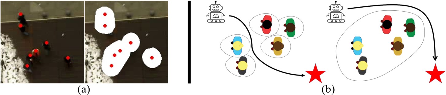
Figure 1: Based on a representation of social grouping [13], we build a group behavior prediction model to empower a robot to perform safe and socially compliant navigation in crowded spaces. (a) Example of our representation overlayed on top of a scene from a real-world dataset [14]. (b) A model predictive controller equipped with our prediction model is able to navigate around the group socially (right) as opposed to the baseline that cuts through the group (left).

2 Related Work

Over the recent years, a considerable amount of research has been placed to the problem of robot navigation in crowded pedestrian environments [3, 4, 8, 18, 19, 20, 21, 22, 23]. Such environments often comprise groups of pedestrians, navigating as coherent entities. Šochman and Hogg [24] suggests that $50$-$70\%$ of pedestrians walk in groups. Many works exist in group detection. One popular area in such domain is static group detection, often leveraging F-formation theories [25]. However, dynamic groups often dominate pedestrian-rich environments and exhibit different spatial behavior [26]. Among dynamic group detection, one common approach is to treat grouping as a probabilistic process where groups are a reflection of close probabilistic association of pedestrian trajectories [27, 28, 29, 30, 31]. Others use graph models to build inter-pedestrian relationships with strong graphical connections indicating groups [32, 33]. The social force model [34] also inspires Mazzon et al. [35], Šochman and Hogg [24] to develop features that indicate groups. Clustering is another common group of technique to group pedestrians with similar features into groups [36, 37, 38, 39]. For our formulation, it is sufficient to employ a simple clustering-based grouping method proposed by Chatterjee and Steinfeld [39]. Other grouping methods will simply result in different group membership assignments.

Applications on groups often focus on a specific behavior aspect. For example, one focus in this area is how a robot should behave as part of the group formation [40]. On dyad groups involving a single human and a robot, some researchers examined socially appropriate following behavior [41, 42, 43, 44] and guiding behavior [45, 46, 47]. In works that do not include robots as part of pedestrian groups, some research teams studied how a robot should guide a group of pedestrians [48, 49, 50]. From navigation perspective, Yang and Peters [26] leverage groups as obstacles, but their group space only involves occasional O-space modeling from F-formation theories. Without the engineered occurrence of O-space, their representation reduces to one of our baselines. Katyal et al. [51] introduce an additional cost term that leverages robot’s distance to the closest group in a reinforcement learning framework. They model groups using convex hulls directly generated from pedestrian coordinates instead of taking personal spaces into consideration. In our work, we additionally explore the capabilities of groups in handling imperfect sensor inputs. While our focus is on analysing the benefits of groups, our group based formulation can be easily incorporated into the work of Katyal et al. [51]’s framework.

3 Problem Statement

Consider a robot navigating in a workspace $\mathcal{W}\subseteq\mathbb{R}^{2}$ amongst $n$ other dynamic agents. Denote by $s\in\mathcal{W}$ the state of the robot and by $s^{i}\in\mathcal{W}$ the state of agent $i\in\mathcal{N}=\{1,\dots,n\}$. The robot is navigating from a state $s_{0}$ towards a destination $s_{T}$ by executing a policy $\pi:\mathcal{W}^{n+1}\times\mathcal{U}\to\mathcal{U}$ that maps the assumed fully observable world state $\boldsymbol{S}=s\cup_{i=1:n}s^{i}$ to a control action $u\in\mathcal{U}$, drawn from a space of controls $\mathcal{U}\subseteq\mathbb{R}^{2}$. We assume that the robot is not aware of agents’ destinations $s^{i}_{T}$ or policies $\pi_{i}:\mathcal{W}^{n+1}\times\mathcal{U}^{i}\to\mathcal{U}^{i}$, $i\in\mathcal{N}$. In this paper, our goal is to design a policy $\pi$ that enables the robot to navigate from $s_{0}$ to $s_{T}$ safely in a socially compliant fashion.

4 Group-based Prediction

We introduce a group representation building on prior work [13] and a model for group-based prediction that is amenable for use in decentralized multiagent navigation.

4.1 Group Representation

Define as $\theta^{i}\in[0,2\pi)$ the orientation of agent $i\in\mathcal{N}$ which is assumed to be aligned with the direction of its velocity $u^{i}$, extracted via finite differencing of its position over a timestep $dt$ and denote by $v^{i}=||u^{i}||\in\mathbb{R}^{+}$ its speed. We define an augmented state for agent $i$ as $q^{i}=(s^{i},\theta^{i},v^{i})$.

We treat a social group as a set of agents who are in close proximity and share similar motion characteristics. Assume that a set of $J$ groups, $\mathcal{J}=\{1,\dots,J\}$ navigate in a scene. Define by $g^{i}\in\mathcal{J}$ a label indicating the group membership of agent $i$. We then define a group $j\in\mathcal{J}$ as a set $G^{j}=\{i\in\mathcal{N}\mid g^{i}=j\}$ and collect the set of all groups in a scene into a set $\boldsymbol{G}=\{G^{j}\mid j\in\mathcal{J}\}$.

Extracting Group Membership. We define the combined augmented state of all agents as $\boldsymbol{q}=\cup_{i=1:n}q^{i}$. To obtain group memberships for a set of agents $\mathcal{N}$, we apply the Density-Based Spatial Clustering of Applications with Noise algorithm (DBSCAN) [52] on agent states:

$$\boldsymbol{G}\longleftarrow\texttt{DBSCAN}(\boldsymbol{q}\mid\epsilon_{s},\epsilon_{\theta},\epsilon_{v})$$ (1)

Where $\epsilon_{s},\epsilon_{\theta},\epsilon_{v}$ are respectively threshold values on agent distances, orientation and speeds.

Extracting the Social Group Space. For each group $G^{j}$, $j\in\mathcal{J}$, we define a social group space as a geometric enclosure $\mathcal{G}^{j}$ around agents of the group. For each agent $i\in G^{j}$, we define a personal space $\mathcal{P}^{i}$ as a two-dimensional asymmetric Gaussian based on the model introduced by Kirby [53]. Refer to Appendix A for detailed descriptions.

Given the personal spaces $\mathcal{P}^{i}$, $i\in G^{j}$, of all agents in a group $j$, we extract the social group space of the whole group as a convex hull:

$$\mathcal{G}^{j}=\mbox{Convexhull}(\{\mathcal{P}^{i}\mid i\in G^{j}\})\mbox{.}$$ (2)

The shape described by $\mathcal{G}^{j}$ represents an obstacle space representation of a group containing agents in close proximity with similar motion characteristics. For convenience, let us collect the spaces of all groups in a scene into a set $\boldsymbol{\mathcal{G}}=\{\mathcal{G}^{j}\mid j\in\mathcal{J}\}$.

4.2 Group Space Prediction Oracle

Based on the group-space representation of Sec. 4.1, we describe a prediction oracle that outputs an estimate of the future spaces occupied by a set of groups $\boldsymbol{\mathcal{G}}_{t:t_{f}}$ up to a time $t_{f}=t+f$, where $f$ is a future horizon given a past sequence of group spaces $\boldsymbol{\mathcal{G}}_{t_{h}:t}$ from time $t_{h}=t-h$ where $h$ is a window of past observations:

$$\boldsymbol{\mathcal{G}}_{t:t_{f}}\leftarrow\mathcal{O}(\boldsymbol{\mathcal{G}}_{t_{h}:t})=\cup_{j=1:J}\mathcal{O}_{j}(\mathcal{G}^{j}_{t_{h}:t})\mbox{,}$$ (3)

where $\mathcal{O}_{j}$ is a model generating a group space prediction for group $G^{j}$. Refer to Appendix B for detailed description of partial input handling.

We implement the oracle $\mathcal{O}_{j}$ of eq. (3) using a simple encoder-decoder network. The encoder follows the 3D convolutional architecture in [54] whereas the decoder mirrors the model layout of the encoder. The encoder-decoder network takes as input a sequence $\mathcal{G}_{t_{h}:t}$ and outputs a sequence $\mathcal{G}_{t+1:t_{f}}$ which we pass through a sigmoid layer. We supervise the encoder-decoder network’s output using the binary cross entropy loss.

We verified the effectiveness of our encoder-decoder network on the 5 scenes of our experiments by conducting a cross-validation comparison against a baseline. The baseline predicts the future shapes by linearly translating the last social group shape using its geometric center velocity. We use Intersection over Union (IoU) as our metric. Between the ground truths and the predictions, this metric divides the number of overlapped pixels by the number of pixels occupied by either one of them. As shown in Table 1, our encoder-decoder network outperforms the baseline.

Table 1: Prediction Model Performance

	Metric	ETH	HOTEL	ZARA1	ZARA2	UNIV
Baseline	mIoU (%)	83.52	90.37	88.04	89.30	85.32
	fIoU (%)	76.32	85.38	82.14	83.88	77.24
Encoder-decoder Network	mIoU (%)	86.66	92.10	89.97	90.94	87.52
	fIoU (%)	78.64	86.83	83.77	85.09	78.55

5 Model Predictive Control with Group-based Prediction

We describe G-MPC, a model predictive control (MPC) framework for navigation in multiagent environments that leverages the group-based prediction oracle of Sec. 4.

We describe our group-prediction informed MPC, or G-MPC. At planning time $t$, given a (possibly partial) augmented world state history $\boldsymbol{Q}_{t_{\hat{h}}:t}$, we first extract a sequence of group spaces $\boldsymbol{\mathcal{G}}_{t_{h}:t}$ based on the method of Sec. 4.1. Given these, the robot computes an optimal control trajectory $\boldsymbol{u}^{*}=u^{*}_{1:K}$ of length $K$ by solving the following optimization problem:

$$\left(\boldsymbol{s}^{*},\boldsymbol{u}^{*}\right)= \arg\min_{u_{1:K}}\sum_{k=1:}^{K}\gamma^{k}J(s_{k+1},\boldsymbol{\mathcal{G}}_{k+1},s_{T})$$ (4)

$$s.t.\> \boldsymbol{\mathcal{G}}_{2-h:1}\leftarrow\boldsymbol{\mathcal{G}}_{t_{h}:t}$$ (5)

$$s_{1}\leftarrow s_{t}$$ (6)

$$\boldsymbol{\mathcal{G}}_{k+1:k_{f}}=\mathcal{O}(\boldsymbol{\mathcal{G}}_{k_{h}:k})$$ (7)

$$u_{k}\in\mathcal{U}$$ (8)

$$s_{k+1}=s_{k}+u_{k}\cdot dt\mbox{,}$$ (9)

where $\gamma$ is the discount factor and $J$ represents a cost function, eq. (5) initializes the group space history ($k=2-h$ is the timestep displaced a horizon $h$ in the past from the first MPC-internal timestep $k=1$), eq. (6) initializes the robot state to the current robot state $s_{t}$, eq. (7) is an update rule recursively generating a predicted future group sequence up to timestep $k_{f}=k+f$ given history from time $k_{h}=k-h$ up to time $k$, $\mathcal{O}$ represents a group-space prediction oracle based on Sec. 4, and eq. (9) is the robot state transition assuming a fixed time parametrization of step size $dt$.

We employ a weighted sum of costs $J_{g}$ and $J_{d}$, penalizing respectively distance to the robot’s goal and proximity to groups:

$$J(s_{k},\boldsymbol{\mathcal{G}}_{k},s_{T})=\lambda J_{g}(s_{k},s_{T})+(1-\lambda)J_{d}(s_{k},\boldsymbol{\mathcal{G}}_{k})\mbox{,}$$ (10)

where $\lambda$ is a weight representing the balance between the two costs and

$$J_{g}(s_{k})=\begin{cases}0,&\mbox{if}\>s_{k}\in\boldsymbol{\mathcal{G}}_{k}\\ ||s_{k-1}-s_{T}||,&\mbox{else,}\end{cases}$$ (11)

penalizes a rollout according to the distance of the last collision-free waypoint to the robot’s goal. Further, we define $J_{d}$ as:

$$J_{d}(s_{k},\boldsymbol{\mathcal{G}}_{k})=\exp(-\mathcal{D}\left(s_{k+1},\boldsymbol{\mathcal{G}}_{k})\right)\mbox{,}$$ (12)

where

$$\mathcal{D}(s_{k},\boldsymbol{\mathcal{G}}_{k})=\begin{cases}\min_{j\in\mathcal{J}}D\left(s_{k}-\mathcal{G}_{k}^{j}\right),\>&\mbox{if}\>s_{k}\notin\mathcal{G}^{j}_{k}\\ -\min_{j\in\mathcal{J}}D\left(s_{k}-\mathcal{G}_{k}^{j}\right),\>&\mbox{else}\mbox{,}\end{cases}$$ (13)

where $D(s_{k}-\mathcal{G}_{k}^{j})$ returns the minimum distance between the robot state and the space occupied by group $j$ at time $k$. Using $D$, function $\mathcal{D}$ computes the minimum distance to any group for a given time. In most cases, the robot lies outside of groups, i.e., $s_{k}\notin\mathcal{G}^{j}_{k}$ –therefore, the cost $J_{d}$ tries to maximize the distance $\mathcal{D}$. Sometimes, the robot might end up entering the group space $\boldsymbol{\mathcal{G}}$ –in those cases, $J_{d}$ tries to minimize $\mathcal{D}$, to steer the robot towards the direction of quickest escape from the group. In case that the robot is inside a group to begin with, we shrink the group sizes in Sec. 4.1 until the robot is outside the groups again.

To solve eq. (4), we search over a finite set $\boldsymbol{\mathcal{U}}$ of control trajectories of horizon $K$. With the assumption that the robot is holonomic and is not under any kinematic constraints, we use a set of $R$ control rollouts $\boldsymbol{\mathcal{U}}=\{\boldsymbol{u}^{1},...,\boldsymbol{u}^{R}\}$ with three levels of tangential speeds and a set of turning speed, i.e.,

$$u_{1:K}^{r}=(v\cos\psi,v\sin\psi,\omega),\>\psi=\frac{2\pi r}{R},v\in\left\{\frac{1}{3}v_{max},\frac{2}{3}v_{max},v_{max}\right\},\omega\in\left\{0,\pm\frac{\pi}{2}\right\}$$ (14)

To ensure compatibility between our group-based prediction model and our MPC formulation, we set the control rollout time horizon to be the prediction model’s prediction horizon, or $K=f$.

6 Evaluation

We evaluate our framework through a simulation study in which the robot performs a navigation task (a transition between two points) within a crowds of dynamic agents in a set of scenes.

6.1 Experimental Setup

We consider a set of realistic pedestrian scenes, drawn from the ETH [14] (ETH and HOTEL scenes) and UCY [15] (ZARA1, ZARA2 and UNIVERSITY scenes) datasets, which often serve as benchmarking testbeds in the motion prediction and social navigation literature [17, 55, 56, 57, 58]. In each scene, we define two navigation tasks (see Fig. 2): Flow: in which the robot navigates along the crowd flow and Cross in which the robot intersects vertically with the traffic flow. For each task, we generate a set of trials by segmenting the scene recording into blocks involving challenging interactions. We define a challenging interaction to be a segment involving at least $5$ pedestrians inside the test region drawn in black in Fig. 2. This process provided us with a distribution of trials as shown in table Table 2. Across all trials, we keep the robot’s maximum speed at $1.75m/s$.

Table 2: Number of trials per task and scene.

Task	ETH	HOTEL	ZARA1	ZARA2	UNIV
Flow	58	43	25	127	106
Cross	58	44	28	129	114

We consider two experimental conditions: an Offline and an Online one. In the Offline one, the robot navigates among a crowd moving according to a recording of a human crowd. Under this condition, pedestrians act as dynamic obstacles that do not react to the robot, a situation which could arise in cases where robots are of shorter size and could thus be easily missed by navigating pedestrians. In the Online one, the robot navigates among a crowd moving by running ORCA [16], a policy that is frequently used as a simulation engine for benchmarking in the social navigation literature [8, 57, 59].

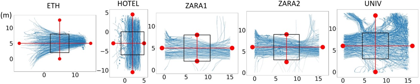
Figure 2: Trajectories of all pedestrians in the datasets. The red dots represent the task start and end locations. The red lines represent the task paths. The black box represents the test region to check for non-trivial tasks.

To investigate the value of G-MPC, we develop three variants of it. group-pred is a G-MPC in which the encoder-decoder network has a history $h=8$ and a horizon $f=8$. group-nopred is a variant that features no prediction at all –it just reacts to observed groups at every timesteps and it is equivalent to the framework of Yang and Peters [26]. Finally, laser-group-pred is identical to group-pred but instead of using ground-truth pose information, it takes as input noisy lidar scan readings. We simulate this by modeling pedestrians as $1m$-diameter circles and lidar scans as rays projecting from the robot. We refer to the spec sheet of a SICK LMS511 2D lidar for simulation parameters. We further inject noise into the readings according to the spec sheet. Under this simulation, pedestrians may only be partially observable or even completely occluded from the robot.

We compare the performance of these policies against a set of MPC variants using mechanisms for individual motion prediction. ped-nopred is a vanilla MPC that reacts to the current states of other agents without making predictions about their future states. ped-linear is a vanilla MPC that estimates future states of agents by propagating agents’ current velocities forward. This baseline is motivated by recent work showing that constant-velocity models yield competitive performance in pedestrian motion prediction tasks [60]. Finally, ped-sgan is an MPC that uses S-GAN [17] to extract a sequence of future state predictions for agents based on inputs of their past states. We selected S-GAN because it is a recent highly performing model. To ensure a fair comparison, all the MPC policy variants are integrated with the same MPC controller evaluated at $dt=0.1$.

We measure the performance of the policies with respect to four different metrics: a) Success rate, defined as the ratio of successful trials over total number of trials; b) Comfort, defined as the ratio of trials in which the robot does not enter any social group space over the total number of trials; c) Minimum distance to pedestrians, defined as the smallest distance between the robot and any agent per trial; d) Path length, defined as the total distance traversed by the robot in a trial.

To track the performance of G-MPC, we design hypotheses targeting aspects of safety and group space violation which we investigate under both experimental conditions, i.e., offline and online:

H1: To explore the benefits of group based representations alone, we hypothesize that group-nopred is safer than ped-nopred while achieving similar success rates but worse efficiency.

H2: To explore the full benefit of group based formulation, we hypothesize that group-pred is safer than ped-linear and ped-sgan while achieving similar success rates but worse efficiency.

H3: To explore how our formulation handles imperfect inputs, we hypothesize that laser-group-pred achieves similar safety to group-pred while achieving similar success rate and efficiency.

H4: To check that our formulation is socially compliant, we hypothesize that group-nopred, group-pred and laser-group-pred violate agents’ group space less often than the baselines.

6.2 Results

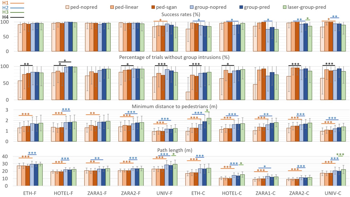
Figure 3: Performance per scene under the Offline condition. Horizontal lines indicate statistically significant results corresponding to different to hypotheses.

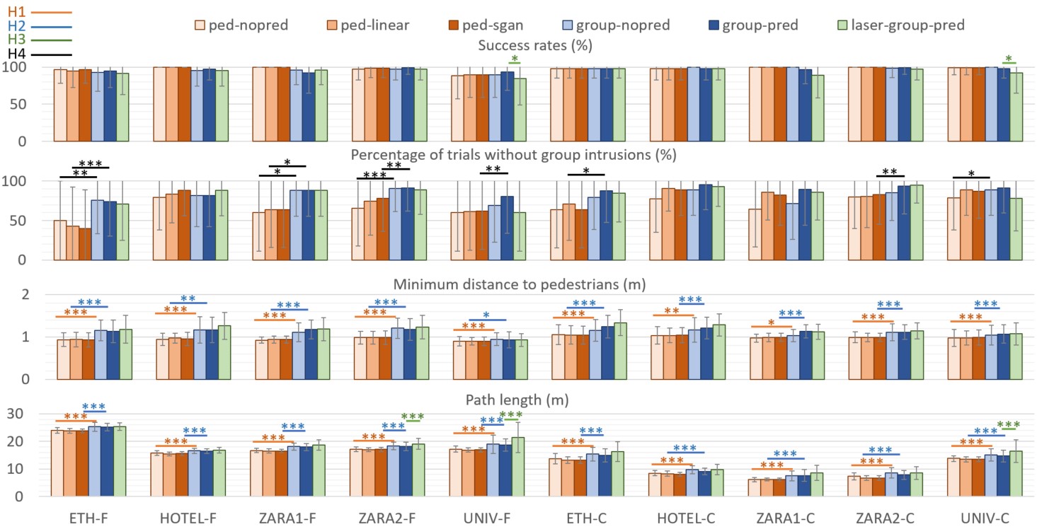
Figure 4: Performance per scene under the Online condition (simulated pedestrians powered by ORCA [16]). Horizontal lines indicate statistically significant results corresponding to different to hypotheses.

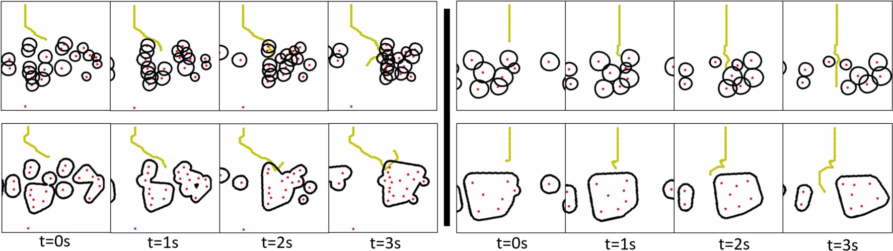
Figure 5: Qualitative performance difference between approaches leveraging pedestrian-based (top) and group-based (bottom) representations. Left: non-reactive agents. Right: reactive agents. In all cases, the robot starts from the top and attempts to navigate downward. The green line shows the robot’s traversed trajectory.

Quantitative Analysis. Fig. 3 and Fig. 4 contain bar charts representing the performance of G-MPC compared with its baselines under Offline and Online settings respectively. Bars indicate means, errorbars indicate standard deviations, “F” and “C” are flow and cross scenarios respectively, and the number of asterisks indicates increasing significance levels: $\alpha=0.05,0.01,0.001$ according to two-sided Mann-Whitney U-tests.

H1: We can see from both Fig. 3 and Fig. 4 that G-MPC achieves statistically significantly larger minimum distances to pedestrians across all scenarios, often with $p<0.001$. This illustrates that the group representation is in itself capable of upgrading a simple MPC with no prediction. As expected, we observe that the price G-MPC pays for that is a larger average path length. We also see that success rates are comparable. Overall, we conclude that H1 holds.

H2: When future state predictions are considered, G-MPC obtains statistically significant results in most scenes supporting its attributes of being safer at the cost of worse efficiency. Thus H2 is partially confirmed. In offline scenarios, G-MPC has lower success rates in crossing scenarios. Upon closer inspection, most failure cases are due to timeouts from G-MPC’s conservative behavior. However, in online scenarios where pedestrians react to the robot, G-MPC achieves high success rates. In real-world situations, to cross dense traffic, the robot needs to plan its actions with expectations of reactive pedestrians. Otherwise, the robot will most probably run into the freezing robot problem [4].

H3: Group-based representations have the potential to robustly account for imperfect state-estimates. Overall, we observe that with simulated imperfect states, G-MPC does not perform statistically significantly worse in terms of safety, but in dense crowds of the UNIV scenes it has worse efficiency and worse success rates in online cases. This shows that H3 holds in terms of safety and, in moderately dense human crowds, holds in terms of efficiency. Future work on better group representation is needed to achieve better efficiency in high-density human crowds given imperfect states.

H4: From Fig. 3 and Fig. 4, we can see that G-MPC often has fewer group-space intrusions than its baselines. While this relationship is not always statistically significant, we do see a general trend of the group-based approaches to respect group spaces more often than individual ones. Thus, we conclude that H4 is partially confirmed.

We additionally observe a general trend that group-pred is better than group-nopred in terms of higher success rates, lower chances of group intrusions, longer minimum distances to pedestrians and shorter path lengths. This shows that our group prediction model offers benefits to the robot’s navigation. However, in a few scenarios group-nopred performs better. We largely attribute this to the finite inaccuracies of future group predictions and the freezing robot problem that accompanies the robot’s more conservative behavior in group-pred than in group-nopred.

Qualitative Analysis. Qualitatively, it is a more common occurrence for regular MPC to perform aggressive and socially inappropriate maneuvers than G-MPC. As shown in the two examples in Fig. 5 executed by ped-sgan and group-pred agents, we can see that in offline conditions, the MPC agent aggressively cuts in front of the two pedestrians to the left before proceeding headlong into the cluster of pedestrians, only managing to avoid the deadlock by escaping through the narrow gap that opens up. While for G-MPC, it tracks the movements of the two pedestrian groups coming from the left. When the two pedestrian groups merge, the agent turns around and reevaluates its approach to cross. In the online condition, we observe that the MPC agent cuts through a pedestrian group to reach the other side, forcing a member of the group to stop and yield as indicated by the pedestrian’s shrinking personal space, which is proportional to its speed. In the same situation, the G-MPC agent chooses to circumvent behind the social group.

7 Conclusion

We introduced a methodology for generating group-based representations and predicting their future states. Through an extensive evaluation over the flow and crossing scenarios drawn from 10 different real-world scenes from 2 different human datasets with both reactive and non-reactive agents, we demonstrate the value of group-based prediction in enabling safe and socially compliant navigation. Through experimentation with simulated laser scans, our model displays promising potential to process noisy sensor inputs without much performance downgrade.

Several improvements to our framework are possible. For example, we could incorporate state-of-the-art oracles in the form of advanced video prediction models [61] or incorporate inter-group interaction modeling. Additional considerations such as the set of rollouts or the cost functions could possibly increase performance. We could also integrate our prediction model into alternative control frameworks such as reinforcement learning policies.

Finally, we plan on validating our findings on a real-world robot to fully test the capability of G-MPC to handle noisy sensor inputs. We also plan to investigate ways to improve computation time to enhance our approach’s real-world applicability. These include simplifying group representation geometry and predicting future group states in metric space instead of in image space.

Appendix

A Personal Space Definition

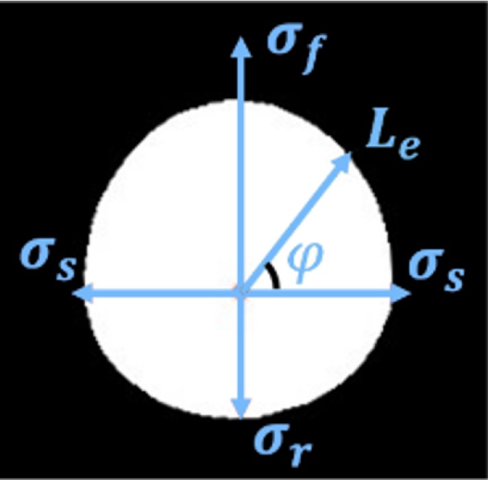
Figure 6: A sample personal space

An example of the personal space is shown in Fig. 6. Each personal space is first constructed by identifying the variances along the four principle axes to the agent’s front, sides and rear, defined respectively as:

$$\begin{split}\sigma_{f}^{i}&=\max(2v^{i},0.5),\\ \sigma_{s}^{i}&=2\sigma_{f}^{i}/3\\ \sigma_{r}^{i}&=\sigma_{f}^{i}/2\\ \end{split}\mbox{.}$$ (15)

Based on the four principle axis, the personal space for agent $i$ is represented as a set of boundary points.

$$\mathcal{P}^{i}(q^{i})=\{b^{i}(\phi),\phi\in[0,2\pi)\}\mbox{,}$$ (16)

where

$$\begin{split}b^{i}(\phi)&=s^{i}+L_{e}(\phi)\left(\begin{matrix}\cos(\theta^{i}+\phi)\\ \sin(\theta^{i}+\phi)\end{matrix}\right)\mbox{,}\\ L_{e}(\phi)&=\sqrt{\frac{C}{\cos^{2}{\gamma}/(2\sigma_{1})+\sin^{2}{\gamma}/(2\sigma_{2})}}\mbox{,}\\ \gamma&=\mbox{mod}(\phi,\pi/2)\mbox{,}\\ (\sigma_{1},\sigma_{2})&=\begin{cases}(\sigma_{f}^{i},\sigma_{s}^{i}),&\mbox{if }0\leq\phi<\pi/2\\ (\sigma_{s}^{i},\sigma_{r}^{i}),&\mbox{if }\pi/2\leq\phi<\pi\\ (\sigma_{r}^{i},\sigma_{s}^{i}),&\mbox{if }\pi\leq\phi<3\pi/2\\ (\sigma_{s}^{i},\sigma_{f}^{i}),&\mbox{if }3\pi/2\leq\phi<2\pi\end{cases}\mbox{.}\end{split}$$ (17)

$C$ is a constant used to adjust the scale of the personal space.

B Partial Input Handling

Note that in a dynamic pedestrian scene, we will have frequent occurrences of partial inputs for individual agents or groups due to new agents entering the scene or new groups being formed respectively. Therefore, our prediction model must be able to handle cases in which the input is complete up to a past window $t_{\hat{h}}$ with $t_{\hat{h}}=t-\hat{h}$, $\hat{h}<h$, i.e., $\boldsymbol{\mathcal{G}}_{t_{\hat{h}}:t}$. To handle these cases, for time $t_{h}<\tau<t_{\hat{h}}$, we compute $\mathcal{G}^{j}_{\tau}$ by making the following membership assumptions:

• For any agent $i\in G^{j}_{t}$ such that $i\notin G^{j}_{\tau}$ and for whom we have the complete state history $s^{i}_{t_{h}:t}$, we set $g^{i}_{\tau}=j$. In other words, the prior group membership of any recent members of group $j$ is set to $j$ (despite agent $i$ possibly being a member of another group $j^{\prime}$ at those instances).

• For any agent $i\in G^{j}_{t}$ such that $i\notin G^{j}_{\tau}$ and for whom we only have partial state history $s^{i}_{t_{\hat{h}}:t}$, we take the agent’s last known state $s^{i}_{t}$ and velocity $u^{i}_{t}$ and back propagate it as $s_{\tau-1}^{i}=s_{\tau}^{i}-u_{\tau}^{i}dt$.

Given a small $h$, these assumptions should reflect a close approximation of the group’s complete history state, because pedestrian group switching process is gradual and pedestrian movements are smooth and predictive.

C Prediction Model Details

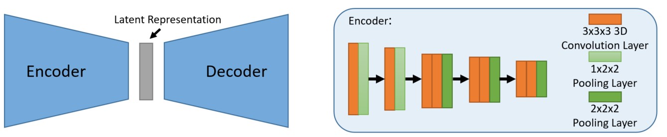
Figure 7: Our simple encoder-decoder network’s architecture. The decoder’s deconvolution layers mirror the layout of the encoder.

Our encoder-decoder network largely leverages [50]’s C3D network. As shown in Fig. 7, the encoder architecture contains the following layers (beginning from the input layer): one $3\times 3\times 3$ convolution layer with $64$ channels, one $1\times 2\times 2$ maxpool layer, one $3\times 3\times 3$ convolution layer with $128$ channels, another $1\times 2\times 2$ maxpool layer, another $3\times 3\times 3$ convolution layer with $128$ channels, one $3\times 3\times 3$ convolution layer with $256$ channels, one $2\times 2\times 2$ maxpool layer, another $3\times 3\times 3$ convolution layer with $256$ channels, one $3\times 3\times 3$ convolution layer with $512$ channels, another $2\times 2\times 2$ maxpool layer, two $3\times 3\times 3$ convolution layers with $512$ channels and another $2\times 2\times 2$ maxpool layer.

We used an initial learning rate of $1e-5$, batch size of $1$ and trained for $200$ epochs. We used Adam optimizer with default PyTorch settings. The data samples are generated by sampling a random segment during the evolution of a group for all groups in all the datasets. The data samples are normalized in scale and positions such that the entire group space sequence fits inside the $224\times 224$ image sequences and the geometric center of the group in the last input sequence frame is at the center of the image. After obtaining the predictions from the model, we filter out pixel predictions with confidence level less than $0.5$. An example is shown in Fig. 8. For evaluation on a particular dataset, including both evaluation of the encoder-decoder network’s performance and the policies in the navigation setting, we use the model that was trained on the other four datasets.

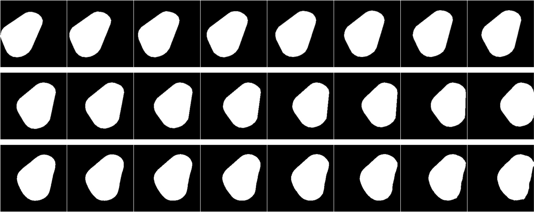
Figure 8: Top: An example group space input sequence for our encoder-decoder network. Mid: The ground truth future sequence of the group. Bottom: The predictioned future sequence of the group as outputted by our encoder-decoder network.

In simulated laser scan settings, we do not retrain the group shape prediction models. Instead, we transfer the learned group shape prediction models on perfect perception settings directly into this new setting. We use a nearest neighbor approach based on geometric centers to identify the history sequence of a group in order to predict the group’s future states. If the nearest neighbor of a group in the previous frame is more than $0.25m$ away, then we say no prior history of this group is available and use the technique in section B to linearly back-propagate the group’s history.

To integrate this encoder-decoder network into our G-MPC framework, we performed the following additional processing steps (a detailed explanation of footnote 1). Because the encoder-decoder network model takes image-based inputs, we first convert the group space convex hulls into images. We use the homography matrix provided by the dataset to convert the coordinates of the convexhull vertices from meters to pixels. Then we draw these convexhulls on empty canvases to obtain the images. We preprocessed these images to normalize the convexhulls’ sizes and positions such that these convexhulls fit inside the images throughout the input sequence and are approximately at the center of the image for the last input frame. Once we obtain the output sequence, we take the coordinates of the vertices at the edge of the output shape blobs and convert them back from pixels to meters using the inverse of the homography matrix.

D Parameter Details

For the parameters of eq. (1), we picked $\epsilon_{s},\epsilon_{\theta},\epsilon_{v}$ such that the grouping outcomes match our qualitative inspection of human grouping in the datasets similarly to our prior work [13]. For ETH, HOTEL, ZARA1 and ZARA2 we set $\epsilon_{s}=2.0m,\epsilon_{\theta}=30^{\circ},\epsilon_{v}=1.0m/s$. Because UNIV is more crowded than the other four datasets, group formations are tighter and we set $\epsilon_{s}=1.5m,\epsilon_{\theta}=15^{\circ},\epsilon_{v}=0.5m/s$.

For the parameter of eq. (17), we selected $C$ under the assumption that closely-interacting pedestrians walk around the boundaries of each other’s personal space. For ETH, HOTEL, ZARA1 and ZARA2, we set $C=0.35$. Again because UNIV has denser crowds, we set $C=0.25$. If at any given time the robot enters a social group space, we incrementally reduce $C$ by $0.1$ with a minimum value of $0.05$ until the robot is outside of the group space.

For the time horizon parameter $f$ and the history window parameter $h$ from section 4.2, we set $f=8$ and $h=8$ to ensure our MPC formulation’s compatibility with the SGAN models.

For the weight parameter $\lambda$ in the cost function in equation (10), we perform a full parameter sweep to tune $\lambda$. We test $\lambda$ with values from $0.1$ to $0.9$ with increments of $0.05$ on randomly sampled $100$ test cases. We then select $\lambda$ that results in high success rates (at least $90\%$) for both agent based and group based policies without predictions and that the success rates of the two policies are the closest to each other. For trials with non-reactive agents, we set $\lambda=0.65$. For trials with reactive agents, we set $\lambda=0.3$. Note that we want the weight parameter to be the same for both pedestrian-based and group-based policies because the distance from the pedestrians to the boundaries of the social space are the same in both settings. Keeping the same weight allows fair evaluations of these two types of policies.

For the number of control rollouts $R$ in equation (14), we set $R=12$.

E Numeric Results of Fig. 4 and Fig. 5

Table 3: Performance per scene under the Offline condition.

[0pt 2pt] Scene ETH HOTEL ZARA1 ZARA2 UNIV Task Metric Flow Cross Flow Cross Flow Cross Flow Cross Flow Cross ped-nopred $\mathcal{S}(\%)$ $91.38$ $75.86$ $95.35$ $95.45$ $96.00$ $85.71$ $97.64$ $96.90$ $83.96$ $83.33$ $\mathcal{C}(\%)$ $56.9$ $24.14$ $81.4$ $63.64$ $72.0$ $46.43$ $82.68$ $70.54$ $68.87$ $64.91$ $\mathcal{D}(m)$ $1.29$ $0.97$ $1.35$ $1.14$ $1.31$ $1.03$ $1.39$ $1.27$ $0.95$ $0.98$ $\mathcal{L}(m)$ $27.16$ $16.93$ $19.31$ $10.55$ $20.75$ $8.80$ $20.87$ $8.92$ $22.96$ $17.38$ ped-linear $\mathcal{S}(\%)$ $94.83$ $96.55$ $97.67$ $100$ $96$ $96.43$ $94.49$ $100$ $86.79$ $99.12$ $\mathcal{C}(\%)$ $75.86$ $74.14$ $86.05$ $88.64$ $84.0$ $89.29$ $88.19$ $95.35$ $79.25$ $90.35$ $\mathcal{D}(m)$ $1.42$ $1.28$ $1.28$ $1.25$ $1.53$ $1.36$ $1.53$ $1.46$ $1.01$ $1.09$ $\mathcal{L}(m)$ $27.31$ $18.08$ $19.28$ $10.72$ $20.29$ $9.48$ $20.84$ $9.16$ $22.93$ $17.06$ ped-sgan $\mathcal{S}(\%)$ $93.1$ $94.83$ $95.35$ $100$ $96$ $100$ $96.06$ $100$ $86.79$ $100$ $\mathcal{C}(\%)$ $79.31$ $70.69$ $81.4$ $79.55$ $80.0$ $92.86$ $89.76$ $95.35$ $73.58$ $86.84$ $\mathcal{D}(m)$ $1.45$ $1.27$ $1.34$ $1.23$ $1.46$ $1.35$ $1.50$ $1.47$ $0.98$ $1.08$ $\mathcal{L}(m)$ $27.05$ $17.99$ $19.20$ $10.10$ $20.51$ $9.66$ $20.83$ $9.21$ $23.05$ $17.22$ group-nopred $\mathcal{S}(\%)$ $94.83$ $87.93$ $100$ $88.64$ $92$ $75$ $96.06$ $92.25$ $93.4$ $93.86$ $\mathcal{C}(\%)$ $82.76$ $79.31$ $97.67$ $86.36$ $88.0$ $71.43$ $92.91$ $89.92$ $90.57$ $88.6$ $\mathcal{D}(m)$ $1.70$ $1.61$ $1.8$ $1.61$ $1.83$ $1.59$ $1.68$ $1.59$ $1.18$ $1.22$ $\mathcal{L}(m)$ $29.52$ $23.32$ $21.98$ $14.38$ $22.86$ $13.02$ $23.47$ $11.17$ $28.57$ $20.61$ group-pred $\mathcal{S}(\%)$ $96.55$ $86.21$ $100$ $90.91$ $96$ $82.14$ $96.85$ $94.57$ $89.62$ $93.86$ $\mathcal{C}(\%)$ $82.76$ $81.03$ $100.0$ $88.64$ $92.0$ $82.14$ $92.91$ $93.02$ $86.79$ $92.98$ $\mathcal{D}(m)$ $1.67$ $1.90$ $1.83$ $1.65$ $1.87$ $1.75$ $1.77$ $1.67$ $1.19$ $1.32$ $\mathcal{L}(m)$ $29.51$ $23.17$ $21.88$ $13.63$ $23.01$ $11.95$ $23.45$ $11.13$ $27.82$ $20.06$ laser-group-pred $\mathcal{S}(\%)$ $94.83$ $84.48$ $97.67$ $95.54$ $96$ $75$ $93.7$ $86.05$ $83.02$ $89.47$ $\mathcal{C}(\%)$ $81.03$ $82.76$ $97.67$ $90.91$ $92.0$ $75.0$ $92.13$ $86.05$ $82.08$ $85.09$ $\mathcal{D}(m)$ $1.75$ $2.21$ $1.86$ $1.70$ $1.92$ $1.81$ $1.8$ $1.76$ $1.25$ $1.40$ $\mathcal{L}(m)$ $29.57$ $23.99$ $22.42$ $15.45$ $23.50$ $12.26$ $23.63$ $11.58$ $29.49$ $22.36$

Table 4: Performance per scene under the Online condition (simulated pedestrians powered by ORCA[16]).

[0pt 2pt] Scene ETH HOTEL ZARA1 ZARA2 UNIV Task Metric Flow Cross Flow Cross Flow Cross Flow Cross Flow Cross ped-nopred $\mathcal{S}(\%)$ $96.55$ $98.28$ $100$ $97.73$ $100$ $100$ $97.64$ $100$ $88.68$ $99.12$ $\mathcal{C}(\%)$ $50.0$ $63.79$ $79.07$ $77.27$ $60.0$ $64.29$ $65.35$ $79.84$ $60.38$ $78.95$ $\mathcal{D}(m)$ $0.93$ $1.05$ $0.94$ $1.04$ $0.92$ $0.97$ $0.98$ $0.99$ $0.89$ $0.98$ $\mathcal{L}(m)$ $24.02$ $13.73$ $15.75$ $8.50$ $16.71$ $6.13$ $17.16$ $7.32$ $17.20$ $13.82$ ped-linear $\mathcal{S}(\%)$ $94.83$ $98.28$ $100$ $97.73$ $100$ $100$ $98.43$ $100$ $89.62$ $99.12$ $\mathcal{C}(\%)$ $43.1$ $70.69$ $83.72$ $90.91$ $64.0$ $85.71$ $74.8$ $80.62$ $61.32$ $88.6$ $\mathcal{D}(m)$ $0.94$ $1.04$ $0.97$ $1.03$ $0.94$ $0.99$ $0.98$ $0.99$ $0.90$ $0.98$ $\mathcal{L}(m)$ $23.83$ $13.25$ $15.43$ $8.32$ $16.54$ $6.22$ $17.03$ $6.74$ $16.87$ $13.53$ ped-sgan $\mathcal{S}(\%)$ $96.55$ $98.28$ $100$ $97.73$ $100$ $100$ $98.43$ $100$ $89.62$ $99.12$ $\mathcal{C}(\%)$ $39.66$ $63.79$ $88.37$ $88.64$ $64.0$ $82.14$ $77.95$ $82.95$ $62.26$ $86.84$ $\mathcal{D}(m)$ $0.93$ $1.04$ $0.95$ $1.04$ $0.94$ $0.99$ $0.98$ $0.99$ $0.90$ $0.98$ $\mathcal{L}(m)$ $23.85$ $13.20$ $15.63$ $8.14$ $16.54$ $6.18$ $17.06$ $6.72$ $16.90$ $13.53$ group-nopred $\mathcal{S}(\%)$ $93.1$ $98.28$ $95.35$ $100$ $96$ $100$ $97.64$ $98.45$ $89.62$ $100$ $\mathcal{C}(\%)$ $75.86$ $79.31$ $81.4$ $88.64$ $88.0$ $71.43$ $90.55$ $85.27$ $68.87$ $88.6$ $\mathcal{D}(m)$ $1.15$ $1.15$ $1.17$ $1.16$ $1.11$ $1.03$ $1.21$ $1.11$ $0.94$ $1.04$ $\mathcal{L}(m)$ $25.36$ $15.37$ $16.62$ $9.72$ $18.16$ $7.50$ $18.36$ $8.56$ $18.98$ $15.15$ group-pred $\mathcal{S}(\%)$ $94.83$ $98.28$ $97.67$ $97.73$ $92$ $96.43$ $99.21$ $99.22$ $93.4$ $98.25$ $\mathcal{C}(\%)$ $74.14$ $87.93$ $81.4$ $95.45$ $88.0$ $89.29$ $91.34$ $93.8$ $80.19$ $91.23$ $\mathcal{D}(m)$ $1.13$ $1.24$ $1.16$ $1.21$ $1.17$ $1.13$ $1.18$ $1.11$ $0.93$ $1.07$ $\mathcal{L}(m)$ $25.19$ $14.99$ $16.45$ $9.14$ $17.93$ $7.62$ $18.22$ $7.88$ $18.71$ $14.74$ laser-group-pred $\mathcal{S}(\%)$ $91.38$ $98.28$ $95.35$ $97.73$ $96$ $89.29$ $97.64$ $97.67$ $84.91$ $92.11$ $\mathcal{C}(\%)$ $70.69$ $84.48$ $88.37$ $93.18$ $88.0$ $85.71$ $88.98$ $94.57$ $60.38$ $78.07$ $\mathcal{D}(m)$ $1.18$ $1.33$ $1.26$ $1.28$ $1.18$ $1.12$ $1.23$ $1.14$ $0.93$ $1.07$ $\mathcal{L}(m)$ $25.40$ $16.27$ $16.81$ $9.82$ $18.72$ $8.54$ $19.07$ $8.57$ $21.39$ $16.46$

Tab. 3 and Tab. 4 are the numerical results of Fig. 4 and Fig. 5. $\mathcal{S}$ is the success rate. $\mathcal{C}$ is percentage of trials in which the robot does not enter any group space (collisions also count as group intrusions). $\mathcal{D}$ is the average minimum distance to pedestrians. $\mathcal{L}$ is the average path length.

References

- Thrun et al. [1999] S. Thrun, M. Bennewitz, W. Burgard, A. Cremers, F. Dellaert, D. Fox, D. Hahnel, C. Rosenberg, N. Roy, J. Schulte, and D. Schulz. MINERVA: a second-generation museum tour-guide robot. In Proceedings of the IEEE International Conference on Robotics and Automation (ICRA), volume 3, pages 1999–2005, 1999.
- Kruse et al. [2013] T. Kruse, A. K. Pandey, R. Alami, and A. Kirsch. Human-aware robot navigation: A survey. Robotics and Autonomous Systems, 61(12):1726–1743, 2013.
- Kretzschmar et al. [2016] H. Kretzschmar, M. Spies, C. Sprunk, and W. Burgard. Socially compliant mobile robot navigation via inverse reinforcement learning. The International Journal of Robotics Research, 35(11):1289–1307, 2016.
- Trautman et al. [2015] P. Trautman, J. Ma, R. M. Murray, and A. Krause. Robot navigation in dense human crowds: Statistical models and experimental studies of human-robot cooperation. International Journal of Robotics Research, 34(3):335–356, 2015.
- Mavrogiannis et al. [2019] C. I. Mavrogiannis, A. M. Hutchinson, J. Macdonald, P. Alves-Oliveira, and R. A. Knepper. Effects of distinct robotic navigation strategies on human behavior in a crowded environment. In Proceedings of the 2019 ACM/IEEE International Conference on Human-Robot Interaction (HRI ’19). ACM, 2019.
- Luber et al. [2012] M. Luber, L. Spinello, J. Silva, and K. Arras. Socially-aware robot navigation: A learning approach. In Proceedings of the IEEE/RSJ International Conference on Intelligent Robots and Systems (IROS), pages 902–907, 2012.
- Kim and Pineau [2016] B. Kim and J. Pineau. Socially adaptive path planning in human environments using inverse reinforcement learning. International Journal of Social Robotics, 8(1):51–66, 2016.
- Everett et al. [2018] M. Everett, Y. F. Chen, and J. P. How. Motion planning among dynamic, decision-making agents with deep reinforcement learning. In IEEE/RSJ International Conference on Intelligent Robots and Systems (IROS), Madrid, Spain, Sept. 2018.
- Mavrogiannis et al. [2017] C. Mavrogiannis, V. Blukis, and R. A. Knepper. Socially competent navigation planning by deep learning of multi-agent path topologies. In Proceedings of the IEEE/RSJ International Conference on Intelligent Robots and Systems (IROS), pages 6817–6824, 2017.
- Koffka [1935] K. Koffka. Principles of Gestalt psychology. Harcourt, Brace, 1935.
- Desolneux et al. [2007] A. Desolneux, L. Moisan, and J.-M. Morel. From Gestalt Theory to Image Analysis: A Probabilistic Approach. Springer Publishing Company, Incorporated, 1st edition, 2007. ISBN 0387726357.
- Vázquez and Steinfeld [2011] M. Vázquez and A. Steinfeld. An assisted photography method for street scenes. In 2011 IEEE Workshop on Applications of Computer Vision (WACV), pages 89–94, 2011.
- Wang and Steinfeld [2020] A. Wang and A. Steinfeld. Group split and merge prediction with 3D convolutional networks. IEEE Robotics and Automation Letters, 5(2):1923–1930, 2020.
- Pellegrini et al. [2009] S. Pellegrini, A. Ess, K. Schindler, and L. van Gool. You’ll never walk alone: Modeling social behavior for multi-target tracking. In Proc. IEEE Int. Conf. Comput. Vis., pages 261–268, Sept 2009.
- Lerner et al. [2007] A. Lerner, Y. Chrysanthou, and D. Lischinski. Crowds by example. Comput. Graph. Forum, 26(3):655–664, 2007.
- van den Berg et al. [2011] J. van den Berg, S. J. Guy, M. Lin, and D. Manocha. Reciprocal n-body collision avoidance. In Robotics Research, pages 3–19. Springer Berlin Heidelberg, 2011.
- Gupta et al. [2018] A. Gupta, J. Johnson, L. Fei-Fei, S. Savarese, and A. Alahi. Social GAN: Socially acceptable trajectories with generative adversarial networks. In Proceedings of the IEEE Conference on Computer Vision and Pattern Recognition (CVPR), pages 2255–2264, 2018.
- Mavrogiannis et al. [2018] C. I. Mavrogiannis, W. B. Thomason, and R. A. Knepper. Social momentum: A framework for legible navigation in dynamic multi-agent environments. In Proceedings of the 2018 ACM/IEEE International Conference on Human-Robot Interaction (HRI ’18), pages 361–369. ACM, 2018.
- Chen et al. [2019] C. Chen, Y. Liu, S. Kreiss, and A. Alahi. Crowd-robot interaction: Crowd-aware robot navigation with attention-based deep reinforcement learning. In Proceedings of the IEEE International Conference on Robotics and Automation (ICRA), pages 6015–6022, 2019.
- Zhi et al. [2021] W. Zhi, T. Lai, L. Ott, and F. Ramos. Anticipatory navigation in crowds by probabilistic prediction of pedestrian future movements. In Proceedings of the IEEE International Conference on Robotics and Automation (ICRA), 2021.
- Somani et al. [2013] A. Somani, N. Ye, D. Hsu, and W. S. Lee. Despot: Online pomdp planning with regularization. In C. J. C. Burges, L. Bottou, M. Welling, Z. Ghahramani, and K. Q. Weinberger, editors, Advances in Neural Information Processing Systems, volume 26. Curran Associates, Inc., 2013.
- Cai et al. [2021] P. Cai, Y. Luo, D. Hsu, and W. S. Lee. Hyp-despot: A hybrid parallel algorithm for online planning under uncertainty. The International Journal of Robotics Research, 40(2-3):558–573, 2021.
- Kiss et al. [2021] S. H. Kiss, K. Katuwandeniya, A. Alempijevic, and T. Vidal-Calleja. Probabilistic dynamic crowd prediction for social navigation. In 2021 IEEE International Conference on Robotics and Automation (ICRA), pages 9269–9275, 2021.
- Šochman and Hogg [2011] J. Šochman and D. C. Hogg. Who knows who - inverting the social force model for finding groups. In Proceedings of the IEEE International Conference on Computer Vision (ICCV) Workshops, pages 830–837, 2011.
- Kendon [1990] A. Kendon. Conducting interaction : Patterns of behavior in focused encounters. Studies in International Sociolinguistics, 7, 1990.
- Yang and Peters [2019] F. Yang and C. Peters. Social-aware navigation in crowds with static and dynamic groups. In 2019 11th International Conference on Virtual Worlds and Games for Serious Applications (VS-Games), pages 1–4, 2019.
- Bazzani et al. [2012] L. Bazzani, M. Cristani, and V. Murino. Decentralized particle filter for joint individual-group tracking. In Proceedings of the IEEE Conference on Computer Vision and Pattern Recognition (CVPR), pages 1886–1893, 2012.
- Chang et al. [2011] M. Chang, N. Krahnstoever, and W. Ge. Probabilistic group-level motion analysis and scenario recognition. In Proceedings of the International Conference on Computer Vision (ICCV), pages 747–754, 2011.
- Gennari and Hager [2004] G. Gennari and G. D. Hager. Probabilistic data association methods in visual tracking of groups. In Proceedings of the IEEE Computer Society Conference on Computer Vision and Pattern Recognition (CVPR), volume 2, pages II–II, 2004.
- Pellegrini et al. [2010] S. Pellegrini, A. Ess, and L. Van Gool. Improving data association by joint modeling of pedestrian trajectories and groupings. In K. Daniilidis, P. Maragos, and N. Paragios, editors, Computer Vision – ECCV 2010, pages 452–465, Berlin, Heidelberg, 2010. Springer Berlin Heidelberg. ISBN 978-3-642-15549-9.
- Zanotto et al. [2012] M. Zanotto, L. Bazzani, M. Cristani, and V. Murino. Online bayesian nonparametrics for group detection. In Proceedings of the British Machine Vision Conference (BMVC), pages 111.1–111.12, 2012.
- Chamveha et al. [2013] I. Chamveha, Y. Sugano, Y. Sato, and A. Sugimoto. Social group discovery from surveillance videos: A data-driven approach with attention-based cues. In Proceedings of the The British Machine Vision Association (BMVC), 2013.
- Khan et al. [2015] S. D. Khan, G. Vizzari, S. Bandini, and S. Basalamah. Detection of social groups in pedestrian crowds using computer vision. In S. Battiato, J. Blanc-Talon, G. Gallo, W. Philips, D. Popescu, and P. Scheunders, editors, Advanced Concepts for Intelligent Vision Systems, pages 249–260. Springer International Publishing, Cham, 2015.
- Helbing and Molnár [1995] D. Helbing and P. Molnár. Social force model for pedestrian dynamics. Physical Review E, 51(5):4282–4286, 1995.
- Mazzon et al. [2013] R. Mazzon, F. Poiesi, and A. Cavallaro. Detection and tracking of groups in crowd. In Proceedings of the IEEE International Conference on Advanced Video and Signal Based Surveillance (AVSS), pages 202–207, 2013.
- Solera et al. [2016] F. Solera, S. Calderara, and R. Cucchiara. Socially constrained structural learning for groups detection in crowd. IEEE Transactions on Pattern Analysis and Machine Intelligence, 38(5):995–1008, 2016.
- Ge et al. [2012] W. Ge, R. T. Collins, and R. B. Ruback. Vision-based analysis of small groups in pedestrian crowds. IEEE Transactions on Pattern Analysis and Machine Intelligence, 34(5):1003–1016, 2012.
- Taylor et al. [2020] A. Taylor, D. M. Chan, and L. D. Riek. Robot-centric perception of human groups. ACM Transactions on Human-Robot Interaction, 9(3):1–21, 2020.
- Chatterjee and Steinfeld [2016] I. Chatterjee and A. Steinfeld. Performance of a low-cost, human-inspired perception approach for dense moving crowd navigation. In Proceedings of the IEEE International Symposium on Robot and Human Interactive Communication (RO-MAN), pages 578–585, Aug 2016.
- Cuntoor et al. [2012] N. P. Cuntoor, R. Collins, and A. J. Hoogs. Human-robot teamwork using activity recognition and human instruction. In Proceedings of the IEEE/RSJ International Conference on Intelligent Robots and Systems (IROS), pages 459–465, 2012.
- Gockley et al. [2007] R. Gockley, J. Forlizzi, and R. Simmons. Natural person-following behavior for social robots. In Proceedings of the ACM/IEEE International Conference on Human-Robot Interaction (HRI), pages 17–24, 2007.
- Granata and Bidaud [2012] C. Granata and P. Bidaud. A framework for the design of person following behaviors for social mobile robots. In Proceedings of the IEEE/RSJ International Conference on Intelligent Robots and Systems (IROS), pages 4652–4659, 2012.
- Jung et al. [2012] E. Jung, B. Yi, and S. Yuta. Control algorithms for a mobile robot tracking a human in front. In Proceedings of the IEEE/RSJ International Conference on Intelligent Robots and Systems (IROS), pages 2411–2416, 2012.
- Zender et al. [2007] H. Zender, P. Jensfelt, and G. M. Kruijff. Human- and situation-aware people following. In Proceedings of the IEEE International Symposium on Robot and Human Interactive Communication (RO-MAN), pages 1131–1136, 2007.
- Nanavati et al. [2019] A. Nanavati, X. Z. Tan, J. Connolly, and A. Steinfeld. Follow the robot: Modeling coupled human-robot dyads during navigation. In 2019 IEEE/RSJ International Conference on Intelligent Robots and Systems (IROS), pages 3836–3843, 2019.
- Feil-Seifer and Matarić [2011] D. Feil-Seifer and M. Matarić. People-aware navigation for goal-oriented behavior involving a human partner. In Proceedings of the IEEE International Conference on Development and Learning (ICDL), volume 2, pages 1–6, 2011.
- Pandey and Alami [2009] A. K. Pandey and R. Alami. A step towards a sociable robot guide which monitors and adapts to the person’s activities. In 2009 International Conference on Advanced Robotics, pages 1–8, 2009.
- Garrell and Sanfeliu [2010] A. Garrell and A. Sanfeliu. Local optimization of cooperative robot movements for guiding and regrouping people in a guiding mission. In Proceedings of the IEEE/RSJ International Conference on Intelligent Robots and Systems (IROS), pages 3294–3299, 2010.
- Shiomi et al. [2007] M. Shiomi, T. Kanda, S. Koizumi, H. Ishiguro, and N. Hagita. Group attention control for communication robots with wizard of oz approach. In Proceedings of the ACM/IEEE International Conference on Human-Robot Interaction (HRI), pages 121–128, 2007.
- Martinez-Garcia et al. [2005] E. A. Martinez-Garcia, Ohya Akihisa, and Shin’ichi Yuta. Crowding and guiding groups of humans by teams of mobile robots. In Proceedings of the IEEE Workshop on Advanced Robotics and its Social Impacts (ARSO), pages 91–96, 2005.
- Katyal et al. [2020] K. Katyal, Y. Gao, J. Markowitz, I.-J. Wang, and C.-M. Huang. Group-Aware Robot Navigation in Crowded Environments. arXiv e-prints, art. arXiv:2012.12291, Dec. 2020.
- Ester et al. [1996] M. Ester, H.-P. Kriegel, J. Sander, and X. Xu. A density-based algorithm for discovering clusters a density-based algorithm for discovering clusters in large spatial databases with noise. In Proc. Int. Conf. Knowl. Discovery and Data Mining, pages 226–231, 1996.
- Kirby [2010] R. Kirby. Social Robot Navigation. PhD thesis, Carnegie Mellon University, Pittsburgh, PA, May 2010.
- Tran et al. [2015] D. Tran, L. Bourdev, R. Fergus, L. Torresani, and M. Paluri. Learning spatiotemporal features with 3d convolutional networks. In Proc. IEEE Int. Conf. Comput. Vis., December 2015.
- Alahi et al. [2016] A. Alahi, K. Goel, V. Ramanathan, A. Robicquet, L. Fei-Fei, and S. Savarese. Social LSTM: Human trajectory prediction in crowded spaces. In Proceedings of the IEEE Conference on Computer Vision and Pattern Recognition (CVPR), pages 961–971, 2016.
- Zhang et al. [2019] P. Zhang, W. Ouyang, P. Zhang, J. Xue, and N. Zheng. Sr-lstm: State refinement for lstm towards pedestrian trajectory prediction. In Proc. IEEE Comput. Soc. Conf. Comput. Vis. Pattern Recognit., pages 12085–12094, June 2019.
- Cao et al. [2019] C. Cao, P. Trautman, and S. Iba. Dynamic channel: A planning framework for crowd navigation. In 2019 International Conference on Robotics and Automation (ICRA), pages 5551–5557, 2019.
- Biswas et al. [2021] A. Biswas, A. Wang, G. Silvera, A. Steinfeld, and H. Admoni. Socnavbench: A grounded simulation testing framework for evaluating social navigation. arXiv preprint arXiv:2103.00047, 2021.
- Mavrogiannis et al. [2021] C. Mavrogiannis, F. Baldini, A. Wang, D. Zhao, P. Trautman, A. Steinfeld, and J. Oh. Core Challenges of Social Robot Navigation: A Survey. arXiv e-prints, art. arXiv:2103.05668, Mar. 2021.
- Schöller et al. [2020] C. Schöller, V. Aravantinos, F. Lay, and A. Knoll. What the constant velocity model can teach us about pedestrian motion prediction. IEEE Robotics and Automation Letters, 5(2):1696–1703, 2020.
- Guen and Thome [2020] V. L. Guen and N. Thome. Disentangling physical dynamics from unknown factors for unsupervised video prediction. In Proceedings of the IEEE/CVF Conference on Computer Vision and Pattern Recognition (CVPR), June 2020.