Clustering by Maximizing Mutual Information Across Views

Abstract

We propose a novel framework for image clustering that incorporates joint representation learning and clustering. Our method consists of two heads that share the same backbone network - a “representation learning” head and a “clustering” head. The “representation learning” head captures fine-grained patterns of objects at the instance level which serve as clues for the “clustering” head to extract coarse-grain information that separates objects into clusters. The whole model is trained in an end-to-end manner by minimizing the weighted sum of two sample-oriented contrastive losses applied to the outputs of the two heads. To ensure that the contrastive loss corresponding to the “clustering” head is optimal, we introduce a novel critic function called “log-of-dot-product”. Extensive experimental results demonstrate that our method significantly outperforms state-of-the-art single-stage clustering methods across a variety of image datasets, improving over the best baseline by about 5-7% in accuracy on CIFAR10/20, STL10, and ImageNet-Dogs. Further, the “two-stage” variant of our method also achieves better results than baselines on three challenging ImageNet subsets.

1 Introduction

The explosion of unlabeled data, especially visual content in recent years has led to the growing demand for effective organization of these data into semantically distinct groups in an unsupervised manner. Such data clustering facilitates downstream machine learning and reasoning tasks. Since labels are unavailable, clustering algorithms are mainly based on the similarity between samples to predict the cluster assignment. However, common similarity metrics such as cosine similarity or (negative) Euclidean distance are ineffective when applied to high-dimensional data like images. Modern image clustering methods [7, 19, 20, 43, 46, 47], therefore, leverage deep neural networks (e.g., CNNs, RNNs) to transform high-dimensional data into low-dimensional representation vectors in the latent space and perform clustering in that space. Ideally, a good clustering model assigns data to clusters to keep inter-group similarity low while maintaining high intra-group similarity. Most existing deep clustering methods do not satisfy both of these properties. For example, autoencoder-based clustering methods [21, 46, 48] often learn representations that capture too much information including distracting information like background or texture. This prevents them from computing proper similarity scores between samples at the cluster-level. Autoencoder-based methods have only been tested on simple image datasets like MNIST. Another class of methods [7, 19, 20] directly use cluster-assignment probabilities rather than representation vectors to compute the similarity between samples. These methods can only differentiate objects belonging to different clusters but not in the same cluster, hence, may incorrectly group distinct objects into the same cluster. This leads to low intra-group similarity.

To address the limitations of existing methods, we propose a novel framework for image clustering called Contrastive Representation Learning and Clustering (CRLC). CRLC consists of two heads sharing the same backbone network: a “representation learning” head (RL-head) that outputs a continuous feature vector, and a “clustering” head (C-head) that outputs a cluster-assignment probability vector. The RL-head computes the similarity between objects at the instance level while the C-head separates objects into different clusters. The backbone network serves as a medium for information transfer between the two heads, allowing the C-head to leverage disciminative fine-grained patterns captured by the RL-head to extract correct coarse-grained cluster-level patterns. Via the two heads, CRLC can effectively modulate the inter-cluster and intra-cluster similarities between samples. CRLC is trained in an end-to-end manner by minimizing a weighted sum of two sample-oriented contrastive losses w.r.t. the two heads. To ensure that the contrastive loss corresponding to the C-head leads to the tightest InfoNCE lower bound [35], we propose a novel critic called “log-of-dot-product” to be used in place of the conventional “dot-product” critic.

In our experiments, we show that CRLC significantly outperforms a wide range of state-of-the-art single-stage clustering methods on five standard image clustering datasets including CIFAR10/20, STL10, ImageNet10/Dogs. The “two-stage” variant of CRLC also achieves better results than SCAN - a powerful two-stage clustering method on three challenging ImageNet subsets with 50, 100, and 200 classes. When some labeled data are provided, CRLC, with only a small change in its objective, can surpass many state-of-the-art semi-supervised learning algorithms by a large margin.

In summary, our main contributions are:

1. A novel framework for joint representation learning and clustering trained via two sample-oriented contrastive losses on feature and probability vectors;

2. An optimal critic for the contrastive loss on probability vectors; and,

3. Extensive experiments and ablation studies to validate our proposed method against baselines.

2 Preliminaries

2.1 Representation learning by maximizing mutual information across different views

Maximizing mutual information across different views (or ViewInfoMax for short) allows us to learn view-invariant representations that capture the semantic information of data important for downstream tasks (e.g., classification). This learning strategy is also the key factor behind recent successes in representation learning [18, 33, 39, 42].

Since direct computation of mutual information is difficult [29, 37], people usually maximize the variational lower bounds of mutual information instead. The most common lower bound is InfoNCE [35] whose formula is given by:

$$I(X,\tilde{X}) \geq I_{\text{InfoNCE}}(X,\tilde{X})$$ (1)

$$\triangleq\mathbb{E}_{p(x_{1:M})p(\tilde{x}|x_{1})}\left[\log\frac{e^{f(\tilde{x},x_{1})}}{\sum_{i=1}^{M}e^{f(\tilde{x},x_{i})}}\right]+\log M$$ (2)

$$=-\mathcal{L}_{\text{contrast}}+\log M$$ (3)

where $X$, $\tilde{X}$ denote random variables from 2 different views. $x_{1:M}$ are $M$ samples from $p_{X}$, $\tilde{x}$ is a sample from $p_{\tilde{X}}$ associated with $x_{1}$. $(\tilde{x},x_{1})$ is called a “positive” pair and $(\tilde{x},x_{i})$ ($i=2,...,M$) are called “negative” pairs. $f(x,y)$ is a real value function called “critic” that characterizes the similarity between $x$ and $y$. $\mathcal{L}_{\text{contrast}}$ is often known as the “contrastive loss” in other works [8, 39].

Since $\log\frac{e^{f(\tilde{x},x_{1})}}{\sum_{i=1}^{M}e^{f(\tilde{x},x_{i})}}\leq 0$, $I_{\text{InfoNCE}}(X,\tilde{X})$ is upper-bounded by $\log M$. It means that: i) the InfoNCE bound is very loose if $I(X,\tilde{X})\gg\log M$, and ii) by increasing $M$, we can achieve a better bound. Despite being biased, $I_{\text{InfoNCE}}(X,\tilde{X})$ has much lower variance than other unbiased lower bounds of $I(X,\tilde{X})$ [35], which allows stable training of models.

Implementing the critic

In practice, $f(\tilde{x},x_{i})$ is implemented as the scaled cosine similarity between the representations of $\tilde{x}$ and $x_{i}$ as follows:

$$f(\tilde{x},x_{i}) =f(\tilde{z},z_{i})=\tilde{z}^{\top}z_{i}/\tau$$ (4)

where $\tilde{z}$ and $z_{i}$ are unit-normed representation vectors of $\tilde{x}$ and $x_{i}$, respectively; $\left\|\tilde{z}\right\|_{2}=\left\|z_{i}\right\|_{2}=1$. $\tau>0$ is the “temperature” hyperparameter. Interestingly, $f$ in Eq. 4 matches the theoretically optimal critic that leads to the tightest InfoNCE bound for unit-normed representation vectors (detailed explanation in Appdx. A.4)

In Eq. 4, we use $f(\tilde{z},z_{i})$ instead of $f(\tilde{x},x_{i})$ to emphasize that the critic $f$ in this context is a function of representations. In regard to this, we rewrite the contrastive loss in Eq. 3 as follows:

$$\mathcal{L}_{\text{FC}} =\mathbb{E}_{p(x_{1:M})p(\tilde{x}|x_{1})}\left[-\log\frac{e^{f(\tilde{z},z_{1})}}{\sum_{i=1}^{M}e^{f(\tilde{z},z_{i})}}\right]$$ (5)

$$=\mathbb{E}_{p(x_{1:M})p(\tilde{x}|x_{1})}\left[\tilde{z}^{\top}z_{1}/\tau-\log\sum_{i=1}^{M}\exp(\tilde{z}^{\top}z_{i}/\tau)\right]$$ (6)

where FC stands for “feature contrastive”.

3 Method

3.1 Clustering by maximizing mutual information across different views

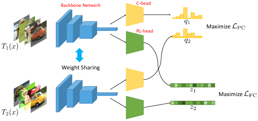
Figure 1: Overview of our proposed framework for Contrastive Representation Learning and Clustering (CRLC). Our framework consists of a “clustering” head and a “representation learning” head sharing the same backbone network. $x$ denotes an input images and $T_{1}(x)$, $T_{2}(x)$ denote two different transformations of $x$.

In the clustering problem, we want to learn a parametric classifier $s_{\theta}$ that maps each unlabeled sample $x_{i}$ to a cluster-assignment probability vector $q_{i}=(q_{i,1},...,q_{i,C})$ ($C$ is the number of clusters) whose component $q_{i,c}$ characterizes how likely $x_{i}$ belongs to the cluster $c$ ($c\in\{1,...,C\}$). Intuitively, we can consider $q_{i}$ as a representation of $x_{i}$ and use this vector to capture the cluster-level information in $x_{i}$ by leveraging the “ViewInfoMax” idea discussed in Section 1. It leads to the following loss for clustering:

$$\mathcal{L}_{\text{cluster}} =\mathbb{E}_{p(x_{1:M})p(\tilde{x}|x_{1})}\left[-\log\frac{e^{f(\tilde{q},q_{1})}}{\sum_{i=1}^{M}e^{f(\tilde{q},q_{i})}}\right]-\lambda H(\tilde{Q}_{\text{avg}})$$ (7)

$$=\mathcal{L}_{\text{PC}}-\lambda H(\tilde{Q}_{\text{avg}})$$ (8)

where $\lambda\geq 0$ is a coefficient; $\tilde{q}$, $q_{i}$ are probability vectors associated with $\tilde{x}$ and $x_{i}$, respectively. $\mathcal{L}_{\text{PC}}$ is the probability contrastive loss similar to $\mathcal{L}_{\text{FC}}$ (Eq. 5) but with feature vectors replaced by probability vectors. $H$ is the entropy of the marginal cluster-assignment probability $\tilde{q}_{\text{avg}}=\mathbb{E}_{p(x_{1})p(\tilde{x}|x_{1})}\left[\tilde{q}\right]$. Here, we maximize $H(\tilde{Q}_{\text{avg}})$ to avoid a degenerate solution in which all samples fall into the same cluster (e.g., $\tilde{q}$ is one-hot for all samples). However, it is free to use other regularizers on $\tilde{q}_{\text{avg}}$ rather than $-H(\tilde{Q}_{\text{avg}})$.

Choosing a suitable critic

It is possible to use the conventional “dot-product” critic for $\mathcal{L}_{\text{PC}}$ as for $\mathcal{L}_{\text{FC}}$ (Eq. 4). However, this will lead to suboptimal results (Section 5.3) since $\mathcal{L}_{\text{PC}}$ is applied to categorical probability vectors rather than continuous feature vectors. Therefore, we need to choose a suitable critic for $\mathcal{L}_{\text{PC}}$ so that the InfoNCE bound associated with $\mathcal{L}_{\text{PC}}$ is tightest. Ideally, $f(\tilde{x},x_{i})$ should match the theoretically optimal critic $f^{*}(\tilde{x},x_{i})$ which is proportional to $\log p(\tilde{x}|x_{i})$ (detailed explanation in Appdx. A.3). Denoted by $\tilde{y}$ and $y_{i}$ the cluster label of $\tilde{x}$ and $x_{i}$ respectively, we then have:

$$\log p(\tilde{x}|x_{i}) \approx\log\sum_{c=1}^{C}p(\tilde{y}=c|y_{i}=c)$$

$$\propto\log\sum_{c=1}^{C}\tilde{q}_{c}q_{i,c}=\log(\tilde{q}^{\top}q_{i})$$ (9)

Thus, the most suitable critic is $f(\tilde{q},q_{i})=\log(\tilde{q}^{\top}q_{i})$ which we refer to as the “log-of-dot-product” critic. This critic achieves its maximum value when $\tilde{q}$ and $q_{i}$ are the same one-hot vectors and its minimum value when $\tilde{q}$ and $q_{i}$ are different one-hot vectors. Apart from this critic, we also list other nonoptimal critics in Appdx. A.1. Empirical comparison of the “log-of-dot-product” critic with other critics is provided in Section 5.3.

In addition, to avoid the gradient saturation problem of minimizing $\mathcal{L}_{\text{PC}}$ when probabilities are close to one-hot (explanation in Appdx. A.5), we smooth out the probabilities as follows:

$$q=(1-\gamma)q+\gamma r$$

where $r=\left(\frac{1}{C},...,\frac{1}{C}\right)$ is the uniform probability vector over $C$ classes; $0\leq\gamma\leq 1$ is the smoothing coefficient set to 0.01 if not otherwise specified.

Implementing the contrastive probability loss

To implement $\mathcal{L}_{\text{PC}}$, we can use either the SimCLR framework [8] or the MemoryBank framework [42]. If the SimCLR framework is chosen, both $\tilde{q}$ and $q_{i}$ ($i\in\{1,...,M\}$) are computed directly from $\tilde{x}$ and $x_{i}$ respectively via the parametric classifier $s_{\theta}$. On the other hand, if the MemoryBank framework is chosen, we maintain a nonparametric memory bank $\mathcal{M}$ - a matrix of size $N\times C$ containing the cluster-assignment probabilities of all $N$ training samples, and update its rows once a new probability is computed as follows:

$$q_{n,t+1}=\alpha q_{n,t}+(1-\alpha)\hat{q}_{n}$$ (10)

where $\alpha$ is the momentum, which is set to 0.5 in our work if not otherwise specified; $q_{n,t}$ is the probability vector of the training sample $x_{n}$ at step $t$ corresponding to the $n$-th row of $\mathcal{M}$; $\hat{q}_{n}=s_{\theta}(x_{n})$ is the new probability vector. Then, except $\tilde{q}$ computed via $s_{\theta}$ as normal, all $q_{i}$ in Eq. 7 are sampled uniformly from $\mathcal{M}$. At step 0, all the rows of $\mathcal{M}$ are initialized with the same probability of $\left(\frac{1}{C},...,\frac{1}{C}\right)$. We also tried implementing $\mathcal{L}_{\text{PC}}$ using the MoCo framework [16] but found that it leads to unstable training. The main reason is that during the early stage of training, the EMA model in MoCo often produces inconsistent cluster-assignment probabilities for different views.

3.2 Incorporating representation learning

Due to the limited representation capability of categorical probability vectors, models trained by minimizing the loss $\mathcal{L}_{\text{cluster}}$ in Eq.7 are not able to discriminate objects in the same cluster. Thus, they may capture suboptimal cluster-level patterns, which leads to unsatisfactory results.

To overcome this problem, we propose to combine clustering with contrastive representation learning into a unified framework called CRLC. As illustrated in Fig. 1, CRLC consists of a “clustering” head (C-head) and a “representation learning” head (RL-head) sharing the same backbone network. The backbone network is usually a convolutional neural network which maps an input image $x$ into a hidden vector $h$. Then, $h$ is fed to the C-head and the RL-head to produce a cluster-assignment probability vector $q$ and a continuous feature vector $z$, respectively. We simultaneously apply the clustering loss $\mathcal{L}_{\text{cluster}}$ (Eq. 8) and the feature contrastive loss $\mathcal{L}_{\text{FC}}$ (Eq. 6) on $q$ and $z$ respectively and train the whole model with the weighted sum of $\mathcal{L}_{\text{cluster}}$ and $\mathcal{L}_{\text{FC}}$ as follows:

$$\mathcal{L}_{\text{\text{CRLC}}} =\mathcal{L}_{\text{cluster}}+\lambda\mathcal{L}_{\text{FC}}$$

$$=\mathcal{L}_{\text{PC}}-\lambda_{1}H(\tilde{Q}_{\text{avg}})+\lambda_{2}\mathcal{L}_{\text{FC}}$$ (11)

where $\lambda_{1},\lambda_{2}\geq 0$ are coefficients.

3.3 A simple extension to semi-supervised learning

Although CRLC is originally proposed for unsupervised clustering, it can be easily extended to semi-supervised learning (SSL). There are numerous ways to adjust CRLC so that it can incorporate labeled data during training. However, within the scope of this work, we only consider a simple approach which is adding a crossentropy loss on labeled data to $\mathcal{L}_{\text{CRLC}}$. The new loss is given by:

$$\mathcal{L}_{\text{CRLC-semi}} =\mathcal{L}_{\text{CRLC}}+\lambda\mathbb{E}_{(x_{l},y_{l})\sim\mathcal{D}_{l}}\left[-\log p(y_{l}|x_{l})\right]$$

$$=\mathcal{L}_{\text{PC}}-\lambda_{1}H(\tilde{Q}_{\text{avg}})+\lambda_{2}\mathcal{L}_{\text{FC}}+\lambda_{3}\mathcal{L}_{\text{xent}}$$ (12)

We call this variant of CRLC “CRLC-semi”. Despite its simplicity, we will empirically show that CRLC-semi outperforms many state-of-the-art SSL methods when only few labeled samples are available. We conjecture that the clustering objective arranges the data into disjoint clusters, making classification easier.

4 Related Work

There are a large number of clustering and representation learning methods in literature. However, within the scope of this paper, we only discuss works in two related topics, namely, contrastive learning and deep clustering.

4.1 Contrastive Learning

Despite many recent successes in learning representations, the idea of contrastive learning appeared long time ago. In 2006, Hadsell et. al. [15] proposed a max-margin contrastive loss and linked it to a mechanical spring system. In fact, from a probabilistic view, contrastive learning arises naturally when working with energy-based models. For example, in many problems, we want to maximize $\log p(y|x)=\log\frac{e^{f(y,x))}}{\sum_{y^{\prime}\in\mathcal{Y}}e^{f(y^{\prime},x)}}$ where $y$ is the output associated with a context $x$ and $\mathcal{Y}$ is the set of all possible outputs or vocab. This is roughly equivalent to maximizing $f(y,x)$ and minimizing $f(y^{\prime},x)$ for all $y^{\prime}\neq y$ but in a normalized setting. However, in practice, the size of $\mathcal{Y}$ is usually very large, making the computation of $p(y|x)$ expensive. This problem was addressed in [32, 42] by using Noise Contrastive Estimation (NCE) [14] to approximate $p(y|x)$. The basic idea of NCE is to transform the density estimation problem into a binary classification problem: “Whether samples are drawn from the data distribution or from a known noise distribution?”. Based on NCE, Mikolov et. al. [30] and Oord et. al. [33] derived a simpler contrastive loss which later was referred to as the InfoNCE loss [35] and was adopted by many subsequent works [8, 12, 16, 31, 39, 49] for learning representations.

Recently, there have been several attempts to leverage inter-sample statistics obtained from clustering to improve representation learning on a large scale [1, 4, 54]. PCL [26] alternates between clustering data via K-means and contrasting samples based on their views and their assigned cluster centroids (or prototypes). SwAV [5] does not contrast two sample views directly but uses one view to predict the code of assigning the other view to a set of learnable prototypes. InterCLR [44] and ODC [51] avoid offline clustering on the entire training dataset after each epoch by storing a pseudo-label for every sample in the memory bank (along with the feature vector) and maintaining a set of cluster centroids. These pseudo-labels and cluster centroids are updated on-the-fly at each step via mini-batch K-means.

4.2 Deep Clustering

Traditional clustering algorithms such as K-means or Gaussian Mixture Model (GMM) are mainly designed for low-dimensional vector-like data, hence, do not perform well on high-dimensional structural data like images. Deep clustering methods address this limitation by leveraging the representation power of deep neural networks (e.g., CNNs, RNNs) to effectively transform data into low-dimensional feature vectors which are then used as inputs for a clustering objective. For example, DCN [46] applies K-means to the latent representations produced by an auto-encoder. The reconstruction loss and the K-means clustering loss are minimized simultaneously. DEC [43], by contrast, uses only an encoder rather than a full autoencoder like DCN to compute latent representations. This encoder and the cluster centroids are learned together via a clustering loss proposed by the authors. JULE [47] uses a RNN to implement agglomerative clustering on top of the representations outputted by a CNN and trains the two networks in an end-to-end manner. VaDE [21] regards clustering as an inference problem and learns the cluster-assignment probabilities of data using a variational framework [22]. Meanwhile, DAC [7] treats clustering as a binary classification problem: “Whether a pair of samples belong to the same cluster or not?”. To obtain a pseudo label for a pair, the cosine similarity between the cluster-assignment probabilities of the two samples in that pair is compared with an adaptive threshold. IIC [20] learns cluster assignments via maximizing the mutual information between clusters under two different data augmentations. PICA [19], instead, minimizes the contrastive loss derived from the the mutual information in IIC. While the cluster contrastive loss in PICA is cluster-oriented and can have at most $C$ negative pairs ($C$ is the number of clusters). Our probability contrastive loss, by contrast, is sample-oriented and can have as many negative pairs as the number of training data. Thus, in theory, our proposed model can capture more information than PICA. In real implementation, in order to gain more information from data, PICA has to make use of the “over-clustering” trick [20]. It alternates between minimizing $\mathcal{L}_{\text{PICA}}$ for $C$ clusters and minimizing $\mathcal{L}_{\text{PICA}}$ for $kC$ clusters ($k>1$ denotes the “over-clustering” coefficient). DRC [53] and CC [27] enhances PICA by combining clustering with contrastive representation learning, which follows the same paradigm as our proposed CRLC. However, like PICA, DRC and CC uses cluster-oriented representations rather than sample-oriented representations.

In addition to end-to-end deep clustering methods, some multi-stage clustering methods have been proposed recently [34, 40]. The most notable one is SCAN [40]. This method uses representations learned via contrastive learning during the first stage to find nearest neighbors for every sample in the training set. In the second stage, neighboring samples are forced to have similar cluster-assignment probabilities. Our probability contrastive loss can easily be extended to handle neighboring samples (see Section 5.1.2).

5 Experiments

Dataset	CIFAR10			CIFAR20			STL10			ImageNet10			ImageNet-Dogs
Metric	ACC	NMI	ARI	ACC	NMI	ARI	ACC	NMI	ARI	ACC	NMI	ARI	ACC	NMI	ARI
JULE [47]	27.2	19.2	13.8	13.7	10.3	3.3	27.7	18.2	16.4	30.0	17.5	13.8	13.8	5.4	2.8
DEC [43]	30.1	25.7	16.1	18.5	13.6	5.0	35.9	27.6	18.6	38.1	28.2	20.3	19.5	12.2	7.9
DAC [7]	52.2	39.6	30.6	23.8	18.5	8.8	47.0	36.6	25.7	52.7	39.4	30.2	27.5	21.9	11.1
DDC [6]	52.4	42.4	32.9	-	-	-	48.9	37.1	26.7	57.7	43.3	34.5	-	-	-
DCCM [41]	62.3	49.6	40.8	32.7	28.5	17.3	48.2	37.6	26.2	70.1	60.8	55.5	38.3	32.1	18.2
IIC [20]	61.7	-	-	25.7	-	-	61.0	-	-	-	-	-	-	-	-
MCR2 [50]	68.4	63.0	50.8	34.7	36.2	16.7	49.1	44.6	29.0	-	-	-	-	-	-
PICA [19]	69.6	59.1	51.2	33.7	31.0	17.1	71.3	61.1	53.1	87.0	80.2	76.1	35.2	35.2	20.1
DRC [53]	72.7	62.1	54.7	36.7	35.6	20.8	74.7	64.4	56.9	88.4	83.0	79.8	38.9	38.4	23.3
C-head only	66.9	56.9	47.5	37.7	35.7	21.6	61.2	52.7	43.4	80.0	75.2	67.6	36.3	37.5	19.8
CRLC	79.9	67.9	63.4	42.5	41.6	26.3	81.8	72.9	68.2	85.4	83.1	75.9	46.1	48.4	29.7

Table 1: End-to-end clustering results on 5 standard image datasets. Due to space limit, we only show the means of the results. For the standard deviations, please refer to Appdx. A.8.

ImageNet	50 classes				100 classes				200 classes
Metric	ACC	ACC5	NMI	ARI	ACC	ACC5	NMI	ARI	ACC	ACC5	NMI	ARI
K-means [40]	65.9	-	77.5	57.9	59.7	-	76.1	50.8	52.5	-	75.5	43.2
SCAN [40]	75.1	91.9	80.5	63.5	66.2	88.1	78.7	54.4	56.3	80.3	75.7	44.1
two-stage CRLC	75.4	93.3	80.6	63.4	66.7	88.3	79.2	55.0	57.9	80.6	76.4	45.9

Table 2: Two-stage clustering results on ImageNet50/100/200.

Dataset

We evaluate our proposed method on 5 standard datasets for image clustering which are CIFAR10/20 [23], STL10 [9], ImageNet10 [11, 7], and ImageNet-Dogs [11, 7], and on 3 big ImageNet subsets namely ImageNet50/100/200 with 50/100/200 classes, respectively [11, 40]. A description of these datasets is given in Appdx. A.6. Our data augmentation setting follows [16, 42]. We first randomly crop images to a desirable size (32$\times$32 for CIFAR, 96$\times$96 for STL10, and 224$\times$224 for ImageNet subsets). Then, we perform random horizontal flip, random color jittering, and random grayscale conversion. For datasets which are ImageNet subsets, we further apply Gaussian blurring at the last step [8]. Similar to previous works [7, 20, 19], both the training and test sets are used for CIFAR10, CIFAR20 and STL10 while only the training set is used for other datasets. We also provide results where only the training set is used for CIFAR10, CIFAR20 and STL10 in Appdx. A.8. For STL10, 100,000 auxiliary unlabeled samples are additionally used to train the “representation learning” head. However, when training the “clustering” head, these auxiliary samples are not used since their classes may not appear in the training set.

Model architecture and training setups

Following previous works [19, 20, 40, 53], we adopt ResNet34 and ResNet50 [17] as the backbone network when working on the 5 standard datasets and on the 3 big ImageNet subsets, respectively. The “representation learning” head (RL-head) and the “clustering” head (C-head) are two-layer neural networks with ReLU activations. The length of the output vector of the RL-head is 128. The temperature $\tau$ (Eq. 5) is fixed at 0.1. To reduce variance in learning, we train our model with 10 C-subheads similar to [20]. This only adds little extra computation to our model. However, unlike [19, 20, 53], we do not use an auxiliary “over-clustering” head to exploit additional information from data since we think our RL-head can do that effectively.

Training setups for end-to-end and two-stage clustering are provided in Appdx. A.7.

Evaluation metrics

We use three popular clustering metrics namely Accuracy (ACC), Normalized Mutual Information (NMI), Adjusted Rand Index (ARI) for evaluation. For unlabeled data, ACC is computed via the Kuhn-Munkres algorithm. All of these metrics scale from 0 to 1 and higher values indicate better performance. In this work, we convert the [0, 1] range into percentage.

5.1 Clustering

5.1.1 End-to-end training

Table 1 compares the performance of our proposed CRLC with a wide range of state-of-the-art deep clustering methods. CRLC clearly outperforms all baselines by a large margin on most datasets. For example, in term of clustering accuracy (ACC), our method improves over the best baseline (DRC [53]) by 5-7% on CIFAR10/20, STL10, and ImageNet-Dogs. Gains are even larger if we compare with methods that do not explicitly learn representations such as PICA [19] and IIC [20]. CRLC only performs worse than DRC on ImageNet10, which we attribute to our selection of hyperparameters. In addition, even when only the “clustering” head is used, our method still surpasses most of the baselines (e.g., DCCM, IIC). These results suggest that: i) we can learn semantic clusters from data just by minimizing the probability contrastive loss, and ii) combining with contrastive representation learning improves the quality of the cluster assignment.

To have a better insight into the performance of CRLC, we visualize some success and failure cases in Fig. 2 (and also in Appdx. A.11). We see that samples predicted correctly with high confidence are usually representative for the cluster they belong to. It suggests that CRLC has learned coarse-grained patterns that separate objects at the cluster level. Besides, CRLC has also captured fine-grained instance-level information, thus, is able to find nearest neighbors with great similarities in shape, color and texture to the original image. Another interesting thing from Fig. 2 is that the predicted label of a sample is often strongly correlated with that of the majority of its neighbors. It means that: i) CRLC has learned a smooth mapping from images to cluster assignments, and ii) CRLC tends to make “collective” errors (the first and third rows in Fig. 2c). Other kinds of errors may come from the closeness between classes (e.g., horse vs. dog), or from some adversarial signals in the input (e.g., the second row in Fig. 2b). Solutions for fixing these errors are out of scope of this paper and will be left for future work.

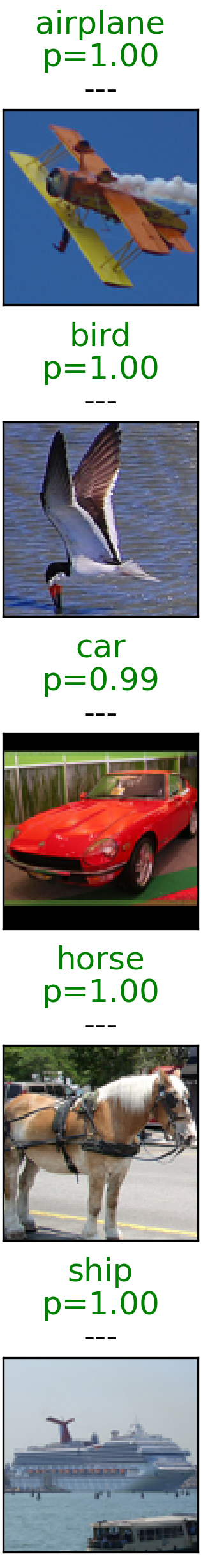
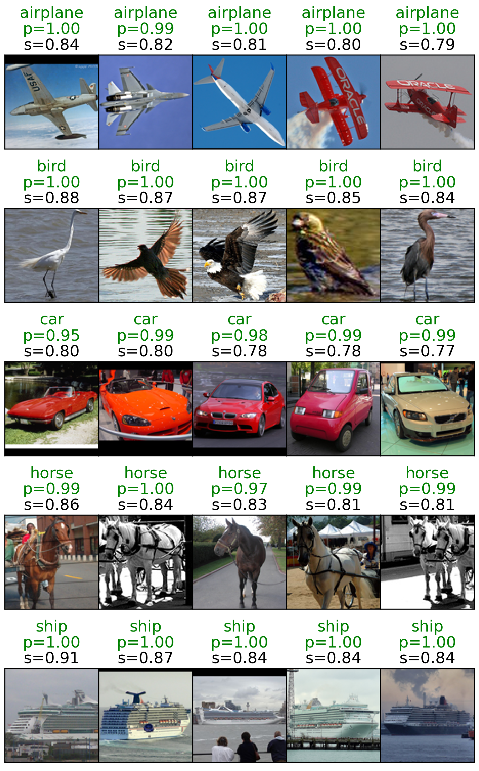
(a) correct

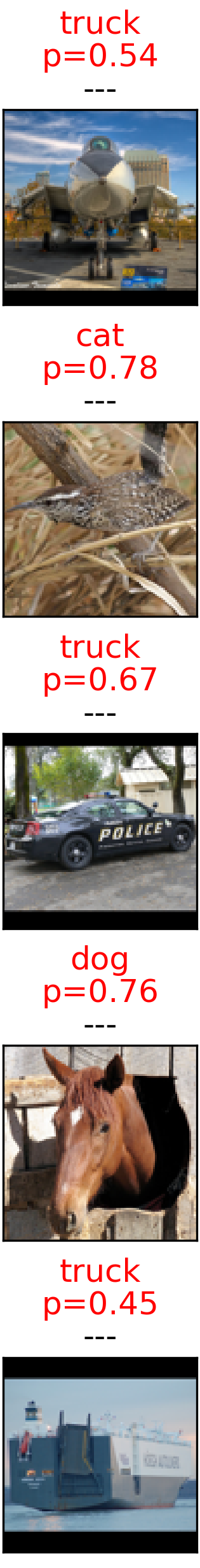
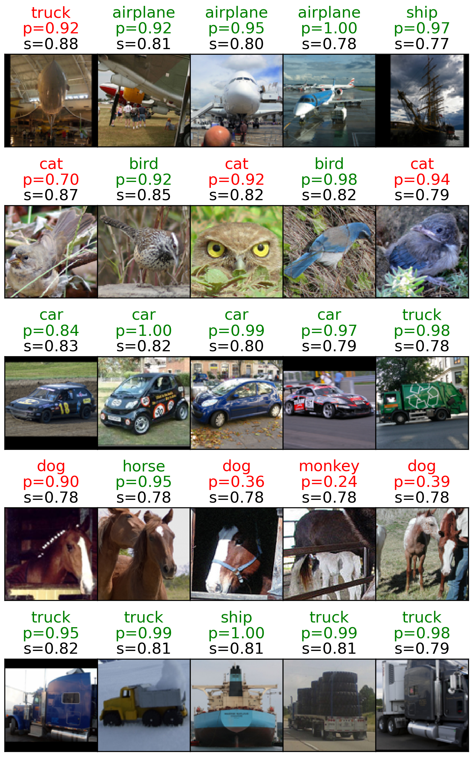
(b) false negative

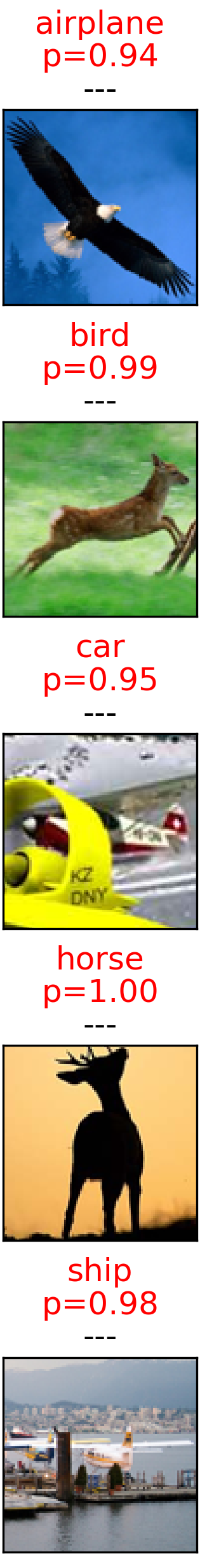
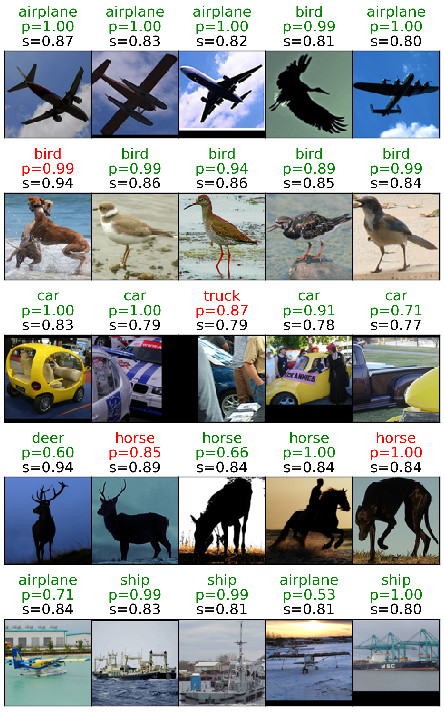
(c) false positive

Figure 2: STL10 samples of 5 classes correctly (green) and incorrectly (red) predicted by CRLC. For each subplot, we show reference samples on the leftmost column and their nearest neighbors on the right. Neighbors are retrieved based on the normalized cosine similarity (“s”) between the feature vectors of two samples. “p” denotes the confidence probability.

5.1.2 Two-stage training

Although CRLC is originally proposed as an end-to-end clustering algorithm, it can be easily extended to a two-stage clustering algorithm similar to SCAN [40]. To do that, we first pretrain the RL-head and the backbone network with $\mathcal{L}_{\text{FC}}$ (Eq. 6). Next, for every sample in the training data, we find a set of $K$ nearest neighbors based on the cosine similarity between feature vectors produced by the pretrained network. In the second stage, we train the C-head by minimizing $\mathcal{L}_{\text{cluster}}$ (Eq. 8) with the positive pair consisting of a sample and its neighbor drawn from a set of $K$ nearest neighbors. We call this variant of CRLC “two-stage” CRLC. In fact, we did try training both the C-head and the RL-head in the second stage by minimizing $\mathcal{L}_{\text{CRLC}}$ but could not achieve good results compared to training only the C-head. We hypothesize that finetuning the RL-head causes the model to capture too much fine-grained information and ignore important cluster-level information, which hurts the clustering performance.

Dataset	CIFAR10
Labels	10	20	40
MixMatch [3]	-	-	47.54$\pm$11.50
UDA [45]	-	-	29.05$\pm$5.93
ReMixMatch [2]	-	-	19.10$\pm$9.64
ReMixMatch†	59.86$\pm$9.34	41.68$\pm$8.15	28.31$\pm$6.72
CRLC-semi	46.75$\pm$8.01	29.81$\pm$1.18	19.87$\pm$0.82

Table 3: Classification errors on CIFAR10. Lower values are better. Results of baselines are taken from [36]. ^†: Results obtained from external implementations of models.

In Table 2, we show the clustering results of “two-stage” CRLC on ImageNet50/100/200. Results on CIFAR10/20 and STL10 are provided in Appdx. A.9. For fair comparison with SCAN, we use the same settings as in [40] (details in Appdx. A.7). It is clear that “two-stage” CRLC outperforms SCAN on all datasets. A possible reason is that besides pushing neighboring samples close together, our proposed probability contrastive loss also pulls away samples that are not neighbors (in the negative pairs) while the SCAN’s loss does not. Thus, by experiencing more pairs of samples, our model is likely to form better clusters.

5.2 Semi-supervised Learning

Given the good performance of CRLC on clustering, it is natural to ask whether this model also performs well on semi-supervised learning (SSL) or not. To adapt for this new task, we simply train CRLC with the new objective $\mathcal{L}_{\text{CLRC-semi}}$ (Eq. 12). The model architecture and training setups remain almost the same (changes in Appdx. A.13).

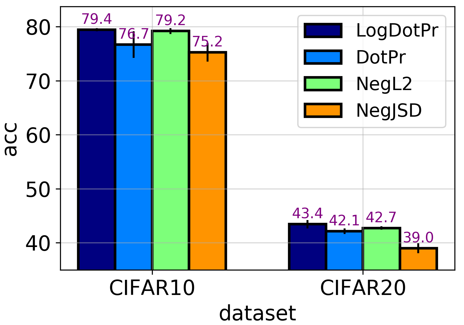
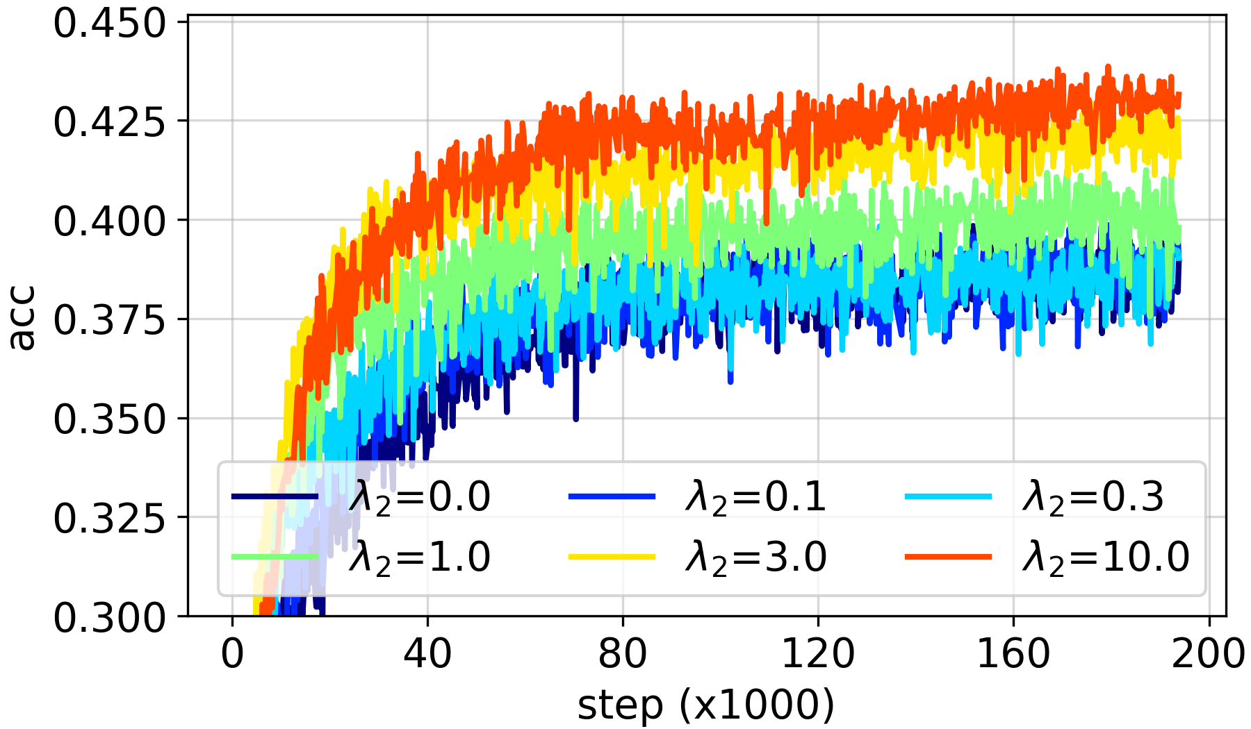
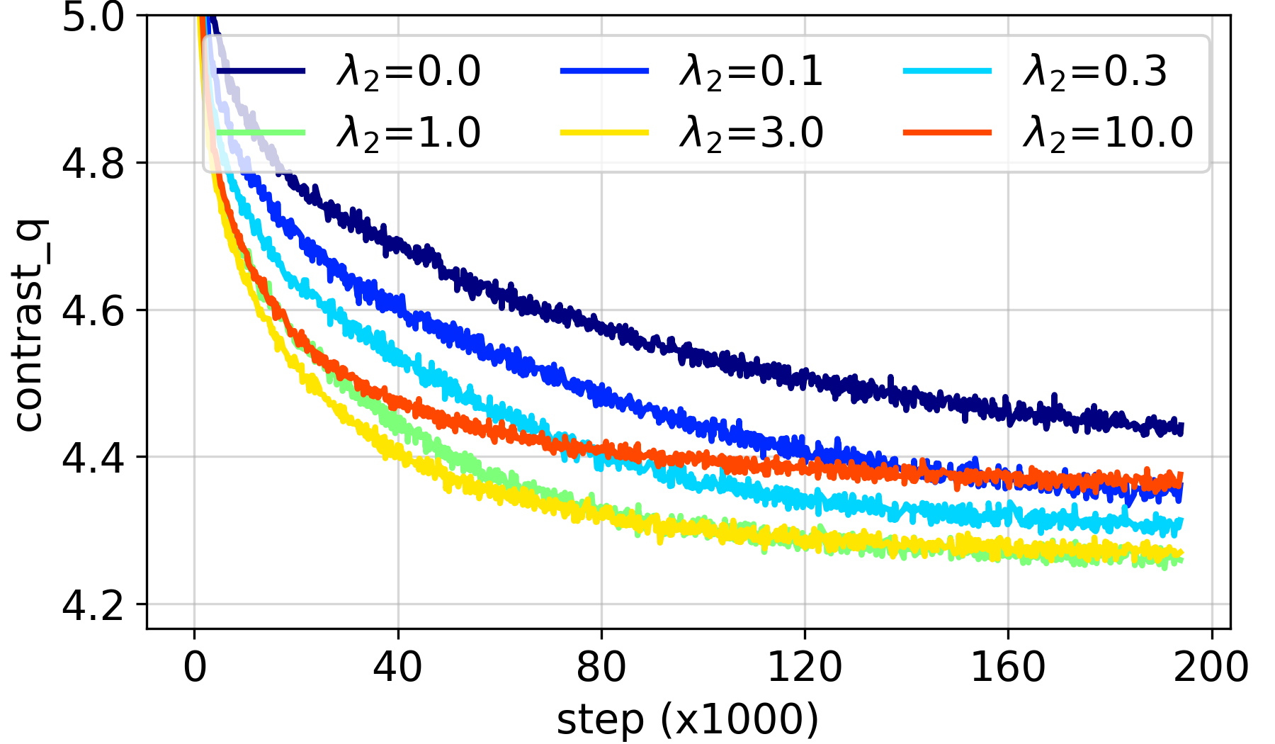
Figure 3: Left: Clustering accuracies of CRLC w.r.t. different critics on CIFAR10/20 (training set only). Middle, Right: Accuracy and $\mathcal{L}_{\text{PC}}$ curves of CRLC on CIFAR20 w.r.t. different coefficients of $\mathcal{L}_{\text{FC}}$ ($\lambda_{2}$ in Eq. 11).

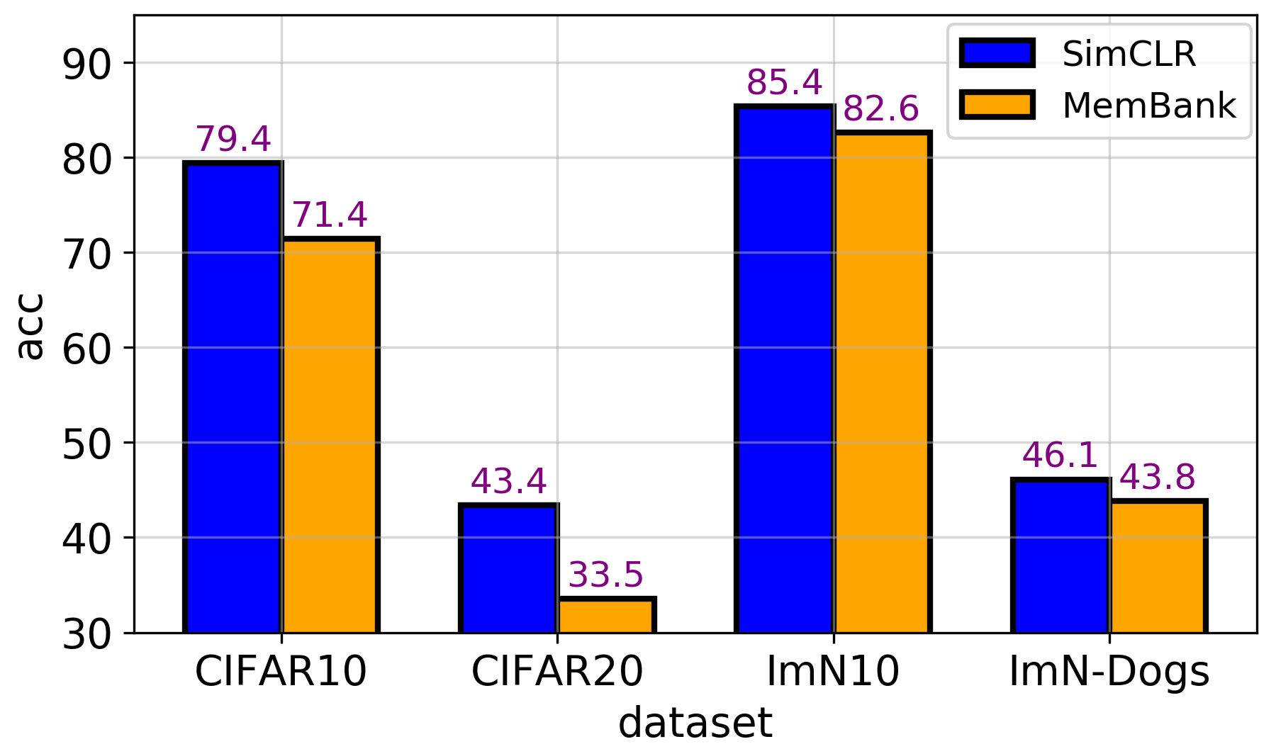
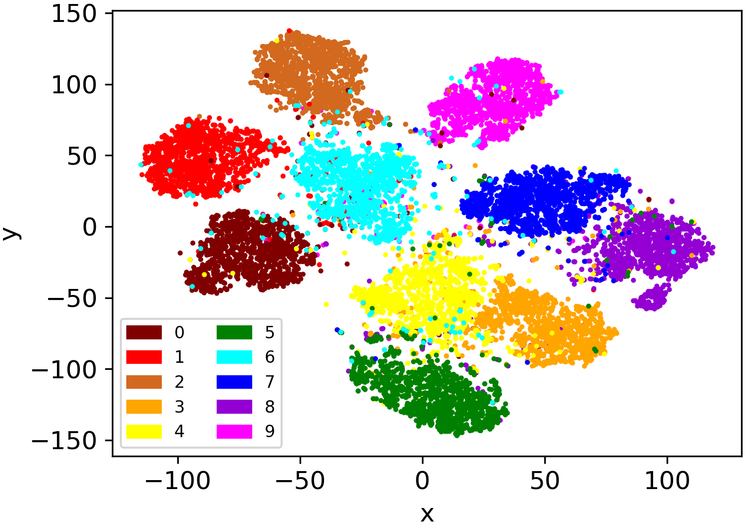
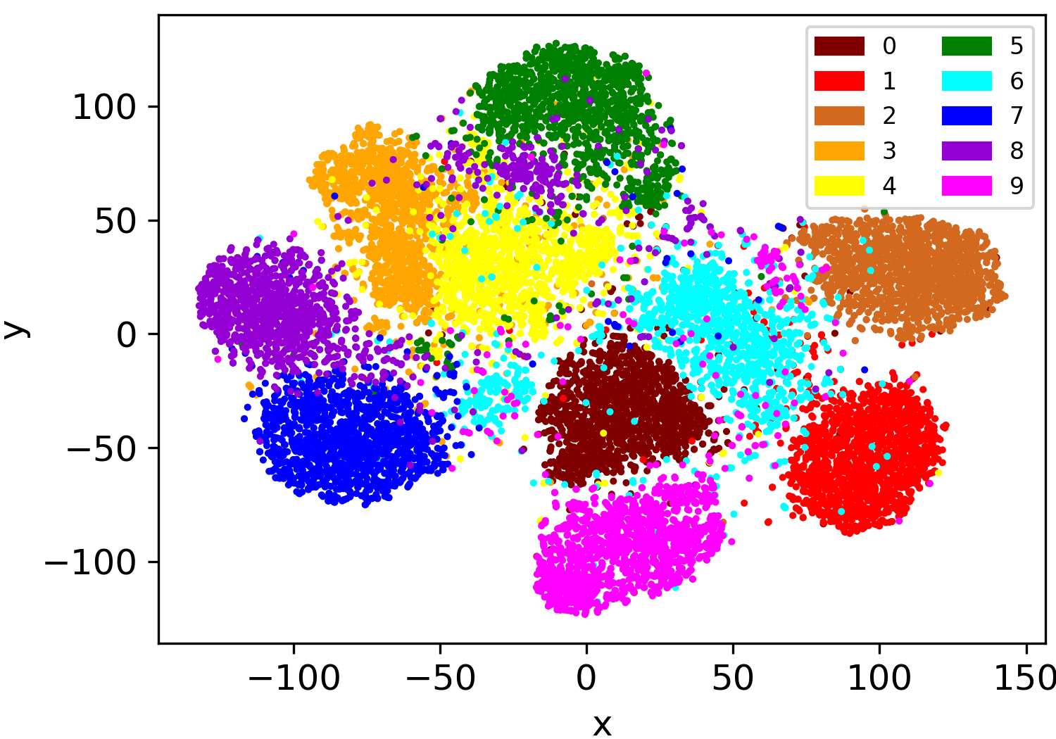
Figure 4: Left: Clustering accuracies of CRLC w.r.t. SimCLR [8] and MemoryBank [42] implementations. For CIFAR10/20, only the training set is used. Middle, Right: tSNE visualizations of the feature vectors learned by CRLC and SimCLR on the ImageNet10 train set, repectively.

From Table 3, we see that CRLC-semi, though is not designed especially for SSL, significantly outperforms many state-of-the-art SSL methods (brief discussion in Appdx. A.12). For example, CRLC-semi achieves about 30% and 10% lower error than MixMatch [3] and UDA [45] respectively on CIFAR10 with 4 labeled samples per class. Interestingly, the power of CRLC-semi becomes obvious when the number of labeled data is pushed to the limit. While most baselines cannot work with 1 or 2 labeled samples per class, CRLC-semi still performs consistently well with very low standard deviations. We hypothesize the reason is that CRLC-semi, via minimizing $\mathcal{L}_{\text{FC}}$, models the “smoothness” of data better than the SSL baselines. For more results on SSL, please check Appdx. A.14.

5.3 Ablation Study

Comparison of different critics in the probability contrastive loss

In Fig. 3 left, we show the performance of CRLC on CIFAR10 and CIFAR20 w.r.t. different critic functions. Apparently, the theoretically sound “log-of-dot-product” critic (Eq. 9) gives the best results. The “negative-L2-distance” critic is slightly worse than the “log-of-dot-product” critic while the “dot-product” and the “negative-JS-divergence” critics are the worst.

Contribution of the feature contrastive loss

We investigate by how much our model’s performance will be affected if we change the coefficient of $\mathcal{L}_{\text{FC}}$ ($\lambda_{2}$ in Eq. 11) to different values. Results on CIFAR20 are shown in Fig. 3 middle, right. Interestingly, minimizing both $\mathcal{L}_{\text{PC}}$ and $\mathcal{L}_{\text{FC}}$ simultaneously results in lower values of $\mathcal{L}_{\text{PC}}$ than minimizing only $\mathcal{L}_{\text{PC}}$ ($\lambda_{2}=0$). It implies that $\mathcal{L}_{\text{FC}}$ provides the model with more information to form better clusters. In order to achieve good clustering results, $\lambda_{2}$ should be large enough relative to the coefficient of $\mathcal{L}_{\text{PC}}$ which is 1. However, too large $\lambda_{2}$ results in a high value of $\mathcal{L}_{\text{PC}}$, which may hurts the model’s performance. For most datasets including CIFAR20, the optimal value of $\lambda_{2}$ is 10.

Nonparametric implementation of CRLC

Besides using SimCLR [8], we can also implement the two contrastive losses in CRLC using MemoryBank [42] (Section 3.1). This reduces the memory storage by about 30% and the training time by half (on CIFAR10 with ResNet34 as the backbone and the minibatch size of 512). However, MemoryBank-based CRLC usually takes longer time to converge and is poorer than the SimCRL-based counterpart as shown in Fig. 4 left. The contributions of the number of negative samples and the momentum coefficient to the performance of MemoryBank-based CRLC are analyzed in Appdx. A.10.2.

Mainfold visualization

We visualize the manifold of the continous features learned by CRLC in Fig. 4 middle. We observe that CRLC usually groups features into well-separate clusters. This is because the information captured by the C-head has affected the RL-head. However, if the RL-head is learned independently (e.g., in SimCLR), the clusters also emerge but are usually close together (Fig. 4 right). Through both cases, we see the importance of contrastive representation learning for clustering.

6 Conclusion

We proposed a novel clustering method named CRLC that exploits both the fine-grained instance-level information and the coarse-grained cluster-level information from data via a unified sample-oriented contrastive learning framework. CRLC showed promising results not only in clustering but also in semi-supervised learning. In the future, we plan to enhance CRLC so that it can handle neighboring samples in a principled way rather than just views. We also want to extend CRLC to other domains (e.g., videos, graphs) and problems (e.g., object detection).

Appendix A Appendix

A.1 Possible critics for the probability contrastive loss

We list here several possible critics that could be used in $\mathcal{L}_{\text{PC}}$. If we simply consider a critic $f$ as a similarity measure of two probabilities $p$ and $q$, $f$ could be the negative Jensen Shannon (JS) divergence between $p$ and $q$:

$$f(p,q) =-D_{\text{JS}}(p\|q)$$ (13)

$$=-\frac{1}{2}\left(D_{\text{KL}}\left(p\big{\|}\frac{p+q}{2}\right)+D_{\text{KL}}\left(q\big{\|}\frac{p+q}{2}\right)\right)$$ (14)

or the negative L2 distance between $p$ and $q$:

$$f(p,q)=-\left\|p-q\right\|_{2}^{2}=-\sum_{c=1}^{C}{(p_{c}-q_{c})}^{2}$$ (15)

In both cases, $f$ achieves its maximum value when $p=q$ and its minimum value when $p$ and $q$ are different one-hot vectors.

We can also define $f$ as the dot product of $p$ and $q$ as follows:

$$f(p,q)=p^{\top}q=\sum_{c=1}^{C}p_{c}q_{c}$$ (16)

However, the maximum value of this critic is no longer obtained when $p=q$ but when $p$ and $q$ are the same one-hot vector (check Appdx. A.2 for details). It means that maximizing this critic encourages not only the consistency between $p$ and $q$ but also the confidence of $p$ and $q$.

A.2 Global maxima and minima of the dot product critic for probabilities

(a) Dot-product critic

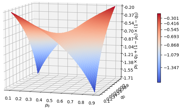
(b) Log-of-dot-product critic

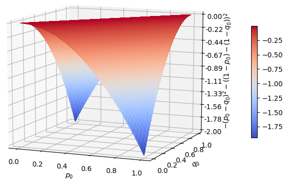
(c) Negative-L2-distance critic

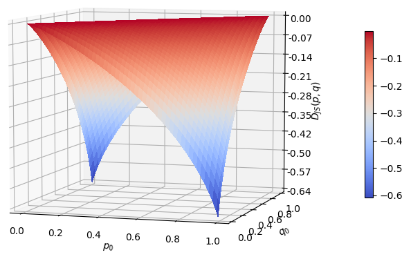
(d) Negative-JS-divergence critic

Figure 5: The surfaces of different critics on probabilities in case of 2 classes.

Proposition 1.

The dot product critic $f(p,q)=\sum_{c=1}^{C}p_{c}q_{c}$ achieves its global maximum value at $1$ when $p_{c}$ and $q_{c}$ are the same one-hot vector, and its global minimum value at $0$ when $p_{c}$ and $q_{c}$ are different one-hot vector.

Proof.

Since $0\leq p_{c},q_{c}\leq 1$, we have $\sum_{c=1}^{C}p_{c}q_{c}\geq 0$. This minimum value is achieved when $p_{c}q_{c}=0$ for all $c\in\{1,...,C\}$. And because $\sum_{c=1}^{C}p_{c}=\sum_{c=1}^{C}q_{c}=1$, $p_{c}$ and $q_{c}$ must be different one-hot vectors.

In addition, we also have $\sum_{c=1}^{C}p_{c}q_{c}\leq\sum_{c=1}^{C}p_{c}=1$. This maximum value is achieved when $p_{c}q_{c}=p_{c}$ or $p_{c}(q_{c}-1)=0$ for all $c\in\{1,...,C\}$, which means $p_{c}$ and $q_{c}$ must be the same one-hot vectors. ∎

Since the gradient of $\sum_{c=1}^{C}p_{c}q_{c}$ w.r.t. $q_{c}$ is proportional to $p_{c}$, if we fix $p$ and only optimize $q$, maximizing $\sum_{c=1}^{C}p_{c}q_{c}$ via gradient ascent will encourage $q$ to be one-hot at the component $k$ at which $p_{k}$ is the largest. Similarly, minimizing $\sum_{c=1}^{C}p_{c}q_{c}$ via gradient descent will encourage $q$ to be one-hot at the component $k$ at which $p_{k}$ is the smallest.

In case $p_{1}=...=p_{C}=\frac{1}{C}$, all the components of $q$ have similar gradients. Although it does not change the relative order between the components of $q$ after update, it still push $q$ towards the saddle point $\left(\frac{1}{C},...,\frac{1}{C}\right)$. However, chance that models get stuck at this saddle point is tiny unless we explicitly force it to happen (e.g., maximizing $H(q)$).

For better understanding of the optimization dynamics, we visualize the surface of $\sum_{c=1}^{C}p_{c}q_{c}$ with $C=2$ in Fig. 5a. $\log\left(\sum_{c=1}^{C}p_{c}q_{c}\right)$ has the same global optimal values and surface as $\sum_{c=1}^{C}p_{c}q_{c}$

A.3 Derivation of the InfoNCE lower bound

The variational lower bound of $I(X;Y)$ can be computed as follows:

$$I(X;Y) =\mathbb{E}_{p(x,y)}\left[\log\frac{p(x,y)}{p(x)p(y)}\right]$$

$$=\mathbb{E}_{p(x,y)}\left[\log\frac{q_{\theta}(x,y)}{p(x)p(y)}\right]+D_{\text{KL}}\left(p(x,y)\|q_{\theta}(x,y)\right)$$

$$\geq\mathbb{E}_{p(x,y)}\left[\log\frac{q_{\theta}(x,y)}{p(x)p(y)}\right]$$ (17)

where $q_{\theta}(x,y)$ is the variational approximation of $p(x,y)$.

Following [35], we assume that $q_{\theta}(x,y)$ belongs to the energy-based variational family that uses a critic $f_{\theta}(x,y)$ and is scaled by the data density $p(x)p(y)$:

$$q_{\theta}(x,y)=\frac{p(x)p(y)e^{f_{\theta}(x,y)}}{\sum_{x,y}p(x)p(y)e^{f_{\theta}(x,y)}}=\frac{p(x)p(y)e^{f_{\theta}(x,y)}}{Z_{\theta}}$$ (18)

where $Z_{\theta}=\sum_{x,y}p(x)p(y)e^{f_{\theta}(x,y)}=\mathbb{E}_{p(x)p(y)}\left[e^{f_{\theta}(x,y)}\right]$ is the partition function which does not depend on $x$, $y$.

Since the optimal value of $q_{\theta}(x,y)$ is $q_{\theta}^{*}(x,y)=p(x,y)$, we have:

$$\frac{p(x)p(y)e^{f_{\theta}^{*}(x,y)}}{Z_{\theta}^{*}}=p(x,y)$$

$$\Leftrightarrow f_{\theta}^{*}(x,y)=\log Z_{\theta}^{*}+\log\frac{p(x,y)}{p(x)p(y)},$$ (19)

which means the optimal value of $f_{\theta}(x,y)$ is proportional to $\log\frac{p(x,y)}{p(x)p(y)}$.

Next, we will show that $f_{\theta}$ is the critic in the InfoNCE lower bound. We start by rewriting the lower bound in Eq. 17 using the formula of $q_{\theta}(x)$ in Eq. 18 as follows:

$$I(X;Y) \geq\mathbb{E}_{p(x,y)}\left[\log\frac{e^{f_{\theta}(x,y)}}{Z_{\theta}}\right]$$

$$=\mathbb{E}_{p(x,y)}\left[f_{\theta}(x,y)\right]-\log Z_{\theta}$$ (20)

Here, we encounter the intractable $\log Z_{\theta}$. To form a tractable lower bound of $I(X;Y)$, we continue replacing $\log Z_{\theta}$ with its variational upper bound:

$$\log Z_{\theta}\leq\frac{Z_{\theta}}{a_{\theta}}+\log a_{\theta}-1$$ (21)

where $a_{\theta}$ is the variational approximation of $Z_{\theta}$. We should choose $a_{\theta}$ close to $Z_{\theta}$ so that the variance of the bound in Eq. 21 is small. Recalling that $Z_{\theta}=\mathbb{E}_{p(x)p(y)}\left[e^{f_{\theta}(x,y)}\right]$, we define $a_{\theta}$ as follows:

$$a_{\theta}=\frac{1}{M}\sum_{i=1}^{M}e^{f_{\theta}(x_{i},y)}$$ (22)

where $x_{1},...,x_{M}$ are $M$ samples from $p(x)$. $a_{\theta}$ in Eq. 22 can be seen as a stochastic estimation of $Z_{\theta}$ with $x$ sampled $M$ times more than $y$. Thus, $\frac{Z_{\theta}}{a_{\theta}}\approx 1$ and from Eq. 21, we have $\log Z_{\theta}\leq\log a_{\theta}$. Apply this result to Eq. 20, we have:

$$I(X;Y) \geq\mathbb{E}_{p(x,y)}\left[f_{\theta}(x,y)\right]-\log a_{\theta}$$ (23)

$$=\mathbb{E}_{p(x_{2:M})}\mathbb{E}_{p(x_{1},y)}\left[f_{\theta}(x_{1},y)-\log\frac{1}{M}\sum_{i=1}^{M}e^{f_{\theta}(x_{i},y)}\right]$$ (24)

$$=\mathbb{E}_{p(x_{1:M})p(y|x_{1})}\left[\log\frac{e^{f_{\theta}(x_{1},y)}}{\sum_{i=1}^{M}e^{f_{\theta}(x_{i},y)}}\right]+\log M$$ (25)

$$\triangleq I_{\text{InfoNCE}}(X;Y)$$ (26)

where Eq. 24 is obtained from Eq. 23 by using the fact that $\mathbb{E}_{p(x,y)}\left[f_{\theta}(x,y)\right]=\mathbb{E}_{p(x_{2:M})}\mathbb{E}_{p(x_{1},y)}\left[f_{\theta}(x_{1},y)\right]$ and the assumption that the samples $x_{1},...,x_{M}$ and $y$ in $a_{\theta}$ (Eq. 22) are drawn from $p(x_{2:M})p(x_{1},y)$.

Combining with the result in Eq. 19, we have the optimal critic $f_{\theta}^{*}(x,y)$ in the InfoNCE lower bound is proportional to $\log\frac{p(x,y)}{p(x)p(y)}=\log\frac{p(y|x)}{p(y)}$. Since $p(y)$ does not depend on $x$ and will be cancelled by both the nominator and denominator in Eq. 25, $f_{\theta}^{*}(x,y)$ is, in fact, proportional to $\log p(y|x)$.

A.4 Derivation of the scaled dot product critic in representation learning

Recalling that in contrastive representation learning, the critic $f$ is defined as the scaled dot product between two unit-normed feature vectors $\tilde{z}$, $z_{i}$:

$$f(\tilde{x},x_{i})=\tilde{z}^{\top}z_{i}/\tau$$

Interestingly, this formula of $f$ is accordant with the formula of $f^{*}$ and is proportional to $\log p(\tilde{x}|x_{i})$. To see why, let’s assume that the distribution of $\tilde{z}$ given $z_{i}$ is modeled by an isotropic Gaussian distribution with $z_{i}$ as the mean vector and $\tau I$ as the covariance matrix. Then, we have:

$$f^{*} \propto\log p(\tilde{x}|x_{i})$$

$$\approx\log p(\tilde{z}|z_{i})$$

$$\propto\log e^{-\frac{0.5}{\tau}\left\|\tilde{z}-z_{i}\right\|_{2}^{2}}$$

$$=-\frac{0.5}{\tau}\left(\left\|\tilde{z}\right\|_{2}^{2}-2\tilde{z}^{\top}z_{i}+\left\|z_{i}\right\|_{2}^{2}\right)$$

$$=\tilde{z}^{\top}z_{i}/\tau-1/\tau$$

$$\propto\tilde{z}^{\top}z_{i}/\tau$$

where $\left\|\tilde{z}\right\|_{2}^{2}=\left\|z_{i}\right\|_{2}^{2}=1$ due to the fact that $\tilde{z}$ and $z_{i}$ are unit-normed vectors.

A.5 Analysis of the gradient of $\mathcal{L}_{\text{PC}}$

Recalling that the probability contrastive loss $\mathcal{L}_{\text{PC}}$ for a sample $\tilde{x}$ with the “log-of-dot-product” critic $f(p,q)=\log\left(p^{\top}q\right)$ is computed as follows:

$$\mathcal{L}_{\text{PC}} =-\log\frac{e^{f(\tilde{q},q_{1})}}{\sum_{i=1}^{M}e^{f(\tilde{q},q_{i})}}$$

$$=-\log\left(\tilde{q}^{\top}q_{1}\right)+\log\sum_{i=1}^{M}\tilde{q}^{\top}q_{i}$$

Because $\tilde{q}$ is always parametric while $q_{i}$ ($i\in\{1,...,M\}$) can be either parametric (if $\mathcal{L}_{\text{PC}}$ is implemented via the SimCLR framework [8]) or non-parametric (if $\mathcal{L}_{\text{PC}}$ is implemented via the MemoryBank framework [42]), we focus on the gradient of $\mathcal{L}_{\text{PC}}$ back-propagating through $\tilde{q}$. In practice, $\tilde{q}$ is usually implemented by applying softmax to the logit vector $\tilde{u}\in\mathbb{R}^{C}$:

$$\tilde{q}_{c}=\frac{\exp\left(\tilde{u}_{c}\right)}{\sum_{k=1}^{C}\exp\left(\tilde{u}_{k}\right)}$$

where $\tilde{q}_{c}$ denotes the $c$-th component of $\tilde{q}$. Similarly, $q_{i,c}$ is the $c$-th component of $q_{i}$.

The gradient of $\mathcal{L}_{\text{PC}}$ w.r.t. $\tilde{u}_{c}$ is given by:

$$\frac{\partial\mathcal{L}_{\text{PC}}}{\partial\tilde{u}_{c}}=-\frac{\partial}{\partial\tilde{u}_{c}}\log\left(\tilde{q}^{\top}q_{1}\right)+\frac{\partial}{\partial\tilde{u}_{c}}\log\sum_{i=1}^{M}\tilde{q}^{\top}q_{i}$$ (27)

The first term in Eq. 27 is equivalent to:

$$-\frac{\partial}{\partial\tilde{u}_{c}}\log\left(\tilde{q}^{\top}q_{1}\right)$$

$$\Leftrightarrow \frac{-1}{\tilde{q}^{\top}q_{1}}\left(\frac{\partial}{\partial\tilde{u}_{c}}\left(\tilde{q}_{c}q_{1,c}\right)+\sum_{k\neq c}\frac{\partial}{\partial\tilde{u}_{c}}\left(\tilde{q}_{k}q_{1,k}\right)\right)$$

$$\Leftrightarrow \frac{-1}{\tilde{q}^{\top}q_{1}}\left(\tilde{q}_{c}(1-\tilde{q}_{c})q_{1,c}-\sum_{k\neq c}\tilde{q}_{c}\tilde{q}_{k}q_{1,k}\right)$$

$$\Leftrightarrow -\frac{1}{\sum_{k=1}^{C}\tilde{q}_{k}q_{1,k}}\left(\tilde{q}_{c}q_{1,c}-\tilde{q}_{c}\sum_{k=1}^{C}\tilde{q}_{k}q_{1,k}\right)$$

$$\Leftrightarrow \tilde{q}_{c}-\frac{\tilde{q}_{c}q_{1,c}}{\sum_{k=1}^{C}\tilde{q}_{k}q_{1,k}}$$ (28)

And the second term in Eq. 27 is equivalent to:

$$\frac{\partial}{\partial\tilde{u}_{c}}\log\sum_{i=1}^{M}\tilde{q}^{\top}q_{i}$$

$$\Leftrightarrow \frac{1}{\sum_{i=1}^{M}\tilde{q}^{\top}q_{i}}\left(\sum_{i=1}^{M}\frac{\partial}{\partial\tilde{u}_{c}}\left(\tilde{q}^{\top}q_{i}\right)\right)$$

$$\Leftrightarrow \frac{1}{\sum_{i=1}^{M}\tilde{q}^{\top}q_{i}}\left(\sum_{i=1}^{M}\left(\tilde{q}_{c}q_{i,c}-\tilde{q}_{c}\sum_{k=1}^{C}\tilde{q}_{k}q_{i,k}\right)\right)$$

$$\Leftrightarrow \frac{1}{\sum_{i=1}^{M}\sum_{k=1}^{C}\tilde{q}_{k}q_{i,k}}\left(\sum_{i=1}^{M}\tilde{q}_{c}q_{i,c}-\tilde{q}_{c}\sum_{i=1}^{M}\sum_{k=1}^{C}\tilde{q}_{k}q_{i,k}\right)$$

$$\Leftrightarrow \frac{\sum_{i=1}^{M}\tilde{q}_{c}q_{i,c}}{\sum_{i=1}^{M}\sum_{k=1}^{C}\tilde{q}_{k}q_{i,k}}-\tilde{q}_{c}$$

Thus, we have:

$$\frac{\partial\mathcal{L}_{\text{PC}}}{\partial\tilde{u}_{c}}=\frac{\sum_{i=1}^{M}\tilde{q}_{c}q_{i,c}}{\sum_{i=1}^{M}\sum_{k=1}^{C}\tilde{q}_{k}q_{i,k}}-\frac{\tilde{q}_{c}q_{1,c}}{\sum_{k=1}^{C}\tilde{q}_{k}q_{1,k}}$$ (29)

We care about the second term in Eq. 29 which is derived from the gradient of the critic $f(\tilde{q},q_{1})$ w.r.t. $\tilde{u}_{c}$ (the negative of the term in Eq. 28). We rewrite this gradient with simplified notations as follows:

$$\frac{\partial f(q,p)}{\partial u_{c}}=\frac{q_{c}p_{c}}{\sum_{k=1}^{C}q_{k}p_{k}}-q_{c}$$

where $u_{c}$ is the $c$-th logit of $q$. Since during training, $q$ is encouraged to be one-hot (see Appdx. A.2), the denominator may not be defined if we do not prevent $p$ from being a different one-hot vector. However, even when the denominator is defined, the update still does not happen as expected when $q$ is one-hot. To see why, let’s consider a simple scenario in which $q=[0,1,0]$ and $p=[0.998,0.001,0.001]$. Apparently, the denominator is 0.001 $\neq$ 0. By maximizing $f(q,p)$, we want to push $q$ toward $p$. Thus, we expect that $\frac{\partial f}{\partial u_{1}}>0$ and $\frac{\partial f}{\partial u_{2}}<0$. However, the gradients w.r.t. $u_{c}$ are 0s for all $c\in\{1,2,3\}$:

$$\frac{\partial f}{\partial u_{1}} =\frac{0\times 0.998}{0.001}-0=0$$

$$\frac{\partial f}{\partial u_{2}} =\frac{1\times 0.001}{0.001}-1=0$$

$$\frac{\partial f}{\partial u_{3}} =\frac{0\times 0.001}{0.001}-0=0$$

The reason is that $q=[0,1,0]$ is a stationary point (minimum in this case). This means once the model has set $q$ to be one-hot, it tends to get stuck there and cannot escape regardless of the value of $p$. This problem is known in literature as the “saturating gradient” problem. To alleviate this problem, we propose to smooth out the values of $q$ and $p$ before computing the critic $f$:

$$q =(1-\gamma)q+\gamma r$$

$$p =(1-\gamma)p+\gamma r$$

where $0\leq\gamma\leq 1$ is the smoothing coefficient, which is set to 0.01 if not otherwise specified; $r=\left(\frac{1}{C},...,\frac{1}{C}\right)$ is the uniform probability vector over classes. We also regularize the value of $u_{c}$ to be within $[-25,25]$.

Dataset	#Train	#Test	#Extra	#Classes	Image size
CIFAR10	50,000	10,000	$\times$	10	32$\times$32$\times$3
CIFAR20	50,000	10,000	$\times$	20	32$\times$32$\times$3
STL10	5,000	8,000	100,000	10	96$\times$96$\times$3
ImageNet10	13,000	500	$\times$	10	224$\times$224$\times$3
ImageNet-Dogs	19,500	750	$\times$	15	224$\times$224$\times$3
ImageNet-50	64,274	2,500	$\times$	50	224$\times$224$\times$3
ImageNet-100	128,545	5,000	$\times$	100	224$\times$224$\times$3
ImageNet-200	256,558	10,000	$\times$	200	224$\times$224$\times$3

Table 4: Details of the datasets used in this work.

Dataset		CIFAR10			CIFAR20			STL10
Metric		ACC	NMI	ARI	ACC	NMI	ARI	ACC	NMI	ARI
C-head only	Train only	67.2$\pm$0.7	56.8$\pm$1.3	47.8$\pm$1.4	38.0$\pm$1.6	36.8$\pm$1.0	22.3$\pm$0.9	47.03$\pm$2.2	39.06$\pm$1.5	27.23$\pm$1.8
	Train + Test	66.9$\pm$0.8	56.9$\pm$0.7	47.5$\pm$0.5	37.7$\pm$0.4	35.7$\pm$0.5	21.6$\pm$0.3	61.2$\pm$1.2	52.7$\pm$0.8	43.4$\pm$1.3
CRLC	Train only	79.4$\pm$0.3	66.7$\pm$0.6	62.3$\pm$0.4	43.4$\pm$0.8	43.1$\pm$0.5	27.7$\pm$0.3	57.6$\pm$1.6	50.8$\pm$1.5	41.9$\pm$1.2
	Train + Test	79.9$\pm$0.6	67.9$\pm$0.6	63.4$\pm$0.4	42.5$\pm$0.7	41.6$\pm$0.8	26.3$\pm$0.5	81.8$\pm$0.3	72.9$\pm$0.4	68.2$\pm$0.3

Table 5: Clustering results of our proposed methods on CIFAR10, CIFAR20 and STL10 with only the training set used and with both the training and test sets used.

Dataset	ImageNet10			ImageNet-Dogs
Metric	ACC	NMI	ARI	ACC	NMI	ARI
C-head only	80.0$\pm$1.4	75.2$\pm$1.9	67.6$\pm$2.2	36.3$\pm$0.9	37.5$\pm$0.7	19.8$\pm$0.4
CRLC	85.4$\pm$0.3	83.1$\pm$0.5	75.9$\pm$0.4	46.1$\pm$0.6	48.4$\pm$0.6	29.7$\pm$0.4

Table 6: Clustering results of our proposed methods on ImageNet10 and ImageNet-Dogs.

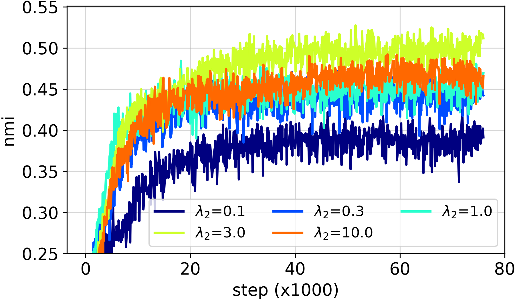
Figure 6: NMI curve of CRLC on ImageNet-Dogs w.r.t. different coefficients of $\mathcal{L}_{\text{FC}}$.

A.6 Dataset description

In Table 4, we provide details of the datasets used in this work. CIFAR20 is CIFAR100 with 100 classes replaced by 20 super-classes. STL10 is different from other datasets in the sense that it has an auxiliary set of 100,000 unlabeled samples of unknown classes. Similar to previous works, we use samples from this auxiliary set and the training set to train the “representation learning” head.

A.7 Training setups for clustering

End-to-end clustering

For end-to-end clustering, we use a SGD optimizer with a constant learning rate = 0.1, momentum = 0.9, Nesterov = False, and weight decay = 5e-4 based on the settings in [13, 16, 39]. We set the batch size to 512 and the number of epochs to 2000. In fact, on some datasets like ImageNet10 or ImageNet-Dogs, CRLC only needs 500 epochs to converge. The coefficients of the negative entropy and $\mathcal{L}_{\text{FC}}$ ($\lambda_{1}$ and $\lambda_{2}$ in Eq. 11 in the main text) are fixed at 1 and 10, respectively. Each experiment is repeated 3 times with random initializations.

Two-stage clustering

For two-stage clustering, we use the same settings as in [40]. Specifically, the backbone network is ResNet18 for CIFAR10/20, STL10 and is ResNet50 for ImageNet50/100/200. In the first (pretraining) stage, for CIFAR10/20 and STL10, we pretrain the backbone network and the RL-head via SimCLR [8] for 500 epochs. The optimizer is SGD with an initial learning rate = 0.4 decayed with a cosine decay schedule [28], momentum = 0.9, Nesterov = False, and weight decay = 1e-4. Meanwhile, for ImageNet50/100/200, we directly copy the pretrained weights of MoCo [16] to the backbone network and the RL-head. After the pretraining stage, we find for each sample in the training set 50 nearest neighbors based on the cosine similarity measure. Positive samples for contrative learning in the second stage are drawn uniformly from these sets of nearest neighbors. In the second stage, for CIFAR10/20 and STL10, we train both the backbone network and the C-head for 200 epochs by minimizing $\mathcal{L}_{\text{cluster}}$ (Eq. 8 in the main text) using an Adam optimizer with a constant learning rate = 1e-4 and weight decay = 1e-4. For ImageNet50/100/200, we freeze the backbone network and only train the C-head for 200 epochs by minimizing $\mathcal{L}_{\text{cluster}}$ using an SGD optimizer with a constant learning rate = 5.0, momentum = 0.9, Nesterov = False, and weight decay = 0.0.

Dataset	CIFAR10			CIFAR20			STL10
Metric	ACC	NMI	ARI	ACC	NMI	ARI	ACC	NMI	ARI
K-means [40]	65.9$\pm$5.7	59.8$\pm$2.0	50.9$\pm$3.7	39.5$\pm$1.9	40.2$\pm$1.1	23.9$\pm$1.1	65.8$\pm$5.1	60.4$\pm$2.5	50.6$\pm$4.1
SCAN [40]	81.8$\pm$0.3	71.2$\pm$0.4	66.5$\pm$0.4	42.2$\pm$3.0	44.1$\pm$1.0	26.7$\pm$1.3	75.5$\pm$2.0	65.4$\pm$1.2	59.0$\pm$1.6
two-stage CRLC	84.2$\pm$0.1	74.7$\pm$0.3	70.6$\pm$0.5	45.0$\pm$0.7	44.8$\pm$0.8	28.7$\pm$0.9	78.7$\pm$1.1	68.4$\pm$1.6	62.7$\pm$1.8

Table 7: Two-stage clustering results on CIFAR10/20 and STL10.

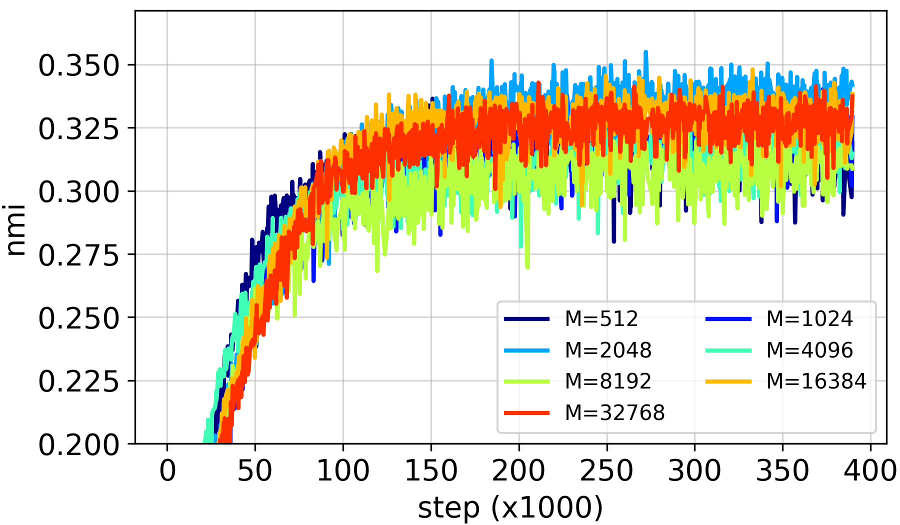
(a) NMI

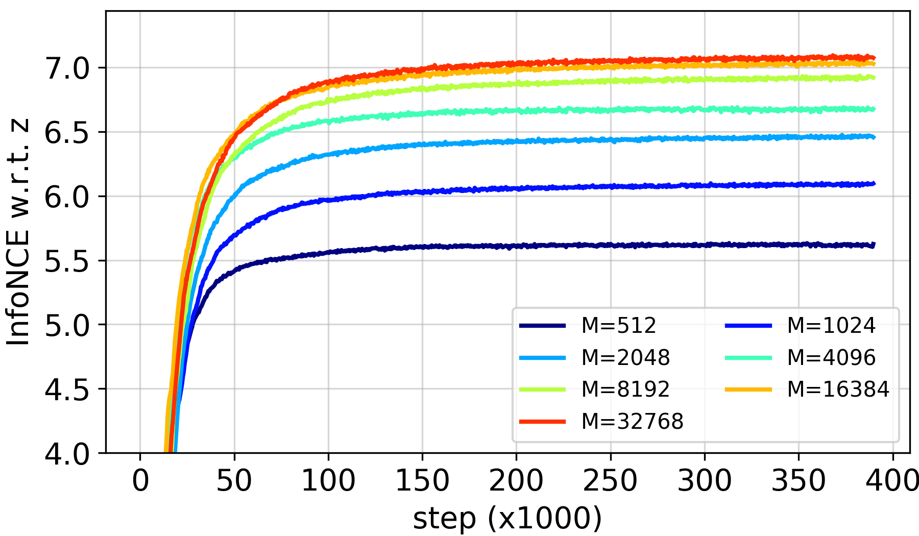
(b) InfoNCE w.r.t. $\mathcal{L}_{\text{FC}}$

(c) InfoNCE w.r.t. $\mathcal{L}_{\text{PC}}$

Figure 7: Learning curves of MemoryBank-based CRLC on CIFAR20 w.r.t. different numbers of negative samples. The momentum is $\alpha=0.5$. The InfoNCE w.r.t. a contrastive loss is computed by using Eq. 2 in the main text.

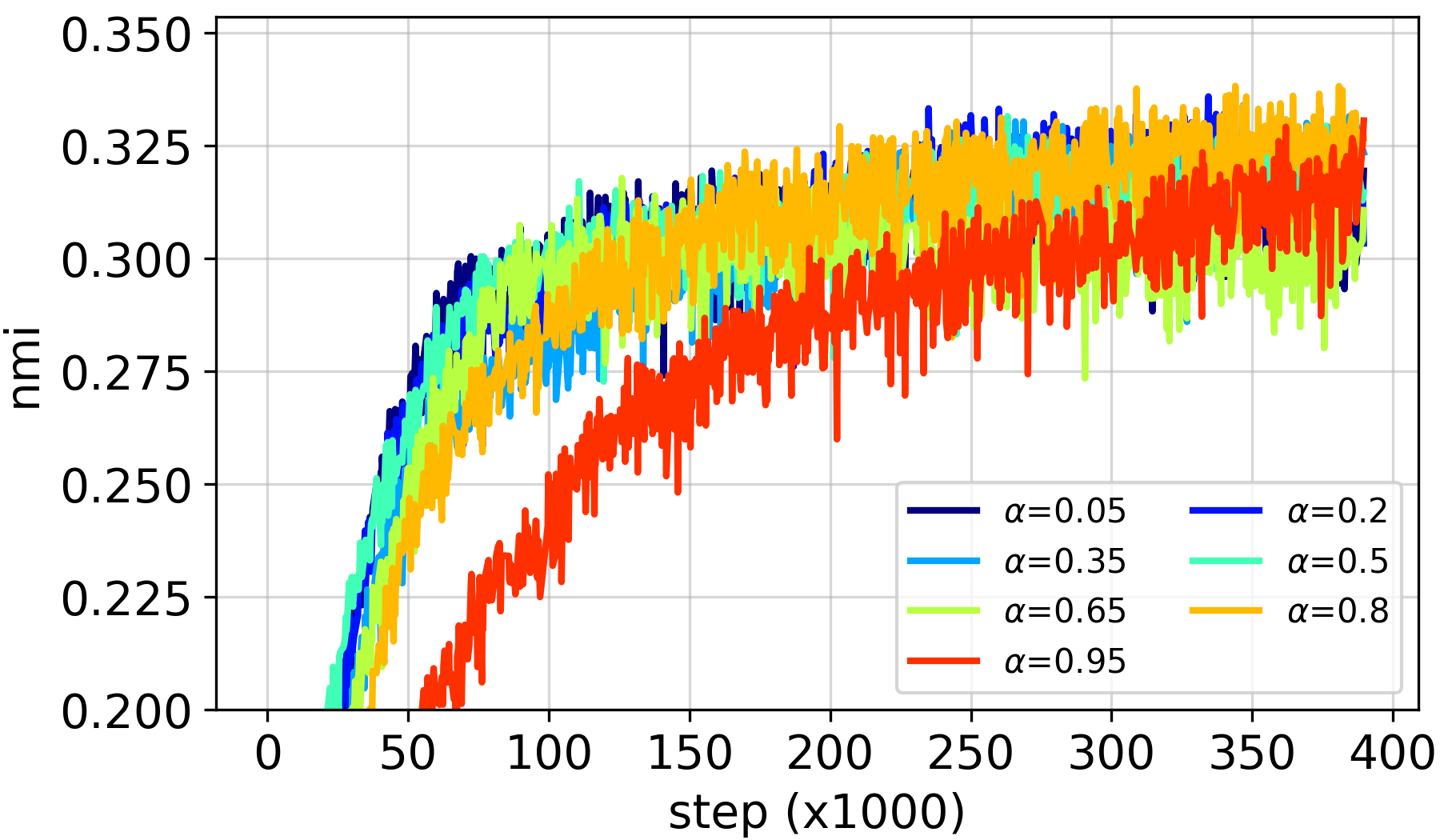
(a) NMI

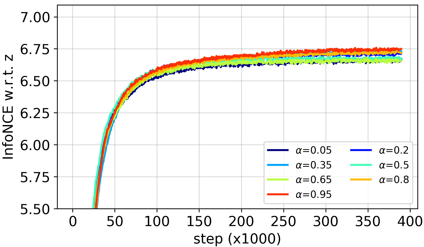
(b) InfoNCE w.r.t. $\mathcal{L}_{\text{FC}}$

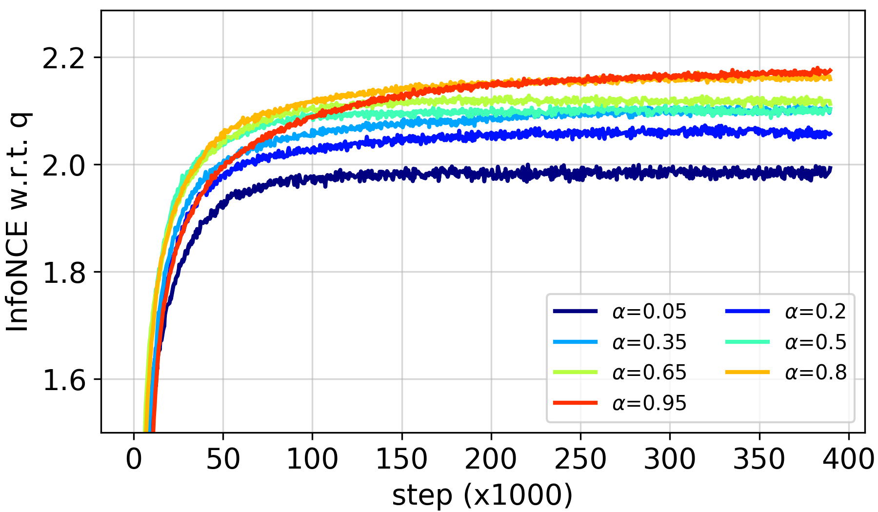
(c) InfoNCE w.r.t. $\mathcal{L}_{\text{PC}}$

Figure 8: Learning curves of MemoryBank-based CRLC on CIFAR20 w.r.t. different values of the momentum. The number of negative samples is $M=4096$. The InfoNCE w.r.t. a contrastive loss is computed by using Eq. 2 in the main text.

A.8 Complete end-to-end clustering results

Complete results with standard deviations on the five standard clustering datasets are shown in Tables 5 and 6. From Table 5, we see that for CIFAR10 using both the training and test sets does not cause much difference in performance compared to using only the training set. For CIFAR20, using only the training set even leads to slightly better results. By contrast, for STL10, models trained with both the training and test sets significantly outperform those trained with the training set only. We believe the reason is that for CIFAR10 and CIFAR20, the training set is big enough to cover the data distribution in the test set while for STL10, it does not apply (Table 4). Therefore, we think subsequent works should use only the training set when doing experiments on CIFAR10 and CIFAR20.

A.9 Additional two-stage clustering results

Table 7 compares the clustering results of “two-stage” CRLC and SCAN on CIFAR10/20, STL10. “Two-stage” CRLC clearly outperforms SCAN on all datasets.

A.10 Additional ablation study results

A.10.1 Contribution of the feature contrastive loss

In Fig. 6, we show the performance of CRLC on ImageNet-Dogs w.r.t. different coefficients of $\mathcal{L}_{\text{FC}}$ ($\lambda_{2}$ in Eq. 11 in the main text). We observe that CRLC achieves the best clustering accuracy when $\lambda_{2}=3$. However, in Table 1 in the main text, we still report the result when $\lambda_{2}=10$.

A.10.2 Nonparametric implementation of CRLC

In this section, we empirically investigate the contributions of the number of negative samples and the momentum coefficient ($\alpha$ in Eq. 10 in the main text) to the performance of MemoryBank-based CRLC.

Contribution of the number of negative samples

From Fig. 7a, we do not see any correlation between the number of negative samples and the clustering performance of MemoryBank-baed CRLC despite the fact that increasing the number of negative samples allows the RL-head and the C-head to gain more information from data (Figs. 7b and 7c). It suggests that for clustering (and possibly other classification tasks), getting more information may not lead to good results. Instead, we need to extract the right information related to clusters.

Contribution of the momentum coefficient

From Fig. 8b, we see that changing the momentum value for updating probability vectors stored in the memory bank does not affects amount of information captured by the RL-head much. By contrast, in Fig. 8c, we see that larger values of the momentum cause the C-head to capture more information. This is reasonable because the accumulated probability vector $q_{n,t}$ is usually more stochastic (contains more information) than the probability vector $\hat{q}_{n}$ of a particular view (Eq. 10 in the main text). Larger values of the momentum also cause the model to converge slower but do not affect the performance much (Fig. 8a).

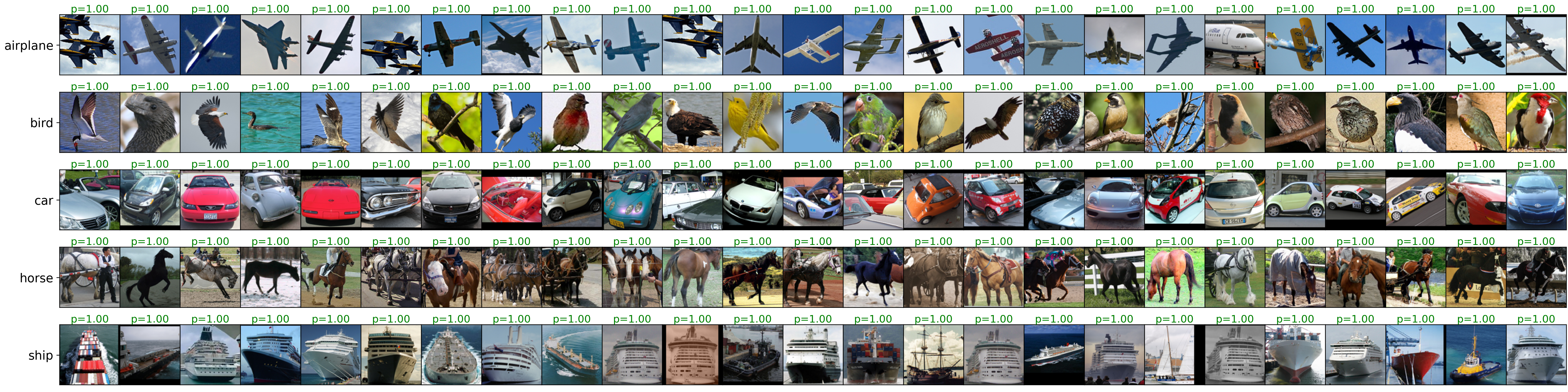
Figure 9: STL10 samples of 5 classes correctly predicted by CRLC. Samples are sorted by their confidence scores.

A.11 Qualitative evaluation

In Fig. 9, we show the top correctly predicted samples according to their confidence score for each of 5 classes from the training set of STL10. It is clear that these samples are representative of the cluster they belong to.

A.12 Consistency-regularization-based semi-supervised learning methods

When some labeled data are given, the clustering problem naturally becomes semi-supervised learning (SSL). The core idea behind recent state-of-the-art SSL methods such as UDA [45], MixMatch [3], ReMixMatch [2], FixMatch [36] is consistency regularization (CR) which is about forcing an input sample under different perturbations/augmentations to have similar class predictions. In this sense, CR can be seen as an unnormalized version of the probability contrastive loss without the denominator. Different SSL methods extend CR in different ways. For example, UDA uses strong data augmentation to generate positive pairs. MixMatch and ReMixMatch combines CR with MixUp [52]. However, none of the above methods achieve consistent performance with extremely few labeled data (Section 5.2 in the main text). By contrast, clustering methods like CRLC perform consistently well even when no label is available. Thus, we believe designing a method that enjoys the strength of both fields is possible and CRLC-semi can be one step towards that goal.

A.13 Training setups for semi-supervised learning

To train CRLC-semi, we use a SGD optimizer with an initial learning rate = 0.1, momentum = 0.9, Nesterov = False, and weight decay = 5e-4. Similar to [36], we adjust the learning rate at each epoch using a cosine decay schedule [28] computed as follows:

$$\text{lr}_{t}=\text{\text{lr}}_{\text{min}}+(\text{lr}_{\text{init}}-\text{lr}_{\text{min}})\times\frac{1+\cos\left(\frac{t}{T}\pi\right)}{2}$$

where $\text{lr}_{\text{init}}=0.1$, $\text{lr}_{\text{min}}=0.001$, $\text{lr}_{t}$ is the learning rate at epoch $t$ over $T$ epochs in total. $T$ is 2000 and 1000 for CIFAR10 and CIFAR100, respectively. The number of labeled and unlabeled samples in each batch is 64 and 512, respectively. In $\mathcal{L}_{\text{CRLC-semi}}$ (Eq. 12 in the main text), $\lambda_{1}=1$, $\lambda_{2}=5$, and $\lambda_{3}=1$.

We reimplement FixMatch using sample code from Github with the default settings unchanged. In this code, the number of labeled and unlabeled data in a batch is 64 and 448, respectively. However, the number of steps in one epoch does not depend on the batch size but is fixed at 1024. Thus, FixMatch is trained in 1024 epochs $\approx$ 1 million steps for both CIFAR10 and CIFAR100. Meanwhile, CLRC-semi is trained in only 194,000 steps for CIFAR10 and 97,000 steps for CIFAR100.

Dataset	CIFAR10				CIFAR100
Labels	10	20	40	250	100	200	400	2500
$\Pi$-model [24]	-	-	-	54.26$\pm$3.97	-	-	-	57.25$\pm$0.48
Pseudo Labeling [25]	-	-	-	49.78$\pm$0.43	-	-	-	57.38$\pm$0.46
Mean Teacher [38]	-	-	-	32.32$\pm$2.30	-	-	-	53.91$\pm$0.57
MixMatch [3]	-	-	47.54$\pm$11.50	11.05$\pm$0.86	-	-	67.61$\pm$1.32	39.94$\pm$0.37
UDA [45]	-	-	29.05$\pm$5.93	8.82$\pm$1.08	-	-	59.28$\pm$0.88	33.13$\pm$0.22
ReMixMatch [2]	-	-	19.10$\pm$9.64	5.44$\pm$0.05	-	-	44.28$\pm$2.06	27.43$\pm$0.31
FixMatch (RA) [36]	-	-	13.81$\pm$3.37	5.07$\pm$0.65	-	-	48.85$\pm$1.75	28.29$\pm$0.11
ReMixMatch†	59.86$\pm$9.34	41.68$\pm$8.15	28.31$\pm$6.72	-	76.32$\pm$4.30	66.51$\pm$2.86	52.23$\pm$1.71	-
FixMatch (RA)†	25.49$\pm$7.74	21.15$\pm$8.96	8.87$\pm$4.29	-	79.27$\pm$2.65	68.58$\pm$0.7	57.52$\pm$1.5	-
CRLC-semi	46.75$\pm$8.01	29.81$\pm$1.18	19.87$\pm$0.82	13.53$\pm$0.21	82.20$\pm$1.15	73.04$\pm$1.15	60.87$\pm$0.17	41.10$\pm$0.12

Table 8: Full classification errors on CIFAR10 and CIFAR100. Lower values are better. Results of baselines are taken from [36]. ^†: Results obtained from external implementations of models.

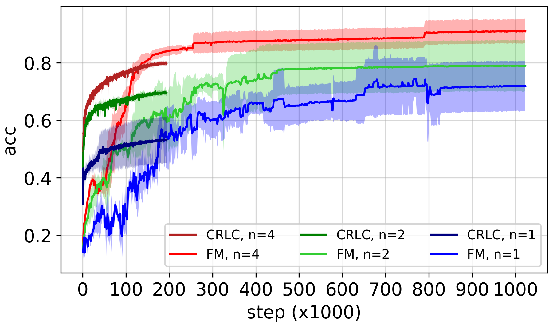
(a) CIFAR10

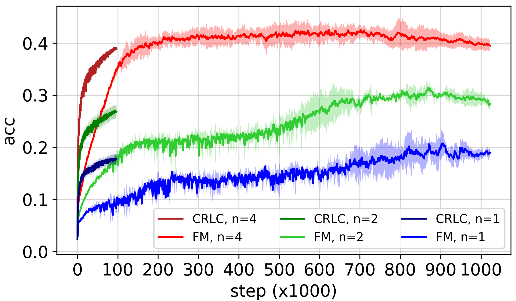
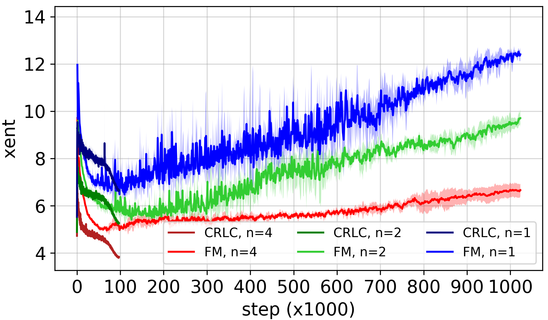
(b) CIFAR100

Figure 10: Test accuracy and crossentropy curves of CRLC-semi (CRLC) and FixMatch (FM) on CIFAR10 and CIFAR100 with 1, 2, 4 labeled samples per class. It is clear that CRLC-semi performs consistently in all cases except for the case of CIFAR10 with 1 labeled sample per class. However, even in that case, the CRLC-semi still gives consistent performance for each run (Fig. 11). FixMatch, by contrast, is very inconsistent in its performance for each run, especially on CIFAR10.

A.14 More results on semi-supervised learning

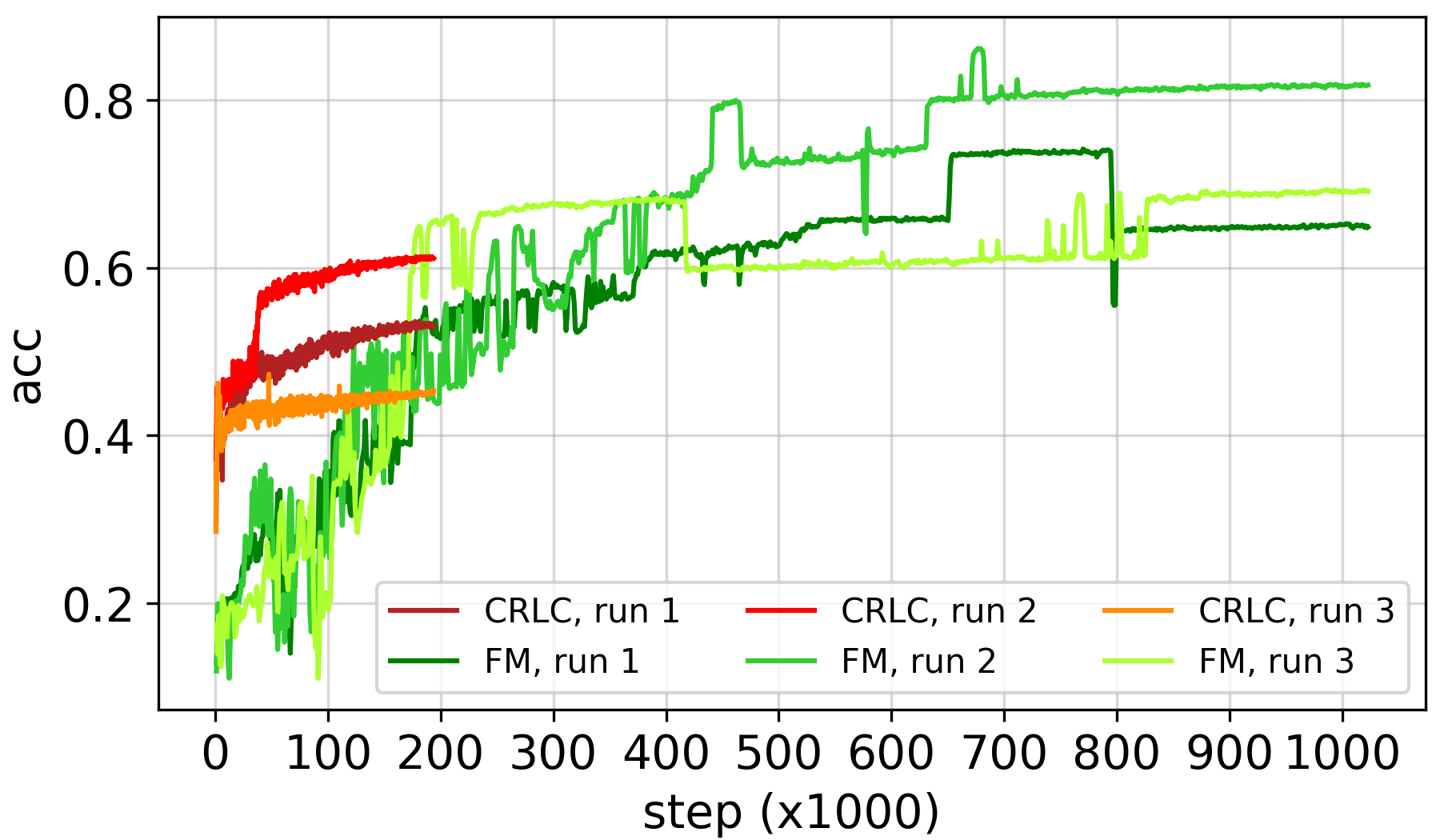
Figure 11: Test accuracy curves of CRLC-semi (CRLC) and FixMatch (FM) on CIFAR10 with 1 labeled samples per class w.r.t. 3 different runs.

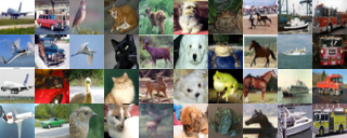
Figure 12: 40 labeled CIFAR10 samples organized into 4 rows where each row has 10 images corresponding to 10 classes. For 10 and 20 labeled samples, the first row and the first two rows are considered, respectively.

Figure 13: Indices in the training set of the images in Fig. 12

In Table 8, we show additional semi-supervised learning results of CRLC-semi on CIFAR10 and CIFAR100 in comparison with more baselines. CRLC-semi clearly outperforms all standard baselines like $\Pi$-model, Pseudo Labeling or Mean Teacher. However, CRLC-semi looses its advantage over holistic methods like MixMatch [3] and methods that use strong data augmentation like UDA [45] or ReMixMatch [2] when the number of labeled data is big enough. Currently, we are not sure whether the problem comes from the feature contrastive loss $\mathcal{L}_{\text{FC}}$ (when we have enough labels, representation learning may act as a regularization term and reduce the classification result), or from the negative entropy term in $\mathcal{L}_{\text{cluster}}$ (causing too much regularization), or even from the probability contrastive loss (contrasting probabilities of two related views is not suitable when we have enough labels). Thus, we leave the answer of this question for future work. To gain more insight about the advantages of our proposed CRLC-semi, we provide detailed comparison between this method and the best SSL baseline - FixMatch [36] in the next section.

Direct comparison between CRLC-semi and FixMatch

FixMatch [36] is a powerful SSL method that makes use of pseudo-labeling [25] and strong data augmentation [10] to generate quality pseudo-labels for training. FixMatch has been shown to work reasonably well with only 1 labeled sample per class. In our experiment, we observe that FixMatch outperforms CRLC-semi on both CIFAR10 and CIFAR100. However, FixMatch must be trained in much more steps than CRLC-semi to achieve good results and its performance is very inconsistent (like other SSL baselines) compared to that of CRLC-semi (Figs. 10, 11).

Details of the labeled samples

For the purpose of comparison and reproducing the results in Table 8, we provide the indices of 40 labeled CIFAR10 samples and 400 labeled CIFAR100 samples used in our experiments in Fig. 13 and Fig. 15, respectively. We also visualize these samples in Fig. 12 and 14. We note that we do not cherry-pick these samples but randomly draw them from the training set.

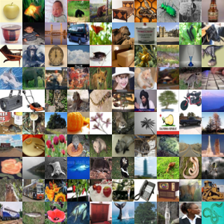
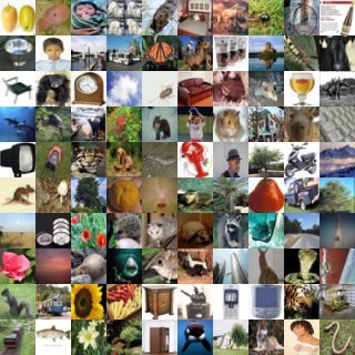
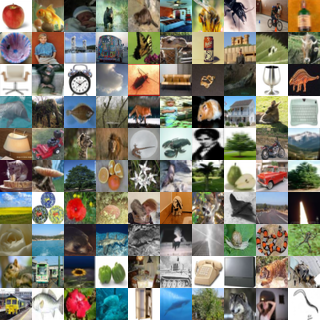
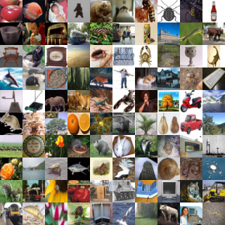
Figure 14: 400 labeled CIFAR100 samples organized into 4 image blocks where each image block is a set of 100 images corresponding to 100 classes. For 100 and 200 labeled samples, the first block and the first two blocks are considered, respectively.

Figure 15: Indices in the training set of the images in Fig. 14

References

- [1] Yuki Markus Asano, Christian Rupprecht, and Andrea Vedaldi. Self-labelling via simultaneous clustering and representation learning. arXiv preprint arXiv:1911.05371, 2019.
- [2] David Berthelot, Nicholas Carlini, Ekin D Cubuk, Alex Kurakin, Kihyuk Sohn, Han Zhang, and Colin Raffel. Remixmatch: Semi-supervised learning with distribution alignment and augmentation anchoring. arXiv preprint arXiv:1911.09785, 2019.
- [3] David Berthelot, Nicholas Carlini, Ian Goodfellow, Nicolas Papernot, Avital Oliver, and Colin A Raffel. Mixmatch: A holistic approach to semi-supervised learning. In Advances in Neural Information Processing Systems, pages 5050–5060, 2019.
- [4] Mathilde Caron, Piotr Bojanowski, Armand Joulin, and Matthijs Douze. Deep clustering for unsupervised learning of visual features. In Proceedings of the European Conference on Computer Vision (ECCV), pages 132–149, 2018.
- [5] Mathilde Caron, Ishan Misra, Julien Mairal, Priya Goyal, Piotr Bojanowski, and Armand Joulin. Unsupervised learning of visual features by contrasting cluster assignments. arXiv preprint arXiv:2006.09882, 2020.
- [6] Jianlong Chang, Yiwen Guo, Lingfeng Wang, Gaofeng Meng, Shiming Xiang, and Chunhong Pan. Deep discriminative clustering analysis. arXiv preprint arXiv:1905.01681, 2019.
- [7] Jianlong Chang, Lingfeng Wang, Gaofeng Meng, Shiming Xiang, and Chunhong Pan. Deep adaptive image clustering. In Proceedings of the IEEE international conference on computer vision, pages 5879–5887, 2017.
- [8] Ting Chen, Simon Kornblith, Mohammad Norouzi, and Geoffrey Hinton. A simple framework for contrastive learning of visual representations. arXiv preprint arXiv:2002.05709, 2020.
- [9] Adam Coates, Andrew Ng, and Honglak Lee. An analysis of single-layer networks in unsupervised feature learning. In Proceedings of the fourteenth international conference on artificial intelligence and statistics, pages 215–223. JMLR Workshop and Conference Proceedings, 2011.
- [10] Ekin D Cubuk, Barret Zoph, Jonathon Shlens, and Quoc V Le. Randaugment: Practical data augmentation with no separate search. arXiv preprint arXiv:1909.13719, 2019.
- [11] Jia Deng, Wei Dong, Richard Socher, Li-Jia Li, Kai Li, and Li Fei-Fei. Imagenet: A large-scale hierarchical image database. In 2009 IEEE conference on computer vision and pattern recognition, pages 248–255. Ieee, 2009.
- [12] Alexey Dosovitskiy, Jost Tobias Springenberg, Martin Riedmiller, and Thomas Brox. Discriminative unsupervised feature learning with convolutional neural networks. In Proceedings of the 27th International Conference on Neural Information Processing Systems-Volume 1, pages 766–774, 2014.
- [13] Prasoon Goyal, Zhiting Hu, Xiaodan Liang, Chenyu Wang, Eric P Xing, and Carnegie Mellon. Nonparametric variational auto-encoders for hierarchical representation learning. In ICCV, pages 5104–5112, 2017.
- [14] Michael Gutmann and Aapo Hyvärinen. Noise-contrastive estimation: A new estimation principle for unnormalized statistical models. In Proceedings of the Thirteenth International Conference on Artificial Intelligence and Statistics, pages 297–304. JMLR Workshop and Conference Proceedings, 2010.
- [15] Raia Hadsell, Sumit Chopra, and Yann LeCun. Dimensionality reduction by learning an invariant mapping. In 2006 IEEE Computer Society Conference on Computer Vision and Pattern Recognition (CVPR’06), volume 2, pages 1735–1742. IEEE, 2006.
- [16] Kaiming He, Haoqi Fan, Yuxin Wu, Saining Xie, and Ross Girshick. Momentum contrast for unsupervised visual representation learning. In Proceedings of the IEEE/CVF Conference on Computer Vision and Pattern Recognition, pages 9729–9738, 2020.
- [17] Kaiming He, Xiangyu Zhang, Shaoqing Ren, and Jian Sun. Deep residual learning for image recognition. In Proceedings of the IEEE conference on computer vision and pattern recognition, pages 770–778, 2016.
- [18] R Devon Hjelm, Alex Fedorov, Samuel Lavoie-Marchildon, Karan Grewal, Phil Bachman, Adam Trischler, and Yoshua Bengio. Learning deep representations by mutual information estimation and maximization. arXiv preprint arXiv:1808.06670, 2018.
- [19] Jiabo Huang, Shaogang Gong, and Xiatian Zhu. Deep semantic clustering by partition confidence maximisation. In Proceedings of the IEEE/CVF Conference on Computer Vision and Pattern Recognition, pages 8849–8858, 2020.
- [20] Xu Ji, João F Henriques, and Andrea Vedaldi. Invariant information clustering for unsupervised image classification and segmentation. In Proceedings of the IEEE/CVF International Conference on Computer Vision, pages 9865–9874, 2019.
- [21] Zhuxi Jiang, Yin Zheng, Huachun Tan, Bangsheng Tang, and Hanning Zhou. Variational deep embedding: An unsupervised and generative approach to clustering. In Proceedings of the 26th International Joint Conference on Artificial Intelligence, pages 1965–1972, 2017.
- [22] Diederik P Kingma and Max Welling. Auto-encoding variational bayes. arXiv preprint arXiv:1312.6114, 2013.
- [23] Alex Krizhevsky. Learning multiple layers of features from tiny images. 2009.
- [24] Samuli Laine and Timo Aila. Temporal ensembling for semi-supervised learning. arXiv preprint arXiv:1610.02242, 2016.
- [25] Dong-Hyun Lee. Pseudo-label: The simple and efficient semi-supervised learning method for deep neural networks. In Workshop on challenges in representation learning, ICML, volume 3, page 2, 2013.
- [26] Junnan Li, Pan Zhou, Caiming Xiong, Richard Socher, and Steven CH Hoi. Prototypical contrastive learning of unsupervised representations. arXiv preprint arXiv:2005.04966, 2020.
- [27] Yunfan Li, Peng Hu, Zitao Liu, Dezhong Peng, Joey Tianyi Zhou, and Xi Peng. Contrastive clustering. arXiv preprint arXiv:2009.09687, 2020.
- [28] Ilya Loshchilov and Frank Hutter. SGDR: Stochastic gradient descent with warm restarts. arXiv preprint arXiv:1608.03983, 2016.
- [29] David McAllester and Karl Stratos. Formal limitations on the measurement of mutual information. In International Conference on Artificial Intelligence and Statistics, pages 875–884. PMLR, 2020.
- [30] Tomas Mikolov, Ilya Sutskever, Kai Chen, Greg S Corrado, and Jeff Dean. Distributed representations of words and phrases and their compositionality. Advances in Neural Information Processing Systems, 26:3111–3119, 2013.
- [31] Ishan Misra and Laurens van der Maaten. Self-supervised learning of pretext-invariant representations. In Proceedings of the IEEE/CVF Conference on Computer Vision and Pattern Recognition, pages 6707–6717, 2020.
- [32] Andriy Mnih and Yee Whye Teh. A fast and simple algorithm for training neural probabilistic language models. In Proceedings of the 29th International Coference on International Conference on Machine Learning, pages 419–426, 2012.
- [33] Aaron van den Oord, Yazhe Li, and Oriol Vinyals. Representation learning with contrastive predictive coding. arXiv preprint arXiv:1807.03748, 2018.
- [34] Sungwon Park, Sungwon Han, Sundong Kim, Danu Kim, Sungkyu Park, Seunghoon Hong, and Meeyoung Cha. Improving unsupervised image clustering with robust learning. arXiv preprint arXiv:2012.11150, 2020.
- [35] Ben Poole, Sherjil Ozair, Aaron Van Den Oord, Alex Alemi, and George Tucker. On variational bounds of mutual information. In International Conference on Machine Learning, pages 5171–5180, 2019.
- [36] Kihyuk Sohn, David Berthelot, Chun-Liang Li, Zizhao Zhang, Nicholas Carlini, Ekin D Cubuk, Alex Kurakin, Han Zhang, and Colin Raffel. Fixmatch: Simplifying semi-supervised learning with consistency and confidence. arXiv preprint arXiv:2001.07685, 2020.
- [37] Jiaming Song and Stefano Ermon. Understanding the limitations of variational mutual information estimators. arXiv preprint arXiv:1910.06222, 2019.
- [38] Antti Tarvainen and Harri Valpola. Mean teachers are better role models: Weight-averaged consistency targets improve semi-supervised deep learning results. In Advances in Neural Information Processing Systems, pages 1195–1204, 2017.
- [39] Yonglong Tian, Dilip Krishnan, and Phillip Isola. Contrastive multiview coding. arXiv preprint arXiv:1906.05849, 2019.
- [40] Wouter Van Gansbeke, Simon Vandenhende, Stamatios Georgoulis, Marc Proesmans, and Luc Van Gool. Scan: Learning to classify images without labels. In European Conference on Computer Vision, pages 268–285. Springer, 2020.
- [41] Jianlong Wu, Keyu Long, Fei Wang, Chen Qian, Cheng Li, Zhouchen Lin, and Hongbin Zha. Deep comprehensive correlation mining for image clustering. In Proceedings of the IEEE/CVF International Conference on Computer Vision, pages 8150–8159, 2019.
- [42] Zhirong Wu, Yuanjun Xiong, Stella X Yu, and Dahua Lin. Unsupervised feature learning via non-parametric instance discrimination. In Proceedings of the IEEE Conference on Computer Vision and Pattern Recognition, pages 3733–3742, 2018.
- [43] Junyuan Xie, Ross Girshick, and Ali Farhadi. Unsupervised deep embedding for clustering analysis. In International conference on machine learning, pages 478–487. PMLR, 2016.
- [44] Jiahao Xie, Xiaohang Zhan, Ziwei Liu, Yew Soon Ong, and Chen Change Loy. Delving into inter-image invariance for unsupervised visual representations. arXiv preprint arXiv:2008.11702, 2020.
- [45] Qizhe Xie, Zihang Dai, Eduard Hovy, Minh-Thang Luong, and Quoc V Le. Unsupervised data augmentation for consistency training. 2019.
- [46] Bo Yang, Xiao Fu, Nicholas D Sidiropoulos, and Mingyi Hong. Towards k-means-friendly spaces: Simultaneous deep learning and clustering. In international conference on machine learning, pages 3861–3870. PMLR, 2017.
- [47] Jianwei Yang, Devi Parikh, and Dhruv Batra. Joint unsupervised learning of deep representations and image clusters. In Proceedings of the IEEE conference on computer vision and pattern recognition, pages 5147–5156, 2016.
- [48] Linxiao Yang, Ngai-Man Cheung, Jiaying Li, and Jun Fang. Deep clustering by gaussian mixture variational autoencoders with graph embedding. In Proceedings of the IEEE/CVF International Conference on Computer Vision, pages 6440–6449, 2019.
- [49] Mang Ye, Xu Zhang, Pong C Yuen, and Shih-Fu Chang. Unsupervised embedding learning via invariant and spreading instance feature. In Proceedings of the IEEE/CVF Conference on Computer Vision and Pattern Recognition, pages 6210–6219, 2019.
- [50] Yaodong Yu, Kwan Ho Ryan Chan, Chong You, Chaobing Song, and Yi Ma. Learning diverse and discriminative representations via the principle of maximal coding rate reduction. Advances in Neural Information Processing Systems, 33, 2020.
- [51] Xiaohang Zhan, Jiahao Xie, Ziwei Liu, Yew-Soon Ong, and Chen Change Loy. Online deep clustering for unsupervised representation learning. In Proceedings of the IEEE/CVF Conference on Computer Vision and Pattern Recognition, pages 6688–6697, 2020.
- [52] Hongyi Zhang, Moustapha Cisse, Yann N Dauphin, and David Lopez-Paz. mixup: Beyond empirical risk minimization. arXiv preprint arXiv:1710.09412, 2017.
- [53] Huasong Zhong, Chong Chen, Zhongming Jin, and Xian-Sheng Hua. Deep robust clustering by contrastive learning. arXiv preprint arXiv:2008.03030, 2020.
- [54] Chengxu Zhuang, Alex Lin Zhai, and Daniel Yamins. Local aggregation for unsupervised learning of visual embeddings. In Proceedings of the IEEE/CVF International Conference on Computer Vision, pages 6002–6012, 2019.