Sub-Sharvin conductance and enhanced shot noise in doped graphene

Abstract

Ideal Sharvin contact in a multimode regime shows the conductance $G\approx{}G_{\rm Sharvin}=g_{0}k_{F}{}W/\pi$ (with $g_{0}$ the conductance quantum, $k_{F}$ the Fermi momentum, and $W$ the contact width) accompanied by strongly suppressed shot-noise quantified by small Fano factor $F\approx{}0$. For ballistic graphene away from the charge-neutrality point the sub-Sharvin transport occurs, characterised by suppressed conductance $G\approx{}(\pi/4)\,G_{\rm Sharvin}$ and enhanced shot noise $F\approx{}1/8$. All these results can be derived from a basic model of quantum scattering, involving assumptions of infinite height and perfectly rectangular shape of the potential barrier in the sample. Here we have carried out the numerical analysis of the scattering on a family of smooth barriers of finite height interpolating between parabollic and rectangular shapes. We find that tuning the barrier shape one can modify the asymmetry between electron- and hole-doped systems. For electronic dopings, the system crosses from Sharvin to sub-Sharvin transport regime (indicated by both the conductance and the Fano factor) as the potential becomes closer to the rectangular shape. In contrast, for hole dopings, the conductivity is strongly suppressed when the barrier is parabolic and slowly converges to $G\approx{}(\pi/4)\,G_{\rm Sharvin}$ as the potential evolves towards rectangular shape. In such a case the Sharvin transport regime is inaccessible, shot noise is generically enhanced (with much slower convergence to $F\approx{}1/8$) comparing to the electron-doped case, and aperiodic oscillations of both $G$ and $F$ are prominent due to the formation of quasibound states.

I Introduction

Soon after the isolation of monolayer graphene Nov04 experimental and theoretical physicists have reexamined classical effects from mesoscopic phycics Nov05 ; Zha05 ; Rus10 ; Lin08 ; Tom11 ; Pal12 ; Ryc13 ; Hua18 ; Zen19 . In ballistic graphene ribbons Lin08 or constrictions Tom11 , showing conductance quantization, electrical conductance approaches the fundamental upper bound given by the Sharvin formula Sha65 ; Bee91 . A few years ago, ultraclean graphene samples exhibiting a viscous charge flow due to electron-electron interactions Luc18 allowed to detect the conductance exceeding the Sharvin bound Guo17 ; Kum17 .

Since the spectrum of excitations in graphene consists of two conical bands and is described by a two-dimensional analog of the relativistic Dirac equation Mcc56 ; Sem84 ; Div84 , several novel effects can be identified even at low temperatures, where interactions become negligible and ballistic (or Landauer-Büttiker) transport regime is restored Kat06 ; Two06 ; Mia07 ; Dan08 ; Ryc10 ; Ric15 ; Kum18 . For instance, the phenomenon of Klein tunneling Kat12 manifests itself via the universal conductivity ($\sigma_{0}=4e^{2}/\pi{}h$, with the electron charge $-e$ and the Planck constant $h$) and the so-called pseudodiffusive shot noise power (quantified by the Fano factor $F=1/3$) Two06 ; Mia07 ; Dan08 provided that carrier concentration is close to the charge-neutrality point.

Although several features of ballistic graphene may also be observed in other two-dimensional systems Eza13 ; Eza15 ; Rze20 universal conductivity seems to be the unique feature of graphene, having no direct analog even in bilayer graphene Sus20 .

Remarkably, in the universal-conductivity range (for a rectangular sample, it is further required that the width $W\gg{}L$ with $L$ being the length, see Ref. Ryc09 ) the conductance is enhanced due to the transport via evanescent waves, while the shot noise is suppressed. However, tuning the carrier concentration away from the charge-neutrality point, results in the Fano factor approaching values in a range of $F\approx{}0.10\div{}0.15$ Two06 ; Dan08 , being significantly greater then $F\approx{}0$ expected for a ballistic system. The conductance is difficult to be determined experimentally due to resistances of contacts, but the simple analytical discussion leads to the value reduced by a factor of $\pi/4$ compared to the Sharvin formula in the high-doping limit Par21 ; Ryc21 . (Same analysis leads to the Fano factor converging to $F\rightarrow{}1/8$.)

The purpose of this work is to investigate numerically, how the conductance and Fano factor for a ballistic graphene sample behave as functions of doping supposing that the electrostatic potential barrier is smooth (i.e., potential varies slowly on the scale of atomic separation). Similar problems were addressed previously Par21 ; Sil07 ; Che06 ; Cay09 , but here we focus on the effects of the potential profile, which is gradually tuned from a parabolic to a rectangular shape (see Fig. 1), on the selected transport properties.

The paper is organized as follows. In Sec. II, we present the details of our numerical approach. The key results for a rectangular barrier are summarized in Sec. III. Our main results, concerning the conductance and Fano factor for smooth potentials are presented in Sec. IV. The conclusions are given in Sec. V.

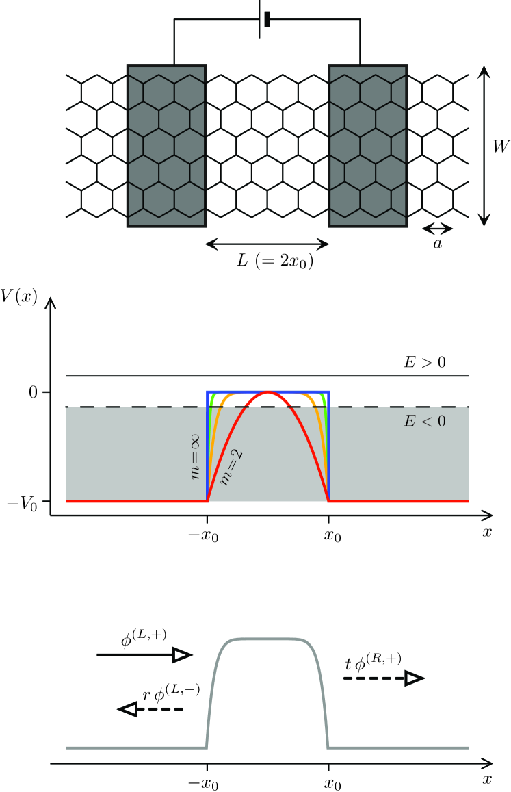
Figure 1: Top: Schematic of a graphene strip of width $W$, contacted by two electrodes (dark areas) at a distance $L$. A voltage source drives a current through the strip. A separate gate electrode (not shown) allows to tune the carrier concentration around the neutrality point. The lattice parameter $a=0.246\,$nm is also shown. Middle: Electrostatic potential profiles given by Eq. (4) with $m=2,8,32,$ and $m=\infty$ (i.e., the rectangular barrier). The Fermi energy $E$ is defined with respect to the top of a barrier. $E>0$ corresponds to unipolar n-n-n doping in the device; for $E<0$, a n-p-n structure is formed. Bottom: A symbolic representation of the incident and reflected waves in left electrode ($x<-x_{0}$) and the transmitted wave in right electrode ($x>x_{0}$) with the amplitudes $r$ and $t$.

II Model and methods

We start from the scattering problem for massless Dirac fermions in graphene at the energy $E$, in case when the electrostatic potential energy depends only on the $x$ coordinate, i.e., $V\equiv{}V(x)$. The wave equation can be written as

$$\left[v_{F}\,\mbox{\boldmath$p$}\cdot\mbox{\boldmath$\sigma$}+V(x)\right]\Psi=E\Psi,$$ (1)

where $v_{F}=\sqrt{3}\,t_{0}a/(2\hbar)\approx{}10^{6}\,$m$/$s is the energy-independent Fermi velocity in graphene (with $t_{0}=2.7\,$eV the nearest-neighbor hopping integral and $a=0.246$ the lattice parameter), $\mbox{\boldmath$p$}=(p_{x},p_{y})$ is the in-plane momentum operator with $p_{j}=-i\hbar{}\partial_{j}$, and $\mbox{\boldmath$\sigma$}=(\sigma_{x},\sigma_{y})$ with $\sigma_{j}$ being the Pauli matrices. Taking the wavefunction in a form $\Psi=\phi(x)e^{ik_{y}y}$, with $\phi(x)=(\phi_{a},\phi_{b})^{T}$ and $k_{y}$ the transverse wavenumber, brought us to the system of ordinary differential equations for the spinor components

$$\phi_{a}^{\prime} =k_{y}\phi_{a}+i\frac{E-V(x)}{\hbar{}v_{F}}\phi_{b},$$ (2)

$$\phi_{b}^{\prime} =i\frac{E-V(x)}{\hbar{}v_{F}}\phi_{a}-k_{y}\phi_{b}.$$ (3)

In a general case of $k_{y}\neq{}0$, Eqs. (2,3) need to be integrated numerically Sil07 . If one assumes the so-called infinite-mass boundary conditions Ber87 at $y=0$ and $y=W$, in the momentum $k_{y}$ gets quantized $k_{y}^{(n)}=\pi{}(n+\frac{1}{2})/W$, with $n=0,1,2,\dots$, Two06 . This form is used throughout the paper. (In the limit of $W\gg{}L$, one can also treat $k_{y}$ as a as a continuous variable.)

The electrostatic potential energy is chosen as

$$V(x)=-V_{0}\times\begin{cases}\,\left|x/x_{0}\right|^{m}&\text{if }\ |x|\leqslant x_{0},\\ \,1&\text{if }\ |x|>x_{0},\end{cases}$$ (4)

such that changing the value of $m$ tunes the potential from parabolic shape ($m=2$) to rectangular shape ($m\rightarrow\infty$). Above we use a parameter $x_{0}=L/2$, with $L$ the sample length. The potential given by Eq. (4) is continuous and constant in the leads ($x<-L/2$ or $x>L/2$).

The basis solutions in the leads, for $E>-V_{0}$, are

$$\phi^{(+)}=\left(\begin{matrix}1\\ e^{i\theta}\\ \end{matrix}\right)e^{iK_{x}{}x},\ \ \ \ \phi^{(-)}=\left(\begin{matrix}1\\ -e^{-i\theta}\\ \end{matrix}\right)e^{-iK_{x}{}x},$$ (5)

where $e^{i\theta}=(K_{x}+ik_{y})/K$, $K=(E+V_{0})/\hbar{}v_{F}$, and $K_{x}=\sqrt{K^{2}-k_{y}^{2}}$. Transverse momentum is conserved in the scattering leadfoo , so the value of the quantum number $k_{y}$ is the same for both leads and the sample area. Supposing scattering from the left direction ($x=-\infty$), the wavefunctions in the left ($L$) and right ($R$) lead can be written as

$$\phi_{E,k_{y}}^{(L)}=\phi^{(+)}+r\phi^{(-)},\ \ \ \ \ \phi_{E,k_{y}}^{(R)}=t\phi^{(+)},$$ (6)

where we have defined the reflection ($r$) and transmission ($t$) amplitudes.

For the sample area ($-L/2<x<L/2$) the wavefunction takes a form

$$\phi_{E,k_{y}}^{(c)}=A\phi^{(1)}+B\phi^{(2)},$$ (7)

where $\phi^{(1)}$, $\phi^{(2)}$ denote the two linearly-independent solutions of Eqs. (2,3), which can be obtained numerically choosing the initial conditions, say $\left.\phi^{(1,2)}\right|_{x=-x_{0}}=(1,\pm{}1)^{T}$, and $A$, $B$ are arbitrary complex coefficients.

The matching conditions for $x=\pm{}x_{0}$, namely

$$\phi_{E,k_{y}}^{(L)}=\left.\phi_{E,k_{y}}^{(c)}\right|_{x=-x_{0}}\ \ \ \text{and}\ \ \ \phi_{E,k_{y}}^{(c)}=\left.\phi_{E,k_{y}}^{(R)}\right|_{x=x_{0}},$$ (8)

immediately leads to the linear system of equations

$$\left[\begin{matrix}\phi_{a}^{(-)}(-x_{0})&-\phi_{a}^{(1)}(-x_{0})&-\phi_{a}^{(2)}(-x_{0})&0\\ \phi_{b}^{(-)}(-x_{0})&-\phi_{b}^{(1)}(-x_{0})&-\phi_{b}^{(2)}(-x_{0})&0\\ 0&-\phi_{a}^{(1)}(x_{0})&-\phi_{a}^{(2)}(x_{0})&\phi_{a}^{(+)}(x_{0})\\ 0&-\phi_{b}^{(1)}(x_{0})&-\phi_{b}^{(2)}(x_{0})&\phi_{b}^{(+)}(x_{0})\\ \end{matrix}\right]\left[\begin{matrix}r\\ A\\ B\\ t\\ \end{matrix}\right]=\left[\begin{matrix}-\phi_{a}^{(+)}(-x_{0})\\ -\phi_{b}^{(+)}(-x_{0})\\ 0\\ 0\\ \end{matrix}\right],$$ (9)

where we have explicitly written the spinor components and omitted repeating indices $(E,k_{y})$ for clarity.

Solving Eq. (9), one finds the transmission amplitude $t$ for a given $E$ and $k_{y}$, and the corresponding transmission probability $T_{k_{y}}(E)=|t|^{2}$. The conductance and Fano factor follow by summing over the modes,

$$G=g_{0}\sum_{n=0}^{N-1}T_{n},\ \ \ \ \ \ F=\frac{\sum_{n=0}^{N-1}T_{n}(1-T_{n})}{\sum_{n=0}^{N-1}T_{n}},$$ (10)

with $g_{0}=4e^{2}/h$ (the factor $4$ accounts for spin and valley degeneracy), $T_{n}=T_{k_{y}}(E)$ for $k_{y}^{(n)}=\pi{}(n+\frac{1}{2})/W$, and $N=\lfloor{}WK/\pi\rfloor$ being the number of propagating modes in the leads, see Eq. (5). In the linear-response regime, imposed in Eq. (10), the energy $E$ is equivalent to the Fermi energy Naz09 ; for $E>0$ the sample and the leads show an unipolar (n-n-n) doping, for $-V_{0}<E<0$ we have n-p-n structure with two interfaces separating the central region and the leads (see Fig. 1).

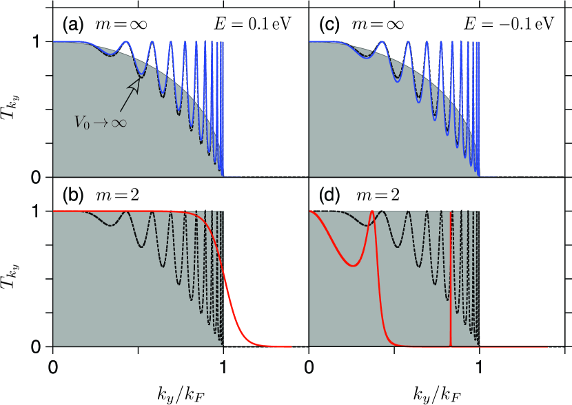
Figure 2: Transmission probability as a function of the transverse momentum $k_{y}$ (specified as a fraction of $k_{F}=|E|/\hbar{}v_{F}$) at the Fermi energies $E=0.1\,$eV (a,b) and $E=-0.1\,$eV (c,d). The barrier length is $L=200\,$nm. Solid lines present results obtained numerically for the potential given by Eq. (4) with $V_{0}=t_{0}/2=1.35\,$eV and $m=\infty$ or $m=2$ (specified at each panel). Dashed lines depict exact expression [see Eq. 11] for infinite rectangular barrier (a–d). Shaded areas mark the approximations given by Eq. (13) (a,c) or by the step function $T_{k_{y}}\approx\Theta\left(k_{F}-|k_{y}|\right)$ (b,d).

III The rectangular barrier versus Sharvin contact

Before presenting the numerical results for smooth barriers, we first recall analytic expressions for a rectangular barrier of infinite height, corresponding to $m\rightarrow{}\infty$, $V_{0}\rightarrow{}\infty$ in Eq. (4). Adapting the notation of Ref. Ryc09 , the transmission probability can be written as

$$T_{k_{y}}(E)=\left[1+\left(\dfrac{k_{y}}{\varkappa}\right)^{2}\sin^{2}\left(\varkappa{}\,L\right)\right]^{-1},$$ (11)

where

$$\varkappa=\begin{cases}\sqrt{k_{F}^{2}-k_{y}^{2}},&\text{for }\ |k_{y}|\leqslant{}k_{F},\\ i\sqrt{k_{y}^{2}-k_{F}^{2}},&\text{for }\ |k_{y}|>k_{F},\\ \end{cases}$$ (12)

and the Fermi wavenumber $k_{F}=|E|/(\hbar{}v_{F})$.

In Fig. 2, we compare the results obtained from Eq. (11) for the length fixed at $L=200\,$nm (black dashed lines) with the results of our numerical approach [see Eqs. (2–9)] for $V_{0}=t_{0}/2$, and $m=\infty$ or $m=2$ (blue solid or red solid lines). Here, continuous $k_{y}$ corresponds to the $W\gg{}L$ limit. (We further limit the discussion to $k_{y}\geqslant{}0$, as the mirror symmetry guarantees that $T_{k_{y}}=T_{-k_{y}}$ for any case.) The Fermi energy is $E=0.1\,$eV in Figs. 2a and 2b, or $E=-0.1\,$eV in Figs. 2c and 2d.

In is clear from Figs. 2a and 2c that the results a finite and infinite $V_{0}$ are very close to each other, as long as $|E|\ll{}V_{0}$. Analytic results for $V_{0}\rightarrow\infty$ are invariant upon the particle-hole transformation ($E\leftrightarrow{}-E$); for a finite $V_{0}$, this invariance is only approximate, since the number of propagating modes in the leads per unit width, $N/W\approx(E+V_{0})/(\pi\hbar{}v_{F})$ changes upon $E\leftrightarrow{}-E$. In both cases of $E>0$ and $E<0$ we observe fast, aperiodic oscillations of $T_{k_{y}}$ with $k_{y}$ approaching $k_{F}$, and a sudden decay for $k_{y}>k_{F}$, signalling that the role of evanescent waves is negligible (notice that $k_{F}{}L\gg{}1$).

For the case of a finite and smooth parabolic barrier, a striking particle-hole asymmetry is visible, see Figs. 2b and 2d. For $E>0$, we have a smooth crossover from $T_{k_{y}}\approx{}1$ to $T_{k_{y}}\approx{}0$ near $k_{y}=k_{F}$, resembling the well-known solution for Schrödinger electrons Kem35 . For $E<0$, the transmission is strongly suppressed, except from the resonances due to quasibound states Sil07 .

Let us now comment on obtaining simple, analytically tractable estimates of the conductance and Fano factor.

A closer look at Eq. (11) allows one to find out that, when calculating the transport properties from Eq. (10) for $k_{F}{}L\gg{}1$, summing over the modes averages out fast oscillations originating from $\sin^{2}(\varkappa{}L)$, and exact transmission probability may be approximated by

$$\left(T_{k_{y}}\right)_{\rm approx} =\frac{1}{\pi}\int_{0}^{\pi}\frac{d\varphi}{1+\left(k_{y}^{2}/\varkappa^{2}\right)\sin^{2}\varphi}$$

$$=\sqrt{1-\left(k_{y}/k_{F}\right)^{2}},$$ (13)

for $|k_{y}|\leqslant{}k_{F}$; otherwise, $\left(T_{k_{y}}\right)_{\rm approx}=0$. In particular, for the conductance $G$ in the $W\gg{}L$ limit, we can put

$$G\approx{}\frac{g_{0}{}W}{\pi}\int_{0}^{\infty}dk_{y}\left(T_{k_{y}}\right)_{\rm approx}=\frac{\pi}{4}\,G_{\rm Sharvin},$$ (14)

with $G_{\rm Sharvin}=g_{0}k_{F}{}W/\pi$. It is worth to notice that $G\approx{}G_{\rm Sharvin}$ corresponds to $T_{k_{y}}\approx\Theta\left(k_{F}-|k_{y}|\right)$, where $\Theta(x)$ denotes the Heaviside step function — see shaded areas in Figs. 2(c) and 2(d). — representing a reasonable approximation in the $m=2$ (parabolic barrier) and $E>0$ case, at least if one focuses on the area under the $T_{k_{y}}$ plot. In the remaining parts of this paper, $G$ close to the approximation given by Eq. (14) is called the sub-Sharvin conductance.

For the Fano factor, see Eq. (10), we need to employ both Eq. (13) and the analogous expression for $T_{k_{y}}^{2}$, namely

$$\left(T_{k_{y}}^{2}\right)_{\rm approx} =\frac{1}{\pi}\int_{0}^{\pi}\frac{d\varphi}{\left[1+\left(k_{y}^{2}/\varkappa^{2}\right)\sin^{2}\varphi\right]^{2}}$$

$$=\sqrt{1-\left(\frac{k_{y}}{k_{F}}\right)^{2}}\left[1-\frac{1}{2}\left(\frac{k_{y}}{k_{F}}\right)^{2}\right],$$ (15)

for $|k_{y}|\leqslant{}k_{F}$, or $\left(T_{k_{y}}^{2}\right)_{\rm approx}=0$ for $|k_{y}|>k_{F}$. In turn, we immediately obtain

$$F\approx{}1-\frac{\int_{0}^{\infty}dk_{y}\left(T_{k_{y}}^{2}\right)_{\rm approx}}{\int_{0}^{\infty}dk_{y}\left(T_{k_{y}}\right)_{\rm approx}}=\frac{1}{8},$$ (16)

constituting a hallmark of the sub-Sharvin transport regime.

For the sake of completeness, we also recal the results of Refs. Kat06 ; Two06 for $E=0$. In such a case, Eq. (11) reduces to

$$T_{k_{y}}(0)=\frac{1}{\cosh^{2}\left(k_{y}{}L\right)},$$ (17)

and integrations over $k_{y}$, analogous to the performed in Eqs. (14) and (16), leads to

$$G_{\rm min}=\frac{g_{0}W}{\pi{}L},\ \ \ \ \ \text{and }\ \ \ \ \ F_{\rm max}=\frac{1}{3},$$ (18)

indicating the pseudodiffusive transport regime. (It is further denoted in Eq. (18) that $G$ has a minimum, whereas $F$ has a maximum at $E=0$.) The energy range $-E_{\rm diff}<E<E_{\rm diff}$, in which the pseudodiffusive transport prevails the ballistic transport, can roughly be estimated comparing $G_{\rm min}=G_{\rm Sharvin}(\pm{}E_{\rm diff})$, what leads to

$$E_{\rm diff}=\frac{\hbar{}v_{F}}{L}\approx{}2.9\,\text{meV}\ \ \text{for }\ L=200\,\text{nm}.$$ (19)

The above is close to a familiar energy uncertainty in quantum mechanics, since the ballistic time of flight is $\Delta{}t\sim{}L/v_{F}$ (up to the order of magnitude).

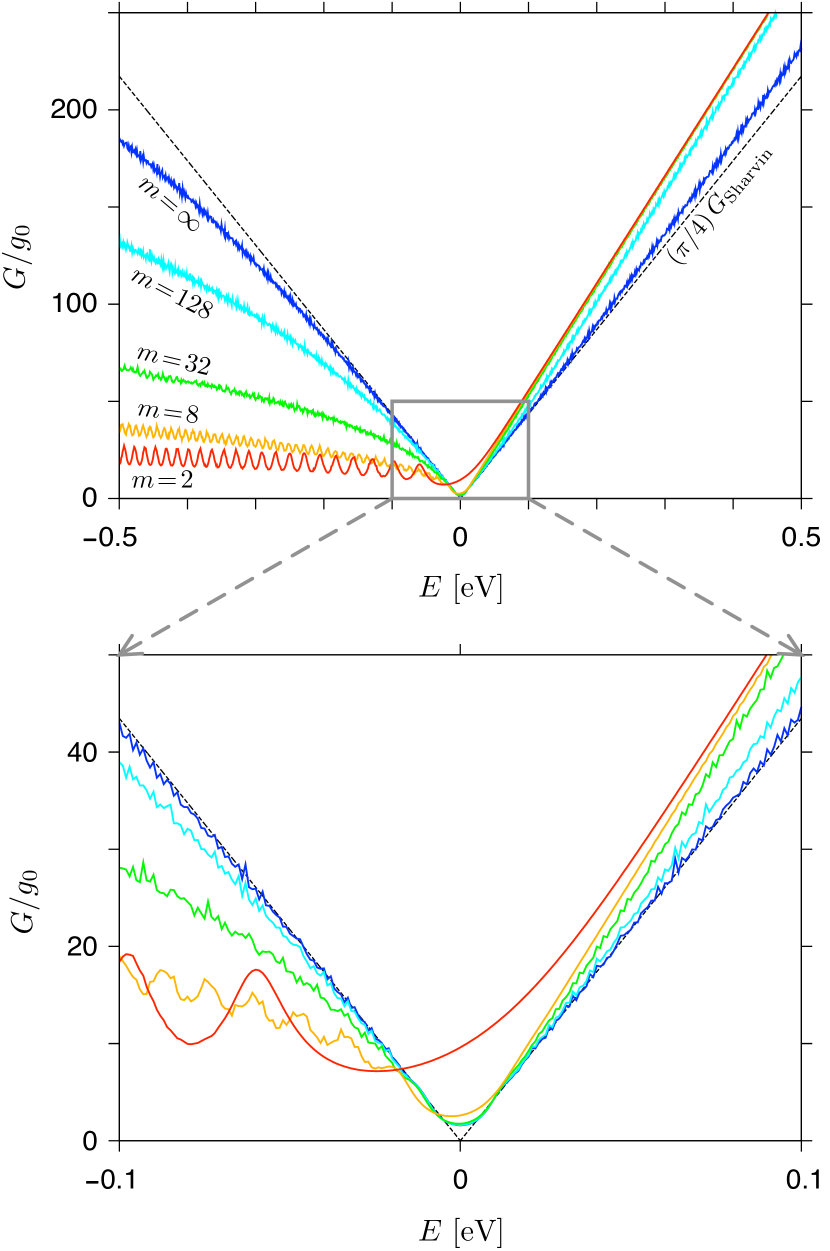
Figure 3: Conductance as a function of the Fermi energy for the system of Fig. 1. The parameters are: $W=5\,L=1000\,$nm, $V_{0}=t_{0}/2=1.35\,$eV. The exponent $m$ in Eq. (4) is specified for each dataset (solid lines). Dashed line depicts the sub-Sharvin conductance given by Eq. (14). (The values of $G_{\rm Sharvin}$ are not shown, as they closely follow the numerical results for $m=2$.) Bottom panel is zoom-in of the data presented in top panel.

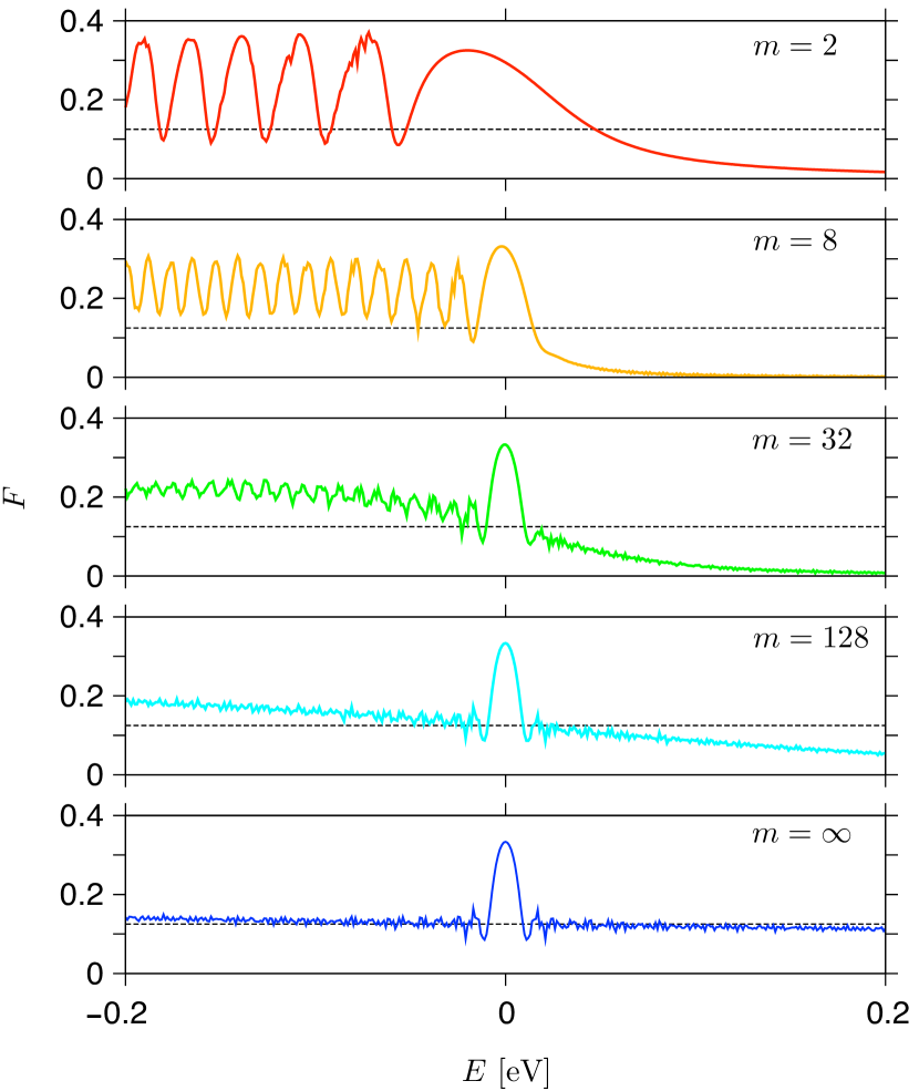
Figure 4: Fano factor as a function of the Fermi energy for the same system parameters as in Fig. 3 (solid lines). The exponent $m$ in Eq. (4) is varied between the panels. Dashed line at each panel depits the sub-Sharvin value of $F=1/8$, see Eq. (16).

IV Results and discussion

In this Section, we present central results of the paper, concerning the conductance and the Fano factor for a graphene strip depicted in Fig. 1. The numerical calculations are carried out according to Eqs. (2–10), for the system with infinite-mass boundary conditions and the width $W=5\,L=1000\,$nm. The step height in Eq. (4) is $V_{0}=t_{0}/2$ (corresponding to $691\leqslant{}N\leqslant{}802$ propagating modes in the leads for $-0.1\,\text{eV}\leqslant{}E\leqslant{}0.1\,$eV) simfoo .

The evolution of the conductance spectrum with the exponent $m$ in Eq. (4), defining the potential profile, is visualized in Fig. 3 [solid lines]. We focus now on the behavior of $G(E)$ for $|E|\gg{}E_{\rm diff}$, see Eq. (19), since a close vicinity of $E=0$ requires a separate discussion.

Depending on whether the system is unipolar ($E>0$) or contains p-n junctions ($E<0$), different behaviors are observed: For $E>0$, $G(E)$ shows a transition, with growing $m$, from $G_{\rm Sharvin}$ to sub-Sharvin $G\approx{}(\pi/4)\,G_{\rm Sharvin}$ [dashed line]. Comparing the plots with different energy ranges (top and bottom panel in Fig. 3) we immediately notice that the higher the energy, the slower convergence with growing $m$ occurs. In fact, even the results for a rectangular barrier ($m=\infty$) do not match precisely Eq. (14) due to a finite value of $V_{0}$. The deviations are, however, within the scale of Fabry-Perrot oscillations, as long as $|E|\leqslant{}0.1\,$eV. For $E<0$, the conductance is noticeably suppressed for any finite $m$, and shows a slow convergence (from the bottom) to sub-Sharvin values with growing $m$. Contrary to the $E>0$ case, the values of $G>(\pi/4)\,G_{\rm Sharvin}$ are not observed for $E<0$, except from a close surrounding of $E=0$. As a secondary feature of the $E<0$ data, we notice relatively strong conductance oscillations due to resonances with quasibound states.

The above observations are further supported with the evolution of Fano factor presented in Fig. 4. Again, for $|E|\gg{}E_{\rm diff}$, the role of pseudodiffusive transport is irrelevant and the evolution of $F$, with growing $m$, follows one of the two distinct scenarios: For $E>0$, we have a systematic crossover from $F\approx{}0$ to $F\approx{}1/8$; see Eq. (16). In contrast, for $E<0$, strong oscillation of $F$ are first suppressed with increasing $m$, and than — for higher $m$ — slow convergence of a mean to $F\approx{}1/8$ (from the top) becomes visible. Similarly as for the conductance, the particle hole symmetry is only approximate even for $m=\infty$, since the barrier height $V_{0}=t_{0}/2<\infty$.

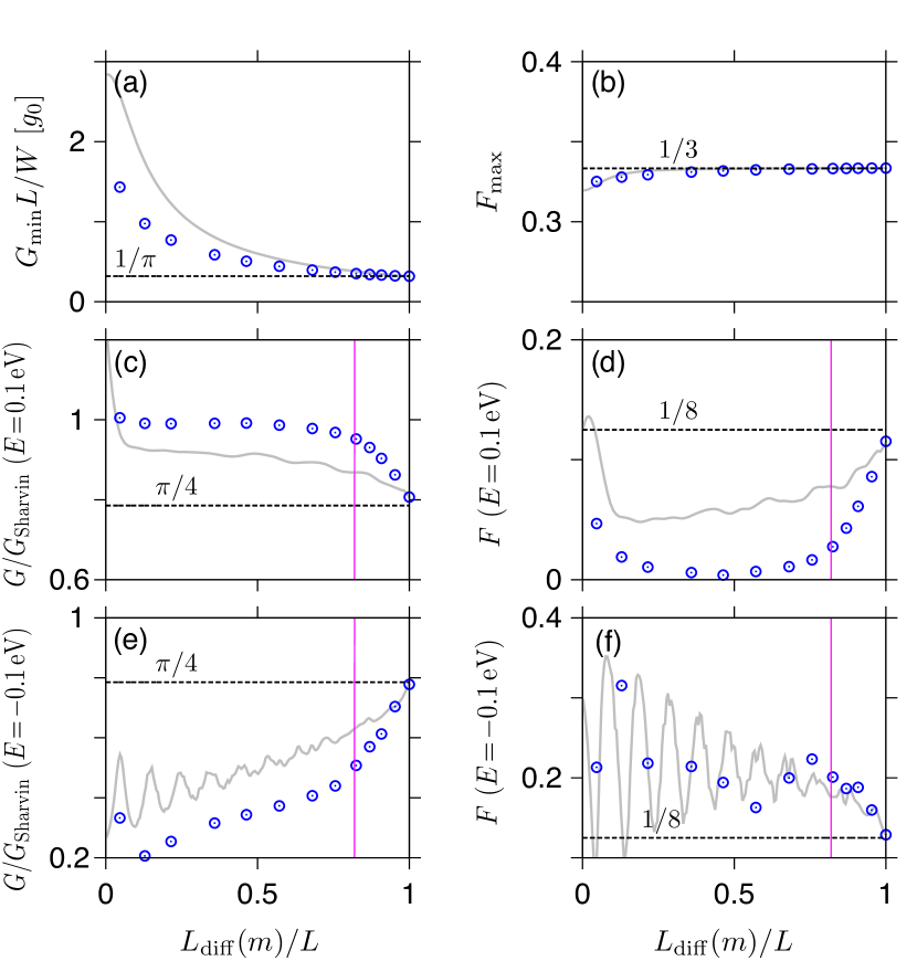
Figure 5: (a–f) Selected characteristics of the datasets presented in Figs. 3 and 4 displayed as functions of the dimensionless $L_{\rm diff}(m)/L$, see Eq. (20). Datapoints: (a) Minimal conductance. (b) Maximal Fano factor. (c) Conductance and (d) Fano factor at $E=0.1\,$eV. (e,f) Same as (c,d) but for $E=-0.1\,$eV. Dashed horizontal lines depict theoretical values for $m\rightarrow\infty$, $V_{0}\rightarrow\infty$, see Eqs. (14), (16), and (18). Vertical lines (c–f) mark a bound on the right-hand side of Eq. (22) for $|E|=0.1\,$eV. Grey solid lines (a–f) show the results for trapezoidal barrier, see Eqs. (23) and (24).

In order to describe the above-presented evolution of $G$ and $F$ upon tuning the potential profile in a quantitative manner, we display now (in Fig. 5) some characteristic values extracted from the curves in Figs. 3 and 4.

Let us focus on the low-energy behavior of $G$ and $F$, which have not been addressed so far in this Section. Using the value of $E_{\rm diff}$ given by Eq. (19), one can define the effective ($m$-dependent) length $L_{\rm diff}$, such that a barrier can be regarded as flat for $-L_{\rm diff}/2<x<L_{\rm diff}/2$. Requesting that $V(\pm{}L_{\rm diff}/2)=-E_{\rm diff}$, one obtains

$$L_{\rm diff}(m)=L\left(\frac{\hbar{}v_{F}}{LV_{0}}\right)^{1/m},$$ (20)

reducing to $L_{\rm diff}(\infty)=L$ for a rectangular barrier. Such a definition allows one to present the results for any $m>0$ in a compact range, i.e. $0<L_{\rm diff}(m)/L\leqslant{}1$.

Both the minimal conductance and the maximal Fano factor, see Figs. 5(a) and 5(b), show rapid convergence (with $L_{\rm diff}/L\rightarrow{}1$) to the values predicted for infinite rectangular barrier, see Eq. (18). In particular, $F_{\rm max}\approx{}0.325$ for the lowest considered $m=2$ (corresponding to $L_{\rm diff}/L\approx{}0.046$). This finding illustrates how the precise value of $F_{\rm max}$ is insensitive to the details of electrostatic potential profile, helping to understand, why experimental values of $F$ are sometimes surprisingly close to $1/3$ Dan08 ; Dic08 ; Kum15 .

Away from the charge-neutrality point, the system characteristics presented in Figs. 5(c)–5(f) show a different behavior. Namely, they generally take values rather distant from predictions given (respectively) in Eqs. (14) and (16), except from a relatively narrow interval near $L_{\rm diff}/L=1$, in which systematic convergence occurs.

A brief explanation is provided below.

For $|E|\gg{}E_{\rm diff}$, the evolution of $G$ and $F$ depends on a mutual relation between the Fermi wavelength $\lambda_{F}(E)=2\pi/k_{F}=h{}v_{F}/|E|$, and the characteristic lenghtscale of a potential jump, which can be defined as $\Delta{}x=(L-L_{\rm diff})/2$, with $L_{\rm diff}$ given by Eq. (20). If

$$\lambda_{F}/2\lesssim\Delta{}x,$$ (21)

the barrier cannot longer be regarded as (even approximately) rectangular. Since $\Delta{}x$ is related to $m$ via $L_{\rm diff}$, Eq. (21) can be rewritten as

$$\frac{L_{\rm diff}}{L}\lesssim{}1-\frac{2\pi\hbar{}v_{F}}{L|E|},$$ (22)

giving $L_{\rm diff}/L\lesssim{}0.82$ for $|E|=0.1\,$eV. The structure of Eq. (22) guarantees that the inequality is always satisfied for $L_{\rm diff}<L$ (i.e., the smooth potential, $m<+\infty$) and sufficiently high $|E|$. In such a case, the measurable quantities deviate from the predictions for a rectangular barrier.

Once the upper bound in Eq. (22) marked with vertical line in Figs. 5(c)–5(f) is exceeded (i.e., $\lambda_{F}>2\Delta{}x$), a systematic convergence of all the considered quantities, with $L_{\rm diff}/L\rightarrow{}1$, to the predictions for a rectangular barrier becomes visible.

Finally, it is worth to compare our results with those corresponding for trapezoidal barrier, discussed in Ref. Par21 . The electrostatic potential energy can be written as

$$V(x)=-V_{0}\times\begin{cases}\,0&\text{if }\ |x|\leqslant x_{1},\\ \,{\displaystyle\frac{|x|-x_{1}}{x_{0}-x_{1}}}&\text{if }\ x_{1}<|x|\leqslant x_{0},\\ \,1&\text{if }\ |x|>x_{0},\end{cases}$$ (23)

with $0\leqslant x_{1}\leqslant x_{0}$, parametrizing the barrier evolution between the limiting cases of triangular ($x_{1}=0$) and rectangular shape ($x_{1}=x_{0}$). In analogy to Eq. (20), we have

$$L_{\rm diff}(x_{1})=2x_{1}+\frac{\hbar{}v_{F}}{LV_{0}}\left(L\!-\!2x_{1}\right)\approx{}2x_{1}.$$ (24)

Taking the same values of $W$, $L$, and $V_{0}$ as before, and varying $x_{1}$, one can easily find that the conductance and Fano factor spectrum evolves in a qualitatively similar manner as the spectra depicted in Figs. 3 and 4. Several quantitative differences can be identified, however, referring to the numerical characteristics presented in Fig. 5 [grey solid lines]. First, for $L_{\rm diff}\ll{}L$ and $E>0$, the conductance significantly exceeds the value of $G_{\rm Sharvin}$, and the Fano factor is also enhanced compared to the smooth potentials; see Figs. 5(c) and 5(d). Most remarkably, the values of $G\approx{}G_{\rm Sharvin}$ and $F\approx{}0$ are never approached for trapezoidal potentials, showing that standard ballistic transport may be restored in bulk graphene ($W\gg{}L$) only for smooth barriers. For $E<0$, the behavior of $G$ and $F$ is similar for smooth and trapezoidal potentials, see Figs. 5(e) and 5(f); some enhancement of $G$ (and slightly faster convergence to sub-Sharvin value with $L_{\rm diff}/L\rightarrow{}1$) can be noticed for trapezoidal barriers.

V Conclusions

We have identified sub-Sharvin transport regime in ballistic graphene, which manifests itself via the suppressed conductivity, $G\approx(\pi/4)\,G_{\rm Sharvin}$ (with $G_{\rm Sharvin}=g_{0}k_{F}{}W/\pi{}$, $g_{0}=4e^{2}/h$ the conductance quantum, $k_{F}$ the Fermi wavenumber, and $W$ the sample width), and the enhanced shot noise, $F\approx{}1/8$, comparing to standard quantum point contacts. Solving the scattering problem numerically, for different electrostatic potential profiles, we find that such a regime appears generically for rectangular and smooth potential barriers, provided that the following conditions are satisfied: (i) the sample width $W\gg{}L$, with $L$ the sample length, (ii) the Fermi wavenumber $k_{F}{}\gg{}L^{-1}$, and (iii) the Fermi wavelength $\lambda_{F}=2\pi/k_{F}\gg{}\Delta{}x$, with $\Delta{}x$ being the linear size of an interface between weakly- and heavily-doped graphene areas (i.e., the sample and the leads).

Taking into account that highest accessible Fermi energies in electrostically-doped graphene devices are $E=\pm{}\hbar{}v_{F}k_{F}\approx\pm{}0.1\,$eV, condition (iii) is equivalent to $\Delta{}x\ll{}36\,$nm, showing that atomistic precision in tailoring the spatial potential profile is not necessary to detect the effects we describe. Moreover, for $\lambda_{F}\gtrsim{}2\Delta{}x$ (being equivalent to $k_{F}\lesssim{}\pi/\Delta{}x$), we predict a monotonous convergence, with increasing $\lambda_{F}$ (or shrinking $\Delta{}x$), of the transport characteristics to the values expected for the sub-Sharvin regime.

Our results thus complement previous studies (see Refs. Par21 ; Sil07 ; Che06 ) in which the range of $W\gg{}L$ and $L^{-1}\ll{}k_{F}\lesssim{}\pi/\Delta{}x$ have not been elaborated. In such a range, a family of smooth barriers considered here leads to clear crossover (for electronic dopings) from Sharvin to sub-Sharvin transport regime upon tuning the barrier shape, with Sharvin characteristics occurring in a considerable range of steering parameters. This feature is absent for trapezoidal barriers proposed in Ref. Par21 . Since the carrier diffusion in real device must lead to the effective potential varying smoothly in an interface between areas of different dopings, we believe the above mentioned crossover should be observable.

Although the present work focusses on graphene, we expect the main effects to reappear in other two-dimensional systems such as silicene Eza15 , since the sub-Sharvin transport is link to conical dispersion relation rather then to the transmission via evanescent waves (responsible for graphene-specific phenomena occuring at the charge-neutrality point).

References

- (1) K. S. Novoselov, A. K. Geim, S. V. Morozov, D. Jiang, Y. Zhang, S. V. Dubonos, I. V. Grigorieva, and A. A. Firsov, Science 306, 666 (2004).
- (2) K. S. Novoselov, A. K. Geim, S. V. Morozov, D. Jiang, M. I. Katsnelson, I. V. Grigorieva, S. V. Dubonos, and A. A. Firsov, Nature 438, 197 (2005).
- (3) Y. Zhang, Y.-W. Tan, H. L. Stormer, and P. Kim, Nature 438, 201 (2005).
- (4) S. Russo, J. B. Oostinga, D. Wehenkel, H. B. Heersche, S. S. Sobhani, L. M. K. Vandersypen, and A. F. Morpurgo, Phys. Rev. B 77, 085413 (2010).
- (5) Y.-M. Lin, V. Perebeinos, Z. Chen, and P. Avouris, Phys. Rev. B 78, 161409(R) (2008).
- (6) N. Tombros, A. Veligura, J. Junesch, M. H. D. Guimarães, I. J. Vera-Marun, H. T. Jonkman, and B. J. van Wees, Nature Phys. 7, 697 (2011).
- (7) A. N. Pal, V. Kochat, and A. Ghosh, Phys. Rev. Lett. 109, 196601 (2012).
- (8) A. Rycerz, Phys. Rev. B 87, 195431 (2013).
- (9) L. Huang, H. Y. Xu, C. Grebogi, and Y. C. Lai, Phys. Rep. 753, 1 (2018).
- (10) Y. Zeng, J. I. A. Li, S. A. Dietrich, O. M. Ghosh, K. Watanabe, T. Taniguchi, J. Hone, and C. R. Dean, Phys. Rev. Lett. 122, 137701 (2019).
- (11) Yu. V. Sharvin, Sov. Phys. JETP 21, 655 (1965).
- (12) C. W. J. Beenakker, and H. van Houten, Solid State Phys. 44, 1 (1991).
- (13) A. Lucas and K. C. Fong, J. Phys. Condens. Matter 30, 053001 (2018).
- (14) H. Guo, E. Ilseven, G. Falkovich, and L. S. Levitov, Proc. Natl. Acad. Sci. U.S.A. 114, 3068 (2017).
- (15) R. Krishna Kumar, D. A. Bandurin, F. M. D. Pellegrino, Y. Cao, A. Principi, H. Guo, G. H. Auton, M. Ben Shalom, L. A. Ponomarenko, G. Falkovich, K. Watanabe, T. Taniguchi, I. V. Grigorieva, L. S. Levitov, M. Polini, and A. K. Geim, Nature Phys. 13, 1182 (2017).
- (16) J. W. McClure, Phys. Rev. 104, 666 (1956).
- (17) G. W. Semenoff, Phys. Rev. Lett. 53, 2449 (1984).
- (18) D. DiVincenzo and E. Mele, Phys. Rev. B 29, 1685 (1984).
- (19) M. Katsnelson, Eur. Phys. J. B 51, 157 (2006).
- (20) J. Tworzydło, B. Trauzettel, M. Titov, A. Rycerz, and C. W. J. Beenakker, Phys. Rev. Lett. 96, 246802 (2006).
- (21) F. Miao, S. Wijeratne, Y. Zhang, U. C. Coskun, W. Bao, C. N. Lau, Science 317, 1530 (2007).
- (22) R. Danneau, F. Wu, M. F. Craciun, S. Russo, M. Y. Tomi, J. Salmilehto, A. F. Morpurgo, and P. J. Hakonen, Phys. Rev. Lett. 100, 196802 (2008).
- (23) A. Rycerz, Phys. Rev. B 81, 121404(R) (2010).
- (24) P. Rickhaus, P. Makk, M. H. Liu, E. Tóvári, M. Weiss, R. Maurand, K. Richter, and C. Schönenberger, Nat. Commun. 6, 6470 (2015).
- (25) M. Kumar, A. Laitinen, and P. Hakonen, Nat. Commun. 9, 2776 (2018).
- (26) M. I. Katsnelson, Graphene: Carbon in Two Dimensions, (Cambridge University Press, Cambridge 2012), Chapter 3.
- (27) M. Ezawa, Appl. Phys. Lett. 102, 172103 (2013).
- (28) M. Ezawa, J. Phys. Soc. Jpn. 84, 121003 (2015).
- (29) B. Rzeszotarski, A. Mreńca-Kolasińska, and B. Szafran, Phys. Rev. B 101, 115308 (2020).
- (30) D. Suszalski, G. Rut, and A. Rycerz, Phys. Rev. B 101, 125425 (2020).
- (31) A. Rycerz, P. Recher, and M. Wimmer, Phys. Rev. B 80, 125417 (2009).
- (32) G. S. Paraoanu, New J. Phys. 23, 043027 (2021).
- (33) A. Rycerz, Materials 14, 2704 (2021).
- (34) P. G. Silvestrov and K. B. Efetov, Phys. Rev. Lett. 98, 016802 (2007).
- (35) V. V. Cheianov and V. I. Fal’ko, Phys. Rev. B 74, 041403(R) (2006).
- (36) J. Cayssol, B. Huard, and D. Goldhaber-Gordon, Phys. Rev. B 79, 075428 (2009).
- (37) M. V. Berry and R. J. Mondragon, Proc. R. Soc. Lond. A 412, 53 (1987).
- (38) Comparing the results with these for a rectangular barrier and heavily-doped leads (, ) we replace Eq. (5) with .
- (39) Yu. V. Nazarov and Ya. M. Blanter, Quantum Transport: Introduction to Nanoscience, (Cambridge University Press, Cambridge, UK, 2009), Chap. 1.
- (40) E. C. Kemble, Phys. Rev. 48, 549 (1935).
- (41) Numerical integration of Eqs. (2,3) were performed utilizing a standard forth-order Runge-Kutta algorithm. A spacial step of pm was sufficient to keep the unitarity error, , with . Summation over the modes in Eq. (10) was terminated if .
- (42) L. DiCarlo, J. R. Williams, Y. Zhang, D. T. McClure, and C. M. Marcus, Phys. Rev. Lett. 100, 156801 (2008).
- (43) N. Kumada, F. Parmentier, H. Hibino, D. C. Glattli, and P. Roulleau, Nat. Commun. 6, 8068 (2015).