Carrier-induced ferromagnetism in 2D magnetically-doped semiconductor structures

Abstract

We show theoretically that the magnetic ions, randomly distributed in a two-dimensional (2D) semiconductor system, can generate a ferromagnetic long-range order via the RKKY interaction. The main physical reason is the discrete (rather than continuous) symmetry of the 2D Ising model of the spin-spin interaction mediated by the spin-orbit coupling of 2D free carriers, which precludes the validity of the Mermin-Wagner theorem. Further, the analysis clearly illustrates the crucial role of the molecular field fluctuations as opposed to the mean field. The developed theoretical model describes the desired magnetization and phase-transition temperature $T_{c}$ in terms of a single parameter; namely, the chemical potential $\mu$. Our results highlight a path way to reach the highest possible $T_{c}$ in a given material as well as an opportunity to control the magnetic properties externally (e.g., via a gate bias). Numerical estimations show that magnetic impurities such as Mn²⁺ with spins $S=5/2$ can realize ferromagnetism with $T_{c}$ close to room temperature.

I Introduction

In the nascent era of spintronics, the studies of localized impurity spins in the low-dimensional systems have become increasingly important [1, 2, 3]. At the large inter-spin distances (as compared to a lattice constant), the coupling between magnetic impurities in metals and semiconductors is primarily due to the indirect Ruderman-Kittel-Kasuya-Yosida (RKKY) exchange interaction via free electrons and holes (see Ref. [4] and references therein). The indirect character of this interaction manifests itself in the fact that the actual coupling occurs via Friedel oscillations of the free-carrier charge density in a host material (see, e.g., Refs. [5, 4]). Accordingly, it is very sensitive to the details of the electronic energy spectrum and spatial dimensionality of the problem. The manipulation of electronic spectrum parameters such as the energy gap, spin-splitting at the different points of the Brillouin zone, and the spin-orbit interaction constant can generate nonstandard collective properties in the impurity spin ensemble (e.g., the long-range ferromagnetic (FM) ordering), leading potentially to a range of optoelectronic, spintronic, and energy harvesting applications [1, 7, 8, 6]. For instance, the indirect exchange interaction, mediated by near-surface electrons, was shown to couple local spins and facilitate the spatial spin correlations [9].

Naturally, the spin density generated by an impurity magnetic moment in a two-dimensional (2D) electron or hole gas can act on another impurity moment or their cluster such that the resulting collective state becomes very complex. This complexity can be well captured phenomenologically in terms of the Landau-Lifshitz-Gilbert (LLG) equation [10, 11]. The LLG equation can describe the systems with different long-range magnetic orders (i.e., FM, antiferromagnetic, helical, etc.) and corresponds to the mean-field approximation (MFA). From the microscopic point of view, the MFA amounts to the average of the internal magnetic field over the different impurity spin configurations (with respect to their indirect exchange interaction), which is identical for each magnetic ion (i.e., no spatial fluctuations). This mean field generates the spatially uniform charge carrier and magnetic ion magnetizations. Subsequent splitting in their mutual spin spectra is sustained at temperatures $T<T_{c}$, where $T_{c}$ is the FM phase-transition temperature [12].

While the MFA is valid for sufficiently large magnetic ion concentrations $n_{i}$ (e.g., $n_{i}k_{F}^{3}\sim 1$ in 3D systems, where $k_{F}$ is the Fermi wavevector [14, 13, 12]), the composition and spin fluctuations in the magnetic ion ensemble can become substantial at smaller densities (more precisely, smaller $n_{i}k_{F}^{3}$ for 3D), leading eventually to its failure. This physical picture indicates qualitatively that at a given $n_{i}$, there should exist a critical free charge-carrier concentration $n_{e}$ (an areal density in the 2D case) such that at $n_{e}<n_{e,cr}$, the phase-transition temperature $T_{c}$ becomes zero and the long-range FM order ceases to exist. As the 2D Fermi wavevector $k_{F}=(2\pi n_{e})^{1/2}$ is related to the free carrier density, $n_{e,cr}$ can be well expressed through $k_{F}$ and then through the Fermi energy $E_{F}$ in a parabolic energy band with an effective mass $m^{\ast}$. Moreover, the constant density of states in the 2D case leads to the essential equivalence of $E_{F}$ and the chemical potential $\mu$ when the underlying electron gas is sufficiently degenerate. This conveniently permits us to use $\mu$ as a control parameter for the manipulation of FM order characteristics (like local magnetization, spin polarization of charge carriers, etc.) in the 2D semiconductor structures. Unlike the metallic counterparts, $n_{e}$ (and thus $\mu$) in a dilute magnetic semiconductor (DMS) [14, 15, 16] can be controlled independently of $n_{i}$ via a number of methods (such as an external bias or additional doping), highlighting its versatility in applications.

The purpose of the present paper is to analyze theoretically the effect of the random distribution of magnetic impurities on the formation of the long-range FM order in the 2D DMS structures. The geometric confinement of the structures under consideration enables the application of the Ising model for the spin-spin interaction of the magnetic impurities when it is mediated by the free carriers experiencing a spin-orbital field directed normal to the 2D plane. Our analysis based on the RKKY formalism clearly illustrates that randomizing the spin-spin interaction results in the gradual suppression (down to complete elimination) of magnetic order at the relatively short periods of Friedel oscillations compared to the mean inter-ion distance (thus, in the regime of high carrier concentrations). Similarly, it is also revealed that the thermal distribution of the free carriers makes the FM order impossible at/below the low values of the chemical potential. These findings clearly indicate the existence of a limited range of free carrier densities favorable for the FM order unlike in the MFA. The investigation further highlights the optimum conditions to achieve the maximum critical temperature $T_{c}$. A numerical calculation is provided by using a DMS quantum well (QW) as an example along with a brief discussion on another magnetically doped 2D system, namely, the few-layered van der Waals materials.

II Theoretical model

As discussed above, it is convenient to express everything in terms of the chemical potential $\mu$. Since $\mu$ is directly proportional to $n_{e}$ ($\mu\approx E_{F}\sim n_{e}$), the problem can be classified into two regimes. The first corresponds to a small charge carrier concentration, where the spatial dependence of the 2D RKKY potential (see below) is unimportant. Thus, the mean-field treatment can be used. Moreover, the MFA in this case is well described by the Kondo-like Hamiltonian averaged over the spin states of localized spin moments [17]. As $n_{e}$ grows, the Friedel oscillations of the free carrier density become important, causing the fluctuations in the magnetic ion subsystem and subsequently precluding the application of the simple (essentially single-impurity) Kondo-like approach. The collective behavior of the magnetic ions can instead be described by the random Ising Hamiltonian with the exchange energy $J(r)$ [18, 19] in the form of the 2D RKKY interaction.

We begin with the case of a relatively small $n_{e}$, corresponding to the transition from a nondegenerate 2D carrier gas to a degenerate one. Here, the Kondo-like Hamiltonian of the carrier-ion exchange interaction takes the usual form

$$\mathcal{H}_{K}=\frac{I}{N_{0}}\sum_{j}\mathbf{S}_{j}\cdot\mathbf{s}~{}\delta(\mathbf{r}-\mathbf{R}_{j}),$$ (1)

where $I$ is the carrier-ion exchange constant (in units of energy, characterizing the confinement effect in our 2D structure), $N_{0}$ is the areal density of cation sites, and $\mathbf{S}_{j}$ denotes the impurity spin at site $j$ (positioned at $\mathbf{R}_{j}$ in a host lattice) interacting with an itinerant spin $\mathbf{s}$ at location $\mathbf{r}$. To be specific, let us apply $\mathcal{H}_{K}$ to the lowest heavy-hole subband, which is separated from the light-hole band due to the spin-orbit interaction. As the latter interaction quantizes the spin along the direction normal to the 2D plane (say, the $z$ axis), a fictitious spin operator $S^{*}=\pm 3/2$ represents the carrier spin in the basis of heavy-hole eigenfunctions [20]. This transformation leads to the effective Hamiltonian

$$\mathcal{H}_{em}=\frac{I}{3N_{0}}\sum_{j}S_{j,z}S_{z}^{\ast}\delta(\mathbf{r}-\mathbf{R}_{j}),$$ (2)

where the interaction is reduced to the coupling of spin $z$-components, i.e., the Ising form of the carrier-ion exchange interaction. Note that the interaction with light holes may modify Eq. (2) involving the terms proportional to the transversal spin components. However, their contributions can be neglected when the separation between two hole subbands is sufficiently larger than the thermal energy. Further, $\mathcal{H}_{em}$ can be made to resemble the Kondo Hamiltonian in Eq. (1) by defining the valence band spin operator $S_{e}$ as $\frac{1}{3}S_{z}^{*}$.

The mean-field treatment of the Hamiltonian $\mathcal{H}_{em}$ starts from the introduction of mean free carrier $\langle S_{e}\rangle$ and magnetic ion $\langle S_{i}\rangle$ spin polarizations. Supposing a simple heavy-hole band structure with an isotropic in-plane effective mass $m^{\ast}$, the mean carrier-spin polarization $\langle S_{e}\rangle$ can be written in terms of the spin subband hole populations $n_{\pm}$ with a chemical potential $\mu$ as

$$\langle S_{e}\rangle=\frac{1}{2}\frac{n_{+}-n_{-}}{n_{+}+n_{-}},$$ (3)

where

$$n_{\pm}=\sum_{\mathbf{k}}\frac{1}{e^{(\varepsilon_{\mathbf{k}_{\pm}}-\mu)/T}+1}.$$ (4)

By convention, temperature $T$ is expressed in units of energy. A finite spin polarization $\langle S_{e}\rangle$ arises due to a finite polarization $\langle S_{i}\rangle$ of localized spins, which induces a Zeeman-like energy of the homogeneous Weiss field modifying the energy of free carriers with 2D wavevector $\mathbf{k}$

$$\varepsilon_{\mathbf{k}_{\pm}}=\frac{\hbar^{2}k^{2}}{2m^{\ast}}\pm\frac{1}{2}Ix_{i}\langle S_{i}\rangle.$$ (5)

Here, $x_{i}=n_{i}/N_{0}$ (i.e., the fraction of impurity magnetic ions in the host lattice) and $\langle S_{i}\rangle$ is the thermally averaged impurity spin $S_{j,z}$.

Equations (3)-(5) describe the dependence of $\langle S_{e}\rangle$ on $\langle S_{i}\rangle$. To determine the phase-transition temperature $T_{c}$, at which the infinitesimal magnetization appears, the expression for $\langle S_{e}\rangle$ needs to be linearized in $\langle S_{i}\rangle$. This yields

$$\langle S_{e}\rangle=\frac{Ix_{i}}{2T\left(1+e^{-\xi}\right)\ln\left(1+e^{\xi}\right)}\langle S_{i}\rangle,$$ (6)

where $\xi=\mu/T$. Similarly, the linear approximation for $\langle S_{i}\rangle$ results in

$$\langle S_{i}\rangle=\frac{S(S+1)}{3\pi}\frac{m^{\ast}I}{\hbar^{2}N_{0}}\ln(e^{\xi}+1)\langle S_{e}\rangle,$$ (7)

where $S$ denotes the spin state of the magnetic impurities. The above set of relations [i.e., Eqs. (6) and (7)] describe the mutual influence of carrier and magnetic-ion spin polarizations which become nonzero below a certain critical temperature $T_{c}$. The condition for $T_{c}$ can also be obtained from Eqs. (6) and (7) as

$$T_{c}\left(1+e^{-\mu/T_{c}}\right)=T_{0},\ T_{0}=\frac{S(S+1)}{6\pi}\frac{m^{\star}}{\hbar^{2}N_{0}}I^{2}x_{i}.$$ (8)

As shown, $T_{0}$ is a characteristic temperature (in energy units) which depends on the type of a host material and magnetic impurities. It actually corresponds to the FM phase-transition temperature in the limit of high carrier densities $\mu\gg T_{0}$ in the present mean-field treatment (thus, with no consideration of the fluctuations in the magnetic impurity ensemble). The transcendental equation for $T_{c}$ given in Eq. (8) can be solved as a function of $\mu$ and $T_{0}$ numerically.

It is instructive to compare Eq. (8) with $T_{c}^{3d}$ obtained for a 3D DMS with the corresponding volume density of cation sites $N_{0}^{3d}$ [17]:

$$T_{c}^{3d}=\frac{S(S+1)}{3}\left(\frac{I}{N_{0}^{3d}}\right)^{2}\frac{\chi_{e}^{(1)}}{g^{2}\mu_{B}^{2}}n_{i}n_{e},$$ (9)

where $\chi_{e}^{(1)}$ denotes the carrier magnetic susceptibility per particle and $g$ and $\mu_{B}$ stand for the Landé $g$-factor and Bohr magneton, respectively. Applying $\chi_{e}^{(1)}=(3/8)g^{2}\mu_{B}^{2}/E_{F}$ for the degenerate carriers allows us to estimate the ratio

$$\frac{T_{0}}{T_{c}^{3d}}=2\left(\frac{\pi}{3}\right)^{1/3}(x_{e}^{3d})^{-1/3}$$ (10)

in terms of the 3D carrier density $x_{e}^{3d}=n_{e}^{3d}/N_{0}^{3d}$ provided that the other parameters in 3D and 2D cases coincide. Since the free carrier density $n_{e}^{3d}$ is normally much smaller than $N_{0}^{3d}$ in a realistic DMS sample (e.g., $x_{e}^{3d}<10^{-3}$) [14], $T_{c}^{3d}$ is likely to be significantly lower than $T_{0}$. With $T_{c}$ approaching $T_{0}$ as discussed above [Eq. (8)], the confinement in a 2D DMS system appears to provide a clear advantage over the 3D counterpart.

Now let us turn to the second case of degenerate charge carrier gases. To account for explicitly the disorder in the magnetic impurity subsystem, it is convenient to eliminate the charge-carrier spin variables from Eq. (2) in favor of an effective spin-spin interaction between the localized spin moments. By following the well-known procedure [4, 5, 21, 17], this can be achieved with Eq. (2) rewritten in terms of an effective Ising-like Hamiltonian

$$\mathcal{H}=\sum_{j<j^{\prime}}J(\mathbf{r}_{ij})S_{zj}S_{zj^{\prime}},$$ (11)

where $J(\mathbf{r}_{ij})\equiv J_{ij}$ is the interaction potential in energy units. The Hamiltonian in Eq. (11) contains two ”sources of randomness”. The first is the thermal disorder, which means that the spin has a random projection on the specific $i$-th site of a 2D host lattice. Likewise, the spatial disorder is the second source as the spin can be randomly present or absent at a host lattice site. It’s worth noting that our formalism works for any form of $J_{ij}$ so that the effects like spin splitting at the corners of the Brillouin zone in some 2D crystal monolayers (see, e.g., Ref. [8] and references therein) can easily be incorporated.

The indirect interaction of localized spins in a metallic host is usually thought of in the RKKY form [4, 21]. In the bulk semiconductors with degenerate electron/hole gases, such an interaction results in the FM ordering [14, 13, 18, 19]. While the particularities of the electronic band structure in a specific 2D substance can certainly influence the form of $J_{ij}$ (see, e.g., Ref. [22]), these details are neglected in demonstrating the universal features as it does not change the results qualitatively. In the simplest case of a one-band carrier structure, the RKKY interaction in 2D can be expressed as [23, 24]

$$J(r)=-U_{0}\bigg{[}J_{0}(x)Y_{0}(x)+J_{1}(x)Y_{1}(x)\bigg{]},\ x=k_{F}r\,,$$ (12)

where $J_{0,1}$ and $Y_{0,1}$ are Bessel and Neumann functions of the zeroth and first order, respectively [25], and

$$U_{0}=J_{0}x_{e},\ J_{0}=\frac{m^{\ast}I^{2}}{4\pi\hbar^{2}N_{0}},\ x_{e}=\frac{n_{e}}{N_{0}}.$$ (13)

$I$ and $N_{0}$ are as defined earlier Eq. (1).

As the impurity ferromagnetism has already been studied for bulk semiconductors [18, 19], it is illustrative to compare the properties of 2D and 3D range functions that essentially determine the macroscopic characteristics in the present treatment (such as the FM phase-transition temperature). The 3D RKKY potential reads

$$J_{3D}(r)=J_{03D}(x_{e}^{3d})^{4/3}F(2k_{F}r),\ F(x)=\frac{x\cos x-\sin x}{x^{4}},$$ (14)

where $J_{0,3D}=I^{2}m^{\ast}(N_{0}^{3d})^{-2/3}(3/\pi)^{1/3}(3/2\hbar^{2})$. This expression clearly has a form much simpler than that in Eq. (12). At a small $x$, the range function $F(x)\approx-1/3x$, i.e., it is divergent. At a large $x$, on the other hand, the range function decays like $x^{-3}\cos x$, which is rather rapid. In comparison, the asymptotics of the 2D range function at the small and large values of $x$ become [25]

$$\frac{J(r)}{U_{0}} \approx -\frac{2}{\pi}\ln\frac{x}{2},\ x<<1$$ (15)

$$\frac{J(r)}{U_{0}} \approx \frac{\sin 2x}{\pi x^{2}},\ x>>1.$$ (16)

It can be shown that at the lower end of $x$, the 2D range function has a weaker, logarithmic divergence than that in the 3D case ($\sim 1/x$). Similarly, the decay to zero at the other end is also slower in the case of the 2D range function. Figure 1 provides a numerical evaluation of these functions for the full range of $x=k_{F}r$. As expected, the 3D range function decreases much faster than its 2D counterpart at a large $x$. More specifically, its amplitude at $x>4$ is approximately ten times smaller than that for the 2D range function. The observed weaker divergence ($x\rightarrow 0$) and slower decay ($x\rightarrow\infty$) (thus, the enhanced indirect exchange interaction) is the condition desirable for a higher FM phase-transition temperature, indicating further the potential advantage of the 2D structures over the 3D systems. This fact also follows from quantitative estimation of Eq. (10).

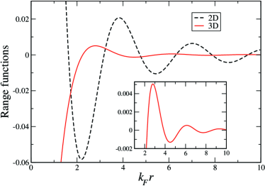
Figure 1: Comparison of the range functions for the RKKY interaction potentials in the 2D (black, dashed line) and 3D (red, solid line) spatial dimensions. The inset provides a magnified view of the 3D RKKY range function.

With an explicit form of the interaction in place [Eq. (12)], we are now in a position to take advantage of the random-field method that has initially been developed for bulk 3D samples [18, 19]. In this approach, any spin $S_{zj}$ is treated as a source of random field $H_{zi}\equiv\sum_{j\neq i}J(\mathbf{r}_{ij})S_{zj}$ which acts on other similar spins. Then, all observable properties of the system are determined by the distribution function $f(H)$ of the random field $H$. More precisely, any spin average $\overline{\langle A\rangle}$ has the form $\int A(H)f(H)dH$, where the bar stands for the averaging over the spatial disorder. In addition, $A(H)$ is a single-particle thermal average with an effective form of the Hamiltonian ${\cal H}$ [18, 19],

$${\cal H}_{\mathrm{eff}}=\sum_{i}H_{zi}S_{zi}.$$ (17)

The explicit expression for the distribution function $f(H)$ reads

$$f(H)=\left\langle\overline{\delta\left(H-\sum_{j(\neq i)}J(\mathbf{r}_{ij})S_{zj}\right)}\right\rangle.$$ (18)

As the configurational averaging (i.e., over the spatial disorder) and the thermal averaging cannot be achieved exactly in Eq. (18), we apply an alternative approach, i.e., the self-consistent averaging in the spirit of the statistical theory of magnetic resonance line shape [26]. By using the spectral representation of the $\delta$ function, a set of self-consistent equations can be obtained for the spin averages $m_{l}=(-1)^{l}~{}\overline{\langle S_{z}^{l}\rangle}$, $l=1,2,$… (analogous to the $l$-th order moment in a sense). The macroscopic magnetization $\mathcal{M}$ simply becomes $\mathcal{M}=g\mu_{B}m$ (with $m\equiv m_{1}$).

For an arbitrary spin $S$, the explicit form of this set reads [18, 19]

$$f(H)=\frac{1}{2\pi}\int_{-\infty}^{\infty}e^{iH\rho+\mathcal{G}(\rho)}d\rho,$$ (19a)

$$\mathcal{G}(\rho)=\left\langle\overline{n_{i}\int\left(e^{-iJ(\mathbf{r})\sigma\rho}-1\right)d^{2}r}\right\rangle$$

$$=\sum_{\sigma=1/2}^{S}\bigg{\{}a_{\sigma}\mathcal{F}_{0}(\sigma\rho)+ib_{\sigma}\mathcal{F}_{1}(\sigma\rho)\bigg{\}},$$ (19b)

$$a_{\sigma}+ib_{\sigma}=\int_{-\infty}^{\infty}\bigg{[}A_{\sigma}(h)+iB_{\sigma}(h)\bigg{]}f(H)dH,$$ (19c)

$$\mathcal{F}_{0}(z)+i\mathcal{F}_{1}(z)=n_{i}\int[\exp\left(iJ(\mathbf{r})z\right)-1]d^{2}r,$$ (19d)

$$A_{\sigma}(h)+iB_{\sigma}(h)=\frac{2}{Z_{S}}[\cosh(\sigma h)+i\sinh(\sigma h)],$$ (19e)

$$Z_{S}=\sum_{\sigma=-S}^{S}e^{-\sigma h}=\frac{\sinh[(S+1/2)h]}{\sinh(h/2)};h=\frac{H}{T}.$$ (19f)

The self-consistency is achieved by inserting Eq. (19a) into Eq. (19c) and integrating over $$H$$. This yields

$$a_{\sigma}+ib_{\sigma}=\int_{-\infty}^{\infty}\left[\mathcal{A}_{\sigma}(z)+i\mathcal{B}_{\sigma}(z)\right]$$

$$\times\exp\bigg{[}\sum_{\sigma=1/2}^{S}\bigg{\{}a_{\sigma}\mathcal{F}_{0}(z_{\sigma})+ib_{\sigma}\mathcal{F}_{1}(z_{\sigma})\bigg{\}}\bigg{]}dz,$$ (20a)

$$\mathcal{A}_{\sigma}(z)+i\mathcal{B}_{\sigma}(z)=\frac{1}{2\pi}\int_{-\infty}^{\infty}[A_{\sigma}(h)+iB_{\sigma}(h)]$$

$$\times\exp(izh)dh,\ z_{\sigma}=\frac{\sigma z}{T}.$$ (20b)

The above equations are valid for Ising spin of arbitrary magnitude $$S$$. Below we apply these equations to the representative case of spin 1/2 as well as S=5/2. A typical example is Mn ions which are ubiquitous magnetic impurities in 2D and 3D DMSs (see Refs. [8, 6, 14] and references therein).

For $S=1/2$, we have $\sigma=\pm 1/2$ and the governing equations result in the dimensionless magnetization

$$m=\int_{-\infty}^{\infty}\tanh\left(\frac{H}{2T}\right)f(H)dH,$$ (21)

where $f(H)$ is defined by Eq. (19a) with

$$\mathcal{G}(\rho) = \mathcal{F}_{0}\left(\frac{\rho}{2}\right)+i\mathcal{F}_{1}\left(\frac{\rho}{2}\right),$$ (22a)

$$\mathcal{F}_{0}\left(\frac{\rho}{2}\right) = 2\pi n_{i}\int_{0}^{\infty}\bigg{[}\cos\left(J(r)\frac{\rho}{2}\right)-1\bigg{]}rdr,$$ (22b)

$$\mathcal{F}_{1}\left(\frac{\rho}{2}\right) = 2\pi n_{i}\int_{0}^{\infty}\sin\left(J(r)\frac{\rho}{2}\right)\ rdr.$$ (22c)

Then, Eq. (21) assumes the form

$$m=T\int_{0}^{\infty}\frac{e^{\mathcal{F}_{0}(\rho)}}{\sinh\frac{\pi\rho T}{2}}\sin\left[m\mathcal{F}_{1}(\rho)\right]d\rho$$ (23)

following the integration over $H$ [19]. This expression defines the dimensionless magnetization $m$ in a self-consistent manner.

The MFA asymptotics of Eq. (23) corresponds to $n_{i}\rightarrow\infty$ [19], which reduces to $\rho\rightarrow 0$ as well as $\mathcal{F}_{0}(\rho)\rightarrow 0$. In this case, we can obtain from Eq. (23)

$$m = T\int_{0}^{\infty}\frac{\sin\left[m\rho W_{0}\right]}{\sinh\frac{\pi\rho T}{2}}d\rho,$$ (24)

$$W_{0} = 2\pi n_{i}\int_{0}^{\infty}rJ(r)dr\equiv T_{0}.$$ (25)

Here, $W_{0}$ actually corresponds to $T_{0}$ defined earlier in Eq. (8), which is the Curie temperature $T_{c}$ in the degenerate regime based on the so-called homogeneous Weiss field approximation [4]. This coincidence between the results of two different approaches is not accidental. It actually stems from the fact that the RKKY model implicitly takes into account the first-order contribution in the carrier-ion exchange coupling (i.e., the homogeneous Weiss field) along with the fluctuating second-order component to ensure the convergence of integral over the carrier wavevectors [17]. As such, the average over the RKKY oscillations [see the integration in Eq. (25)] cancels out the second-order term, leaving the contribution from the first-order intact.

Evaluation of the integral in Eq. (24) (i.e., the MFA asymptotics) yields, as expected, the well-known expression of the mean-field magnetization for the spin 1/2 Ising model

$$m=\tanh\frac{mT_{0}}{T}.$$ (26)

To obtain the phase-transition condition from Eq. (26), we apply the usual procedure $m\rightarrow 0$, which generates once more $T=T_{0}$. This procedure can be regarded as a consistency check for our approximation.

The same procedure $m\to 0$, when applied to the more accurate relation of Eq. (23), leads to the following random-field expression for $T_{c}$

$$1=T_{c}\int_{0}^{\infty}\frac{\mathcal{F}_{1}(\rho)e^{\mathcal{F}_{0}(\rho)}\ d\rho}{\sinh\frac{\pi\rho T_{c}}{2}}.$$ (27)

Contrary to the MFA shown in Eq.  (26), this relation indicates the existence of a critical condition associated with the case $T_{c}=0$. More specifically, at $T_{c}\to 0$, Eq. (27) can be reduced to

$$\frac{2}{\pi}\int_{0}^{\infty}\frac{\mathcal{F}_{1}(\rho)}{\rho}e^{\mathcal{F}_{0}(\rho)}\ d\rho=1.$$ (28)

The resulting condition is a complex function of $n_{i}$ and $n_{e}$ (thus, $\mu$). For a given host material and the magnetic ion density $n_{i}$, it specifies the free carrier concentration beyond which the long-range order is impossible in the system even at zero temperature.

The situation for $S=5/2$ is qualitatively the same, while the derivations are much more cumbersome. In fact, it is difficult even to write a closed form expression for the dimensionless magnetization. After some algebra, we arrive at the following equation for $T_{c}$

$$1 = \frac{2T_{c}}{7}\int_{0}^{\infty}\mathcal{F}_{11}(\rho)e^{\mathcal{F}_{01}(\rho)}L_{5/2}\left(\pi\rho T_{c}\right)d\rho,$$ (29a)

$$\mathcal{F}_{01}(\rho) = \frac{2\pi n_{i}}{3}\int_{0}^{\infty}\bigg{(}\cos\frac{5}{2}\zeta+\cos\frac{3}{2}\zeta+\cos\frac{1}{2}\zeta-3\bigg{)}rdr,$$

$$\mathcal{F}_{11}(\rho) = 2\pi n_{i}\int_{0}^{\infty}\bigg{(}\sin\frac{5}{2}\zeta+\frac{3}{5}\sin\frac{3}{2}\zeta+\frac{1}{5}\sin\frac{1}{2}\zeta\bigg{)}rdr,$$

$$\zeta = \rho J(r).$$ (29b)

Here $$L_{5/2}(z)=\coth\frac{z}{6}-\coth z L_{5/2}(z\rightarrow 0)=5/z$$. The expression for the critical concentration can be derived from Eq. (29a) via the asymptotic relation to yield

$$\frac{10}{7\pi}\int_{0}^{\infty}\frac{\mathcal{F}_{11}(\rho)}{\rho}e^{\mathcal{F}_{01}(\rho)}d\rho=1.$$ (30)

Equations (29a) and (30) are solved numerically in Sec. III.

III Results and Discussion

For the numerical calculation of the phase-transition temperature, it is convenient to express both $T_{c}$ and $\mu$ in units of $T_{0}$. In these units, Eq. (8) assumes the form

$$y\left(1+e^{-\frac{\xi_{0}}{y}}\right)=1,$$ (31)

where $y=T_{c}/T_{0}$ and $\xi_{0}=\mu/T_{0}$. Equation (31) indicates $y\to 1$ as $\xi_{0}\gg 1$; i.e., $T_{c}$ cannot exceed $T_{0}$. Furthermore, $T_{c}$ appears to attain its asymptotic value by $\mu\approx 5T_{0}$. Being based on the mean-field treatment, the dependence $y(\xi_{0})$ in Eq. (31) is expected to remain valid up to a moderately degenerate carrier gas in a 2D semiconducting host (obviously including the nondegenerate case). By contrast, Eq. (27) or (29a) can be used to describe $y(\xi_{0})$ for high values of $\xi_{0}$ (thus, $\mu$). Assuming magnetic ions Mn²⁺ with $S=5/2$ as an example, the numerical solution of Eq. (29a) similarly shows that $T_{c}\approx T_{0}$ at $\mu\approx 5T_{0}$ when approaching from the opposite, heavily degenerate regime. Thus, the chemical potential around $5T_{0}$ comprises the crossover between the two $n_{e}$ regimes, enabling the interpolation between them.

Figure 2 illustrates the combined outcome of $T_{c}$ vs. $\mu$ in the full range of $\mu$ (with $S=5/2$). Evidently, the maximal $T_{c}$ (or its close vicinity) can be achieved only in a relatively narrow range of $\mu$ near the crossover point. This is different from the mean-field model which predicts $T_{c}=T_{0}$ once $\mu$ becomes sufficiently large. As $\mu$ is lowered, $T_{c}$ shows a rather rapid but continuous decrease to a value $\approx 0.22T_{0}$ (denoted as $T_{c,tr}$) corresponding to $\mu_{min}\approx-0.28T_{0}$ and then the solution ceases to exist abruptly. This threshold behavior originates from the minimal density of free carriers needed to mediate the indirect exchange interaction. The latter restriction qualitatively distinguishes a 2D case from the 3D one, where $T_{c}^{3d}$ can be arbitrarily small but does not vanish even at an infinitesimal carrier density [27].

In the heavily degenerate regime, $T_{c}$ also reveals a gradual decrease but this time to zero. The $T_{c}=0$ condition from Eq. (30) gives the critical value $\mu_{cr}\approx 16.7T_{0}$. This decay to zero is because the averaging over the spatial disorder cancels out for $\mu\geq\mu_{cr}$ due to the rapid oscillations of the RKKY range function. In fact, the above observation reflects the fact that the ratio $\mu/T_{0}$ represents the geometric factor proportional to $(\bar{R}/\bar{r})^{2}$, where $\bar{R}$ ($\sim n_{i}^{-1/2}$) is a mean distance between magnetic ions and $\bar{r}$ ($\sim k_{F}^{-1}\sim\mu^{-1/2}$) approximates the RKKY oscillation period shown in Fig. 1. Interestingly, its inverse $(\bar{r}/\bar{R})^{2}$ can be interpreted as the mean number of magnetic ions interacting coherently with each other by the dominant FM spin-spin coupling. As increasing $\mu$ reduces $\bar{r}$ and the number of ions interacting coherently, the FM order becomes unsustainable beyond a certain critical value (i.e., $\mu_{cr}$). Combined with the analysis in the non-/weakly degenerate regime discussed earlier, our model predicts that the FM ordering can be achieved only for $\mu_{min}<\mu<\mu_{cr}$ with the optimum condition around $5T_{0}$.

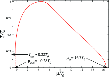
Figure 2: FM phase-transition temperature $T_{c}$ vs. the chemical potential $\mu$ (both in units of $T_{0}$) in a 2D DMS with $S=5/2$. The abscissa axis also corresponds to a ratio between the free-carrier and magnetic ion densities $n_{e}$ and $n_{i}$ (except a constant). In the mean-field treatment, $T_{c}$ would stay at $T_{0}$ with no dependence on $\mu$ in the highly degenerate regime. The dashed line projects the condition at which the FM ordering ceases to exist in the nondegenerate regime.

Note that the overall behavior of $T_{c}(\mu)$ for $\mu\gtrsim 5T_{0}$ appears similar to that in 3D bulk samples [18]. This is to be expected judging from the comparable characteristics of the RKKY range functions (except the magnitude) described in Fig. 1. The only difference is the exact form of the normalization factor $T_{0}$ which shows disparate functional dependences in the 2D and 3D cases. On the other hand, this very difference in $T_{0}$ illustrates a distinct feature of the 2D system in the non-/weakly degenerate regime. As the curve $T_{c}(\mu)$ in the bulk samples has shown qualitative accord with the experiments and Monte Carlo simulations in the degenerate regime [28], it is reasonable to anticipate a similar level of agreement in the 2D structures under consideration. Of course, it should be noted that the current 2D model is limited by consideration of Ising impurity spins as described above.

For numerical estimation of $T_{c}$ in a realistic case, a QW of Cd_0.9Mn_0.1Te is chosen as a specific example. The values of the relevant parameters found in the literature [29] are the carrier-ion exchange constant $I=0.88$ eV and the hole effective mass $m^{\ast}=0.8m_{0}$, where $m_{0}$ is the free electron mass. In addition, the 2D hole density $n_{e}$ is estimated to be $\approx 10^{11}$ cm^-2 that leads to $\mu/T_{0}\cong 8$ at $x_{i}=10\%$. Substituting all these values to the expression predicts $T_{c}\approx 180$ K, which is a high value for a DMS. This analysis further suggests that $T_{c}$ can be increased by another 30 % or so (to $\sim 240$ K) if the free hole density is lowered (not raised contrary to the conventional perception) by about 40 % to the desired $\mu/T_{0}\approx 5$. Controlling $n_{e}$ (thus, $\mu$) independent of $n_{i}$ is clearly possible, which is particularly so in the 2D structures. Note that our estimation of $T_{c}$ is rather rough as the values of the material parameters are temperature, pressure and other external stimuli dependent. Nevertheless, the results strongly indicate that the FM ordering can be achieved even at/above room temperature when the 2D DMS systems are properly optimized. For instance, recent ab initio calculations predicted the carrier-ion exchange constant significantly larger than 1 eV in magnetically doped 2D transition-metal dichalcogenides along with comparable hole effective masses [30, 31]. Hence, it is not unreasonable to expect a substantial enhancement of $T_{c}$ in these structures, where the modulation of free carrier concentrations over a wide range can be readily achieved [32].

IV Summary and Outlook

Possible magnetic long-range order in the doped planar semiconductor structures with Ising impurity spins exhibits a large body of interesting physical effects, making them promising candidates for spintronic, electronic and even photovoltaic applications [1, 3, 33]. In this work, we demonstrate that the magnetic impurities, realizing the Friedel oscillations of the constituent 2D free carrier gas, may generate room temperature FM order in a host structure. The conditions suitable to reach the maximum possible $T_{c}$ is elucidated, which can provide a useful guideline for experimental realization. It is noted that the onset of ferromagnetism considered here is due only to the RKKY interaction, while there are evidently other mechanisms (like direct ferro- or antiferromagnetic exchange between the close pairs of impurities) that can also promote the appearance of magnetic order in the 2D semiconductor structures [15, 16, 14]. Further, there is another important effect which is present in all 2D structures except graphene. This effect is related to the synergy between the RKKY indirect exchange coupling and the Rashba spin-orbit interaction, leading to the interesting phenomena such as the strong anisotropy in the resulting $J(r)$ [34]. These and other higher-order effects are outside the scope of the current study.

- [1] I. Žutić, J. Fabian, and S. Das Sarma, ”Spintronics: Fundamentals and applications,” Rev. Mod. Phys. 76, 323 (2004).
- [2] E. I. Rashba, ”Spintronics: Sources and Challenge. Personal Perspective,” J. Supercond. 15, 13 (2002).
- [3] M. Bibes, J. E. Villegas, and A. Barthélémy, ”Ultrathin oxide films and interfaces for electronics and spintronics,” Adv. Phys. 60, 5 (2011).
- [4] W. A. Harrison, Solid State Theory (Dover, New York, 1979).
- [5] J. M. Ziman, Principles of the Theory of Solids (Cambridge University Press, Cambridge, 1979).
- [6] W. Choi, N. Choudhary, G. H. Han, J. Park, D. Akinwande, and Y. H. Lee, ”Recent development of two-dimensional transition metal dichalcogenides and their applications,” Mater. Today 20, 116 (2017).
- [7] A. Kirilyuk, A. V. Kimel, and T. Rasing, ”Ultrafast optical manipulation of magnetic order,” Rev. Mod. Phys. 82, 2731 (2010).
- [8] S. Manzeli, D. Ovchinnikov, D. Pasquier, O. V. Yazyev, and A. Kis, ”2D transition metal dichalcogenides,” Nat. Rev. Mater. 2, 17033 (2017).
- [9] M. V. Costache, M. Sladkov, S. M. Watts, C. H. van der Wal, and B. J. van Wees, ”Electrical detection of spin pumping due to the precessing magnetization of a single ferromagnet,” Phys. Rev. Lett. 97, 216603 (2006).
- [10] L. D. Landau and E. M. Lifshitz, ”On the theory of the dispersion of magnetic permeability in ferromagnetic bodies,” Phys. Z. Sowjetunion 8, 153 (1935).
- [11] T. L. Gilbert, ”A phenomenological theory of damping in ferromagnetic materials,” IEEE Trans. Magn. 40, 3443 (2004).
- [12] E. A. Pashitskij and S. M. Ryabchenko, ”Magnetic ordering in semiconductors with magnetic impurities,” Fiz. Tverd. Tela (Leningrad), 21, 545 (1979) [Sov. Phys. Solid State 21, 322 (1979)].
- [13] T. Dietl, H. Ohno, and F. Matsukura, ”Hole-mediated ferromagnetism in tetrahedrally coordinated semiconductors,” Phys. Rev. B 63, 195205 (2001).
- [14] T. Dietl and H. Ohno, ”Dilute ferromagnetic semiconductors: Physics and spintronic structures,” Rev. Mod. Phys. 86, 187 (2014).
- [15] Introduction to the physics of diluted magnetic semiconductors, eds. J. Kossut and J. A. Gaj (Springer, New York, 2010).
- [16] J. Cibert and D. Scalbert, ”Diluted magnetic semiconductors: Basic physics and optical properties,” in Spin Physics in Semiconductors, ed. M. I. Dyakonov (Springer Series in Solid-State Sciences, vol 157. Springer, Berlin, Heidelberg, 2008).
- [17] Y. G. Semenov, S. M. Ryabchenko. ”Molecular-field approximations in the theory of ferromagnetic phase transition in diluted magnetic semiconductors,” Ukr. J. Phys. 66, 503 (2021).
- [18] Yu. G. Semenov and V. A. Stephanovich, ”Suppression of carrier-induced ferromagnetism by composition and spin fluctuations in diluted magnetic semiconductors,” Phys. Rev. B 66, 075202 (2002).
- [19] Y. G. Semenov and V. A. Stephanovich, ”Enhancement of ferromagnetism in uniaxially stressed dilute magnetic semiconductors,” Phys. Rev. B 67 195203 (2003).
- [20] S. M. Ryabchenko, Y. G. Semenov, A. V. Komarov, T. Wojtowicz, G. Cywinski, and J. Kossut, ”Optical polarization anisotropy of quantum wells induced by a cubic anisotropy of the host material,” Physica E 13 , 24 (2002).
- [21] C. Kittel, Quantum Theory of Solids (John Wiley and Sons, New York, 1987).
- [22] M. Abolfath, T. Jungwirth, J. Brum, and A. H. MacDonald, ”Theory of magnetic anisotropy in III1-xMnxV ferromagnets,” Phys. Rev. B 63, 054418 (2001).
- [23] V. I. Litvinov and V. K. Dugaev, ”RKKY interaction in one- and two-dimensional electron gases,” Phys. Rev. B 58, 3584 (1998).
- [24] M. T. Béal-Monod, ”Ruderman-Kittel-Kasuya-Yosida indirect interaction in two dimensions,” Phys. Rev. B 36, 8835 (1987).
- [25] Handbook of Mathematical Functions, eds. M. Abramowitz and I. I. Stegun (Dover, New York, 1972).
- [26] A. M. Stoneham, ”Shapes of inhomogeneously broadened resonance lines in solids,” Rev. Mod. Phys. 41, 82 (1969).
- [27] Y. G. Semenov and S. M. Ryabchenko, ”Exactly solvable model for carrier-induced paramagnetic-ferromagnetic phase transition in diluted magnetic semiconductors”, Physica E 10 , 165 (2001).
- [28] D. Ferrand, J. Cibert, A. Wasiela, C. Bourgognon, S. Tatarenko, G. Fishman, T. Andrearczyk, J. Jaroszyński, S. Koleśnik, T. Dietl, B. Barbara, and D. Dufeu, ”Carrier-induced ferromagnetism in p-Zn1-xMnxTe,” Phys. Rev. B 63, 085201 (2001).
- [29] T. Dietl, A. Haury, and Y. Merle d’Aubigné, ”Free carrier-induced ferromagnetism in structures of diluted magnetic semiconductors,” Phys. Rev. B 55, R3347 (1997).
- [30] M. Pan, J. T. Mullen, and K. W. Kim, ”First-principles analysis of magnetically doped transition-metal dichalcogenides,” J. Phys. D: Appl. Phys. 54, 025002 (2021).
- [31] Z. Jin, X. Li, J. T. Mullen, and K. W. Kim, ”Intrinsic transport properties of electrons and holes in monolayer transition metal dichalcogenides,” Phys. Rev. B 90, 045422 (2014).
- [32] B. Radisavljevic, A. Radenovic, J. Brivio, V. Giacometti, and A. Kis, ”Single-layer MoS2 transistors,” Nat. Nanotechnol. 6, 147 (2011).
- [33] S. D. Stranks and H. J. Snaith, ”Metal-halide perovskites for photovoltaic and light-emitting devices,” Nat. Nanotechnol. 10, 391 (2015).
- [34] H. Imamura, P. Bruno, and Y. Utsumi, ”Twisted exchange interaction between localized spins embedded in a one- or two-dimensional electron gas with Rashba spin-orbit coupling,” Phys. Rev. B 69, 121303(R) (2004).