Effects of the growth kinetics on solute diffusion in porous films

Abstract

For the development of porous materials with improved transport properties, a key ingredient is to determine the relations between growth kinetics, structure, and transport parameters. Here we address these relations by studying solute diffusion through three-dimensional porous films produced by deposition models with controlled thickness and porosity. A competition between pore formation by lateral particle aggregation and surface relaxation that favors compaction is simulated by the lattice models of ballistic deposition and of random deposition with surface relaxation, respectively, with relative rates proportional to $p$ and $1-p$. Effective diffusion coefficients are determined in steady state simulations with a solute source at the basis and a drain at the top outer surface of the films. For a given film thickness, the increase of the relative rate of lateral aggregation leads to the increase of the effective porosity and of the diffusivity, while the tortuosity decreases. With constant growth conditions, the increase of the film thickness always leads to the increase of the effective porosity, but a nontrivial behavior of the diffusivity is observed. For deposition with $p\leq 0.7$, in which the porosity is below $0.6$, the diffusion coefficient is larger in thicker films; the decrease of the tortuosity with the thickness quantitatively confirms that the growth continuously improves the pore structure for the diffusion. Microscopically, this result is associated with narrower distributions of the local solute current at higher points of the deposits. For deposition with $p\geq 0.9$, in which the films are in the narrow porosity range $\sim 0.65-0.7$, the tortuosity is between $1.3$ and $2$, increases with the thickness, and has maximal changes near $25\%$. Pairs of values of porosity and tortuosity obtained in some porous electrodes are close to the pairs obtained here in the thickest films, which suggests that our results may be applied to deposition of materials of technological interest. Noteworthy, the increase of the film thickness is generally favorable for diffusion in their pores, and the exceptions have small losses in tortuosity.

1 Introduction

The development of porous materials with improved transport properties is interesting for several technological applications, such as electrodes in energy storage devices ¹, ², membranes for ion or molecule separation ³, ⁴, and catalysis ⁵, ⁶. For instance, the design of high capacity Li-ion batteries partly relies on the production of porous electrodes that are mechanically stable and offer low resistance to electron and ion transport ⁷. This may be achieved with better battery designs or with the development of novel materials. In all cases, it is important to understand the relation between the conditions in which the materials are formed, the geometry of their porous systems, and transport parameters such as conductivities or diffusion coefficients. Since electrodes are frequently produced in the form of thin films, it is reasonable to search for those relations in this type of structure.

Several works have already addressed the relations between structural and transport properties in porous media, with interest not only on manufactured materials but also in natural ones such as rocks and soils ⁸, ⁹. In most cases, the porous media are modeled with preset distributions of solid and pore space, such as regular or random sphere packings ¹⁰, ¹¹, ¹², fiber networks ¹³, tubes with cage-throat geometry ⁵, ¹⁴, etc, or use reconstructed images of the materials of interest ¹⁵, ¹⁶. Recent works modeled porous electrodes and performed transport simulations using several methods ¹⁷, ¹⁸, ¹⁹, ²⁰. However, they do not account for the dynamical processes for porous media formation.

Here we advance in the determination of structure-transport relationships by studying models that connect them with the conditions of film growth. We study diffusional transport of a solute through films with broad ranges of porosity and thickness, which are formed by sequential aggregation of particles that may follow mechanisms of pore formation or of surface relaxation. Tuning the relative rate of these mechanisms changes the growth kinetics and, consequently, changes bulk and surface properties. Besides analyzing the effects of changing growth conditions, we also investigate the effects of film thickness and surface roughness on quantities such as porosity and tortuosity. Among the results, we highlight the observation that the increase of the thickness is beneficial for the diffusivity in all films with porosity below $60\%$, with tortuosity reductions reaching factors close to $5$ when the porosity is near $20\%$. The relations between porosity and tortuosity obtained here closely match the relations obtained in some porous electrodes, which suggests that our results may be relevant for their production.

The competitive growth kinetics is simulated in three dimensions (3D) with two widely studied models: ballistic deposition (BD) ²¹, ²², in which pores are formed by lateral aggregation of particles, and random deposition with surface relaxation (RDSR) ²³, which favors the formation of compact structures. The competitive BD-RDSR model can describe a variety of conditions for formation of porous films, with the constraints of an at least partially collimated particle flux and of negligible subsurface relaxation. These mechanisms differ, for instance, from those of evaporation-induced nanoparticle assembly, which were recently modeled in two dimensions (2D) ²⁴, and from deposition with flux distributed in several directions ²⁵.

The rest of this paper is organized as follows. In Sec. 2, we present the deposition model, the model of diffusive transport, the quantities of interest, and a brief review of previous results on the BD-RDSR model. In Sec. 3, we show numerical results for the structural properties of the deposits, the effective diffusion coefficients in their pores, and the distributions of local solute currents in their cross sections. In Sec. 4, we analyze the relations between the growth conditions, the film structure, and the transport parameters. In Sec. 5, we summarize our results and present our conclusions. A list of symbols used in this paper is presented in Table LABEL:NomenclatureTable.

2 Model and methods

2.1 Film deposition

The deposit has simple cubic lattice structure with sites of edge length $a$. Deposition occurs on a flat substrate located at $z=0$, with lateral size $L$, and periodic boundary conditions in $x$ and $y$ directions. Each deposited particle occupies one lattice site. Depending on the application of the model, a particle may represent a molecule, an aggregate, or a nanoparticle. The set of particles with the same $\left(x,y\right)$ positions is termed a column of the deposit. The height $h\left(x,y\right)$ is the maximal height $z$ of a particle in a column and the set $\{h\left(x,y\right)\}$ defines the top outer surface.

Incident particles are sequentially released in randomly chosen columns $(x,y)$, with $z$ larger than all $h\left(x,y\right)$, and follow a trajectory in the $-z$ direction. The rules for their aggregation are illustrated in Fig. 1. With probability $p$, the particle aggregates according to the BD rule, namely at its first contact with a previously deposited nearest neighbor (NN) ²², ²¹. The aggregation in a lateral contact (e.g. at the left in Fig. 1) either creates a pore or expands an existing pore. With probability $1-p$, the incident particle follows the RDSR rule: it attaches at the top of the column of incidence if no NN column has a smaller height, otherwise it moves to the top of the NN column with the minimal height; in the case of a draw, one of the columns with minimal height is randomly chosen ²³. The aggregation follows the same rules when the particle is adsorbed on the substrate and in the deposit.

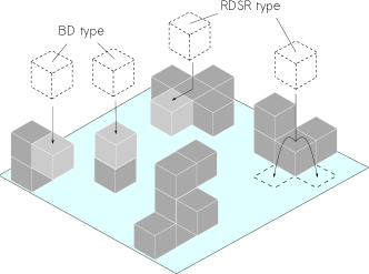
Figure 1: Scheme of the aggregation mechanisms of BD and RDSR. Dashed cubes are incoming particles, dark gray cubes are aggregated particles, and light gray cubes show the aggregation position of some incoming particles. If more than one aggregation position can be chosen, they are indicated by the split arrows.

Figs. 2(a)-(c) show horizontal cross sections and small 3D parts of the deposits produced with some values of $p$. Close inspection indicates that the porosity and the connectivity increase with $p$. Details of the simulations of film growth and calculation of structural properties are in Sec. SI.I of the Supporting Information.

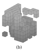
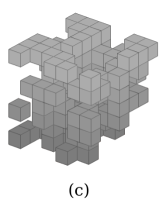
Figure 2: Horizontal cross sections and small parts of the 3D deposits grown with (a) $p=0.4$, (b) $0.7$, and (c) $1$.

The BD-RDSR model is not intended to describe a particular deposition process, but it is designed to be an approximation of thin film deposition processes with competitive adsorption mechanisms. This competition is simplified by aggregation at first contact, with relative rate $p$, and surface relaxation, with relative rate $1-p$. For instance, in some sputtering processes, the energy distribution of ions, molecules, or clusters may be broad, so that the aggregation at the first contact is more likely for the species with low energy, while those with high energy tend to form locally compact configurations. In this case, the energy distribution depends on the interactions of ions and the target source. Similar interpretation is possible in electrospray deposited films if there are differences in the nanoparticle aggregation rates due to charge distributions. In cases of deposition of a mixture with a binder, the concentration of this binder may control the rate of pore formation; this is done in the production of battery electrodes. Thus, it is frequently possible to infer which changes in the growth conditions will increase or decrease the effective value of $p$, although it is difficult to estimate that value directly from the growth parameters (this estimation may be done by comparing the structural properties that are calculated here). Another important feature of the BD-RDSR model is to describe short range surface relaxation processes, i.e. relaxation only to NNs. This is expected to be a reasonable approximation for low temperatures and high deposition fluxes, in which adsorbed particles or aggregates have small surface mobility.

When $N_{d}$ is the number of deposited particles, the dimensionless growth time is defined as the number of particles per column, $t_{g}=N_{d}/{\left(L/a\right)}^{2}$.

2.2 Structural properties

The dimensionless thickness $H$ is the average of the dimensionless heights $\{h/a\}$ of the top outer surface:

$$H=\left\langle\frac{1}{{\left(L/a\right)}^{2}}\sum_{x,y}{\frac{h\left(x,y\right)}{a}}\right\rangle,$$ (1)

where the angular brackets denote an average over different deposits with the same growth time $t_{g}$. Fluctuations of the outer surface profile are quantified by the dimensionless roughness

$$W=\Bigg{\langle}\sqrt{\frac{1}{\left(L/a\right)^{2}}\sum_{x,y}{\left[\frac{h\left(x,y\right)}{a}-H\right]^{2}}}\Bigg{\rangle}.$$ (2)

The deposit is limited by five flat surfaces, namely the substrate and the four lateral sides, and the top outer surface, so its total volume is $V_{T}=L^{2}Ha$. The total porosity $\epsilon_{T}$ is defined as the pore volume fraction:

$$\epsilon_{T}=1-\frac{N_{d}a^{3}}{V_{T}}=1-\frac{t_{g}}{H}=1-\frac{1}{v_{a}},$$ (3)

where $v_{a}=H/t_{g}$ is a dimensionless growth velocity averaged over the total growth time.

The effective porosity or connected porosity $\epsilon_{E}$ is the volume fraction that can be filled by a fluid or a solute transported through the porous medium. Here, the substrate is the frontier where the solute flows in, with a source below it, and the top outer surface is the frontier where the solute flows out, with the drain specified as $\{z(x,y)\textrm{ }|\textrm{ }z>h(x,y),\textrm{ }\forall\textrm{ }(x,y)\}$. Fig. 3 shows a 2D porous deposit and indicates the two frontiers, the source, and the drain (this facilitates visualization in comparison with 3D images). We also assume that two pores are connected if they are NN and define the connected pore system as the set of internal pores that are connected to both frontiers by some sequence of NN internal pores; this system is also indicated in Fig. 3. Denoting its volume as $V_{c}$, the effective porosity is

$$\epsilon_{E}\equiv\frac{V_{c}}{V_{T}}.$$ (4)

Isolated pores are those that do not belong to the connected pore system.

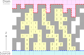
Figure 3: Sketch of a two-dimensional film with solid particles (gray), a connected pore system (yellow), and unconnected pores (white). The black dash-dotted line indicates the frontier of the source (blue) and the red dash-dotted line indicates the frontier of the drain (rose). Connected porous domains are labeled with numbers.

A connected domain of the pore system is defined by: $(i)$ it is a pore set connected to both frontiers; $(ii)$ all pairs of sites in the domain are also connected by a sequence of NN pores of that domain. Fig. 3 shows three connected domains in a 2D deposit. The average number of connected domains is used here to quantify the film structure. Their enumeration and the calculation of $\epsilon_{E}$ were performed via a 3D version of the Hoshen-Kopelman algorithm ¹, ⁵.

2.3 Transport simulations

We simulate solute transport across the deposits after the growth has stopped, using an extension of an infiltration model ²⁸. The concentration $C$ in a pore site or in the source is discretized, with possible values $0$ (empty) and $1$ (occupied). For applications in which the pore volume may contain more than one molecule, the local solute concentration has to be determined by averaging the occupation number over a larger volume.

A constant value $C=1$ is set at the source and $C=0$ is set at the drain. The molecules in the pore system and in the source execute random walks to NN sites with a rate $\nu$, which is defined as the number of hop attempts per unit time. Hop attempts to occupied pores or to solid sites are rejected and the molecule remains at its current position. When a molecule leaves the source, another molecule is immediatly inserted at its previous position, and when a molecule crosses the top frontier, it is removed from the system; this maintains the concentrations in the source and in the drain. In the hydrodynamic limit, the average concentration obeys the diffusion equation with the same boundary conditions ²⁹.

Figs. 4(a) and 4(b) show 2D schemes of the model in a free medium and in a porous deposit, respectively.

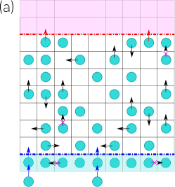
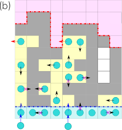
Figure 4: Two-dimensional illustration of the transport of solute molecules (circles) (a) in a free medium and (b) in the pores of a deposit, using the same color scheme of Fig. 3. Periodic conditions in the lateral boundaries are considered. The arrows indicate hop attempts of some molecules and the rejected attempts have arrows overlayed with a cross. Particles that reach the drain are removed from the system (red arrows) and particles that hop from the source to a pore are immediately replaced (blue arrows).

The currents $J_{in}$ and $J_{out}$ are defined as the average numbers of molecules that cross the frontiers per unit time of infiltration (this time does not include the growth time $t_{g}$). After a transient, solute transport reaches a steady state, in which these currents fluctuate around a constant value. The stationary current $J_{s}$ is calculated by averaging them in time and over different deposits. The effective diffusion coefficient $D_{E}$ of the solute is expressed in terms of the coefficient $D_{0}$ in the free medium as

$$D_{r}=\frac{D_{E}}{D_{0}}=6\left(H+1\right)\frac{J_{s}a^{2}}{\nu},$$ (5)

where $H+1$ stands for the average distance between the frontiers (see Fig. 3) and $D_{r}$ is a normalized or relative effective diffusion coefficient. Details on the method are in Sec. SI.II of the Supporting Information.

We also calculated the time-averaged solute concentrations $\overline{C}\left(x,y,z\right)$ in the steady states of some deposits and use them to determine the average solute current $\vec{j}_{s}$ as

$$\vec{j}_{s}=-a^{2}\nu\vec{\nabla}{\left(\frac{\overline{C}}{a^{3}}\right)}$$ (6)

(note that $C$ was defined as a dimensionless concentration). A dimensionless local current is defined as $\vec{j}=\left(a^{2}/\nu\right)\vec{j}_{s}$; distributions of its absolute value, $j(x,y,z)$, and of its $z$ component, $j_{z}(x,y,z)$, are used to analyze local transport properties.

2.4 Previous results on the BD-RDSR model

As a film grows in a wide substrate, the roughness is frequently observed to increase as a power law in time: $W\sim t_{g}^{\beta}$, where $\beta$ is the growth exponent ²¹, ³⁰. Surface fluctuations in the BD model are described in the hydrodynamic limit by the Kardar-Parisi-Zhang (KPZ) equation ³¹. All 3D models in the KPZ class have $\beta\approx 0.243$ ³². However, in simulations of BD and in other models with lateral particle aggregation, the average slopes of $\log{W}\times\log{t_{g}}$ plots are usually smaller than $\beta$ for $t_{g}\lesssim{10}^{5}$. This is ascribed to an intrinsic roughness $\xi_{I}$ that affects the roughness scaling as $W^{2}\simeq\xi_{I}+At_{g}^{2\beta}$ ($A$ constant) ³³, ³⁴.

The instantaneous growth velocity $v_{g}={\text{d}}H/{\text{d}}t_{g}$ in KPZ models varies in time as ³⁵

$$v_{g}=v_{\infty}-\Lambda{t_{g}}^{-\alpha_{\bot}},$$ (7)

where $\alpha_{\bot}=1-\beta\approx 0.76$ in 3D, and $v_{\infty}$ and $\Lambda$ are constants. In porous film growth, $\Lambda>0$, so the growth velocity slowly increases in time.

Surface fluctuations of the RDSR model are described by the Edwards-Wilkinson (EW) equation ³⁶, ²¹, which implies that the roughness scales as $W^{2}\sim\ln{t_{g}}$. No previous work on RDSR has shown large corrections to this scaling relation.

The BD-RDSR model was proposed to study a roughening transition between the EW and the KPZ classes ³⁷. Nonperturbative renormalization group calculations discards such transition in 3D ³⁸, which implies that the model is in the KPZ class for all $p>0$. However, deviations may be observed in simulations due to e.g. the intrinsic roughness. In BD-RDSR in 2D, long crossovers from EW to KPZ scaling were already shown for small $p$ ³⁹, ⁴⁰, ⁴¹.

Bulk properties of BD-RDSR deposits in 2D were formerly investigated ⁴², but no connected pore system emerges in this case; inspection of images of ballistic deposits in 2D actually show that $\epsilon_{E}=0$ ²¹, ⁴³. However, BD-RDSR deposits in 3D show a transition in the percolation class ⁵ at $p_{c}\approx 0.35$, i.e. there is a connected pore system for $p>p_{c}$ and there is no such system for $p<p_{c}$ ². This motivates the present study of films grown above $p_{c}$ as controlled templates for porous media with $\epsilon_{E}>0$. Diffusion of adsorbed molecules was already studied in the pore walls of 3D films grown by BD ($p=1$) ⁴⁵, but the study was constrained to transient regimes. To our knowledge, no previous work has studied the coupling of structural and transport properties in BD-RDSR films.

3 Results

3.1 Film thickness and surface roughness

The instantaneous velocity has slow variation in time, as predicted in Eq. (7). Thus, at long times, the average thickness $H$ has an approximately linear increase with $t_{g}$. Details are shown in Sec. SI.III of the Supporting Information.

Fig. 5 shows the time evolution of the roughness for several $p$. At a fixed growth time $t_{g}$, the roughness increases with $p$, which is expected because BD produces rougher deposits than RDSR. The same is observed for a fixed thickness $H$. The slope of the plots for $p\approx 1$ are near $0.14$, which differs from the KPZ value; this can be related to the intrinsic width correction discussed in Sec. 2.4. However, as the BD aggregation is less frequent ($p\approx 0.4$), the average slope becomes closer to the KPZ value $\beta\approx 0.24$.

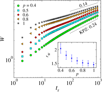
Figure 5: Roughness as function of the growth time for several values of $p$. Dashed lines have the indicated slopes. The inset shows the ratio $r_{W}$ as function of $p$. The uncertainties are smaller than the size of the symbols in all plots.

To relate structural film properties, we analyze the variation of the roughness with the thickness. For constant growth conditions, i.e. constant $p$, we calculate the ratio $r_{W}$ between the roughness of relatively thick films, with $H=10^{3}$, and of relatively thin films, with $H=50$: $r_{W}=W\left(H={10}^{3}\right)/W\left(H=50\right)$. The inset of Fig. 5 shows $r_{W}$ as a function of $p$. The films with smoother surfaces, which are produced with $p\approx 0.4$, have a faster increase in the roughness with the thickness (i.e. larger $r_{W}$) in comparison with the rougher films produced with $p\approx 1$.

3.2 Porosity and connectivity

We begin with a brief review of the results of BD-RDSR in 2D ⁴². For a fixed growth time or fixed thickness, the total porosity $\epsilon_{T}$ increases with $p$, which is expected because lateral aggregation facilitates the formation of pores. For constant $p$, Eqs. (3) and the KPZ relation (7) for the growth velocity explain why $\epsilon_{T}$ slowly increases with the thickness (the evolution of the average velocity $v_{a}$ is similar to that of the instantaneous velocity $v_{g}$). However, all deposits in 2D have effective porosity $\epsilon_{E}=0$. Thus, $\epsilon_{E}$ cannot be predicted from known relations of KPZ scaling and have to be determined numerically.

In 3D, for constant $p$, we also observe the expected increase of $\epsilon_{T}$ with the thickness. Fig. 6(a) shows the same evolution for the numerically calculated estimates of $\epsilon_{E}$ in cases where a connected pore system is formed, i.e. $p>p_{c}\approx 0.35$; for $p<p_{c}$, $\epsilon_{E}=0$ ².

The inset of Fig. 6(a) shows the relative difference between the total and the effective porosities, $\Delta_{\epsilon}=\left(\epsilon_{T}-\epsilon_{E}\right)/\epsilon_{T}$, which measures the fraction of the pore volume that cannot participate in the transport. For $p\geq 0.7$ and $H>20$, this difference is small ($\lesssim 2\%$), which means that isolated pores are seldom formed. In the less porous films ($p=0.4-0.6$), non-negligible values of $\Delta_{\epsilon}$ persist in large thicknesses.

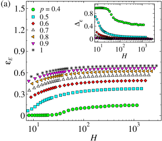
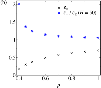
Figure 6: (a) Effective porosity as function of the film thickness for several values of $p$. The inset shows the relative difference between total and effective porosities. (b) Effective porosity of very thick ($H\gtrsim 10^{4}$) films (crosses) and the ratio $r_{\epsilon}$ (asterisks) as function of $p$. The uncertainties are smaller than the sizes of the symbols in all plots.

$\epsilon_{E}$ has a nontrivial evolution for small thicknesses; see Fig. 6(a). After these transients, the slow variation allows us to extrapolate $\epsilon_{E}$ to the limit $H\to\infty$; see details in Sec. SI.IV of the Supporting Information. For each $p$, this extrapolation gives an effective porosity $\epsilon_{\infty}$, which is representative of films with $H\gtrsim{10}^{4}$ with an accuracy $\approx 1\%$; this is hereafter termed thick film limit. Fig. 6(b) shows that $\epsilon_{\infty}$ also increases with $p$, extending the previous observations to much thicker films.

We also calculated the ratio $r_{\epsilon}=\epsilon_{\infty}/\epsilon_{E}\left(H=50\right)$, which quantifies the relative increase in the porosity from thin film conditions ($H=50$) to the thick film limit. This ratio is also shown in Fig. 6(b). The films with larger porosities are those that have slower variations in the porosity with the thickness, i.e. have $r_{\epsilon}\approx 1$. Instead, the films with relatively smaller porosity show faster variations with the thickness; for instance, the porosity of films grown with $p=0.4$ increase more than $100\%$ from $H=50$ to the thick film limit.

The evolution of the numbers of connected domains is shown in Sec. SI.V of the Supporting Information. For $p\geq 0.5$, a single connected domain is found in thickness $H\approx 20$ or larger; for $p=0.4$, it occurs in $H\geq 60$. Thus, in all samples, there is a progressive merging of multiple percolating domains into a single, large percolating pore cluster.

3.3 Diffusion coefficients

Fig. 7(a) shows the normalized diffusion coefficient $D_{r}$ as a function of the film thickness for $p\leq 0.7$; Fig. 7(b) shows the same quantities for $p>0.7$. In contrast with the structural quantities, the evolution of $D_{r}$ shows different trends: for $p<0.8$, $D_{r}$ increases with the thickness (the same as $\epsilon_{E}$); for $p>0.8$, $D_{r}$ decreases with the thickness (the opposite of $\epsilon_{E}$).

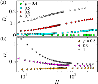
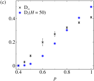
Figure 7: (a),(b): Normalized diffusion coefficient as function of film thickness for small and large values of $p$, respectively. (c) Normalized diffusion coefficients of very thick films, $D_{\infty}$, and of thin films with $H=50$, $D_{r}\left(H=50\right)$, as a function of $p$. Error bars of $D_{\infty}$ are shown, but uncertainties in the other estimates are smaller than the sizes of the symbols.

The variations of $D_{r}$ also suggest to compare results in thin and thick films. The effective diffusion coefficient in the thick film limit, $D_{\infty}$, is estimated using the same method adopted to calculate $\epsilon_{\infty}$; see Sec. SI.IV of the Supporting Information. $D_{\infty}$ is also a good approximation for the normalized diffusion coefficient in all films with $H\gtrsim{10}^{4}$. Fig. 7(c) shows $D_{\infty}$ and the normalized diffusion coefficient in relatively thin films, $D_{r}\left(H=50\right)$, as a function of $p$. It confirms the nontrivial behavior for $p\geq 0.9$, in which the diffusivity decreases with the thickness; these films have porosity between $0.6$ and $0.7$ for all thicknesses $H\geq 50$. Instead, in films grown with $p\leq 0.7$, which have $\phi_{E}<0.6$ for all thicknesses, the diffusivity increases with the thickness.

These different trends are balanced near $p=0.8$, in which $\phi_{E}\approx 0.6$ and $D_{r}\approx 0.3$. The exact value $p^{*}$ in which this balance occurs depends on the choice of the thickness to be compared with the thick film limit; for instance, if $H=50$ is chosen, the balance is estimated to occur at $p^{*}=0.84$.

3.4 Distributions of local solute currents

Figs. 8(a) and 8(b) show configurations of the absolute value of the local solute current in vertical cross sections of films with thicknesses $\sim 200$ grown with $p=0.6$ and $p=1$, respectively. Figs. 8(c)-(f) show configurations in horizontal cross sections of the same films at different heights. In films grown with $p=0.6$, the density of spots of large current ($j\gtrsim 0.005$; reddish color) decreases as $z$ increases, while spots of intermediate current ($0.002\leq j\leq 0.003$) become dominant at $z=100$. The opposite trend is observed in the films grown with $p=1$, in which the density of spots of large current increases with $z$.

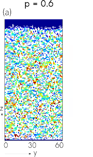
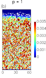
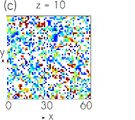
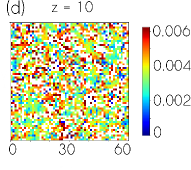
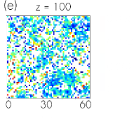
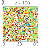
Figure 8: Configurations of the absolute value of the local current in (a),(b) vertical cross sections and (c)-(f) horizontal cross sections. The growth parameter $p$ and the heights of the horizontal sections are indicated. In (a) and (b), the vertical scale is reduced by a factor $2$ for better visualization.

Figs. 9(a) and 9(b) show the distributions $P\left(j\right)$ and $Q\left(j_{z}\right)$, respectively, in films grown with $p=0.6$ and two height intervals: $10\leq z\leq 20$ (lowest points) and $100\leq z\leq 110$ (highest points). The averages and the coefficients of variation of those distributions are presented in Table 1. As $z$ increases, the peaks of the distributions increase, the average currents decrease, and the relative widths decrease. The decrease of $\langle j_{z}\rangle$ is directly related with the increase in the effective porosity because the total current is the same in all horizontal sections. The decrease in $c_{jz}$ means that a more homogeneous current distribution is attained at the highest points. The insets of Figs. 9(a)-(b) show magnified zooms of the distribution tails in log-linear scale; they have faster decay at the highest points, in agreement with the visual observation of a smaller number of large current spots in Figs. 8(c) and 8(e).

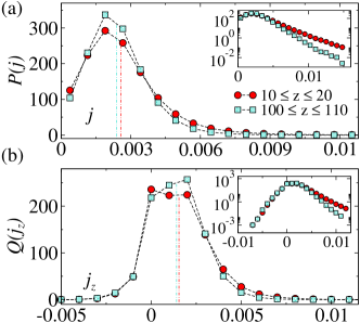
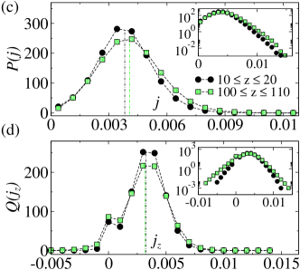
Figure 9: Probability density functions $P\left(j\right)$ of the absolute value of the local current and $Q\left(j_{z}\right)$ of the $z$ component of the local current, for films grown with (a),(b) $p=0.6$ and (c),(d) $p=1$ in two height intervals. Dashed lines connecting the points are drawn to guide the eye. The average values $\langle j\rangle$ and $\langle j_{z}\rangle$ are indicated by vertical dash-dotted lines with the same colors of the corresponding data points. The insets show the distribution tails in loglinear scale.

Figs. 9(c) and 9(d) show the same distributions for $p=1$ and the corresponding averages and coefficients of variation are shown in Table 1. At the highest point, the distributions are wider and their peaks are smaller if compared to the distributions at the lowest point; the magnified zooms in the insets of Figs. 9(c)-(d) confirm that the tails have slower decays at the highest points. The inset of Fig. 9(d) also shows that the fraction of sites with negative $j_{z}$ is larger at the highest points; in those sites, the solute is forced to move in a direction opposite to the average flux to contour the obstacles. Since these films are predominantly grown with BD, this result is interpreted as an effect of the frequent lateral aggregation that blocks vertical paths for the flux.

	$p=0.6$		$p=1$
	$10\leq z\leq 20$	$100\leq z\leq 110$	$10\leq z\leq 20$	$100\leq z\leq 110$
$\langle j\rangle$	$0.00258$	$0.00238$	$0.00381$	$0.00408$
$c_{j}$	$0.639$	$0.538$	$0.379$	$0.399$
$\langle j_{z}\rangle$	$0.00155$	$0.00141$	$0.00324$	$0.00315$
$c_{jz}$	$1.080$	$1.022$	$0.499$	$0.603$

Table 1: Average local currents $\langle j\rangle$ and $\langle j_{z}\rangle$ and coefficients of variation $c_{j}$ and $c_{jz}$ of the distributions in two height intervals, for films grown with $p=0.6$ and $p=1$.

4 Discussion

Here we discuss the relation between macroscopic structural and transport properties (Sec. 4.1), the microscopic interpretation of the nontrivial behavior of the effective diffusion coefficient (Sec. 4.2), the empirical relation between diffusivity and porosity (Sec. 4.3), and possible relations with experimental realizations (Sec. 4.4).

4.1 Growth, structure, and diffusion

In applications of porous media, it is expected that an increase in the porosity favors the diffusivity. This is usually acomplished with changes in the growth conditions. Our model confirms that it is possible with deposition techniques if the relative rate of lateral particle aggregation is increased (i.e. increase of $p$). However, we also showed that larger porosity and larger diffusivity may be obtained without changing the growth conditions, but increasing the film thickness, for films typically with porosity below $0.6$. The opposite trend is observed in the films grown with the largest rates of lateral aggregation, which typically have porosity between $0.6$ and $0.7$ (considering small or large thicknesses).

The tortuosity $\tau$ is useful to quantify and interpret these types of structure-transport relashionships. Here we consider the empirical definition ⁴⁶

$$D_{r}=\frac{\epsilon_{E}}{\tau}.$$ (8)

In the thick film limit, it is generalized as $D_{\infty}=\epsilon_{\infty}/\tau$. In Eq. (8), $\epsilon_{E}$ is interpreted as the main factor to reduce the diffusive current because it reduces the cross sectional area for solute flux; for instance, if the medium has straight channels connecting the two frontiers, we obtain $D_{E}={\epsilon_{E}}D_{0}$ and $\tau=1$. However, if the channels have disordered shapes, the tortuosity represents the additional effects of tortuous paths that the solute is forced to follow to cross the porous medium.

Fig. 10 shows the tortuosities of thin films with $H=50$ and of the thick film limit as function of $p$. It confirms that the structure of the porous films have significant changes when (i) the growth conditions vary (i.e. $p$ varies) and the thickness is constant and (ii) the growth conditions are maintained and the thickness varies. The inset of Fig. 10 highlights the region with large $p$.

Figure 10: Tortuosities calculated in thin films with $H=50$ and in very thick films as a function of $p$. The inset highlight the data for $p\geq 0.7$.

If films with a constant thickness are compared, the tortuosity increases when $p$ decreases, i.e. when the relative rate of film compaction increases. Films with smaller thicknesses are more sentitive to changes in the growth conditions: in thin films with $H=50$, the tortuosity varies from $1.3$ to $440$ as the porosity decreases from $0.66$ to $0.1$; in the thick film limit, a smaller variation is observed, from $1.7$ to $85$, with a change in the porosity from $0.70$ to $0.19$.

When the growth conditions are maintained and the thickness varies, the tortuosity shows the transition between the two kinetic regimes at $p\approx 0.8$, in which the effective porosity is in the range $0.58-0.62$.

In films grown with $p\geq 0.9$, whose porosity range is $0.62-0.70$, $\tau$ is always between $1$ and $2$, and it increases with the thickness. The maximal change in $\tau$ is near $25\%$, which indicates small changes in the pore structure. This is confirmed by the small porosity ratio $r_{\epsilon}$ [Fig. 6(b)]. These films also have small values of the roughness ratio $r_{W}$ (Fig. 5), which shows that the outer surface (where porosity begins to form) evolves slowly as the film grows. We understand that the inherent randomness of the deposition process increases the disorder of the pore system as the film grows, which favors the increase in the tortuosity, and this trend is not compensated by the slow increase in the porosity.

The decrease of $\tau$ with the thickness is observed in films grown with $p\leq 0.7$, whose porosities are below $0.58$. From $H=50$ to the thick film limit, our simulations showed variations in $\tau$ by factors ranging from $\approx 1.3$ ($\epsilon_{\infty}=0.57$) to $\approx 4.7$ ($\epsilon_{\infty}=0.19$). Thus, there are significant changes in the pore systems as these films grow. Indeed, Figs. 5 and 6(b) show larger values of the roughness ratio $r_{W}$ and of the porosity ratio $r_{\epsilon}$ in these conditions. Our interpretation is that the faster widening of the pore system compensates the increasing disorder imposed by the random nature of the deposition process.

4.2 Microscopic interpretation

In films grown with $p=0.6$, Figs. 9(a)-(b) show that the local current distributions are narrower at the highest points. This differs from the high porosity films grown with $p=1$, in which those distributions are wider at the highest points [Figs. 9(c)-(d)].

When particles randomly move in a porous medium, the increase in the tortuosity is related to the presence of obstacles to their random motion. The delays caused by the disorder may be expressed in terms of distributions of waiting times (or hopping times). An increase in the structural disorder is usually associated with an increase in the dispersion of waiting times. For instance, in the case of fractal networks, the self-similar pore size distributions lead to subdiffusion ⁴⁷, i.e. time-decreasing diffusion coefficients; the corresponding distributions of waiting times are also self-similar, which inspires the approaches of continuous time random walks ^{48, 49}. In the present model, the dispersion of waiting times is translated into a dispersion of local currents.

This reasoning leads to a microscopic interpretation of the two kinetic regimes observed here. The distributions in Figs. 9(a)-(b) show that the dispersion of waiting times is smaller at higher points. Thus, the evolution of the local structure with the height is favorable for the increase of the diffusivity. These results, which were shown for films grown with $p=0.6$, are representative of the other films grown with $p\leq 0.7$. However, in the films with $p=1$, Figs. 9(c)-(d) show that the dispersion in the waiting times increases with the height, so the local structure evolution is unfavorable for the diffusion. These results are representative of the films with high porosity, i.e. grown with $p\geq 0.9$. In summary, the decrease in the fluctuations of the local currents combined with the increase in the local porosity are the microscopic features that correlate with the thickness increasing diffusivity.

The macroscopic and the microscopic interpretations presented here are consistent and are based on the calculated global and local quantities, respectively. However, the location of the transition probability $p^{*}$ between the two kinetic regimes cannot be predicted exactly (or with high accuracy) from the available data.

4.3 Relation between diffusion coefficient and porosity

Works on diffusion in porous media frequently obtain empirical power law relations as $D_{r}={\epsilon_{E}}^{m}$, with positive exponents $m$ ⁸, ⁹, ⁸. This type of relation is known as the Archie law ⁵¹. Here we check whether this law is applicable to the films grown with the BD-RDSR model, considering the quantities obtained in the thick film limit.

Fig. 11 shows a bilogarithmic plot of $D_{\infty}$ versus $\epsilon_{\infty}$. It has a downward curvature and, consequently, does not allow a reliable fit of the data in the whole range of porosity studied here. In other words, the empirical Archie law is not applicable to the complete set of porous media generated by the BD-RDSR model.

Figure 11: Diffusion coefficient as a function of the porosity in the thick film limit. Linear fits of the data with $0.5\lesssim\epsilon_{\infty}\lesssim 0.7$ and with $\epsilon_{\infty}\lesssim 0.4$, and the corresponding slopes are shown.

We also tried to fit different parts of the plot in Fig. 11. For the largest porosities, $0.5\lesssim\epsilon_{\infty}\lesssim 0.7$, the fit has a slope $2.05\pm 0.02$, which is close to the values obtained in many natural materials ⁸. However, this fit cannot be extrapolated because it deviates $\approx 10\%$ from the free medium value, $D_{\infty}=1$ for $\epsilon_{\infty}=1$; thus, even in this restricted range of porosity, the Archie relation cannot be consistently used. For the smallest porosities, $\epsilon_{\infty}<0.4$, the porous media are closer to the critical percolation point and the fit has slope $5.2\pm 0.3$. A scaling approach for the diffusion in off-critical conditions ⁴⁷, ³ predicts a slope $4.8\pm 0.2$, which is close to our estimate; see details in Sec. SI.VI of the Supporting Information. However, this should not be interpreted as an application of the Archie law because the fit is also inconsistent with the free medium diffusivity.

4.4 Possible relations with experimental works

The following discussion has a focus on battery electrodes because it was already shown that ion diffusion in their pores frequently is the process that limits the battery performance ⁵³, ⁵⁴. Moreover, experiments and modeling show that adjusting the porosity and the tortuosity by varying the thickness may be a key step to improve electrode efficiency ⁵⁵, ⁵⁶.

In a recent work ⁵⁷, a 13.5 $\mu$m thick pristine carbon porous matrix used in Li-O₂ batteries was shown to have porosity $0.19$ and tortuosity $29.97$, while a discharged cathode had the respective values $0.33$ and $4.80$. Considering the carbon atomic size, the comparison with our model must consider the thick film limit, in which we obtained $\tau=4.50$ for $\epsilon_{\infty}=0.38$ and $\tau=85$ for $\epsilon_{\infty}=0.19$; the first pair of model values is close to the experimental one for the discharged cathode. Another recent work ⁵⁸ presented a carbon binder domain (CBD) of a LiCoO₂ battery with thickness of a few micrometers, porosity $0.58$, and tortuosity $2.3-3.5$. For this porosity, our model gives $\tau\approx 2.1$, which is also close to the experimental estimates. Finally, a study of calendered, negative electrodes ($\sim 100\mu$m thick) without CBD show porosities $0.35-0.40$ and tortuosities $4.9-5.9$ ⁵⁹. Interpolation of the model data in Fig. 10 gives $\tau=4.2--6.5$ in the same porosity range. Thus, despite the strong approximations of the BD-RDSR model, it leads to relations between porosity and tortuosity that are quantitatively close to experimental values.

We are not aware of processes in which the growth conditions were maintained and an increase in the diffusivity was observed. However, in growth of composition graded films, the physical conditions were dynamically changed to increase the porosity and to decrease the tortuosity with the thickness ⁶⁰, ⁶¹. Despite that difference, our results may be helpful to applications using this technique; for instance, if the porosity formation is controlled by the adsorption, a rapid increase of the roughness with the thickness may anticipate a favorable evolution of the pore system.

On the other hand, in a recent study with reduced graphene oxide (ErGO) electrodes produced by electrodeposition, the electrolyte diffusivity was shown to decrease nearly $4$ times as the film thickness increases from $3\mu$m to $79\mu$m ⁶². In this case, it is possible that the deposition kinetics is (at least partially) responsible for the decrease in the diffusivity, as in the regime of thickness-hampered transport of our model. If the electrodeposition conditions can be controlled in this system, we believe that it is a potential candidate for an experimental search of the transition to a regime of thickness-facilitated transport, as suggested by the model.

In any application, the benefits or disadvantages of the results presented here have to be correlated with other effects of increasing a film thickness. For energy storage applications, larger thicknesses are usually favorable to increase the areal energy density. Thus, if the regime of thickness-facilitated transport (medium to low porosities in our model) is applicable, the beneficial effect to ion diffusion is an additional reason to deposit thicker films. However, in the regime of thickness-hampered transport, the increase in the tortuosity with the thickness is relatively small ($\lesssim 25\%$), so this should not be a major concern in comparison with the energetic advantage of thicker films. Thus, whenever the deposition conditions are consistent with the approximations of the present model, we generally expect that the increase of thickness is helpful for energy storage applications, even if there is a small loss in diffusivity.

At this point, it is important to highlight the physical conditions considered in the model studied here: the particle flux towards the deposit must be (at least partially) collimated, the relaxation of deposited particles is of short range, and subsurface relaxation during the growth is negligible. Alternatively, the relaxation mechanism could consider preferential aggregation at the sites with the largest numbers of NN bonds instead of the sites with the lowest heights, for instance using the models of Das Sarma and Tamborenea ⁶³ and of Wolf and Villain ⁶⁴. However, there is numerical evidence that these two models are in the same growth class (EW) of RDSR in 3D ⁶⁵. Thus, mixing the BD rules and the rules of one of those models will also lead to a competitive KPZ-type model, in which the porosity is expected to increase with the thickness for a fixed $p$. The thickness dependence of the diffusion coefficient cannot be predicted from these properties, but the above similarities suggest that the dependence may be the same as that of BD-RDSR. On the other hand, if the mobility of the adsorbed particles is large and they can eventually fill distant pores, then more drastic changes in the film structure are expected and the conclusions drawn from BD-RDSR may fail.

5 Conclusion

We studied the relation between the growth kinetics of porous films, their surface and bulk structures, and the diffusive transport of a solute in their pores. We used a deposition model in a lattice in which a single parameter controls the relative rates of lateral aggregation of incident particles (responsible for pore formation) and of relaxation after deposition (responsible for compaction of the deposits). When the deposition conditions change by increasing this rate, we always observe the increase of the growth velocity, of the surface roughness, of the effective porosity, and of the diffusivity.

We also compared films produced in the same growth conditions but with different thickness. As the thickness increases, the effective porosity slowly increases; this is the same trend predicted for the total porosity by the KPZ theory of interface roughening. In films with porosity below $0.58$, the effective diffusion coefficient increases with the thickness. This is partly due to the increase of porosity, but mostly due the decrease of the tortuosity. For instance, comparing films whose thicknesses correspond to $50$ and to $\geq{10}^{4}$ layers of particles, the tortuosity may be reduced by a factor $\sim 5$ while the porosity increases by a factor $\sim 2$. At microscopic level, we observed that the distributions of local solute currents in these deposits are narrower at higher points, i.e. the currents are more uniform. This indicates smaller dispersion in the waiting times of the diffusing species and qualitatively explains the thickness-facilitated transport. In films with porosities $\sim 0.65-0.7$ (the maximal values obtained with the model), the tortuosity decreases with the thickness, but the maximal changes are near $25\%$. This regime of thickness-hampered transport is characterized by larger widths of the local current distributions at higher points.

The values of porosity and tortuosity in thick films are close to the values obtained in porous electrodes produced with different techniques ⁵⁷, ⁵⁸, ⁵⁹. Thus, despite the simple stochastic rules of our model, it may be reasonable to predict qualitative relations between growth, structure and diffusive transport in porous materials of technological interest. Quantitative relations are expected to be predicted by simulations of improved models which account for details of particular growth processes. Possible extensions may consider the effects of non-collimated particle flux and longer diffusion lenghts of the adsorbed species, as shown in recent models that reproduce morphological properties of dendritic films ⁶⁶, ⁶⁷, ⁶⁸. In these cases, the dendrite orientations and the porosity variations that are expected due to the growth instabilities should affect the pore diffusivity.

We also believe that the results presented here or extensions of our approach may be useful to study porous media other than electrodes, and of interest in different areas. For instance, diffusion simulations were recently performed in models of deposited porous media proposed for sedimentary rocks ⁶⁹, but no thickness effect was analyzed. From a point of view of fundamental science, the transition predicted between kinetic regimes of thickness-facilitated and thickness-hampered transport may be of interest both for experimental investigation and for mathematical treatment.

The Supporting Information file shows details of the simulations, the method to calculate the effective diffusion coefficients, the evolution of the growth velocity, the extrapolation of the porosity to the thick film limit, the variations of the numbers of connected domains, and the scaling approach for diffusion coefficient in low porosities.

SI.I Simulations of film growth and calculation of structural properties

The calculation of average thickness, roughness, and total porosity depends only on the configuration of the top outer surface. For several values of $p$, those quantities were averaged in $300$ film configurations with lateral size $L=512a$ and grown up to $t_{g}\approx{10}^{3}$, which provides results with accuracy $\lesssim 1\%$.

The enumeration of connected porous domains and the calculation of the effective porosity requires knowledge from the whole film configuration between the two frontiers. Counting of connected domains was performed by a three-dimensional Hoshen-Kopelman code ¹. Average quantities were obtained out of 300 samples for lateral size $L=512a$ and out of 1000 samples for lateral sizes $L=128a$ and $256a$. Apart from $p=0.4$, neither appreciable finite-size nor finite-sampling effects were observed.

SI.II Simulations of diffusive transport

Simulation of infiltration begins with no solute in the pores. We measure the solute currents $J_{in}$ at the substrate ($z=0$) and $J_{out}$ near the outer surface ($z/a=H$). These currents are defined as the numbers of molecules flowing into and out of the pore system, respectively, per unit flat area $L^{2}$ and unit time. After some time, the system reaches a steady state, in which these two currents fluctuate around the same value. This is illustrated in Fig. S1.

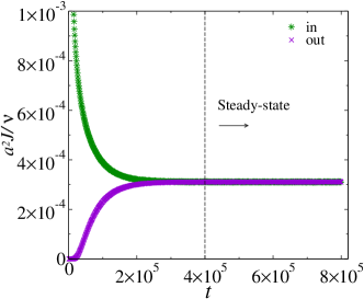
Figure S1: Time evolution of the scaled currents flowing into and out of the films grown with $p=1$ up to $t_{g}=70$ (thickness $H\approx 225$ and total porosity $\epsilon_{T}\approx 0.69$).

In a medium with thickness $H$, the average distance between the source and the drain is $H+1$. In steady state transport, the average value of the current, $J_{s}$, is related to the effective diffusion coefficient of the solute, $D_{E}$, by $J_{s}=D_{E}/\left[\left(H+1\right)a^{4}\right]$ (first Fick law). In a three dimensional free medium, the diffusion coefficient is $D_{0}=\nu a^{2}/6$. The effective diffusion coefficient is consequently given by Eq. (6) of the main text, The dimensionless current $J_{s}a^{2}/\nu$ is directly determined in the simulations, as illustrated in Fig. S1. In any disordered system, we expect that $D_{E}/D_{0}<1$.

An alternative method to probe the effect of a disordered medium on diffusion processes is the release of non-interacting random walkers, or tracers, in that medium. To avoid effects of the finite system size (including the thickness), the tracers are released far from the borders and the choice of the maximal walking time has to warrant a negligible probability of reaching those borders. However, our aim is to model systems with mass flux across the sample and to determine thickness effects. In this case, the approach described above is more appropriate than tracer diffusion simulations.

The simulation of transport is the most time consuming part of our numerical work. For each configuration of the film (grown with a given $p$), the calculation has to be separately performed in several thicknesses and, for each thickness, convergence to the steady state is necessary. Reaching the steady state takes a time of order $H^{2}/\nu$ in the samples with higher porosity ($\sim 70\%$), but may be two orders of magnitude slower in tortuous media with low porosity ($\lesssim 20\%$). In the timescale $1/\nu$, it is necessary to update the positions of a number of solute molecules of order $\epsilon_{E}{\left(L/a\right)}^{2}H$, so the total number of updates in a given simulation is, at least, of order $\epsilon_{E}{\left(L/a\right)}^{2}H^{3}$.

For these reasons, most simulations of diffusive transport were performed in lateral sizes $L/a=64$ and $128$ and thicknesses $H\approx 300$ or smaller. For each $p\geq 0.45$ and $20$-$30$ values of the thickness $H$, $40$ film configurations were generated for these calculations. The comparison of results in sizes $L/a=64$ and $128$ showed weak effects of the finite size $L$. Some films with smaller thicknesses were also simulated in size $L=256$ to confirm this trend. For $p=0.4$, finite-size effects in $L/a=128$ were observed because these films are closer to the critical percolation point; consequently, we performed simulations in $L/a=256$.

SI.III Evolution of the thickness

Fig. S2(a) shows the time evolution of the thickness for $p\geq 0.4$. The good linearity observed at long times indicate that the growth velocities converge to constant values in large thicknesses. Fig. S2(b) shows the dimensionless growth velocity $v_{g}$ [Eq. (7) of the main text] as a function of $1/t_{g}$, which facilitates the observation of the time increase of $v_{g}$.

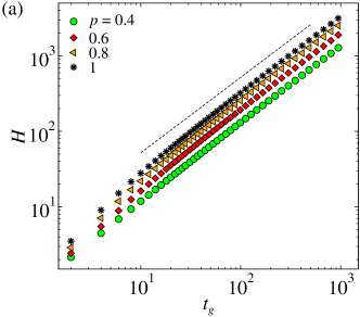
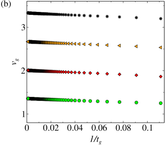
Figure S2: (a) Average film thickness as function of the growth time for several values of $p$. The uncertainties are smaller than the size of the symbols. (b) Growth velocity estimated in time intervals $\Delta t_{g}=2$ as a function of the reciprocal of the growth time for several values of $p$.

SI.IV Extrapolation of the porosity to the thick film limit

Based on Eq.(9) of the paper, we propose similar scaling relation for the effective porosity:

$$\epsilon_{E}\approx\epsilon_{\infty}-\frac{B}{t_{g}^{\lambda}},$$ (S1)

where $\epsilon_{\infty}$, $B$, and $\lambda$ are positive constants. Figs. S3(a) and S3(b) show $\epsilon_{E}$ as a function of $1/t_{g}^{\lambda}$ for $p=0.7$ and $p=1$, respectively, using the values of $\lambda$ that provide the best linear fits in each case.

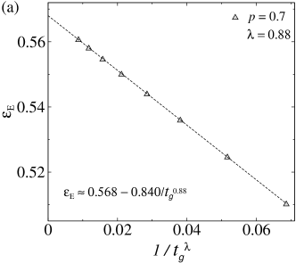
Figure S3: Effective porosity as function of $1/t_{g}^{\lambda}$ for (a) $p=0.7$ and (b) $p=1$, with the values of $\lambda$ indicated in each plot. Dashed lines are linear fits of the data.

The fits to Eq. (S1) provide estimates of $\epsilon_{\infty}$, which are the effective porosities in the thick film limit. In all cases, this is expected to be the effective porosity of films with $H\geq{10}^{4}$ with accuracy $\lesssim 1\%$.

SI.V Number of connected domains

Fig. S4 shows the average number of connected porous domains $\Pi$ for several values of $p$. For $0.5\leq p\leq 1$, a single domain is observed in films with $H\gtrsim 20$; for $p=0.4$, this is observed with $H\gtrsim 60$.

Figure S4: Average number of connected porous domains as function of the average thickness. Results are obtained in size $L=512a$ and averaging over 300 samples. The inset shows a zoom of the region near $\Pi=1$.

SI.VI Diffusion coefficient in low porosities

A check of the reliability of our calculations of diffusion coefficients is their behavior for low effective porosity, in which the pore systems are close to the critical percolation point located at $p_{c}\approx 0.35$ ². Let $\epsilon_{c}$ be the value of the total porosity at this critical point. In the connected porous domain, a scaling approach ^{3, 4} predicts that the diffusion coefficient of a random walker scales as $D_{T}\sim{\left(\epsilon_{T}-\epsilon_{c}\right)}^{\tilde{\mu}\nu_{p}-\beta_{p}}$, where $\tilde{\mu}$ is termed conductivity exponent and $\nu_{p}$ and $\beta_{p}$ stand for percolation exponents. Here, the total pore volume fraction $\epsilon_{T}$ parallels the occupation probability of lattice models with random distributions of occupied and empty sites ^{5, 4}.

The diffusion coefficient $D_{T}$ is reduced in comparison with the free medium value only due to the tortuous paths of the porous medium, while the effective diffusion coefficient also decreases due to the restricted pore volume in which the solute moves; thus, they are related as $D_{E}=\phi_{E}D_{T}$. In the notation of the thick film limit used here, if $D_{T}$ is normalized by the free medium diffusivity, we have $D_{\infty}=\epsilon_{\infty}D_{T}$.

Basic percolation theory also sets that the effective porosity close to the critical point scales as $\epsilon_{\infty}\sim{\left(\epsilon_{T}-\epsilon_{c}\right)}^{\beta_{p}}$ ⁵; this is the relation that originally defines the exponent $\beta_{p}$. Considering the scaling relations between percolation exponents ^{5, 4}, we obtain

$$D_{E}\sim{\epsilon_{\infty}}^{q}\qquad,\qquad q=\frac{\tilde{\mu}}{3-d_{f}},$$ (S2)

where $d_{f}$ is the fractal dimension of the critical percolation cluster. The available numerical estimates $\tilde{\mu}=2.26\left(4\right)$ ⁶ and $d_{f}=2.53\left(4\right)$ ⁷ give $q=4.8\left(2\right)$, which is close to the numerical estimate $5.2\pm 0.3$ shown in the main text. Here, $q$ plays a role similar to the cementation exponent $m$ of the Archie law ⁸, but Eq. (S2) does not fit the values of $D_{E}$ in large porosities.

References

- Li et al. 2017 Li, J.; Du, Z.; Ruther, R. E.; An, S. J.; David, L. A.; Hays, K.; Wood, M.; Phillip, N. D.; Sheng, Y.; Mao, C. et al. Toward low-cost, high-energy density, and high-power density lithium-ion batteries. J. Occup. Med. 2017, 69, 1484–1496
- Wang et al. 2020 Wang, F.; Li, X.; Hao, X.; Tan, J. Review and recent advances in mass transfer in positive electrodes of Aprotic Li-O2 Batteries. ACS Appl. Energy Mater. 2020, 3, 2258–2270
- Koros and Zhang 2017 Koros, W. J.; Zhang, C. Materials for next-generation molecularly selective synthetic membranes. Nat. Mater. 2017, 16, 289–297
- Lin et al. 2019 Lin, R.-B.; Xiang, S.; Li, B.; Cui, Y.; Qian, G.; Zhou, W.; Chen, B. Our journey of developing multifunctional metal-organic frameworks. Coord. Chem. Rev. 2019, 384, 21–36
- Santamaría-Holek et al. 2019 Santamaría-Holek, I.; Hernández, S. I.; García-Alcántara, C.; Ledesma-Durán, A. Review on the macro-transport processes theory for irregular pores able to perform catalytic reactions. Catalysis 2019, 9, 281
- Zheng et al. 2018 Zheng, Y.; Geng, H.; Zhang, Y.; Chen, L.; Li, C. C. Precursor-based synthesis of porous colloidal particles towards highly efficient catalysts. Chem. Eur. J. 2018, 24, 10280–10290
- Heubner et al. 2020 Heubner, C.; Langklotz, U.; Lämmel, C.; Schneider, M.; Michaelis, A. Electrochemical single-particle measurements of electrode materials for Li-ion batteries: Possibilities, insights and implications for future development. Electrochim. Acta 2020, 330, 135160
- Dullien 1979 Dullien, F. A. L. Porous Media, Fluid Transport and Pore structure; Academic: San Diego, 1979
- Adler 1992 Adler, P. M. Porous Media: Geometry and Transports; Butterworth-Heinemann: Stoneham, MA, USA, 1992
- Guyont et al. 1987 Guyont, E.; Oger, L.; Plona, T. J. Transport properties in sintered porous media composed of two particle sizes. J. Phys. D: Appl. Phys. 1987, 20, 1637–1644
- Kim and Torquato 1991 Kim, I. C.; Torquato, S. Effective conductivity of suspensions of hard spheres by Brownian motion simulation. J. Appl. Phys. 1991, 69, 2280–2289
- Coelho et al. 1997 Coelho, D.; Thovert, J.-F.; Adler, P. M. Geometrical and transport properties of random packings of spheres and aspherical particles. Phys. Rev. E 1997, 55, 1959–1978
- Tomadakis and Sotirchos 1993 Tomadakis, M. M.; Sotirchos, S. Ordinary and transition regime diffusion in random fiber structures. AIChE J. 1993, 39, 397–412
- Sund et al. 2017 Sund, N. L.; Porta, G. M.; Bolster, D. Upscaling of dilution and mixing using a trajectory based Spatial Markov random walk model in a periodic flow domain. Adv. Water Res. 2017, 103, 76–85
- Müter et al. 2015 Müter, D.; Sorensen, H. O.; Bock, H.; Stipp, S. L. S. Particle Diffusion in Complex Nanoscale Pore Networks. J. Phys. Chem. C 2015, 119, 10329–10335
- Tallarek et al. 2019 Tallarek, U.; Hlushkou, D.; Rybka, J.; Höltzel, A. Multiscale simulation of diffusion in porous media: From interfacial dynamics to hierarchical porosity. J. Phys. Chem. C 2019, 123, 15099–15112
- Jiang et al. 2017 Jiang, Z. Y.; Qu, Z. G.; Zhou, L.; Tao, W. Q. A microscopic investigation of ion and electron transport in lithium-ion battery porous electrodes using the lattice Boltzmann method. Applied Energy 2017, 194, 530–539
- Torayev et al. 2018 Torayev, A.; Magusin, P. C. M. M.; Grey, C. P.; Merlet, C.; Franco, A. A. Importance of incorporating explicit 3D-resolved electrode mesostructures in Li-O2 battery models. ACS Appl. Energy Mater. 2018, 1, 6433–6441
- Elabyouki et al. 2019 Elabyouki, M.; Bahamon, D.; Khaleel, M.; Vega, L. F. Insights into the transport properties of electrolyte solutions in a hierarchical carbon electrode by molecular dynamics simulations. J. Phys. Chem. C 2019, 123, 27273–27285
- Tan et al. 2019 Tan, C.; Kok, M. D. R.; Daemi, S. R.; Brett, D. J. L.; Shearing, P. R. Three-dimensional image based modelling of transport parameters in lithium-sulfur batteries. Phys. Chem. Chem. Phys. 2019, 21, 4145–4154
- Barabási and Stanley 1995 Barabási, A.-L.; Stanley, H. E. Fractal Concepts in Surface Growth; Cambridge University Press: New York, USA, 1995
- Vold 1959 Vold, M. J. Sediment volume and structure in dispersions of anisometric particles. J. Phys. Chem. 1959, 63, 1608–1612
- Family 1986 Family, F. Scaling of rough surfaces: Effects of surface diffusion. J. Phys. A: Math. Gen. 1986, 19, L441
- Liu et al. 2017 Liu, Z.; Wood III, D. L.; Mukherjee, P. P. Evaporation induced nanoparticle - binder interaction in electrode film formation. Phys. Chem. Chem. Phys. 2017, 19, 10051–10061
- Lehnen and Lu 2010 Lehnen, C.; Lu, T. Morphological evolution in ballistic deposition. Phys. Rev. E 2010, 82, 085437
- Hoshen and Kopelman 1976 Hoshen, J.; Kopelman, R. Percolation and cluster distribution. I. Cluster multiple labeling technique and critical concentration algorithm. Phys. Rev. B 1976, 14, 3438–3445
- Stauffer and Aharony 1992 Stauffer, D.; Aharony, A. Introduction to Percolation Theory; Taylor & Francis: London/Philadelphia, 1992
- Aarão Reis 2016 Aarão Reis, F. D. A. Scaling relations in the diffusive infiltration in fractals. Phys. Rev. E 2016, 94, 052124
- Reis and Voller 2019 Reis, F. D. A. A.; Voller, V. R. Models of infiltration into homogeneous and fractal porous media with localized sources. Phys. Rev. E 2019, 99, 042111
- Krug 1997 Krug, J. Origins of scale invariance in growth processes. Adv. Phys. 1997, 46, 139–282
- Kardar et al. 1986 Kardar, M.; Parisi, G.; Zhang, Y.-C. Dynamic scaling of growing interfaces. Phys. Rev. Lett. 1986, 56, 889–892
- Kelling et al. 2016 Kelling, J.; Ódor, G.; Gemming, S. Universality of (2+1)-dimensional restricted solid-on-solid models. Phys. Rev. E 2016, 94, 022107
- Kertész and Wolf 1988 Kertész, J.; Wolf, D. E. Noise reduction in Eden models: II. Surface structure and intrinsic width. J. Phys. A: Math. Gen. 1988, 21, 747–761
- Alves et al. 2014 Alves, S. G.; Oliveira, T. J.; Ferreira, S. C. Origins of scaling corrections in ballistic growth models. Phys. Rev. E 2014, 90, 052405
- Krug 1990 Krug, J. Universal finite-size effects in the rate of growth processes. J. Phys. A: Math. Gen. 1990, 23, L987–L994
- Edwards and Wilkinson 1982 Edwards, S. F.; Wilkinson, D. R. The surface statistics of a granular aggregate. Proc. R. Soc. Lond. A 1982, 381, 17–31
- Pellegrini and Jullien 2000 Pellegrini, Y. P.; Jullien, R. Roughening transition and percolation in random ballistic deposition. Phys. Rev. Lett. 2000, 64, 1745–1748
- Canet et al. 2010 Canet, L.; Chaté, H.; Delamotte, B.; Wschebor, N. Nonperturbative renormalization group for the Kardar-Parisi-Zhang equation. Phys. Rev. Lett. 2010, 104, 150601
- Chame and Reis 2002 Chame, A.; Reis, F. D. A. A. Crossover effects in a discrete deposition model with Kardar-Parisi-Zhang scaling. Phys. Rev. E 2002, 66, 051104
- Muraca et al. 2004 Muraca, D.; Braunstein, L. A.; Buceta, R. C. Universal behavior of the coefficients of the continuous equation in competitive growth models. Phys. Rev. E 2004, 69, 065103
- Silveira and Aarão Reis 2012 Silveira, F. A.; Aarão Reis, F. D. A. Langevin equations for competitive growth models. Phys. Rev. E 2012, 85, 011601
- Kriston et al. 2016 Kriston, A.; Pfrang, A.; Boon-Brett, L. Development of multi-scale structure homogenization approaches based on modeled particle deposition for the simulation of electrochemical energy conversion and storage devices. Electrochim. Acta 2016, 201, 380–394
- Katzav et al. 2006 Katzav, E.; Edwards, S. F.; Schwartz, M. Structure below the growing surface. Europhys. Lett. 2006, 75, 29–35
- Yu and Amar 2002 Yu, J.; Amar, J. G. Scaling behavior of the surface in ballistic deposition. Phys. Rev. E 2002, 65, 060601(R)
- Reis and di Caprio 2014 Reis, F. D. A. A.; di Caprio, D. Crossover from anomalous to normal diffusion in porous media. Phys. Rev. E 2014, 89, 062126
- Cussler 2007 Cussler, E. L. Diffusion: Mass Transfer in Fluid Systems, 3rd ed.; Cambridge University Press: Cambridge, UK, 2007
- Ben-Avraham and Havlin 2000 Ben-Avraham, D.; Havlin, S. Diffusion and Reactions in Fractals and Disordered Systems; Cambridge University Press: Cambridge, UK, 2000
- Bouchaud and Georges 1990 Bouchaud, J. P.; Georges, A. Anomalous diffusion in disordered media: Statistical mechanisms, models and physical applications. Phys. Rep. 1990, 195, 127–293
- Metzler et al. 2014 Metzler, R.; Jeon, J.-H.; Cherstvya, A. G.; Barkai, E. Anomalous diffusion models and their properties: non-stationarity, non-ergodicity, and ageing at the centenary of single particle tracking. Phys. Chem. Chem. Phys. 2014, 16, 24128–24164
- Grathwohl 1998 Grathwohl, P. Diffusion in natural porous media: contaminant transport, sorption/desorption and dissolution kinetics; Springer: New York, USA, 1998
- Archie 1942 Archie, G. : The electrical resistivity log as an aid in determining some reservoir characteristics. Trans. AIME 1942, 146, 54–61
- Havlin et al. 1983 Havlin, S.; ben Avraham, D.; Sompolinsky, H. Scaling behavior of diffusion on percolation clusters. Phys. Rev. A 1983, 27, 1730–1733
- Gao et al. 2018 Gao, H.; Wu, Q.; Hu, Y.; Zheng, J. P.; Amine, K.; Chen, Z. Revealing the rate-limiting Li-ion diffusion pathway in ultrathick electrodes for Li-ion batteries. J. Phys. Chem. Lett. 2018, 9, 5100–5104
- Hossain et al. 2019 Hossain, M. S.; Stephens, L. I.; Hatami, M.; Ghavidel, M.; Chhin, D.; Dawkins, J. I. G.; Savignac, L.; Mauzeroll, J.; Schougaard, S. B. Effective mass transport properties in lithium battery electrodes. ACS Appl. Energy Mater. 2019, 3, 440–446
- Dai and Srinivasan 2016 Dai, Y.; Srinivasan, V. On graded electrode porosity as a design tool for improving the energy density of batteries. J. Electrochem. Soc. 2016, 163, A406–A416
- Colclasure et al. 2020 Colclasure, A. M.; Tanim, T. R.; Jansen, A. N.; Trask, S. E.; Dunlop, A. R.; Polzin, B. J.; Bloom, I.; Robertson, D.; Flores, L.; Evans, M. et al. Electrode scale and electrolyte transport effects on extreme fast charging of lithium-ion cells. Electrochim. Acta 2020, 337, 135854
- Su et al. 2020 Su, Z.; De Andrade, V.; Cretu, S.; Yin, Y.; Wojcik, M. J.; Franco, A. A.; Demortière, A. X-ray nanocomputed tomography in Zernike phase contrast for studying 3D morphology of Li-O2 battery electrode. ACS Appl. Energy Mater. 2020, 3, 4093–4102
- Vierrath et al. 2015 Vierrath, S.; Zielke, L.; Moroni, R.; Mondon, A.; Wheeler, D. R.; Zengerle, R.; Thiele, S. Morphology of nanoporous carbon binder domains in Li-ion batteries - A FIB-SEM study. Electrochem. Comm. 2015, 60, 176–179
- Usseglio-Viretta et al. 2018 Usseglio-Viretta, F. L. E.; Colclasure, A.; Mistry, A. N.; Claver, K. P. Y.; Pouraghajan, F.; Finegan, D. P.; Heenan, T. M. M.; Abraham, D.; Mukherjee, P. P.; Wheeler, D. et al. Resolving the discrepancy in tortuosity factor estimation for Li-ion battery electrodes through micro-macro modeling and experiment. J. Electrochem. Soc. 2018, 165, A3403–A3426
- Liu et al. 2017 Liu, L.; Guan, P.; Liu, C. Experimental and simulation investigations of porosity graded cathodes in mitigating battery degradation of high voltage lithium-ion batteries. J. Electrochem. Soc. 2017, 164, A3163–A3173
- Cheng et al. 2020 Cheng, C.; Drummond, R.; Duncan, S. R.; Grant, P. S. Combining composition graded positive and negative electrodes for higher performance Li-ion batteries. J. Power Sources 2020, 448, 227376
- Zhan et al. 2020 Zhan, Y.; Edison, E.; Manalastas, W.; Tan, M. R. J.; Buffa, R. S. A.; Madhavi, S.; Mandler, D. Electrochemical deposition of highly porous reduced graphene oxide electrodes for Li-ion capacitors. Electrochim. Acta 2020, 337, 135861
- Das Sarma and Tamborenea 1991 Das Sarma, S.; Tamborenea, P. A new universality class for kinetic growth: One-dimensional molecular-beam epitaxy. Phys. Rev. Lett. 1991, 66, 325–328
- Wolf and Villain 1990 Wolf, D. E.; Villain, J. Growth with Surface Diffusion. EPL (Europhysics Letters) 1990, 13, 389
- Chame and Reis 2004 Chame, A.; Reis, F. D. A. A. Scaling of local interface width of statistical growth models. Surface Science 2004, 553, 145 – 154
- Aryanfar et al. 2015 Aryanfar, A.; Cheng, T.; Colussi, A. J.; Merinov, B. V.; Goddard III, W. A.; Hoffmann, M. R. Annealing kinetics of electrodeposited lithium dendrites. J. Chem. Phys. 2015, 143, 134701
- Reis et al. 2017 Reis, F. D. A. A.; di Caprio, D.; Taleb, A. Crossover from compact to branched films in electrodeposition with surface diffusion. Phys. Rev. E 2017, 96, 022805
- Vishnugopi et al. 2020 Vishnugopi, B. S.; Hao, F.; Verma, A.; Mukherjee, P. P. Surface diffusion manifestation in electrodeposition of metal anodes. Phys. Chem. Chem. Phys. 2020, 22, 11286–11295
- Giri et al. 2013 Giri, A.; Tarafdar, S.; Gouze, P.; Dutta, T. Fractal geometry of sedimentary rocks: simulation in 3-D using a Relaxed Bidisperse Ballistic Deposition Model. Geophys. J. Int. 2013, 192, 1059–1069
Supporting Information
Effects of the Growth Kinetics on Solute Diffusion in Porous Films
Gabriela B. Correa1,∗, Renan A. L. Almeida1,†, and Fábio D. A. Aarão Reis1,‡
1Instituto de Física, Universidade Federal Fluminense, Avenida Litorânea s/n, 24210-340 Niterói, RJ, Brazil
E-mail: ∗gabriela_barreto@id.uff.br; †renan.lisboa@ufv.br; ‡reis@if.uff.br

References

- 1 J. Hoshen and R. Kopelman. Percolation and cluster distribution. I. Cluster multiple labeling technique and critical concentration algorithm. Phys. Rev. B, 14:3438–3445, 1976.
- 2 Jianguo Yu and Jacques G. Amar. Scaling behavior of the surface in ballistic deposition. Phys. Rev. E, 65:060601(R), 2002.
- 3 S. Havlin, D. ben Avraham, and H. Sompolinsky. Scaling behavior of diffusion on percolation clusters. Phys. Rev. A, 27:1730–1733, 1983.
- 4 S. Havlin and D. Ben-Avraham. Diffusion in disordered media*. Adv. Phys., 51:187–292, 2002.
- 5 D. Stauffer and A. Aharony. Introduction to Percolation Theory. Taylor & Francis, London/Philadelphia, 1992.
- 6 J. M. Normand and H. J. Herrmann. Precise determination of the conductivity exponent of 3D percolation using "Percola". Int. J. Mod. Phys. C, 6:813–817, 1995.
- 7 N. Jan and D. Stauffer. Random site percolation in three dimensions. Int. J. Mod. Phys. C, 9:341–347, 1998.
- 8 P. Grathwohl. Diffusion in natural porous media: contaminant transport, sorption/desorption and dissolution kinetics. Springer, New York, USA, 1998.