/prAtEnd/global custom defaults/.style= text link= LABEL:proof:prAtEnd\pratendcountercurrent, text proof=of \autorefthm:prAtEnd\pratendcountercurrent
A Decentralized Primal-Dual Framework for Non-convex Smooth Consensus Optimization
Abstract
In this work, we introduce ADAPD, A DecentrAlized Primal-Dual algorithmic framework for solving non-convex and smooth consensus optimization problems over a network of distributed agents. The proposed framework relies on a novel problem formulation that elicits ADMM-type updates, where each agent first inexactly solves a local strongly convex subproblem with any method of its choice and then performs a neighbor communication to update a set of dual variables. We present two variants that allow for a single gradient step for the primal updates or multiple communications for the dual updates, to exploit the tradeoff between the per-iteration cost and the number of iterations. When multiple communications are performed, ADAPD can achieve theoretically optimal communication complexity results for non-convex and smooth consensus problems. Numerical experiments on several applications, including a deep-learning one, demonstrate the superiority of ADAPD over several popularly used decentralized methods.
Index Terms:
non-convex consensus optimization, decentralized optimization, primal-dual method, decentralized learning.I Introduction
Given a set of agents connected by an undirected network (graph) , where denotes the set of agents and denotes the set of feasible local communications among agents, consensus optimization methods solve the following problem using only local computation and local communication,
| (1) |
where each is a differentiable, potentially non-convex, cost function known only to agent .
Problem (1) arises naturally in various scientific and engineering applications such as distributed machine learning/federated learning [1, 2, 3], decentralized matrix factorization [4], network sensing and localization [5, 6, 7], and multi-vehicle coordination [8], to name a few. The decision variable can represent the weights of a neural network [1], the location of a particular object [8], or the state of a smart grid system [6], for example. Essentially, any scenario in which data is either too large or naturally distributed fits problem (1).
I-A Problem Formulation
It is well known [6, 9] that if is connected, the following problem is equivalent to (1):
| (2) |
where is a mixing matrix [6, 10, 11] that satisfies the conditions in Assumption 1 below, and
| (3) |
is the concatenation of local decision variables and the global objective function, respectively, written in matrix notation. Here, is agent ’s local copy of the global variable , and represents the connectivity structure of the network .
Assumption 1
The mixing matrix, , satisfies,
-
(i)
(Decentralized property) if , otherwise ,
-
(ii)
(Symmetric property)
-
(iii)
(Null space property) , where is the vector of all ones, and
-
(iv)
(Spectral property) the eigenvalues of lie in the range and can be ordered as
Several common choices for mixing matrices are presented in [6].
-
-
Laplacian-based constant edge weight matrix,
(4) where L is the Laplacian matrix of and Here, is the largest positive eigenvalue of If the eigenvalues of L are unknown, by the Gershgorin circle theorem one can use , for some , where is the set of agents that can communicate with agent .
-
-
Metropolis constant edge weight matrix, for some ,
(5) -
-
Symmetric fastest distributed linear averaging matrix, (FDLA), which is a matrix that achieves the fastest information diffusion through and is obtained by solving a semidefinite program [12].
Note that the constraint formulation in (2) is not the only choice for a consensus problem. Under Assumption 1, an equivalent consensus constraint adopted by others [13, 4, 14] is for all This constraint is an edge-based constraint, whereas we consider a vertex-based constraint. When a primal-dual approach is designed, if is dense, then a vertex-based constraint introduces fewer dual variables than an edge-based constraint. Further, an optimal can be designed, given [12].
A vital quantity for our analysis comes from the spectral properties of . We define
| (6) |
The metric in (6) is one way to measure the connectivity of , where implies good connectivity.
Under Assumption 1, particularly , a further equivalent reformulation to (1) is
| (7) |
where is the matrix of all zeros. A benefit of this formulation is that the constraint can now be incorporated into a penalty term, , where is a penalty parameter. The gradient associated with this term is , which can be computed by a single neighbor communication.
One way to solve (7) is to form the augmented Lagrangian with dual variables and perform a primal-dual type update as in IDEAL [15]. The issue with this approach is that the communication and computation phases are inherently coupled, illustrated as follows. The classic primal-dual updates at iteration used to solve (7) are
| (8) |
If a first-order method is used to solve the subproblem, then part of the gradient will contain at each gradient computation, thus for every gradient computed, one neighbor communication must be performed.
Another way to solve (7), as suggested by the Prox-PDA method [4], is to introduce an additional proximal term of the form , where with some diagonal matrix . This negates the neighbor communication required in the subproblem of (8), but introduces a new parameter that impacts this method’s numerical performance.
Interestingly, Prox-PDA with a special choice of recovers the distributed ADMM algorithm [16] for consensus optimization with edge-based constraint; see Appendix B for details. Hence, part of this work serves to compare ADMM-type methods derived from using edge-based constraints versus vertex-based constraints for solving problem (1) in a decentralized manner. Our numerical findings in Section IV indicate that our below derived inexact ADMM gives better performance than distributed ADMM [16].
To remove the addition of from Prox-PDA, yet still decouple the communication and computation phases of traditional primal-dual methods, we propose adding an extra variable (and constraint), leading to the following formulation:
| (9) |
Governed now by two blocks of primal variables, a natural approach to solve (9) would be to use an ADMM-type update [17, 18], but as argued in Section II, the classic ADMM cannot be implemented in a decentralized manner to solve (9). Hence, we are motivated to design a method that: (i) solves (9) using only decentralized communication and local gradient computations and (ii) achieves the optimal communication complexity results established in [19].
We state the technical assumptions on below.
Assumption 2
The objective function in (9) satisfies:
-
(i)
is -smooth, i.e. there is such that
(10) -
(ii)
is lower bounded, i.e. there is such that
(11)
The gradient of , written in matrix notation, is
| (12) |
Note that the assumptions (10) and (11) are standard in non-convex optimization. If each is -smooth then and the lower boundedness assumption is equivalent to the existence of a minimizer of .
Before demonstrating a brief literature review, we state a standard definition [4, 19, 11] for stationary points of (1).
Definition 1 (-stationary point)
A matrix is called an -stationary point of (1) if
| (13) |
where is the average vector across the rows of and is a matrix version of this same average.
I-B Related Works
Distributed computing dates back decades ago to the seminal work [20]. Centralized computing paradigms, where in (2) have been heavily studied; when each is convex, methods such as ADMM [17] and FedAVG [21] have theoretical convergence guarantees. The focus of this paper is on decentralized computing paradigms. Methods such as DGD [10] and the distributed subgradient method in [22] have been shown to have sublinear convergence in the convex differentiable and convex non-differentiable settings, respectively. When strong convexity is assumed, the NEAR-DGD [23] method improved the convergence result of DGD by allowing for multiple communications during each iteration. If has Lipschitz continuous gradient and is strongly convex, ADMM [6] and Acc-DNGD-SC [24] exhibit linear convergence. The EXTRA [6] method also exhibits linear convergence if the global function is restricted strongly convex111A convex, differentiable function is restricted strongly convex about a point with parameter if for all . SSDA [9] and the recent distributed FGM [25] were designed for convex problems where the gradients of the Fenchel conjugates222The Fenchel conjugate of a convex function is of the objective functions are computable, with the later providing complexity results when only approximate gradients are computable. IDEAL [15] and FlexPD [26] are recent primal-dual methods that perform many, or just a few, local neighbor communications per local primal update, respectively.
Of particular interest to us are algorithms dealing explicitly with non-convex local cost functions, e.g. neural networks. When each has Lipschitz continuous gradient, the celebrated DGD [27] has been shown to converge using diminishing step-sizes with a rate , where is defined in (6) and is the iteration number. As indicated in the introduction, Prox-PDA [4] is a primal-dual method that is closely related to non-convex ADMM [28] which converges at a rate , but has superior numerical performance when compared to DGD. SONATA/NEXT [7, 29] is a primal method that exhibits the same convergence rate as Prox-PDA and incorporated a potentially non-smooth but convex regularizer into the objective. While SONATA is applicable to a larger class of problems, it needs to take step-sizes proportional to for convergence; as , SONATA’s performance can suffer because of this requirement. If the Chebyshev communication protocol [30] is used, SONATA additionally can achieve the rate, but SONATA must communicate two variables for every algorithm update. Both Prox-PDA and SONATA require agents to solve a local strongly convex subproblem. Our proposed framework can achieve a convergence rate of when multiple neighbor communications are performed; note this is optimal for the class of smooth nonconvex problems [19].
Methods that use stochastic gradients have also been heavily studied. Adapting DGD to stochastic updates yields D-PSGD [2] which is shown to have a convergence rate of . Recent works such as [31], DSGT [32], and D-GET [11] make use of stochastic gradient updates mixed with a gradient tracking scheme and draw inspiration from their non-stochastic and centralized counterparts [6, 33]. improves the convergence of D-PSGD, but requires more restrictive assumptions on the eigenvalues of . The convergence rate of DSGT was shown to be in [32] and later improved to in [34]. D-GET is able to achieve a rate but requires a full gradient computation every few iterations; GT-SARAH [35] achieves the same rate but removes the full gradient computation. The authors in [36] develop a primal-dual method with convergence rate where each agent computes one local stochastic gradient per update. The recent SPPDM [37] can also achieve a stochastic -stationary point in iterations using stochastic gradients and incorporates a potentially non-smooth but convex regularizer into the objective; SPPDM requires a mini-batch of size to achieve this rate. We remark that our framework can exhibit the optimal convergence rate when deterministic gradients are used, yet we include relevant decentralized stochastic methods here for sake of completeness.
Additional algorithms to consider are asynchronous algorithms that do not require a synchronous communication step and algorithms that use time-varying mixing matrices and/or mixing matrices that do not satisfy Assumption 1. Some prominent asynchronous algorithms include AD-PSGD [38], the Asynchronous Primal-Dual method in [39], APPG [40], and the asynchronous ADMM [13, 41]. Algorithms that handle different network structures from those considered here have also been considered: Push-Pull [42] handles directed graphs and DIGing [43] is a gradient tracking algorithm that works for network structures where changes at every iteration. While these scenarios are certainly interesting, we focus on synchronous updates and undirected graphs.
I-C Summary of Contributions
Our main contributions are listed below:
-
-
We motivate the novel problem formulation of (9) for solving the non-convex and smooth decentralized consensus optimization problem. We propose ADAPD, A DecentrAlized Primal-Dual algorithmic framework for solving such problem. Our framework is based on performing inexact ADMM-type updates by the augmented Lagrangian function of problem (9). Two variants to our framework: ADAPD-OG (ADAPD-One Gradient) and ADAPD-MC (ADAPD-Multiple Communications) are presented. ADAPD-OG performs a single gradient step instead of inexactly solving a local strongly convex subproblem. ADAPD-MC allows each agent to communicate multiple times with their neighbors for each update. These variants allow for agents to optimize the balance between performing local computation and local communication.
-
-
We prove that ADAPD and ADAPD-OG converge to an -stationary point, see (13), in neighbor communications. When the MC variant is used, this complexity is reduced to , which is optimal for smooth, non-convex consensus optimization problems [19]. For both ADAPD and ADAPD-OG, a key ingredient of our analysis is defining a Lyapunov function that decreases with every iteration.
-
-
We compare ADAPD on several non-convex problems to state-of-the-art methods such as DGD [27], Prox-PDA [4], D-PSGD [2], DSGT [32], D-GET [11], and SPPDM [37]. Four experiments are conducted in total: two using deterministic gradients and two using stochastic gradients. In all cases, ADAPD demonstrates numerical superiority over these popularly used methods.
I-D Notation
We use bold face letters such as and to denote a matrix and a vector, respectively. Let denote the element in the row and column of the matrix The Frobenius norm of a matrix is denoted , while the Euclidean norm of a vector is denoted Define the standard matrix inner product of to be For a given symmetric matrix we denote If is positive definite, then defines a norm. For square matrices define the matrix inequality to hold if and only if is positive semi-definite.
II ADAPD Framework
To solve (9), we employ the augmented Lagrangian function with penalty parameter , which is
| (14) |
with dual variables
| (15) |
The classic ADMM [17] approach for solving (9) performs the following updates using (14):
| (16) | ||||
| (17) | ||||
| (18) | ||||
| (19) |
where are the step-sizes for the dual variables.
Notice that in practice, the exact minimizer of (16) is difficult to find; thus a natural alternative to (16) would be to perform an inexact update to the local decision variable as in [44, 45]. This would lead to a computationally efficient way to solve the local subproblem (16) that fully utilizes local computing power without overburdening the agents.
Further, notice that the optimal solution to (17) involves solving
| (20) |
It should be stated that exists (by Assumption 1(iv)). However, it is not easy to solve in a decentralized setting: since is not diagonal, solving (17) would involve another iterative method (e.g. Jacobi method), which may require many communications to find the exact minimizer. To remedy this, we note that (20) is a linear equation and apply a simple split for the unknown :
| (21) |
Remarkably, such a rough estimate for solving the subproblem based on the past iterate still guarantees convergence, based on the following intuition. Let be the solution of (20). Then the one gradient step in (21) replaces the unknown term by . Our analysis will show that . Hence, the one-step gradient descent update will become a close approximation to the exact update, and thus it can still guarantee convergence.
Additionally, the update in (19) cannot be implemented in a decentralized manner, as in general will not preserve the underlying network topology. However, notice that if then , for all from (19). Hence, we can multiply to the left of all terms in (19) and obtain the equivalent update
| (22) |
Doing so allows us to use to simplify all relevant terms in (21) and (22).
To summarize, defining , we propose the following modifications to (16)-(19):
| (23) | ||||
| (24) | ||||
| (25) | ||||
| (26) |
On the surface, there are two multiplications with in (23)-(26). However, they involve the same variable differing in only two consecutive iterations. This implies that except for the first iteration, our framework requires only one multiplication by per iteration and hence only one communication among agents (for networks where multiple communications are permitted, see Section II-A).
We make two remarks on the solution of the local subproblem (23).
Remark 1
For , the update performed in (23) is accomplished by inexactly solving the following strongly convex local subproblem for all agents ,
| (27) |
where the inexactness is quantified by the following error quantities. We require
| (28) |
to hold for the local error at iteration and for the cumulative error we require,
| (29) |
Remark 2
Similar to the results in [46], we can require,
| (30) |
and the theoretical results are not significantly affected. This allows for stochastic solvers to be used by each local agent.
Recall that we obtain a unique sequence in from the generated -sequence. Therefore, without causing confusion, we can use the corresponding -sequence in our analysis. Notice that our framework is sufficiently flexible to allow each agent to use different local subroutines to solve (27). In networks where the computing power of the agents differs vastly (see, e.g. [1]), this flexible framework allows for agents with higher compute capabilities to fully utilize their compute power whereas agents with lower compute capabilities are not expected to utilize heavy optimization tools to solve their local subproblems. We now describe two variants/modifications to Alg. 1 that can be employed if the computational constraints and/or the communication constraints are relaxed.
II-A Framework Variants
II-A1 Computation Variant
In scenarios where agents may face a lack of computational resources to solve (27), it may be inefficient to compute many times. To remedy this, we propose ADAPD-OG (One Gradient), which requires each agent to only compute a single gradient during every iteration. More precisely, we do the update:
| (31) |
Notice that if is the exact solution of (27), then , which is a backward step because is unknown. The update in (31) is a forward step. Since we can show , the forward step will eventually be a close approximation of the backward step, and thus we can expect convergence. Alg. 2 displays the pseudocode of ADAPD-OG.
II-A2 Communication Variant
For convergence, it may be practical to allow agents more than one communication during each ADAPD update. We denote the following multiple communication modification (either to Alg. 1 or Alg. 2) with appending an “-MC” (Multiple Communications) to the algorithm name.
As stated in the introduction, our analysis depends on the value of which measures how quickly an average value can be computed in a decentralized manner. In a centralized computing paradigm, where each agent is allowed to communicate with all other agents either directly or via a central server, the mixing matrix can be replaced by the averaging matrix In this instance , which can lead to the fastest convergence for our algorithm in both theory and practice. However, by Assumption 1(i), the communication pattern of the agents is limited to performing only neighbor communications.
One straightforward modification to improve our method’s dependence on is to replace by ( denotes a power, not an iteration number here) for the update in (26) and the computation of , where is an integer. Notice that satisfies Assumption 1(ii)-(iv). Thus all our theoretical results hold for this MC modification. Since , this MC modification can lead to a smaller if . However, if is very close to one, needs to be very large in order to push to zero. For this case, more efficient methods have been proposed in the literature for distributed averaging [47, 48, 30]. We employ the Chebyshev accelerated method considered in [30]. The pseudocode is shown in Alg. 3. While the Chebyshev acceleration is called at iteration of ADAPD-MC or ADAPD-OG-MC, the input will be .
The following lemma shows that the properties in Assumption 1(ii)-(iv) still hold for the operator used in the Chebyshev acceleration and provides an explicit convergence rate for Alg. 3. A proof is included in Appendix A; see the proof of Theorem 4 in [9] and Corollary 6.1 in [30] for further details.
[category=cheby]lemma The output of Alg. 3 can be represented as , where is a degree- polynomial of and satisfies Assumptions 1(ii)-(iv). Additionally, we have that for any and
| (32) |
Notice that the iterations of Alg. 3 define a polynomial in ; denote this as for any . Let be the output of Alg. 3 after iterations. Proceeding by induction, we first show that satisfies Assumption 1 (ii) and (iii). Then we establish (32) which gives part (iv) of Assumption 1. For the case where and hence Assumption 1 is satisfied. For the inductive case, it is obvious that Assumption 1 (ii) holds. For (iii), we compute the following
where the second equality holds because of the inductive hypothesis and the last equality uses line 3 in Alg. 3.
To show part (iv) of Assumption 1, we prove (32). Namely, we have
where the last equality comes from defining and noting that by our previous argument, By Corollary 6.1 in [30], we have that
where with Finally utilizing that for any proves (32) and by the symmetry of , part (iv) of Assumption 1 holds.
We note that employing Alg. 3 is only feasible if either: (i) the communication pattern is so sparse that consensus error is the main bottleneck for convergence, or (ii) communication cost is low relative to the computation cost, meaning that agents can communicate faster than they can compute. In practice, it is suggested that agents find a balance that distributes work evenly between communication and computation.
III Theoretical Guarantees
Our theoretical analysis draws from decentralized analytical methods such as [27, 4] and classical non-convex ADMM analyses, as in [18]. We first show the change in the augmented Lagrangian function value after one ADAPD iteration, i.e. (23)-(26). Then we define a Lyapunov function and use it to show convergence. A crucial quantity for our analysis is
| (33) |
We define to ensure that is defined for all In the convergence analysis of Alg. 1, we will make consistent use of the following two facts.
Fact 1 (Peter-Paul and Young’s Inequality)
For any , for any and we have,
| (34) |
| (35) |
III-A Convergence Results of ADAPD
The first step in the analysis creates an equivalence expression among the dual and primal variables. Proofs are located in Appendix C. {theoremEnd}[category=dualbound]lemma For all , the dual variables in (25) and (26) can be expressed as
| (36) | ||||
| (37) |
where for defined in (28) for all
Recall for all Thus by (24), we have
Combining like terms, rearranging, and multiplying both sides by gives (36).
To prove (37), we have from (25) that ; plugging this into (28) with yields the desired result.
Next, we characterize the change of the augmented Lagrangian function value after one ADAPD iteration.
[category=buildLyapunov]lemma Let be obtained from Alg. 1 or equivalently by updates (23)-(26) such that (28) holds. If , then it holds for all that
| (38) |
The inequality follows from rewriting as the summation of the left-hand sides of (117), (118), (119), and (120) and using those four inequalities.
Notice that the inequality in (38) does not imply the non-increasing monotonicity of the augmented Lagrangian function at the generated iterates. Below, we bound the dual variable change by the primal variable change and the term. Then we establish another inequality and add it to (38) to build a non-increasing Lyapunov function.
[category=buildLyapunov]lemma Under the assumptions of Lemma III-A, it holds that for all
| (39) | |||
| (40) |
where is defined in (33).
To prove (39), by (37), we have
where in the last inequality we have further used for all .
To prove (40), notice that if then by (19), for all Thus with , we have
| (41) |
and since , it further holds that,
| (42) |
In addition,
| (43) | |||
| (44) | |||
| (45) | |||
| (46) | |||
| (47) |
where the last inequality uses Assumption 1(iv). Using (41) with (42), we complete the proof.
[category=buildLyapunov]lemma For all the following relation holds
| (48) |
where is defined in (33).
By (37), we have
| (49) |
We handle the two sides of (49) separately. First, we have
| (50) | ||||
| (51) | ||||
| (52) | ||||
| (53) | ||||
| (54) | ||||
where the last equality can be verified straightforwardly. Second, we have
where the last inequality comes from for all Combining like terms results in the right hand side of (48); further using the equality established in (49) completes the proof.
[category=buildLyapunov]lemma Let be obtained from Alg. 1 or equivalently by updates (23)-(26) such that (28) holds. If , then
| (55) |
for all where is a fixed constant.
By Lemmas III-A and III-A and also using , we have
Now multiplying to both sides of (48) and adding to the above inequality, we have
| (56) |
Since the minimum eigenvalue of is , it holds when . Hence, we have by noticing
| (57) |
Noticing that , we have also satisfies the above requirement. In addition, it holds
Furthermore, noting , we obtain the desired result from (56).
For the rest of the analysis, we fix as used in Lemma III-A, define the Lyapunov function:
| (58) |
We show the lower boundedness of this Lyapunov function in the following proposition and use this to obtain the convergence of Alg. 1.
[category=inexactproofs]proposition Under Assumptions 1 and 2, let be obtained from Alg. 1 or equivalently by updates (23)-(26) such that (28) and (29) hold. Choose and such that
| (59) |
Then the Lyapunov function (58) is uniformly lower bounded. More specifically, for all
| (60) |
where we take and is defined in Assumption 2.
First, it is obvious that for all by the definition of in (58). Second, notice
Thus, by the definition of in (11), we have that for any integer number ,
| (61) | ||||
| (62) | ||||
| (63) | ||||
| (64) | ||||
| (65) | ||||
| (66) |
Thirdly, by (55) and the definition of in (58), we have
| (67) |
Hence, it holds from the choice of and that
| (68) |
Now assume that there exists such that . Then summing up (68) gives for all . Hence, , which contradicts (61). Therefore, we conclude that for all and complete the proof.
We are now in position to prove the convergence rate results of ADAPD.
[category=inexactproofs]thm Under the same conditions assumed in Proposition III-A, it holds that
| (69) |
where and
| (70) |
Summing up (67) from to and dividing by results in
| (71) |
By the choice of and , it holds that so as defined in (70) is positive, and thus the inequality in (71) implies the desired result.
[category=inexactproofs]thm[Convergence of ADAPD] Under the same conditions assumed in Proposition III-A, it holds
| (72) |
where is defined in (70), , , , , and .
First, we have for all that
where , and we have used from (6). Choosing and simplifying the result, we obtain
| (73) |
Now, by (26) and the proof of Lemma III-A, we have
| (74) |
and by (25),
| (75) |
Thus,
| (76) | ||||
| (77) | ||||
| (78) | ||||
| (79) | ||||
| (80) | ||||
| (81) | ||||
| (82) | ||||
| (83) | ||||
| (84) | ||||
| (85) |
where we have used the fact that and the choice of in (136) to have and defined . Furthermore, we use (36) and (37) to have
| (86) |
Now, by Assumption 1(iii), we have Hence
| (87) | ||||
| (88) | ||||
| (89) | ||||
| (90) | ||||
| (91) | ||||
| (92) | ||||
| (93) | ||||
| (94) | ||||
| (95) | ||||
| (96) | ||||
| (97) |
where we have used in the fourth inequality and defined Finally, we have that
| (98) | ||||
| (99) | ||||
| (100) |
We complete the proof.
Remark 3
Let . Then . Hence, in order to produce an -stationary point as defined in Definition 1, we need iterations. Furthermore, notice that all the problems in (27) are smooth and strongly convex. The steepest gradient method has linear convergence to solve such problems. Hence, to produce as a -accurate solution of the problem in (27), it needs gradient evaluations for each . Choose for all and for some where . Then is summable, and the total gradient evaluations to produce an -stationary point of (1) would be .
III-B Convergence Results of ADAPD-OG
The convergence rate results of the ADAPD-OG follow the same logic as the results for ADAPD; proofs are differed to Appendix D. Notice that (37) is no longer a valid relation when Alg. 2 is used. Instead, we have the following from (25) and (31):
| (101) |
As in the analysis for ADAPD, we define and further define We have the following result.
[category=singlestep]thm[Convergence of ADAPD-OG] Under Assumptions 1 and 2, let be obtained from Alg. 2 or equivalently by (31) and (24)-(26). Choose and such that
| (102) |
Then, it holds
where , , , , , and .
By (26), we have
| (103) |
and by (25),
| (104) |
Thus,
| (105) | ||||
| (106) |
where we have used the fact that and defined . Furthermore, we use (36) and (101) to have
| (107) |
Now, using Assumption 1(ii), we have . Hence,
| (108) |
where we have used in last inequality and defined . Finally, we have that
We complete the proof.
Remark 4
Theorems III-A and III-B give the convergence results in terms of the constants and for Alg. 1 (or , and for Alg. 2) which depend on () and , and in turn depend on and To make this dependency clearer, we use the notation to give dependency only in terms of and the algorithm iteration number . For Alg. 1, using (29), and for Alg. 2, we have
| (109) |
III-C Complexity Analysis
We now give a complexity analysis for Alg.’s 1 and 2 regarding the number of primal gradient computations and neighbor communications each method must perform to find an -stationary point (see Definition 1); we refer to these quantities as the computation and communication complexities, respectively. This leads to the following corollaries, whose proofs are in Appendix E. {theoremEnd}[category=complexity]corollary[Complexity results of ADAPD] Under the same conditions assumed in Theorem III-A, if steepest gradient descent is used to solve the subproblem (27), such that conditions (28) and (29) hold, then Alg. 1 can produce an -stationary point in respectively
| (110) |
gradient computations333The hides a log dependency on here. and neighbor communications. {proofEnd} By Remark 4, since one communication round is performed during each iteration of Alg. 1, the communication complexity in (110) follows from setting (109) less than or equal to and solving for . Remark 3 demonstrates the additional logarithmic dependence on the number of gradient computations.
[category=complexity]corollary[Complexity results of ADAPD-OG] Under the same conditions assumed in Theorem III-B, Alg. 2 can produce an -stationary point in
| (111) |
gradient computations and neighbor communications. {proofEnd} Since only one communication and one gradient computation are performed during Alg. 2, (111) follows from setting (109) less than or equal to and solving for .
Corollaries III-C and III-C show that both ADAPD and ADAPD-OG depend upon the quantity in terms of the number of communications required to achieve -stationarity. To improve this to the optimal communication complexity in terms of the dependence on (see, e.g. [9]), we have the following theorem.
[category=complexity]thm[Complexity results of ADAPD-MC] Under the same conditions assumed in Theorem III-A, let iterations of the Chebyshev acceleration Alg. 3 be performed during the line 9 update of Alg. 1. Then Alg. 1 can produce an -stationary point in and gradient computations and neighbor communications, respectively. {proofEnd} By Lemma 3, the dependence on the spectrum of the graph after iterations of Alg. 3 becomes ; define this quantity to be such that (109) becomes
| (112) |
With , we find a such that,
First, we rearrange to have
Now, let , then and so that
Next, we maximize this quantity with respect to Define and compute to have
Hence, is decreasing on . Since , we have for Now we compute,
which holds for all Thus, it holds that Hence we have the number of gradient computations is independent of and the number of neighbor communications must be multiplied by
[category=complexity]thm[Complexity results of ADAPD-OG-MC] Under the same conditions assumed in Theorem III-B, let iterations of the Chebyshev acceleration Alg. 3 be performed during the line 9 update of Alg. 2. Then Alg. 2 can produce an -stationary point in and gradient computations and neighbor communications, respectively. {proofEnd} The proof follows the same logic as the proof of Theorem III-C.
IV Numerical Experiments
We test our proposed methods on several non-convex problems: (i) a binary classification problem using logistic regression with a non-convex regularizer, (ii) a multi-target cooperative localization problem, and (iii) two image classification problems using convolutional neural networks. The experiments serve to verify both the flexibility of our methods, as well as their numerical superiority over other decentralized optimization methods. Implementations of our methods are made available at https://github.com/RPI-OPT/ADAPD.
For experiments (i) and (ii), we compare our methods to DGD with a diminishing step-size [27] and the single gradient version of Prox-PDA, called Prox-GPDA [4]. We also ran experiments with Prox-PDA but found no advantage over using Prox-PDA versus Prox-GPDA; since Prox-GPDA only requires one gradient computation per update, we use this as a baseline. For Alg. 1, we use in (28) where and are tuned from a fixed set of values and solve each agent’s local problem (27) by the FISTA [49] method. For experiment (iii), we compare to D-PSGD [2], DSGT [32], D-GET [11], a single stochastic gradient implementation of Prox-PDA [4], and SPPDM [37]. For all experiments, we fix a set of penalty parameters/step-sizes and optimize each algorithm over this set, choosing whichever penalty/step-size performs the best. For all methods besides Prox-(G)PDA and SPPDM, we use the same mixing matrix, which will be described in each subsection below. For Prox-(G)PDA, we take to be the formulation as given in [4] (see equation (23) in [4] and the discussion that follows) and for SPPDM, we use the graph Laplacian as stated in their problem formulation.
IV-A Non-convex Regularized Logistic Regression
We consider the non-convex decentralized binary classification problem [4, 46]. Utilizing a logistic regression formulation, the local agent cost functions are given by,
| (113) |
where denotes the component of the vector Given a set of data for all , where denotes a particular class label, (113) can be used to perform binary classification and the non-convex regularizer, helps to promote sparsity on the solutions. We use the a9a dataset [50, 51] which consists of training data points and testing data points. Each data point contains numerical features about adults from the 1994 Census database and indicates whether or not the adults earn more or less than $ per year. We fix for this experiment and simulate agent connectivity in two ways: (i) using a ring-structured graph and (ii) using a random Erdös Rényi graph, with connection probability equal to 0.3 (i.e. each agent is connected to roughly 15 other agents).
For the ring-structured graph, we choose to be
and for the random Erdös Rényi graph, we use the Laplacian-based constant edge weight matrix from (4). We vary to study the effect that the non-convex term has on each agent’s local subproblem. For all runs, we fix the communication budget to 500 neighbor communications. Additionally, we compare ADAPD-MC and ADAPD-OG-MC to the other methods. We perform 5 iterations of the Chebyshev acceleration in Alg. 3 during every outer iteration of Alg. 1 for ADAPD-MC and 2 iterations for ADAPD-OG-MC. This means we only compute 250 gradients for ADAPD-OG-MC, to keep with the 500 communication budget. We report the -stationarity violation (13) for the following four scenarios: (i) the random Erdös Rényi graph with , (ii) the random Erdös Rényi graph with , (iii) the ring graph with and (iv) the ring graph with
 |
 |
 |
 |
From Figure 1, it is evident that when the communication pattern is sparse (i.e. the two rightmost plots), performing multiple communications and multiple local updates can reduce the stationarity violation faster over performing just one neighbor communication or just one local update. When the communication pattern is not too sparse (i.e. the two leftmost plots), ADAPD-OG performs significantly better and requires fewer gradients than the other methods compared here. In all cases, ADAPD and it’s variants outperform DGD and Prox-GPDA.
IV-B Multi-Target Cooperative Localization
Multi-target cooperative localization is a target locating problem [5]: given only a noisy distance metric, can agents locate common targets? Let be a set of locations of the agents, i.e. for all Then the local objective function for each agent is given by
| (114) |
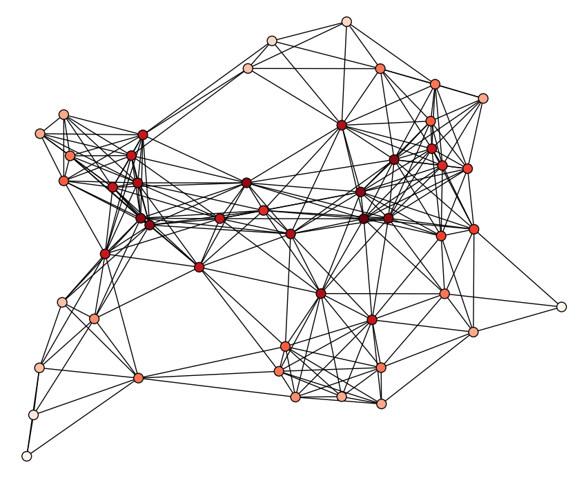
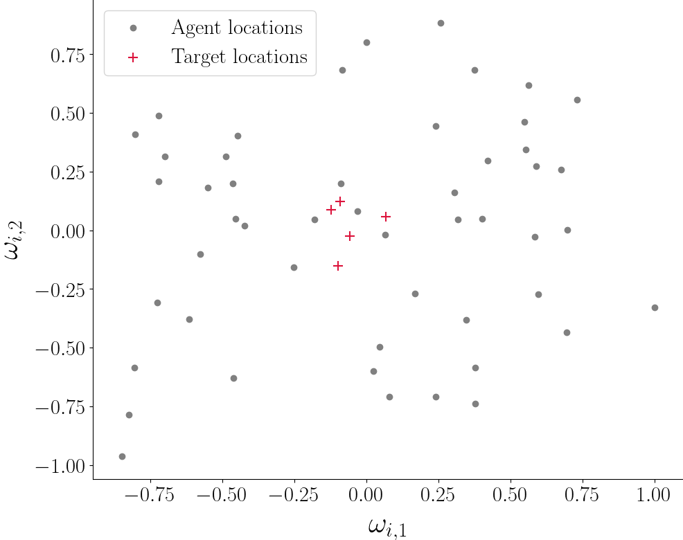
where is a random variable that represents a noisy distance metric, and is a stacking of the vectors . Note that (114) is indeed non-convex, but it is not globally -smooth for any However, we still find this problem is valuable to test our methods. Denote the true targets as for all these are used to generate for all and by computing where is drawn from a normal distribution with mean 0 and variance For all of our experiments we set We simulate agent connectivity by randomly generating agents in grid and creating an edge between agents if the Euclidean distance between them is less than or equal to 0.3. Each coordinate in the targets is drawn independently from a normal distribution with mean 0 and variance 0.1. Figure 2 shows the connectivity of the agents, as well as an example of target locations.
 |
 |
 |
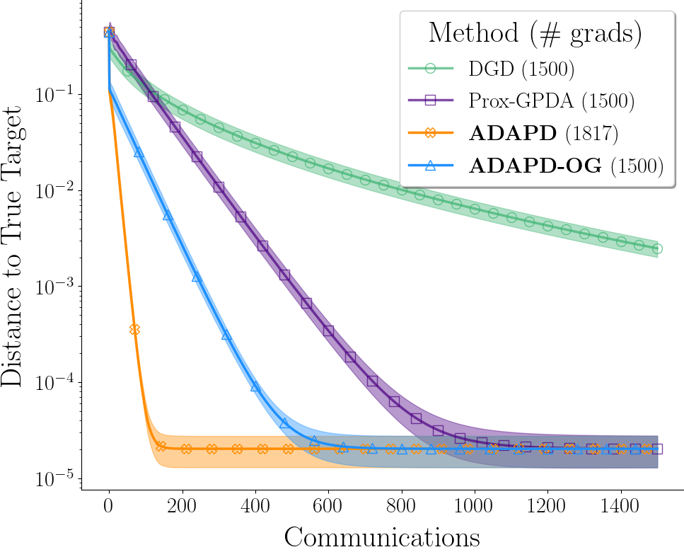 |
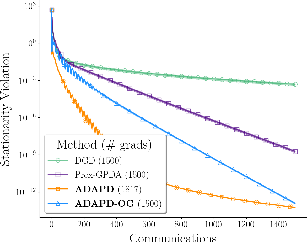
For this example, is chosen to be the Laplacian-based constant edge weight matrix from (4). We randomly generate targets and limit the communications to be 1,500 for all algorithm runs, with all methods starting from the same initial point. Since the targets are randomly generated for each experiment, we perform 10 independent trials and plot the mean results, with an associated 95% confidence interval.
Figure 2 shows that in terms of stationarity violation, ADAPD is superior to DGD and Prox-GPDA. Using only 20% more gradient computations on each agent, ADAPD is able to both solve the localization problem and find the true targets with fewer communications than the other methods. Additionally, ADAPD-OG utilizes the same number of gradient computations and neighbor communications as Prox-GPDA and DGD, but still performs better.
IV-C Convolutional Neural Networks
For these experiments, we fix agents and use a ring-structured graph where self-weighting and neighbor weighting is set to be . We train the models on a cluster of 8 NVIDIA Tesla V100 GPUs, where each GPU represents an agent. PyTorch is used in the training of the models and OpenMPI is used to perform the neighbor communication of the neural network weights. All experiments are performed with 10 different initial starting points. We report the average results, as well as a 95% confidence interval taken over the 10 trials.
IV-C1 MNIST
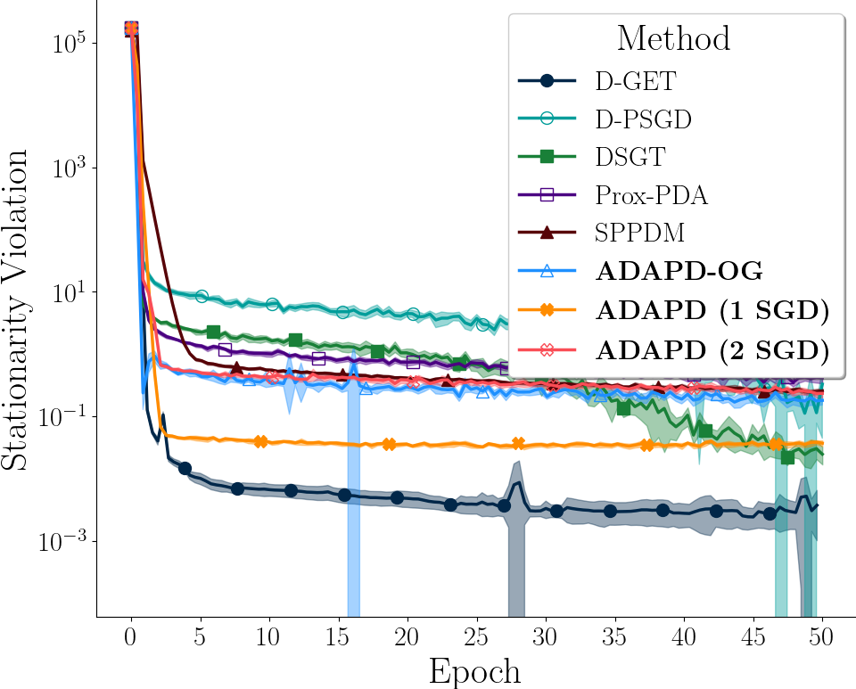
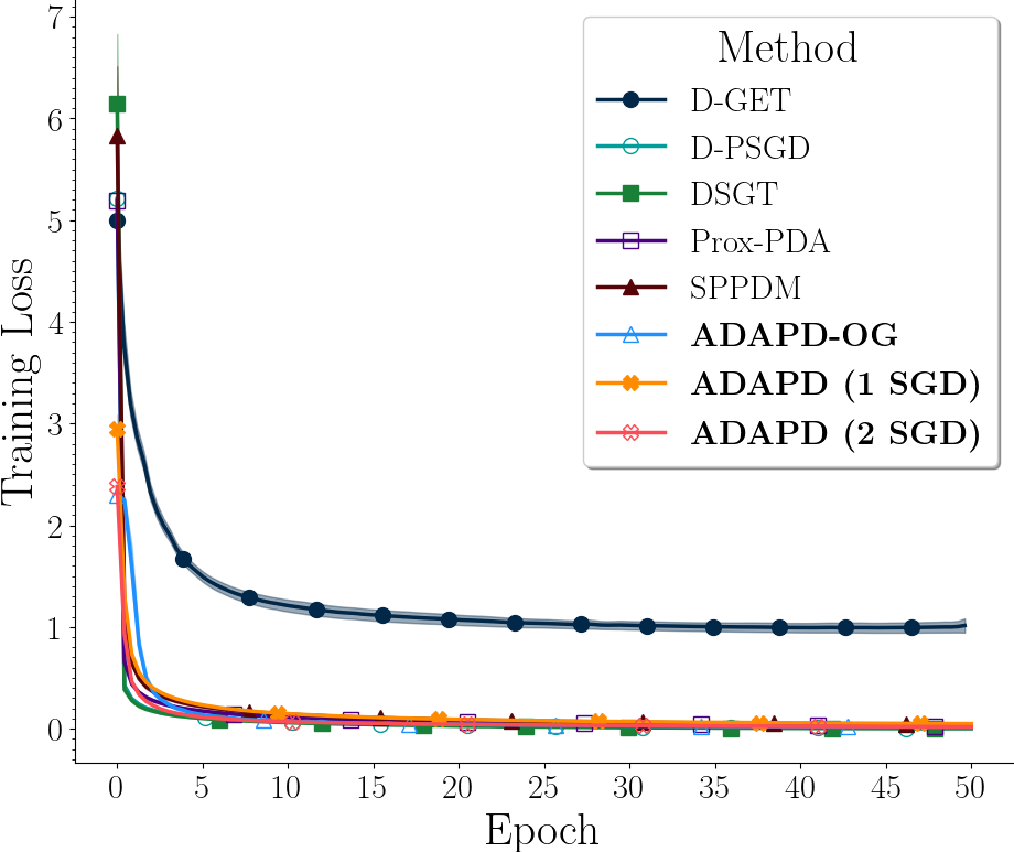
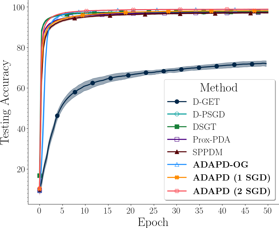
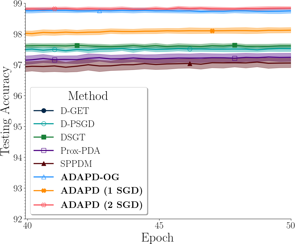
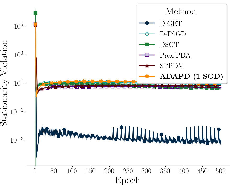
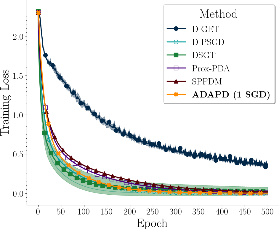
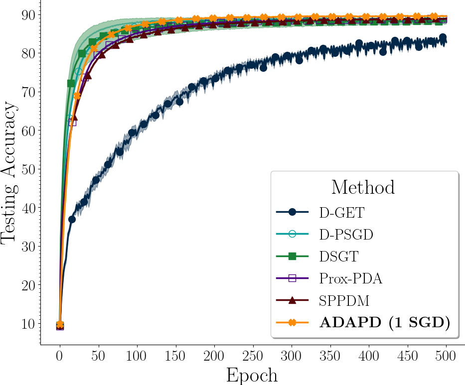
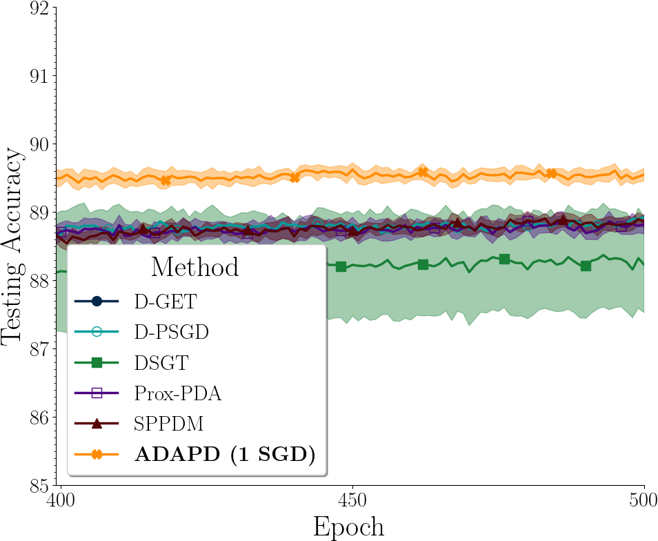
The first Convolutional Neural Network (CNN) experiment we perform is training LeNet [52] on the MNIST dataset. We make the activation function for each layer the hyperbolic tangent function to ensure smoothness of the local objective functions. Since methods like DSGT [32] and D-GET [11] require multiple neighbor communications during each update, we instead fix the number of epochs for this experiment to 50 and fix the mini-batch size to 64 for all methods. We randomly generate 10 sets of initial points for the agents and report the average of all relevant metrics, as well as a 95% confidence interval. For ADAPD and ADAPD-OG, we simply replace the full gradient computation by a stochastic gradient during each local agent update. It is worth noting that neither ADAPD, nor Prox-PDA, have theoretical convergence guarantees in this experimental setting. Nonetheless, we see impressive results for this problem and thus include it. To see the effect of stochasticity here, we run the ADAPD in Alg. 1 by computing both one and two stochastic gradients during line 3. For Prox-PDA, we compute one stochastic gradient step. Similar to [2], we report the stationarity violation for all methods, as well as the training loss and testing accuracy using the average of the local agent’s weights444Similar results for both the MNIST and CIFAR-10 image classification problems are observed if the local weights are used to compute the training loss and testing accuracy.. In practice, this is not feasible due to the decentralized communication pattern, however, an average model can be obtained after all local training has been done by performing many neighbor communication rounds [12]. Note that the training loss reported here is not scaled by to facilitate a fair comparison with standard CNN training methods (i.e. centralized training).
 |
 |
 |
 |
Additionally, we report the wall-clock time taken to reach and stay above 97% testing accuracy for the MNIST image classification problem in Table I. This value comes from selecting the highest whole number of testing accuracy that most methods exceed. D-GET does not achieve this accuracy in the alloted amount of epochs. The “Samples” column indicates the amount of data visited by each agent to achieve the 97% testing accuracy and the “Communications” column indicates the corresponding number of communications performed by each agent (for D-GET, these values are simply the total numbers used during training). We also include each method’s highest testing accuracy in the last column.
| Method | To reach 97% testing accuracy | Highest accuracy (%) | ||
|---|---|---|---|---|
| Time (s) | Samples | Communications | ||
| D-GET | ✗ | 376,524 | 4,096 | 72.17 |
| D-PSGD | 31.56 | 92,800 | 1,450 | 97.53 |
| DSGT | 26.78 | 73,600 | 2,300 | 97.64 |
| Prox-PDA | 80.99 | 227,200 | 3,550 | 97.25 |
| SPPDM | 116.73 | 326,400 | 5,100 | 97.09 |
| ADAPD-OG | 16.35 | 48,000 | 750 | 98.77 |
| ADAPD (1 SGD) | 74.2 | 121,600 | 1,900 | 98.12 |
| ADAPD (2 SGD) | 47.5 | 83,200 | 650 | 98.85 |
While D-GET is able to achieve the lowest stationarity violation, the training loss and testing accuracy indicate it does not converge to a solution that solves the classification problem well. Figure 3 and Table I show that both ADAPD and ADAPD-OG outperform competitors in terms of testing accuracy, suggesting that ADAPD is able to find a solution that generalizes better than other methods. Additionally, Table I shows that ADAPD (with 2 SGD steps) and ADAPD-OG require far fewer communications to achieve a high testing accuracy. In a network setting where communication time dominates the computation time, ADAPD and its variants can outperform the competitors.
IV-C2 CIFAR-10
The second CNN experiment we perform is training the ALL-CNN model [53] on the CIFAR-10 dataset [54]. We add batch normalization after every ReLU activation function and perform no data augmentation prior to training. For these experiments, we fix the mini-batch size to 128 for all methods and limit the number of updates so that each method runs for 500 epochs. We only use the ADAPD algorithm with 1 stochastic gradient step for these experiments, but we tune the dual step-size in (25) and (26). In Figure 4, we report the same metrics as in the MNIST experiment.
 |
 |
 |
 |
| Method | To reach 88% testing accuracy | Highest accuracy (%) | ||
|---|---|---|---|---|
| Time (s) | Samples | Communications | ||
| D-GET | ✗ | 3,125,006 | 35,530 | 84.16 |
| D-PSGD | 651.88 | 1,011,200 | 7,900 | 88.92 |
| DSGT | 1,900.23 | 2,348,800 | 36,700 | 88.37 |
| Prox-PDA | 1,025.57 | 1,523,200 | 11,900 | 88.88 |
| SPPDM | 1,395.84 | 1,708,800 | 13,350 | 88.91 |
| ADAPD (1 SGD) | 870.11 | 806,400 | 6,300 | 89.62 |
Similar to the MNIST image classification problem, we report the wall-clock time taken to reach and stay above 88% testing accuracy in Table II. In terms of stationarity, all methods besides D-GET struggle. However, ADAPD performs better than the competitors in terms of testing accuracy (see Figure 4 and Table II). Similar to the MNIST results, this suggests that ADAPD is able to find a solution to the image classification problem that generalizes better than the competitors. Additionally, ADAPD greatly saves on the number of data samples and communications necessary to achieve a high testing accuracy.
V Conclusion
In this work, we presented ADAPD: A DecentrAlized Primal-Dual framework for solving non-convex and smooth consensus optimization problems over a network of agents. Two variants to ADAPD are presented, the ADAPD-OG (One Gradient) and the ADAPD-MC (Multiple Communications). We demonstrated that ADAPD and ADAPD-OG achieves communication complexity to find an -stationary point and showed this can be reduced to when the MC variant is used; this is optimal for the class of smooth, non-convex, decentralized consensus problems considered in this work. Finally, we presented four numerical experiments that validate our claim that ADAPD outperforms other state-of-the-art decentralized methods. Future research topics would be extending the theoretical guarantees of ADAPD-OG to the stochastic case and demonstrating convergence in a time-varying/asynchronous setting of ADAPD and its variants.
References
- [1] B. McMahan, E. Moore, D. Ramage, S. Hampson, and B. A. y. Arcas, “Communication-Efficient Learning of Deep Networks from Decentralized Data,” in Proceedings of the 20th International Conference on Artificial Intelligence and Statistics (A. Singh and J. Zhu, eds.), vol. 54 of Proceedings of Machine Learning Research, pp. 1273–1282, PMLR, 20–22 Apr 2017.
- [2] X. Lian, C. Zhang, H. Zhang, C.-J. Hsieh, W. Zhang, and J. Liu, “Can decentralized algorithms outperform centralized algorithms? a case study for decentralized parallel stochastic gradient descent,” in Advances in Neural Information Processing Systems (I. Guyon, U. V. Luxburg, S. Bengio, H. Wallach, R. Fergus, S. Vishwanathan, and R. Garnett, eds.), vol. 30, pp. 5330–5340, Curran Associates, Inc., 2017.
- [3] X. Liang, A. M. Javid, M. Skoglund, and S. Chatterjee, “Asynchrounous decentralized learning of a neural network,” in ICASSP 2020 - 2020 IEEE International Conference on Acoustics, Speech and Signal Processing (ICASSP), pp. 3947–3951, 2020.
- [4] M. Hong, D. Hajinezhad, and M.-M. Zhao, “Prox-PDA: The proximal primal-dual algorithm for fast distributed nonconvex optimization and learning over networks,” in Proceedings of the 34th International Conference on Machine Learning (D. Precup and Y. W. Teh, eds.), vol. 70 of Proceedings of Machine Learning Research, (International Convention Centre, Sydney, Australia), pp. 1529–1538, PMLR, 06–11 Aug 2017.
- [5] J. Chen and A. H. Sayed, “Diffusion adaptation strategies for distributed optimization and learning over networks,” IEEE Transactions on Signal Processing, vol. 60, no. 8, pp. 4289–4305, 2012.
- [6] W. Shi, Q. Ling, G. Wu, and W. Yin, “Extra: An exact first-order algorithm for decentralized consensus optimization,” SIAM Journal on Optimization, vol. 25, pp. 944 – 966, 2015.
- [7] P. D. Lorenzo and G. Scutari, “Next: In-network nonconvex optimization,” IEEE Transactions on Signal and Information Processing over Networks, vol. 2, no. 2, pp. 120–136, 2016.
- [8] P. Abichandani, H. Y. Benson, and M. Kam, “Decentralized multi-vehicle path coordination under communication constraints,” in 2011 IEEE/RSJ International Conference on Intelligent Robots and Systems, pp. 2306–2313, 2011.
- [9] K. Scaman, F. Bach, S. Bubeck, Y. T. Lee, and L. Massoulié, “Optimal algorithms for smooth and strongly convex distributed optimization in networks,” in Proceedings of the 34th International Conference on Machine Learning (D. Precup and Y. W. Teh, eds.), vol. 70 of Proceedings of Machine Learning Research, (International Convention Centre, Sydney, Australia), pp. 3027–3036, PMLR, 06–11 Aug 2017.
- [10] K. Yuan, Q. Ling, and W. Yin, “On the convergence of decentralized gradient descent,” SIAM Journal on Optimization, vol. 26, pp. 1835 – 1854, 2016.
- [11] H. Sun, S. Lu, and M. Hong, “Improving the sample and communication complexity for decentralized non-convex optimization: Joint gradient estimation and tracking,” in Proceedings of the 37th International Conference on Machine Learning (H. D. III and A. Singh, eds.), vol. 119 of Proceedings of Machine Learning Research, (Virtual), pp. 9217–9228, PMLR, 13–18 Jul 2020.
- [12] L. Xiao and S. Boyd, “Fast linear iterations for distributed averaging,” Systems and Control Letters, vol. 53, no. 1, pp. 65–78, 2004.
- [13] E. Wei and A. Ozdaglar, “On the o(1/k) convergence of asynchronous distributed alternating direction method of multipliers,” in 2013 IEEE Global Conference on Signal and Information Processing, pp. 551–554, 2013.
- [14] K. Wang, I. Shen, C. Huang, C.-H. Wu, Y. Dong, and A. Kanakia, “Microsoft academic graph: when experts are not enough,” Quantitative Science Studies, vol. 1, pp. 396–413, February 2020.
- [15] Y. Arjevani, J. Bruna, B. Can, M. Gurbuzbalaban, S. Jegelka, and H. Lin, “Ideal: Inexact decentralized accelerated augmented lagrangian method,” in Advances in Neural Information Processing Systems (H. Larochelle, M. Ranzato, R. Hadsell, M. F. Balcan, and H. Lin, eds.), vol. 33, pp. 20648–20659, Curran Associates, Inc., 2020.
- [16] W. Shi, Q. Ling, K. Yuan, G. Wu, and W. Yin, “On the linear convergence of the admm in decentralized consensus optimization,” IEEE Transactions on Signal Processing, vol. 62, no. 7, pp. 1750–1761, 2014.
- [17] S. Boyd, N. Parikh, E. Chu, B. Peleato, and J. Eckstein, “Distributed optimization and statistical learning via the alternating direction method of multipliers,” vol. 3, no. 1, 2011.
- [18] Y. Wang, W. Yin, and J. Zeng, “Global convergence of admm in nonconvex nonsmooth optimization,” Journal of Scientific Computing, vol. 78, no. 1, pp. 29–63, 2019.
- [19] H. Sun and M. Hong, “Distributed non-convex first-order optimization and information processing: Lower complexity bounds and rate optimal algorithms,” IEEE Transactions on Signal Processing, vol. 67, no. 22, pp. 5912–5928, 2019.
- [20] D. P. Bertsekas and J. N. Tsitsiklis, Parallel and Distributed Computation: Numerical Methods. USA: Prentice-Hall, Inc., 1989.
- [21] X. Li, K. Huang, W. Yang, S. Wang, and Z. Zhang, “On the convergence of fedavg on non-iid data,” in International Conference on Learning Representations, 2020.
- [22] A. Nedic and A. Ozdaglar, “Distributed subgradient methods for multi-agent optimization,” IEEE Transactions on Automatic Control, vol. 54, pp. 48 – 61, 2009.
- [23] A. S. Berahas, R. Bollapragada, N. S. Keskar, and E. Wei, “Balancing communication and computation in distributed optimization,” IEEE Transactions on Automatic Control, vol. 64, no. 8, pp. 3141–3155, 2019.
- [24] G. Qu and N. Li, “Accelerated distributed nesterov gradient descent,” IEEE Transactions on Automatic Control, 2019.
- [25] C. A. Uribe, S. Lee, A. Gasnikov, and A. Nedić, “A dual approach for optimal algorithms in distributed optimization over networks,” Optimization Methods and Software, vol. 36, no. 1, pp. 171–210, 2021.
- [26] F. Mansoori and E. Wei, “Flexpd: A flexible framework of first-order primal-dual algorithms for distributed optimization,” IEEE Transactions on Signal Processing, vol. 69, pp. 3500–3512, 2021.
- [27] J. Zeng and W. Yin, “On nonconvex decentralized gradient descent,” IEEE Transactions on Signal Processing, vol. 66, pp. 2834 – 2848, 2018.
- [28] M. Hong, Z.-Q. Luo, and M. Razaviyayn, “Convergence analysis of alternating direction method of multipliers for a family of nonconvex problems,” SIAM Journal on Optimization, vol. 26, no. 1, pp. 337–364, 2016.
- [29] G. Scutari and Y. Sun, “Distributed nonconvex constrained optimization over time-varying digraphs,” Mathematical Programming, vol. 176, no. 1, pp. 497–544, 2019.
- [30] W. Auzinger and J. M. Melenk, “Iterative solution of large linear systems,” TU Wien, Lecture Notes, 2011.
- [31] H. Tang, X. Lian, M. Yan, C. Zhang, and J. Liu, “: Decentralized training over decentralized data,” in Proceedings of the 35th International Conference on Machine Learning (J. Dy and A. Krause, eds.), vol. 80 of Proceedings of Machine Learning Research, (Stockholmsmässan, Stockholm Sweden), pp. 4848–4856, PMLR, 10–15 Jul 2018.
- [32] J. Zhang and K. You, “Decentralized stochastic gradient tracking for non-convex empirical risk minimization,” arXiv preprint arXiv:1909.02712, 2020.
- [33] L. M. Nguyen, J. Liu, K. Scheinberg, and M. Takáč, “SARAH: A novel method for machine learning problems using stochastic recursive gradient,” in Proceedings of the 34th International Conference on Machine Learning (D. Precup and Y. W. Teh, eds.), vol. 70 of Proceedings of Machine Learning Research, (International Convention Centre, Sydney, Australia), pp. 2613–2621, PMLR, 06–11 Aug 2017.
- [34] A. Koloskova, T. Lin, and S. U. Stich, “An improved analysis of gradient tracking for decentralized machine learning,” in Advances in Neural Information Processing Systems (A. Beygelzimer, Y. Dauphin, P. Liang, and J. W. Vaughan, eds.), 2021.
- [35] R. Xin, U. A. Khan, and S. Kar, “Fast decentralized nonconvex finite-sum optimization with recursive variance reduction,” SIAM Journal on Optimization, vol. 32, no. 1, pp. 1–28, 2022.
- [36] X. Yi, S. Zhang, T. Yang, T. Chai, and K. H. Johansson, “A primal-dual sgd algorithm for distributed nonconvex optimization,” arXiv preprint arXiv:2006.03474, 2020.
- [37] Z. Wang, J. Zhang, T.-H. Chang, J. Li, and Z.-Q. Luo, “Distributed stochastic consensus optimization with momentum for nonconvex nonsmooth problems,” IEEE Transactions on Signal Processing, vol. 69, pp. 4486–4501, 2021.
- [38] X. Lian, W. Zhang, C. Zhang, and J. Liu, “Asynchronous decentralized parallel stochastic gradient descent,” Proceedings of the 35th International Conference on Machine Learning, vol. 80, pp. 3043–3052, 2018.
- [39] T. Wu, K. Yuan, Q. Ling, W. Yin, and A. Sayed, “Decentralized consensus optimization with asynchrony and delays,” IEEE Transactions on Signal and Information Processing over Networks, vol. 4, pp. 293 – 307, 2017.
- [40] J. Zhang and K. You, “Fully asynchronous distributed optimization with linear convergence in directed networks,” arXiv preprint arXiv:1901.08215, 2021, 1901.08215.
- [41] M. Hong, “A distributed, asynchronous, and incremental algorithm for nonconvex optimization: An admm approach,” IEEE Transactions on Control of Network Systems, vol. 5, no. 3, pp. 935–945, 2018.
- [42] S. Pu, W. Shi, J. Xu, and A. Nedić, “Push-pull gradient methods for distributed optimization in networks,” IEEE Transactions on Automatic Control, vol. 66, no. 1, pp. 1–16, 2021.
- [43] A. Nedic, A. Olshevsky, and W. Shi, “Achieving geometric convergence for distributed optimization over time-varying graphs,” SIAM Journal on Optimization, vol. 27, pp. 2597 – 2633, 2017.
- [44] J. Eckstein and W. Yao, “Relative-error approximate versions of douglas–rachford splitting and special cases of the admm,” Mathematical Programming, vol. 170, no. 2, pp. 417–444, 2018.
- [45] S. Kumar, K. Rajawat, and D. P. Palomar, “Distributed inexact successive convex approximation admm: Analysis-part i,” 2019, 1907.08969.
- [46] X. Zhang, M. Hong, S. Dhople, W. Yin, and Y. Liu, “Fedpd: A federated learning framework with adaptivity to non-iid data,” IEEE Transactions on Signal Processing, vol. 69, pp. 6055–6070, 2021.
- [47] J. Liu and A. S. Morse, “Accelerated linear iterations for distributed averaging,” Annual Reviews in Control, vol. 35, no. 2, pp. 160–165, 2011.
- [48] H. Ye, Z. Zhou, L. Luo, and T. Zhang, “Decentralized accelerated proximal gradient descent,” in Advances in Neural Information Processing Systems (H. Larochelle, M. Ranzato, R. Hadsell, M. F. Balcan, and H. Lin, eds.), vol. 33, pp. 18308–18317, Curran Associates, Inc., 2020.
- [49] A. Beck and M. Teboulle, “A fast iterative shrinkage-thresholding algorithm with application to wavelet-based image deblurring,” in 2009 IEEE International Conference on Acoustics, Speech and Signal Processing, pp. 693–696, 2009.
- [50] C.-C. Chang and C.-J. Lin, “LIBSVM: A library for support vector machines,” ACM Transactions on Intelligent Systems and Technology, vol. 2, pp. 27:1–27:27, 2011. Software available at http://www.csie.ntu.edu.tw/~cjlin/libsvm.
- [51] D. Dua and C. Graff, “Uci machine learning repository,” 2017.
- [52] Y. Lecun, L. Bottou, Y. Bengio, and P. Haffner, “Gradient-based learning applied to document recognition,” Proceedings of the IEEE, vol. 86, no. 11, pp. 2278–2324, 1998.
- [53] J. T. Springenberg, A. Dosovitskiy, T. Brox, and M. Riedmiller, “Striving for simplicity: The all convolutional net,” 2015, 1412.6806.
- [54] A. Krizhevsky, “Learning multiple layers of features from tiny images,” tech. rep., 2009.
Appendix A Supporting Lemmas and proofs for the Chebyshev acceleration
[cheby]
Appendix B On the equivalence between Prox-PDA [4] and distributed ADMM [16]
Here, we show that the distributed ADMM algorithm [16], which uses edge-based constraints to enforce consensus (see (3) in [16]), can reduce to the Prox-PDA method in [4]. Under the assumption of (the signed Laplacian of ), Prox-PDA performs global updates:
| (115) |
where . Choosing (the unsigned Laplacian of ), we have
Multiplying both sides of the update in (115) by , letting , and dropping the term from (B) (as the is about in (115)) results in (10) from [16]. Hence, the two algorithms are equivalent. As a result, the distributed ADMM updates from [16] converge in the non-convex case by the convergence of Prox-PDA [4].
Appendix C Supporting Lemmas and proofs for ADAPD
[dualbound]
The next three Lemmas serve as building blocks to prove Lemma III-A.
Lemma 1
If (28) is satisfied and , then
| (117) |
Lemma 2
The partial gradient is -Lipschitz continuous about for any . Further, for all we have
| (118) |
Proof Compute
where we have used the compatibility of the 2-norm and the Frobenius norm and Assumption 1(iv). Hence, it holds
Rearranging terms gives the desired result.
Lemma 3
For all the followings hold:
| (119) | |||
| (120) |
Proof By the update (25), we have
for all Hence, (119) holds. Similarly, by the update (26), we have
for all Thus (120) holds, and we complete the proof.
[buildLyapunov]
[inexactproofs]
Appendix D Supporting Lemmas and proofs for ADAPD-OG
We begin the convergence analysis with showing the change in the augmented Lagrangian function value between two consecutive iterations.
Lemma 4
Provided that , we have
| (121) |
for all
[normal]lemma Let be obtained from Alg. 2 or equivalently by updates (31) and (24)-(26). If , then it holds for all ,
| (122) |
The proof follows from rewriting as
and using (121), (118), (119), and (120) to bound each of the terms on the right hand side of the equality.
[normal]lemma Under the assumptions of Lemma 4, it holds that for all ,
| (123) | ||||
| (124) |
where is defined in (33).
To prove (123), we have from (101) that
To prove (124), we start from (45) to have
| (125) | ||||
| (126) | ||||
| (127) | ||||
| (128) |
where the last inequality uses Assumption 1(iv). Now we notice that (36) still holds for ADAPD-OG. Hence by choosing we have for all from (19). Thus (41) still holds, and it together with (125) implies (124).
By (101), we have
| (130) |
We handle the left and right hand side separately. For the left hand side, we have
For the right hand side, we have
Combining like terms results in the right hand side of (129); further using the equality established in (130) completes the proof.
[normal]lemma Let be obtained from Alg. 2 or equivalently by updates (31), (24)-(26). If , then
| (131) |
for all where is a fixed constant that satisfies
By Lemmas 4 and (122), we have
Multiplying to both sides of (129) and adding it to the above inequality gives
Since the minimum eigenvalue of is in (6), it holds when . Furthermore, since for , we have by noticing
| (132) | ||||
| (133) |
Thus,
Combining like terms, simplifying
and noting that yields the desired result.
We now define a new Lyapunov function based on the results from Lemma 4. Fix used in (131) and define
| (134) |
Before showing that this Lyapunov function is lower bounded, we first demonstrate the relation between the Lyapunov function at two consecutive iterations. Using Lemma 4, for all , we have
| (135) |
which comes directly from adding and subtracting to the left hand side of (131), combining like terms, and using (134). We now show that has a finite lower bound via the following proposition.
[normal]proposition Under Assumptions 1 and 2, let be obtained from Alg. 2 or equivalently by (31) and (24)-(26). Choose and such that
| (136) |
Then the Lyapunov function (134) is uniformly lower bounded. More specifically, for all
| (137) |
where is defined in Assumption 2.
First, we have for all by the definition of in (134). Second, by the definition of in (11), we have for any integer number ,
| (138) | ||||
| (139) |
Thirdly, by (135) and the choice of and , it holds that
| (140) |
Now assume that there exists a such that Then (140) gives for all Hence, which contradicts (138). Therefore, we conclude that for all and complete the proof.
We are now in position to prove the convergence rate results of Alg. 2.
[normal]thm Under the same conditions assumed in Proposition 4, it holds that
| (141) |
where and
| (142) |
Summing up (135) from to and dividing by results in
By the choice of and , the defined in (142) is positive, and the above inequality implies the desired result.
[singlestep]
Appendix E Proofs of the complexity results
[complexity]