Synthesizing arbitrary dispersion relations in a modulated tilted optical lattice

Abstract

Dispersion relations are fundamental characteristics of the dynamics of quantum and wave systems. In this work we introduce a simple technique to generate arbitrary dispersion relations in a modulated tilted lattice. The technique is illustrated by important examples: the Dirac, Bogoliubov and Landau dispersion relations (the latter exhibiting the roton and the maxon). We show that adding a slow chirp to the lattice modulation allows one to reconstruct the dispersion relation from dynamical quantities. Finally, we generalize the technique to higher dimensions, and generate graphene-like Dirac points and flat bands in two dimensions.

I Introduction

Dispersion relations, connecting the energy to the momentum, $E=E(\boldsymbol{p})$, of a quantum particle, or the frequency to the wave number $\omega=\omega(\boldsymbol{k})$ of a wave, are a fundamental concept in many domains of physics. For example, relativistic particles are characterized by the Einstein’s dispersion relation $E^{2}=p^{2}c^{2}+m^{2}c^{4}$, crystalline solids by their bands $E=E(\boldsymbol{q})$ (with $\boldsymbol{q}$ the quasimomentum) and superfluidity by Landau’s dispersion relation presenting exotic features like the maxon and the roton [1, 2, 3]. Dispersion relations provide a great deal of information on the physics of a system.

Recent developments both in condensed matter and ultracold-atom systems have generated the concept of “quantum simulator”. Devising, for instance, a system displaying a given dispersion relation provides information on several aspects of the physics of other systems exhibiting the same dispersion relation. Ultracold atoms in optical lattices or trapped ions have proved to be one of the most clean and flexible systems in physics, both theoretically and experimentally. Optical lattices can mimic an almost perfect lattice (no phonons, controllable decoherence, etc.) and make it easy to create low-dimensional systems. Moreover, being formed by the interference of laser beams, they can be “engineered” in many ways, e.g one can create a wealth of different lattices. A few, non-exaustive, examples are Kagome [4], Lieb [5, 6, 7], quasiperiodic [8] and disordered lattices [9]. They can also be easily modulated in time, producing, notably, oscillating [10] or accelerated lattices [11, 12]. These properties make such systems an outstanding platform to the realization of analog quantum simulators. In many cases, one can construct a given Hamiltonian from its building blocks, e.g. Bose- and Fermi-Hubbard’s [13, 14, 15], Anderson’s [9, 8, 16, 17] and Dirac’s [18, 19, 20, 21, 22] Hamiltonians, bringing new light into many aspects of their physics, notably the Mott transition [14], the Anderson localization and transition [17, 23, 24, 25], Bloch oscillations and Wannier-Stark systems [11, 12], or the Klein tunneling [26, 27].

In the present work we present a simple one dimensional system able to “synthesize” almost any desired dispersion relation, that we illustrate with important examples. An original technique allowing the direct detection of these dispersion relations is also proposed. In the last part, we generalize the synthesis of dispersion relations to higher dimensions, illustrated by the generation of graphene-like Dirac cones and Lieb lattices (displaying a flat band) in 2D.

II Synthesizing dispersion relations in one-dimensional Wannier-Stark optical lattices

Our present model is based on the framework introduced in Ref. [21] and further developed in [22]. Ultracold atoms are placed in the interference pattern of counter-propagating laser beams which generates a sinusoidal potential, proportional to the atom-laser coupling, acting on on the center-of-mass degree of freedom of the atoms [28]. The atomic cloud density is assumed low enough that atomic interactions are negligible. We consider here a one-dimensional Wannier-Stark system consisting of a sinusoidal optical lattice to which a constant force $F$ is applied:

$$H=\frac{p^{2}}{2m}-V_{0}\cos\left(\frac{2\pi x}{a}\right)+Fx.$$

This Hamiltonian can obtained by placing ultracold atoms on an accelerated standing laser wave [11, 12, 29]  of wavelength $k_{L}$, hence $a=\pi/k_{L}$. The properties of such a system are well known [31, 32, 33, 34, 35, 36, 37]. In short, this system is invariant under discrete spatial translations corresponding to an integer multiple $n$ of the lattice step $a$ provided the energy is also shifted of $nFa=n\hbar\omega_{B}$ where $\omega_{B}\equiv Fa/\hbar$ is the so-called Bloch frequency. In the following, $n$ denotes the site index corresponding to potential minima localized at the position $x=na$. The symmetry of the system implies that the eigenfunctions (called Wannier-Stark states) are invariant under a translation of an integer number of lattice steps, i.e $\varphi_{n}^{(\ell)}(x)=\varphi_{0}^{(\ell)}(x-na)$, with the corresponding eigenenergies $E_{n}^{(\ell)}=E_{0}^{(\ell)}+n\hbar\omega_{B}$, thus forming (depending on parameters $V_{0}$ and $F$) different ladders (labeled by $\ell$) of levels separated by a step $\hbar\omega_{B}$ and characterized by a ground energy shift $E_{0}^{(\ell)}$. In what follows we will mainly consider potential parameters allowing two ladders $(\ell=g,e)$ of localized “ground” and “excited” eigenstates, that is, there are two states localized at each site $n$, $\varphi_{n}^{(g)}(x)$ and $\varphi_{n}^{(e)}(x)$, separated by an energy shift $\Delta=E_{0}^{(e)}-E_{0}^{(g)}$. Other eigenstates of $H$, localized or belonging to the continuum, are supposed to be irrelevant for the system’s dynamics, as explained below.

A convenient set of dimensionless units is obtained by measuring space in units of $a$, energy in units of the so-called atom’s recoil energy $E_{R}\equiv\hbar^{2}k_{L}^{2}/2m$$=\hbar\omega_{R}$ and time in units of $\omega_{R}^{-1}$ ($m$ is the atom’s mass). This leads to the dimensionless Hamiltonian

$$H_{0}=\frac{p^{2}}{2m^{*}}-V_{0}\cos\left(2\pi x\right)+\omega_{B}x$$ (1)

where $m^{*}=\pi^{2}/2$, $\omega_{B}$ is measured in $\omega_{R}$ units and Planck’s constant is $\hbar=1$.

Controllable dynamics can be induced in such systems by external modulations of the parameters $V_{0}$ (or $F$) at frequencies close to resonances, i.e close to $\Delta$ and to multiples of $\omega_{B}$. We thus add to $H_{0}$ a time-dependent potential

$$H_{1}(t)=f(t)V(x)$$ (2)

where $V(x)=\cos(2\pi x)$. Using this flexibility, the feasibility of models reproducing the Dirac equation (hence the Dirac dispersion relation) has been demonstrated in Refs. [21, 22].

The driving $f(t)$ has the general form

$$f(t)=\sum_{j,q}A_{j,q}\mathrm{e}^{\mathrm{i}j\omega_{B}t}\mathrm{e}^{\mathrm{i}q\Delta t}$$ (3)

with $j\in\mathds{Z}$, $q=0,\pm 1$ and $A_{j,q}=-A_{-j-q}^{*}$ (reality condition). For given integers $j$ the modulation resonantly couples states centered in sites separated by $j$ lattice steps. If $q=0$, one couples states $\varphi_{n}^{(\ell)}$ and $\varphi_{n+j}^{(\ell)}$ belonging to the same ladder $\ell$ (intraladder coupling). Interladder couplings between states $\varphi_{n}^{(g)}$ and $\varphi_{n+j}^{(e)}$ are obtained for $q=1$, or $\varphi_{n}^{(e)}$ and $\varphi_{n+j}^{(g)}$ for $q=-1$.

With the above provisions, the general solution for the system can be developed in the Wannier-Stark basis restricted to the subspace spanned by the ground and first excited ladder

$$\Psi(x,t)= \sum_{n}\left(c_{n}(t)\mathrm{e}^{-\mathrm{i}n\omega_{B}t}\varphi_{n}^{(g)}(x)\right.$$

$$\left.+d_{n}(t)\mathrm{e}^{-\mathrm{i}\left(n\omega_{B}+\Delta\right)t}\varphi_{n}^{(e)}(x)\right)$$ (4)

which holds if modulation amplitudes in $f(t)$ are low enough to avoid projection on other eigenstates of the Hamiltonian $H_{0}$.

Plugging this form into the Schrödinger equation for $H_{0}+H_{1}(t)$ one obtains a set of coupled differential equations for the amplitudes $c_{n}(t)$ and $d_{n}(t)$ (for details of this calculation, see the Appendix of Ref. [21]), which reads

$$\mathrm{i} \frac{d}{dt}\left(\begin{array}[]{c}c_{n}(t)\\ d_{n}(t)\end{array}\right)=\sum_{r\in\mathds{Z}}\left(\begin{array}[]{cc}T_{r}^{(gg)}&T_{r}^{(ge)}\\ T_{r}^{(eg)}&T_{r}^{(ee)}\end{array}\right)\left(\begin{array}[]{c}c_{n+r}(t)\\ d_{n+r}(t)\end{array}\right)$$ (11)

with coupling amplitudes between sites $n$ and $n+r$ 

$$T_{r}^{(gg)} =A_{r,0}\left\langle\varphi_{0}^{(g)}\right|V\left|\varphi_{r}^{(g)}\right\rangle$$

$$T_{r}^{(ee)} =A_{r,0}\left\langle\varphi_{0}^{(e)}\right|V\left|\varphi_{r}^{(e)}\right\rangle$$

$$T_{r}^{(ge)} =A_{r,1}\left\langle\varphi_{0}^{(g)}\right|V\left|\varphi_{r}^{(e)}\right\rangle$$

$$T_{r}^{(eg)} =A_{r,-1}\left\langle\varphi_{0}^{(e)}\right|V\left|\varphi_{r}^{(g)}\right\rangle.$$ (12)

In the momentum representation the corresponding amplitudes $\tilde{c}(k,t)=\sum_{n}c_{n}(t)\exp\left(-\mathrm{i}kn\right)$ (with analogous expressions for $d_{n}$) are governed by only two coupled equations

$$\mathrm{i} \frac{d}{dt}\left(\begin{array}[]{c}\tilde{c}(k,t)\\ \tilde{d}(k,t)\end{array}\right)=\left(\begin{array}[]{cc}F_{g}(k)&F(k)\\ F^{*}(k)&F_{e}(k)\end{array}\right)\left(\begin{array}[]{c}\tilde{c}(k,t)\\ \tilde{d}(k,t)\end{array}\right)$$ (19)

where

$$F_{\ell}(k)=\sum_{r=-\infty}^{\infty}T_{r}^{(\ell\ell)}\mathrm{e}^{\mathrm{i}kr}$$ (20)

with $\ell=\left\{g,e\right\}$, and

$$F(k)=\sum_{r=-\infty}^{\infty}T_{r}^{(ge)}\mathrm{e}^{\mathrm{i}kr}.$$ (21)

The functions $F_{\ell}(k)$ and $F(k)$ are Fourier series whose coefficients are proportional to the overlap integrals $T_{r}^{\ell\ell^{\prime}}$ of the wave functions centered at positions separated by $r$ sites but are controlled by the modulation coefficients $A_{j,q}$ [see Eqs. (12)].

Equations (19) define an effective Hamiltonian for a two-level-like system, whose eigenvalues determine the dispersion relation $\omega(k)$:

$$\left[\omega(k)-F_{g}(k)\right]\left[\omega(k)-F_{e}(k)\right]=\left|F(k)\right|^{2}.$$ (22)

This dispersion relation is $2\pi$-periodic and is conventionally defined in the interval $k\in\left[-\pi,\pi\right)$. Equation (22) is the basis of our technique for synthesizing dispersion relations: Specifying a given dispersion relation amounts to define the functions $F_{g}(k)$, $F_{e}(k)$ and $F(k)$ and, from Eqs. (20,21), to set conditions on the amplitudes $T_{r}^{(\ell,\ell^{\prime})}$, which allows one, with the help of Eqs. (12), to determine modulation parameters $A_{j,q}$ that must be used in the modulation term $H_{1}(t)$. Examples discussed in Sec. III illustrate how a desired dispersion relation can be obtained to a very good approximation.

III Applications

III.1 Dirac cone

A linear dispersion relation $\omega(k)=\pm c|k|$, also called Dirac cone (corresponding to a Dirac particle of zero mass), can be obtained from Eq. (22) with $F_{g}(k)=F_{e}(k)=0$ and $F(k)=c\left|k\right|$. This implies $T_{r}^{(g,g)}=T_{r}^{(e,e)}=0$, that is, no intraladder couplings, and interladder couplings given by Eq. (21). As the Fourier series of the function $|k|$ is

$$|k|=\left[\frac{\pi}{2}-\frac{4}{\pi}\sum_{r=1}^{\infty}\frac{\cos(rk)}{r^{2}}\right]$$

one must have

$$\sum_{r}T_{r}^{(g,e)}e^{\mathrm{i}kr}=c\left|k\right|=c\left[\frac{\pi}{2}-\frac{4}{\pi}\sum_{r}\frac{\cos(rk)}{r^{2}}\right]$$

which, from Eq. (12), gives

$$A_{0,1}\left\langle\varphi_{0}^{(g)}\right|V\left|\varphi_{0}^{(e)}\right\rangle=c\frac{\pi}{2}$$ (23)

and

$$A_{r,1}\left\langle\varphi_{0}^{(g)}\right|V\left|\varphi_{r}^{(e)}\right\rangle=\frac{c}{\pi r^{2}}\left[\cos(r\pi)-1\right]\qquad r>0.$$

The dispersion relation is thus synthesized by applying a modulation given by Eq. (3) with coefficients:

$$A_{r,1}= \frac{c\pi}{2}\left\langle\varphi_{0}^{(g)}\right|V\left|\varphi_{0}^{(e)}\right\rangle^{-1}\delta_{r,0}$$

$$+\frac{c}{\pi r^{2}}\left\{\cos(r\pi)-1\right\}\left\langle\varphi_{0}^{(g)}\right|V\left|\varphi_{r}^{(e)}\right\rangle^{-1}\left(1-\delta_{r0}\right).$$

Experimentally, this kind of modulation can be easily created by an arbitrary-wave generator. The overlap integrals $\left\langle\varphi_{0}^{(g)}\right|V\left|\varphi_{r}^{(e)}\right\rangle$ depend on the lattice parameters $V_{0}$ and $F$ and go to zero rather fast with the site distance $r$, implying that the modulation amplitude at higher frequencies must increase rapidly, eventually breaking the slow modulation condition implied by Eq. (4). Fortunately, for typical lattice parameters, keeping only $r\leq 3$ terms yet gives a rather good approximation of a Dirac cone, as shown Fig. 1 (top), except at the tip of the cone at $k=0$ which needs higher harmonics to be well reproduced.

A way to overcome this limitation is to include in Eq. (23) a frequency offset parameter $b$ such that $\omega(k)=\pm c\left(|k|+b\right)$, which is readily done by setting

$$A_{0,1}=c\left(b+\frac{\pi}{2}\right)\left\langle\varphi_{0}^{(g)}\right|V\left|\varphi_{0}^{(g)}\right\rangle^{-1}.$$

The parameter $b$ controls the gap between the two half-cones: If $b>0$ a gap is opened, and if $b<0$ one obtains two intersecting Dirac cones. Figure 1 (bottom) illustrates this case for $b=-1$ and shows perfect linear behavior in the vicinity of the Dirac points whose position $k=\pm b$ is controlled by the applied modulation. We have thus obtained flexible way to generate Dirac-cone-type dispersion relations, allowing one to open a gap or to merge the cones.

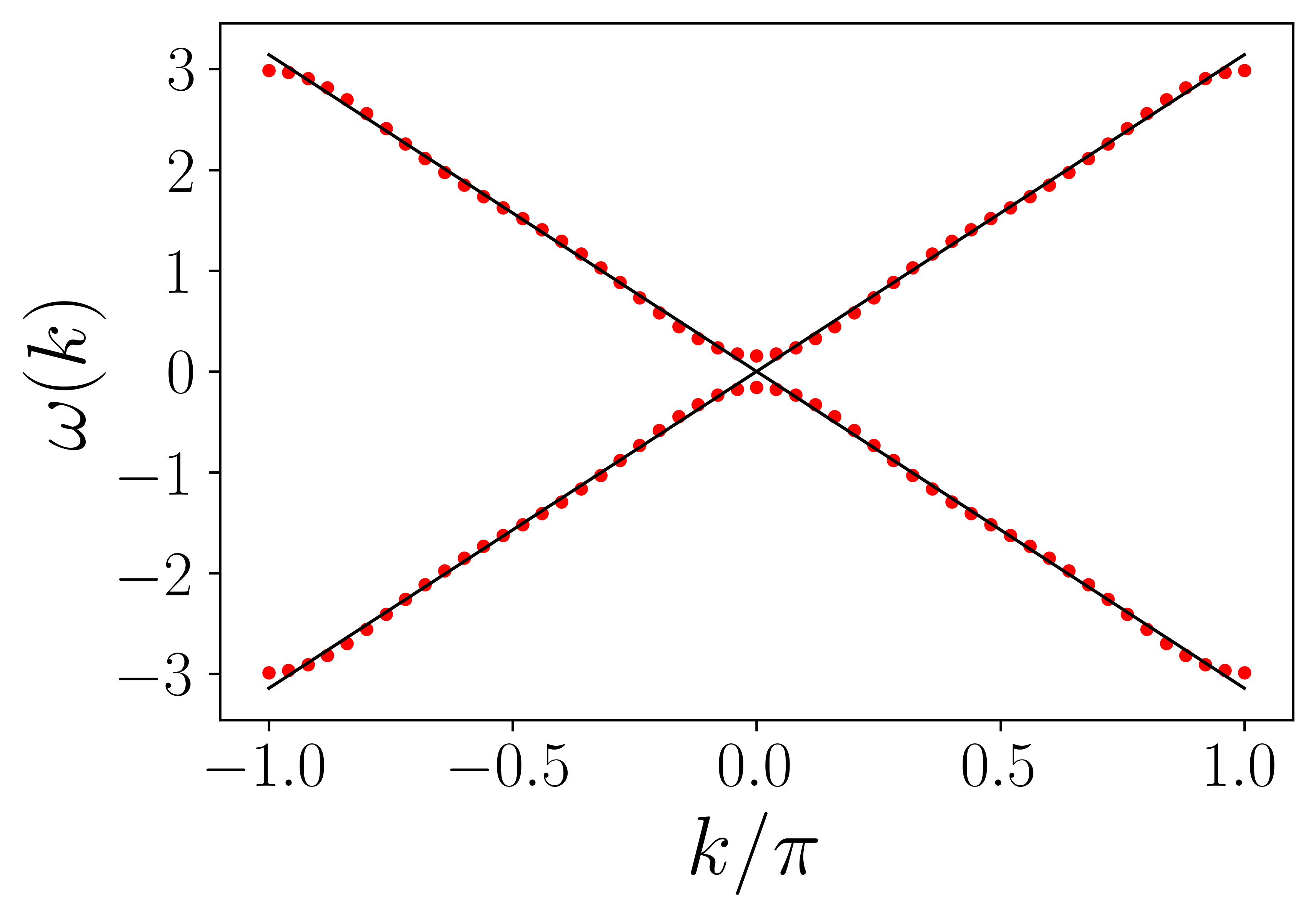
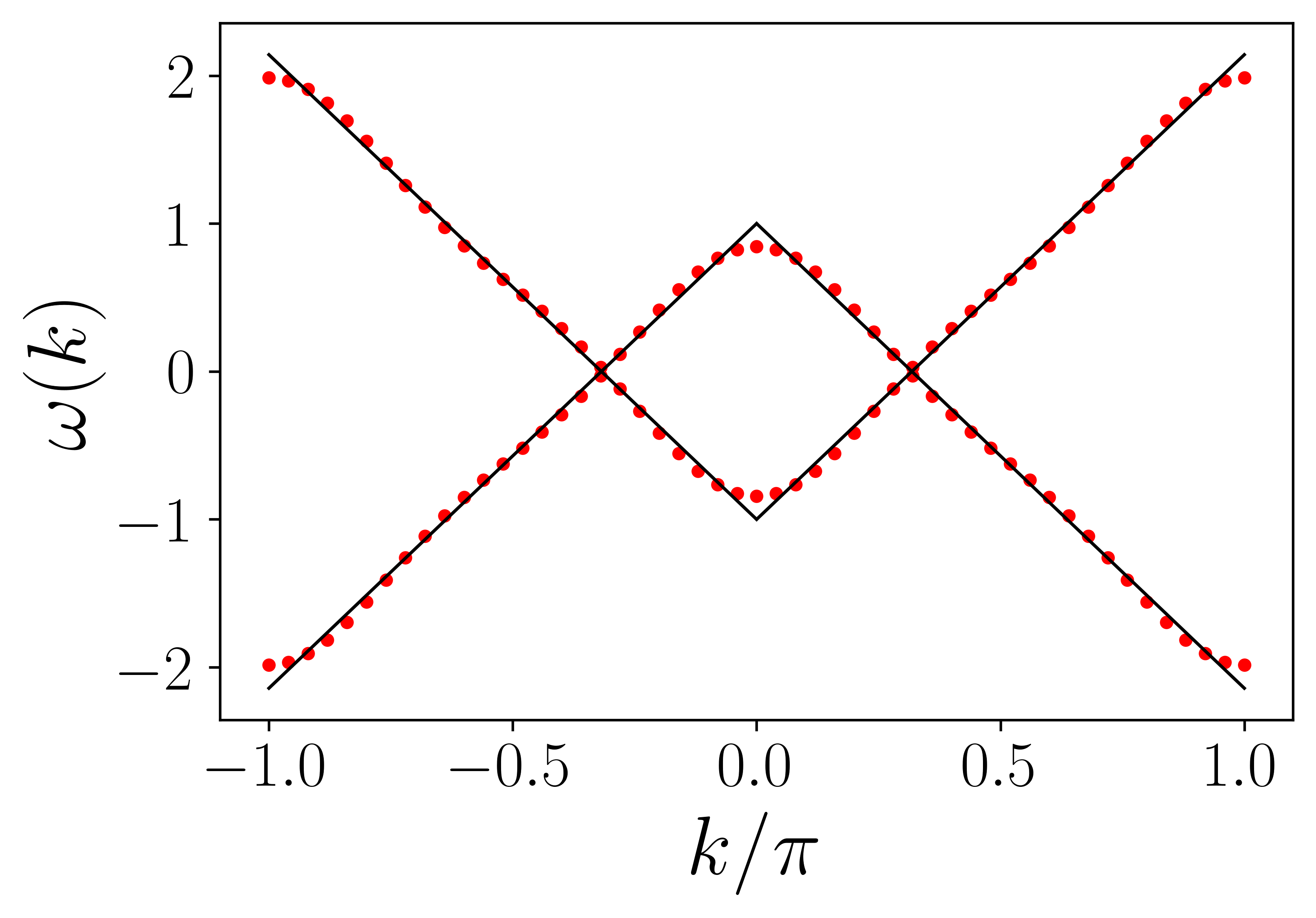
Figure 1: Linear dispersion relation. Top: Dirac cone ($c=1$); Bottom: intersecting Dirac cones ($c=1,b=-1$). Only terms $0\leq r\leq 3$ were kept in the Fourier series (red circles). The analytical expressions are shown for comparison (black solid lines).

III.2 The superfluid dispersion relation, the roton and the maxon

Superfluidity is a purely quantum behavior appearing notably in liquid Helium and quantum atomic gases. Its simplest mathematical treatment relies on the Bogoliubov correction to the mean-field Gross-Pitaevskii equation [39, 28, 3], which leads to the well-known Bogoliubov dispersion relation

$$\omega(k)=\sqrt{\frac{k^{2}}{2M}\left(\frac{\hbar^{2}k^{2}}{2M}+2gn\right)}$$ (24)

where $M$ is the atom mass, $g$ a parameter characterizing the binary atomic interaction in the Gross-Pitaevskii equation and $n$ the atomic density (the approximation is valid in the limit of low density and temperature). This dispersion is characterized by a “phononic”, i.e. linear $\omega(k)\propto k$ dependence at small $k$ $(k\ll\sqrt{gnM}/\hbar$) and a “free particle” part $\omega(k)\propto k^{2}$ at large $k$.

Following the same ideas as in the preceding section, Eq. (24) can be obtained from the general form of the dispersion relation with $F_{g}(k)=F_{e}(k)=0$ and

$$F(k)=c\left(\left|k\right|+\alpha k^{2}\right)$$ (25)

where $\alpha$ is an imaginary number ($\alpha=\mathrm{i}|\alpha|$), leading, through Eq. (22), to the desired dispersion

$$\omega(k)=c\sqrt{k^{2}\left(1+\left|\alpha\right|^{2}k^{2}\right)}$$ (26)

Beyond the Bogoliubov approach, phenomenological arguments by Landau [1] concerning the superfluidity of the strongly-interacting liquid ⁴He supported the existence in the dispersion relation of a minimum $\omega(k_{r})$ at some $k_{r}$, called the roton  which, by continuity, implies the existence of a maximum $\omega(k_{m})$ with $k_{m}<k_{r}$, called the maxon. Roton and maxon features have recently been observed experimentally using a Bose-Einstein condensate in a modulated flat lattice [41], in Erbium condensates with interactions controlled by Feshbach resonances [42, 43] and in acoustic metamaterials [44].

A dispersion relation presenting a roton and maxon can be synthesized by choosing $\alpha$ as a complex number, thus

$$\omega(k)=c\sqrt{k^{2}\left(1+\left(\alpha+\alpha^{*}\right)|k|+\left|\alpha\right|^{2}k^{2}\right)}.$$ (27)

Equation (21) then leads to

$$T_{r}^{ge}=A_{r,1}\left\langle\varphi_{0}^{g}\right|V\left|\varphi_{r}^{e}\right\rangle=\frac{c}{\pi}\intop_{0}^{\pi}\cos\left(rk\right)\left(\left|k\right|+\alpha k^{2}\right),$$

from which we obtain the modulation amplitudes

$$A_{r,1}=c\left(\frac{\pi}{2}+\alpha\frac{\pi^{2}}{3}\right)\left\langle\varphi_{0}^{(g)}\right|V\left|\varphi_{0}^{(e)}\right\rangle^{-1}\delta_{r0}+\frac{c}{\pi r^{2}}\left[(2\pi\alpha+1)\cos(r\pi)-1\right]\left\langle\varphi_{0}^{(g)}\right|V\left|\varphi_{r}^{(e)}\right\rangle^{-1}\left(1-\delta_{r0}\right).$$ (28)

The fact that $\left|A_{r,1}\right|\propto r^{-2}$ (for $r\neq 0$) implies that the series has a rather fast convergence, and thus only a few terms suffice to give a good approximation of the desired dispersion relation. Figure (2) shows the resulting Bogoliubov dispersion relation with the roton-maxon features obtained for $\alpha=-0.5+0.1\mathrm{i}$, compared to Eq. (27).

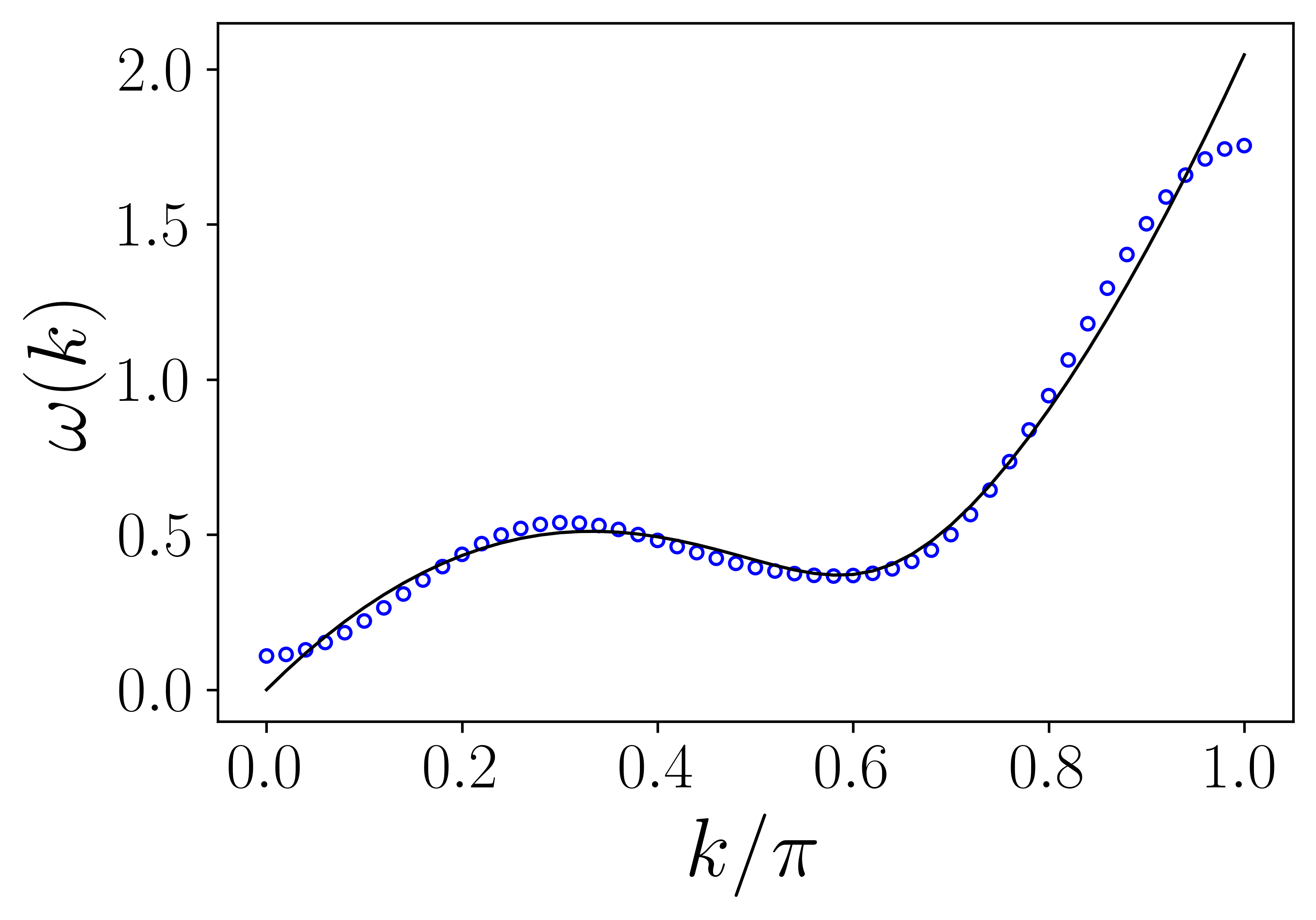
Figure 2: Synthetic dispersion relation displaying a maxon and a roton, generated by the Fourier series Eq. (28) (blue circles), restricted to $|r|\leq 3$, compared to Eq. (27) with parameters $c=1$ and $\alpha=-0.5+0.1\mathrm{i}$ (black solid line).

III.3 Scanning the dispersion relation

A natural question is, how to obtain experimental information on the shape of the dispersion relation? We show below that this can be done by preparing an initial wave packet and monitoring its average position $\left\langle X\right\rangle(t)$, in the modulated lattice while applying a slow phase chirp to the modulation Eq. (3); we thus use a generalized modulation form $\sum_{j}A_{j,q}\exp\left(\mathrm{i}\left[j\left(\omega_{B}t+\phi(t)\right)+q\Delta t\right]\right)$, where $\phi(t)$ is an arbitrary phase modulation. All the developments of Sec. II remain valid except that, for a slow variation of $\phi(t)$, the amplitudes become $A_{j,0}\exp\left(\mathrm{i}j\phi(t)\right).$ Equations (12) show that phase modulation $\phi(t)$ is then imprinted in the coupling coefficients $T_{r}$, which finally results in shifting $k\rightarrow k(t)=k+\phi(t)$ in Eqs. (20,21). Changing the phase $\phi$ turns out to be equivalent to change $k$ , resulting in slowly varying functions $F(k(t))$ and $F_{\ell}\left(k(t)\right)$ and thus $\omega\left(k(t)\right)$.

We illustrate this idea in the simple case of an intraladder model with only the ground ladder $\ell=0$ [i.e. $q=0$ in Eq. (2)]. In this case we have $\omega(k)=F_{g}\left[k+\phi(t)\right]$, and a slow linear chirp $\phi=\gamma t$ ($\gamma\ll\omega_{B}$) results in $\left\langle X\right\rangle(t)=\left.\omega(k)\right|_{k=k(t)}/\gamma$ (see appendix A). We choose here the example of an analytical dispersion relation

$$\omega(k)=a\left[1-\cos(2k)\right]+b\sin(2k)+c\sin k$$ (29)

which exhibits a roton-like behavior as shown in Fig. 3 (full black line). We performed a numerical simulation of the full Schrödinger equation corresponding to the Hamiltonian $H=H_{0}+H_{1}(t)$ (with a suitable choice of modulation parameters) with an initial Gaussian wave packet whose width in $k-$space is small compared to the extent of the dispersion relation (or more precisely to its typical length scale). The time evolution of the wave packet is then registered while the phase is linearly swept $\phi(t)=\gamma t$. The evolution of the mean position $\left\langle X\right\rangle(t)$ is shown in Fig. 3 (blue circles) and shows a good agreement with the analytical expression Eq. (29), validating our proposal.

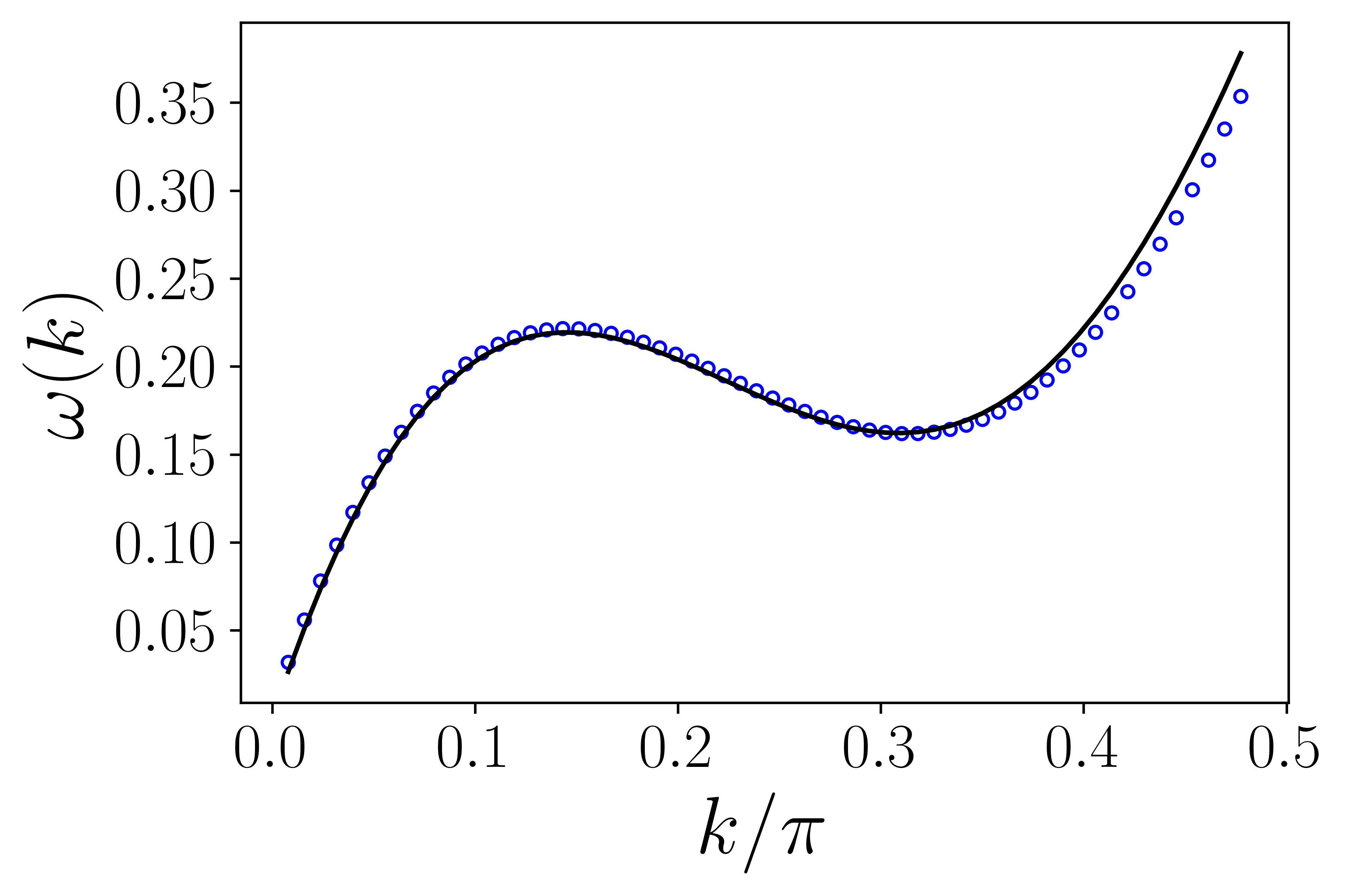
Figure 3: Detecting the dispersion relation. The solid black line dispersion relation is obtained from $\omega(k)=F_{g}\left[k+\phi(t)\right]$ with $F_{g}(k)=-0.81\left[1-\cos(2k)\right]-0.5\sin(2k)+2\sin k$ and $F_{e}=F=0$. The blue circles show the average wave packet position $\left\langle X\right\rangle(t)$ (with an adjusted vertical scale factor) and the chirp ratio $\gamma=\pi\times 10^{-4}\omega_{B}$.

IV Dispersion relations in two dimensions

The strategy developed in Sec. II can be generalized to higher dimensions. We give here two examples: the creation of 2D Dirac points and of a Lieb lattice dispersion relation with a flat band.

IV.1 Creating, moving and the merging of Dirac cones

Manipulation of Dirac points both in optical lattices [20] and crystals [46] is an active research subject. The creation of a 2D optical lattice simulating Dirac physics was discussed in Ref. [22]. In brief, the corresponding dispersion relations can be synthesized in a 2D modulated tilted lattice. Hamiltonian (2) is easily translated into 2D (the definition of the dimensionless units is analogous to the 1D case):

$$H_{0_{2D}}=\frac{p_{x}^{2}+p_{y}^{2}}{2m^{*}}-V_{0}\left(\cos(2\pi x)+\cos(2\pi y)\right)+\omega_{B}^{(x)}x+\omega_{B}^{(y)}y.$$ (30)

Since the above Hamiltonian is separable, all Wannier-Stark properties described in Sec. II trivially generalize to the present case. We consider only ground ladder eigenstates formed by the tensorial product $\varphi_{n}^{(x)}(x)\varphi_{m}^{(y)}(y)$ with $\varphi_{s}^{(i)}(x_{i})=\varphi_{0}^{(i)}(x_{i}-sx_{0_{i}})$, $i=\left\{x,y\right\},s=\left\{n,m\right\}$ with eigenenergies $E_{0}+n\omega_{B}^{(x)}+m\omega_{B}^{(y)}$ .

The controlled dynamics for Dirac system we are interested in is generated by adding a perturbation

$$H_{1_{2D}}(x,y,t)= \cos\left(\pi x\right)\left[V_{x}\mathrm{e}^{\mathrm{i}\left(2\omega_{B}^{(x)}t+\phi_{x}\right)}+\mathrm{c.c.}+V_{0}\right]$$

$$+ \left[V_{y}\cos\left(2\pi y\right)\mathrm{e}^{\mathrm{i}\left(\omega_{B}^{(y)}t+\phi_{y}\right)}+\mathrm{c.c.}\right]$$ (31)

depending on the arbitrary phases $\phi_{x,y}$. The general solution (restricted to the ground ladder) can be written, in analogy with Eq. (4),

$$\Psi(x,y,t)=\sum_{n,m}c_{n,m}(t)\varphi_{n}^{(x)}(x)\varphi_{m}^{(y)}(y).$$ (32)

Substituting the above solution in Schrödinger’s equation for the total Hamiltonian $H_{0_{2D}}+H_{1_{2D}}$, one obtains the following set of coupled equation (in the resonant approximation)

$$\mathrm{i}\frac{dc_{n,m}}{dt}= (-1)^{n}\left[T_{x}\mathrm{e}^{\mathrm{i}\phi_{x}}c_{n+2,m}+T_{x}\mathrm{e}^{-\mathrm{i}\phi_{x}}c_{n-2,m}+T_{0}c_{n,m}\right]$$

$$+T_{y}\mathrm{e}^{\mathrm{i}\phi_{y}}c_{n,m+1}+T_{y}\mathrm{e}^{-\mathrm{i}\phi_{y}}c_{n,m-1}$$

with couplings

$$T_{x} =V_{x}\left\langle\varphi_{0}^{(x)}\right|\cos\left(\pi x\right)\left|\varphi_{2}^{(x)}\right\rangle$$

$$T_{y} =V_{y}\left\langle\varphi_{0}^{(y)}\right|\cos\left(2\pi y\right)\left|\varphi_{1}^{(y)}\right\rangle$$

$$T_{0} =V_{0}\left\langle\varphi_{0}^{(x)}\right|\cos\left(\pi x\right)\left|\varphi_{0}^{(x)}\right\rangle$$

where the factor $\cos(\pi x)$ in Eq. (31) introduces a parity-dependent factor $(-1)^{n}$ which results in a system of two coupled sublattices corresponding to sites where $n$ is odd or even. In the reciprocal space $(k_{x},k_{y})$, we define two-dimensional Fourier amplitudes,

$$\tilde{c}(k_{x},k_{y},t)=\sum_{n\textrm{ even}}\sum_{m}c_{nm}(t)\mathrm{e}^{-\mathrm{i}nk_{x}}\mathrm{e}^{-\mathrm{i}mk_{y}}$$

for $n$ even, and, equivalently, for $n$ odd, $\tilde{d}(k_{x},k_{y},t)$. These amplitudes can be written as a two-component spinor $\left[\psi\right]=\left(\tilde{c}(k_{x},k_{y},t),\tilde{d}(k_{x},k_{y},t)\right){}^{\mathsf{T}}$. The Hamiltonian projected in the $k$-space turns out to be

$$\left[\begin{array}[]{cc}T_{0}+T_{x}\cos(2k_{x}+\phi_{x})&T_{y}\cos(k_{y}+\phi_{y})\\ T_{y}\cos(k_{y}+\phi_{y})&-T_{0}-T_{x}\cos(2k_{x}+\phi_{x})\end{array}\right]$$ (33)

for which the dispersion relation is

$$\omega(k_{x},k_{y})= \pm\left\{\left[T_{0}+T_{x}\cos(2k_{x}+\phi_{x})\right]^{2}\right.$$

$$\left.+\left[T_{y}\cos(k_{y}+\phi_{y})\right]^{2}\right\}^{1/2}.$$ (34)

In the $k_{x,y}\rightarrow 0$ limit, choosing $\phi_{x}=\phi_{y}=\pi/2$ and $T_{0}=0$, a Dirac equation (for a free particle) is obtained with the dispersion relation

$$\omega(k_{x},k_{y})=\pm\sqrt{4T_{x}^{2}k_{x}^{2}+T_{y}^{2}k_{y}^{2}}$$

which is a Dirac cone (anisotropic if $2T_{x}\neq T_{y}$).

Another interesting situation is obtained from Eq. (34) with $\phi_{x}=0$, $\phi_{y}=\pi/2$ and $T_{0}\neq 0$ . Then, the dispersion relation is, for small $k_{y}$

$$\omega(k_{x},k_{y})\approx\pm\sqrt{\left[T_{0}+T_{x}\cos(2k_{x})\right]^{2}+T_{y}^{2}k_{y}^{2}}$$ (35)

Depending on parameters $T_{0}$ and $T_{x}$, different structures are obtained (assuming here $T_{0}$ and $T_{x}$ of opposite sign without loss of generality). As shown in Fig. 4, when $\left|T_{0}\right|<\left|T_{x}\right|$, there are two Dirac cones centered at the positions $k_{y}=0$ and $k_{x}=\pm(1/2)\cos^{-1}\left(\left|T_{0}/T_{x}\right|\right)$. These cones moves towards each other as the value of $\left|T_{0}/T_{x}\right|$ increases, and finally coalesce when $T_{0}=-T_{x}$ giving a dispersion relation $\omega(k_{x},k_{y})\approx\pm\sqrt{4T_{x}^{2}k_{x}^{4}+T_{y}^{2}k_{y}^{2}}$ in the vicinity of the point $k_{x},k_{y}=0$, which is thus a hybrid point with a linear dependence in the $y$ direction (corresponding to a free Dirac particle, or phonon) and quadratic dependence in $x$ (corresponding to a free non-relativistic particle). A gap opens for $\left|T_{0}\right|>\left|T_{x}\right|$, potentially leading to topological effects.

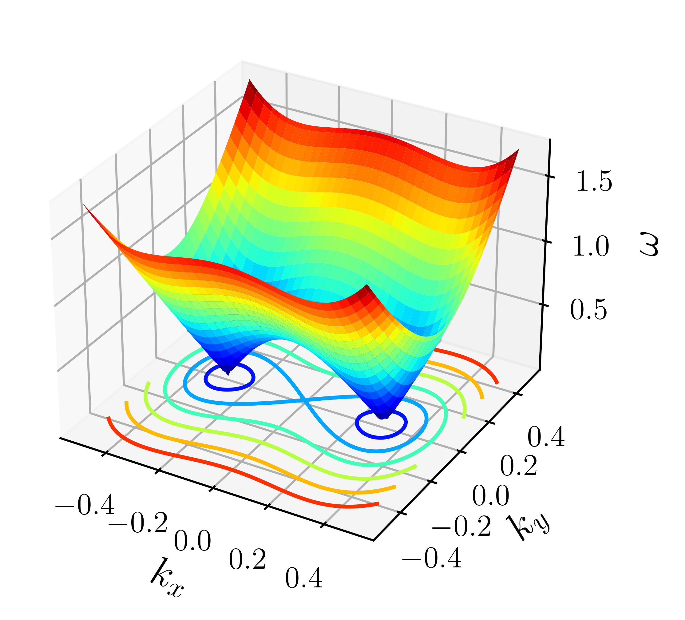
Figure 4: Dirac cones. We plot the positive root of Eq. (35) for parameters: $T_{x}=T_{y}=3$ and $T_{0}=-2.5$ with two Dirac points.

IV.2 The Lieb lattice

In this section, we consider the synthesis of a Lieb lattice dispersion relation [5, 6, 7], using a form of Eq. (31) which results in an effective spin $S=1$ with a flat band. The idea is sketched in Fig. 5: it essentially consists in creating different types of sites: $A,$ $B$, coupled with coupling $T_{x}$, $B$ and $C$ coupled with $T_{y}$, while sites $D$ are completely uncoupled and thus dynamically irrelevant.

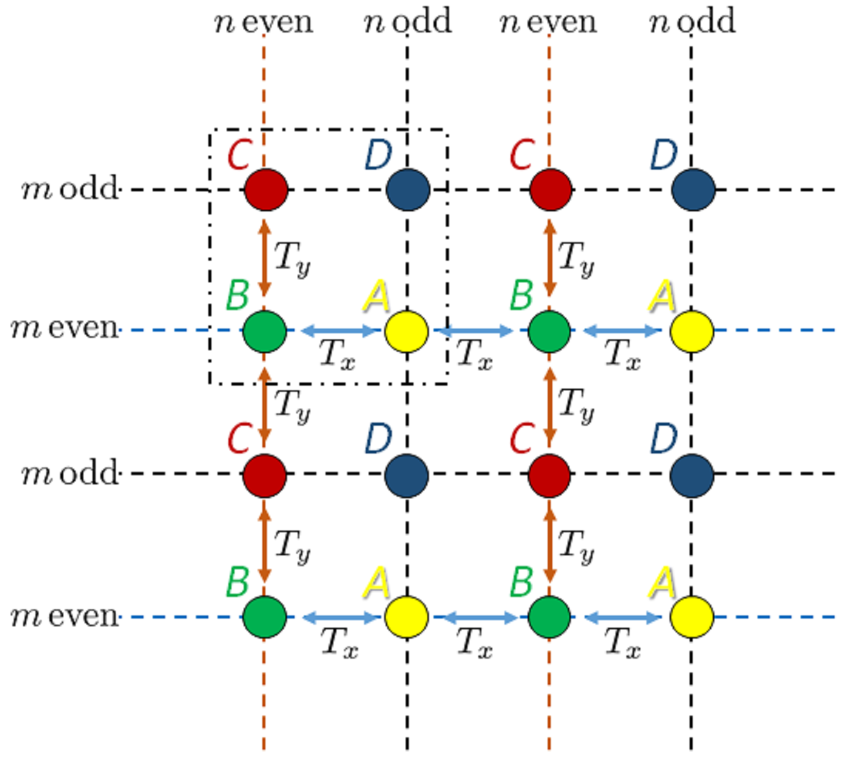
Figure 5: Synthesis of a Lieb lattice. The unit cell is indicated by the dashed-dotted square. Sites $D$ ($n$ and $m$ odd) are uncoupled to their neighbors. The other sites $A,$$B$ and $C$ are resonantly coupled to their neighbors: $B$ to $C$ with amplitude $T_{y}$ along the lines of $m$ even; $A$ to $B$ with amplitude $T_{x}$ along the lines of $n$ even.

This selective coupling can be obtained with the following perturbation

$$H_{1_{2D}}(x,y,t)=\cos\left(2\pi x\right) \left[V_{x}^{(1)}+V_{x}^{(2)}\cos(\pi y)\right]\cos\left(\omega_{B}^{(x)}t\right)+\cos\left(2\pi y\right)\left[V_{y}^{(1)}+V_{y}^{(2)}\cos(\pi x)\right]\cos\left(\omega_{B}^{(y)}t\right).$$

Substituting the general solution of Eq. (32) in Schrödinger’s equation for the Hamiltonian $H_{0_{2D}}+H_{1_{2D}}$ one obtains the following set of coupled equation (in the resonant approximation)

$$\mathrm{i}\frac{dc_{n,m}}{dt}= T_{x}\left[1+(-1)^{m}\right]\left(c_{n+1,m}+c_{n-1,m}\right)$$

$$+T_{y}\left[1+(-1)^{n}\right]\left(c_{n,m+1}+c_{n,m-1}\right)$$ (36)

with couplings

$$T_{x} =\frac{1}{2}V_{x}^{(1)}\left\langle\varphi_{0}^{(x)}\right|\cos\left(2\pi x\right)\left|\varphi_{1}^{(x)}\right\rangle$$

$$T_{y} =\frac{1}{2}V_{y}^{(1)}\left\langle\varphi_{0}^{(y)}\right|\cos\left(2\pi y\right)\left|\varphi_{1}^{(y)}\right\rangle$$

provided that the modulation amplitudes obey the following relations

$$V_{x}^{(1)} = V_{x}^{(2)}\left\langle\varphi_{0}^{(y)}\right|\cos\left(\pi y\right)\left|\varphi^{(y)}\right\rangle$$

$$V_{y}^{(1)} = V_{y}^{(2)}\left\langle\varphi_{0}^{(x)}\right|\cos\left(\pi x\right)\left|\varphi^{(x)}\right\rangle.$$

As expected, Eqs. (36) show that the complex amplitudes $c_{n,m}$ with $n$ and $m$ odd (corresponding to $D$ sites) are dynamically inert. These amplitudes are therefore irrelevant and, as shown in Fig. 5, the effective unit cell contains only three relevant sites, which is the characteristic of Lieb lattices.

In the same spirit as in Sec. IV.1 we define three amplitudes in $k$-space

$$\tilde{c}(k_{x},k_{y},t)=\sum_{n\textrm{ even }}\sum_{m\textrm{ even }}c_{nm}(t)\mathrm{e}^{-\mathrm{i}nk_{x}}\mathrm{e}^{-\mathrm{i}mk_{y}},$$

and $\tilde{d}(k_{x},k_{y},t)$ for $m$ even, $n$ odd, and $\tilde{f}(k_{x},k_{y},t)$ for $m$ odd, $n$ even. The time-evolution in $k$-space for the three-component spinor $\left[\psi\right]=\left(\tilde{c}(k_{x},k_{y},t),\tilde{d}(k_{x},k_{y},t),\tilde{f}(k_{x},k_{y},t)\right){}^{\mathsf{T}}$ obeys

$$\mathrm{i}\frac{d\left[\psi\right]}{dt}=\left[\begin{array}[]{ccc}0&4T_{y}\cos k_{y}&4T_{x}\cos k_{x}\\ 4T_{y}\cos k_{y}&0&0\\ 4T_{x}\cos k_{x}&0&0\end{array}\right]\left[\psi\right]$$

leading to the well-known three-band dispersion relations of the Lieb lattice:

$$\omega(k_{x},k_{y}) = 0$$

$$\omega(k_{x},k_{y}) = \pm\sqrt{\left(4T_{x}\cos k_{x}\right)^{2}+\left(4T_{y}\cos k_{y}\right)^{2}}$$ (37)

where the first relation corresponds to the flat band and the second one to two symmetric bands, and is anisotropic if $T_{x}\neq T_{y}$, as shown in Fig. 6.

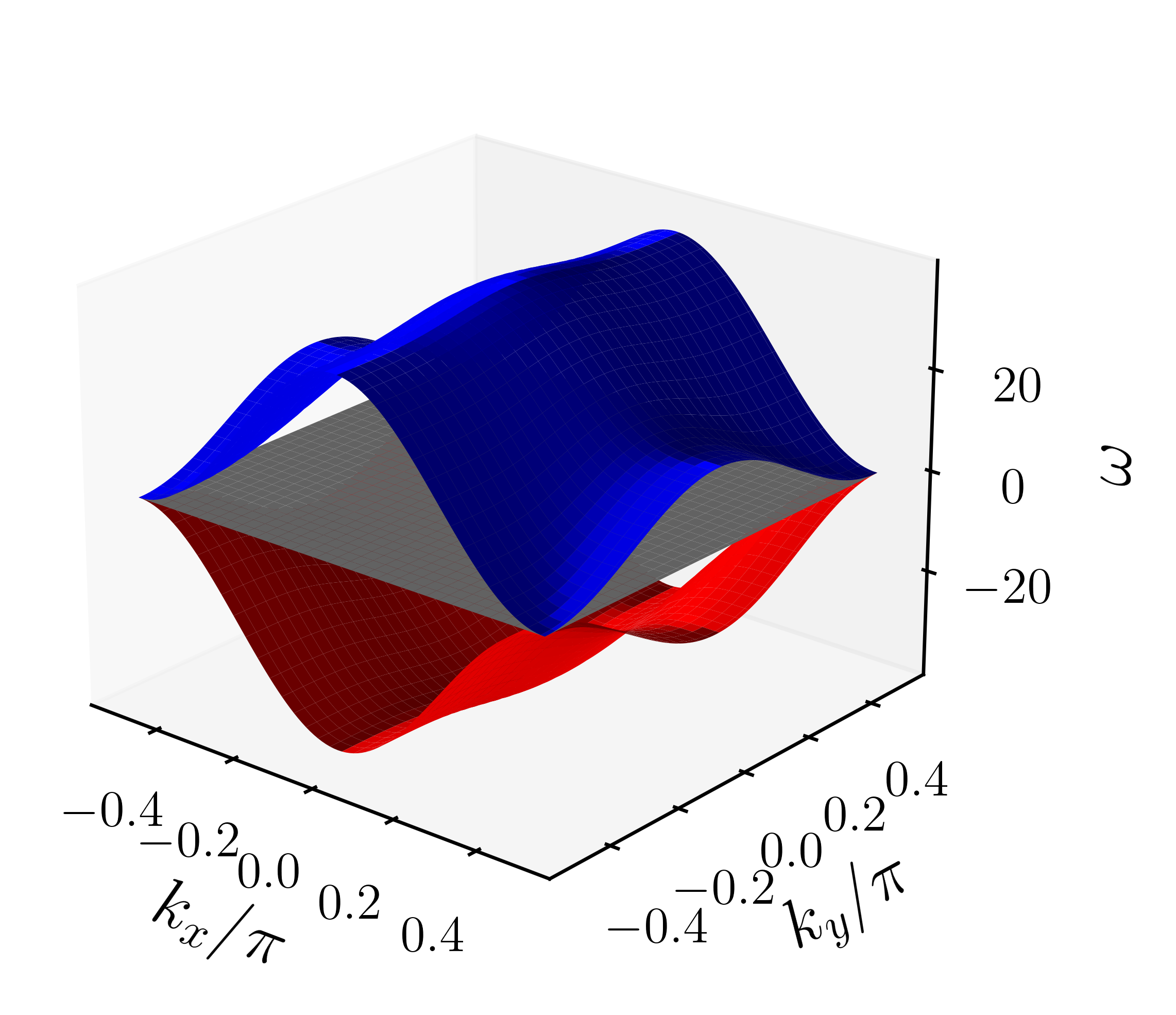
Figure 6: Lieb lattice dispersion relation, Eq. (37). Parameters are $T_{x}=1.5$, $T_{y}=1$.

V Conclusion

We introduced in this work a technique allowing the generation of arbitrary dispersion relations in a tilted modulated lattice, which we illustrated through several important examples: the 1D Dirac phononic dispersion relation, the Bogoliubov dispersion relation, the Landau superfluid relation, with the maxon and the roton features. We proposed a simple way to experimentally detect the dispersion relation by adding a slow chirp to the modulation and measuring an easily accessible quantity, namely the average position of the wave packet. Finally, we illustrated a generation of Dirac points in 2 dimensions and the generation of a flat band in a Lieb lattice. The technique introduced in the present work thus appears as an efficient, state-of-the-art experimentally feasible, way to synthesize lattice systems with arbitrary dispersion relations, thus mimic a large variety of important condensed matter systems.

Appendix A Dynamics in a chirped lattice

In this appendix we show how the introduction of a chirp allows to extract the shape of the dispersion relation from the measurement of the average wave packet position evolution.

Consider a smooth wave packet in a system obeying a dispersion relation $\omega(k,t)$. Its average position $\left\langle X\right\rangle(t)$ can be written as

$$\left\langle X\right\rangle(t)=\left\langle X\right\rangle(t=0)+\int_{0}^{t}v_{G}(t^{\prime})dt^{\prime}$$

where $v_{G}(t)=d\omega/dk$ is the group velocity.

An adiabatic chirp $\varphi(t)=\gamma t$ corresponds to $k(t)=k_{0}+\gamma t$, and thus, by integration

$$\left\langle X\right\rangle(t)=\left\langle X\right\rangle(t=0)+\left[\omega\left(k(t)\right)-\omega\left(k_{0}\right)\right]/\gamma$$

with $\left\langle X\right\rangle(t=0)=0$. Choosing $k_{0}$ such that $\omega(k_{0})=0$ this results in the simple expression:

$$\left\langle X\right\rangle(t)=\omega\left(k(t)\right)/\gamma.$$

Hence, measuring of the temporal evolution of the average position of the wave packet directly gives the shape of dispersion relation.

References

- Landau [1941] L. Landau, Theory of the Superfluidity of Helium II, Phys. Rev. 60, 356 (1941).
- Leggett [2006] A. Leggett, Quantum Liquids: Bose condensation and Cooper pairing in condensed-matter systems (Oxford Science Publications, Oxford, UK, 2006).
- Barenghi and Parker [2016] C. F. Barenghi and N. G. Parker, A primer on quantum fluids, arXiv:cond-mat.quant-gas/1605.09580 (2016).
- Jo et al. [2012] G.-B. Jo, J. Guzman, C. K. Thomas, P. Hosur, A. Vishwanath, and D. M. Stamper-Kurn, Ultracold Atoms in a Tunable Optical Kagome Lattice, Phys. Rev. Lett. 108, 045305 (2012).
- Slot et al. [2017] M. R. Slot, T. S. Gardenier, P. H. Jacobse, G. C. P. van Miert, S. N. Kempkes, S. J. M. Zevenhuizen, C. M. Smith, D. Vanmaekelbergh, and I. Swart, Experimental realization and characterization of an electronic Lieb lattice, Nat. Phys. 13, 672 (2017).
- Goldman et al. [2011] N. Goldman, D. F. Urban, and D. Bercioux, Topological phases for fermionic cold atoms on the Lieb lattice, Phys. Rev. A 83, 063601 (2011).
- Flannigan et al. [2021] S. Flannigan, L. Madail, R. G. Dias, and A. J. Daley, Hubbard models and state preparation in an optical Lieb lattice, arXiv:cond-mat.quant-gas/2101.03819 (2021).
- Roati et al. [2008] G. Roati, C. d’Errico, L. Fallani, M. Fattori, C. Fort, M. Zaccanti, G. Modugno, M. Modugno, and M. Inguscio, Anderson localization of a non-interacting Bose-Einstein condensate, Nature (London) 453, 895 (2008).
- Billy et al. [2008] J. Billy, V. Josse, Z. Zuo, A. Bernard, B. Hambrecht, P. Lugan, D. Clément, L. Sanchez-Palencia, P. Bouyer, and A. Aspect, Direct observation of Anderson localization of matter-waves in a controlled disorder, Nature (London) 453, 891 (2008).
- Moore et al. [1994] F. L. Moore, J. C. Robinson, C. Bharucha, P. E. Williams, and M. G. Raizen, Observation of Dynamical Localization in Atomic Momentum Transfer: A New Testing Ground for Quantum Chaos, Phys. Rev. Lett. 73, 2974 (1994).
- Ben Dahan et al. [1996] M. Ben Dahan, E. Peik, J. Reichel, Y. Castin, and C. Salomon, Bloch Oscillations of Atoms in an Optical Potential, Phys. Rev. Lett. 76, 4508 (1996).
- Wilkinson et al. [1996] S. R. Wilkinson, C. F. Bharucha, K. W. Madison, Q. Niu, and M. G. Raizen, Observation of Atomic Wannier-Stark Ladders in an Accelerating Optical Potential, Phys. Rev. Lett. 76, 4512 (1996).
- Jaksch et al. [1998] D. Jaksch, C. Bruder, J. I. Cirac, C. W. Gardiner, and P. Zoller, Cold Bosonic Atoms in Optical Lattices, Phys. Rev. Lett. 81, 3108 (1998).
- Greiner et al. [2002] M. Greiner, O. Mandel, T. Esslinger, T. W. Hänsch, and I. Bloch, Quantum phase transition from a superfluid to a Mott insulator in a gas of ultracold atoms, Nature (London) 415, 39 (2002).
- Trimborn et al. [2009] F. Trimborn, D. Witthaut, and H. J. Korsch, Beyond mean-field dynamics of small Bose-Hubbard systems based on the number-conserving phase-space approach, Phys. Rev. A 79, 013608 (2009).
- Moore et al. [1995] F. L. Moore, J. C. Robinson, C. F. Bharucha, B. Sundaram, and M. G. Raizen, Atom Optics Realization of the Quantum Rotor, Phys. Rev. Lett. 75, 4598 (1995).
- Chabé et al. [2008] J. Chabé, G. Lemarié, B. Grémaud, D. Delande, P. Szriftgiser, and J. C. Garreau, Experimental Observation of the Anderson Metal-Insulator Transition with Atomic Matter Waves, Phys. Rev. Lett. 101, 255702 (2008).
- Gerritsma et al. [2010] R. Gerritsma, G. Kirchmair, F. Zahringer, E. Solano, R. Blatt, and C. F. Roos, Quantum simulation of the Dirac equation, Nature (London) 463, 68 (2010).
- Witthaut et al. [2011] D. Witthaut, T. Salger, S. Kling, C. Grossert, and M. Weitz, Effective Dirac dynamics of ultracold atoms in bichromatic optical lattices, Phys. Rev. A 84, 033601 (2011).
- Tarruell et al. [2012] L. Tarruell, D. Greif, T. Uehlinger, G. Jotzu, and T. Esslinger, Creating, moving and merging Dirac points with a Fermi gas in a tunable honeycomb lattice, Nature (London) 483, 302 (2012).
- Garreau and Zehnlé [2017] J. C. Garreau and V. Zehnlé, Simulating Dirac models with ultracold atoms in optical lattices, Phys. Rev. A 96, 043627 (2017).
- Garreau and Zehnlé [2020] J. C. Garreau and V. Zehnlé, Analog quantum simulation of the spinor-four Dirac equation with an artificial gauge field, Phys. Rev. A 101, 053608 (2020).
- Kondov et al. [2011] S. S. Kondov, W. R. McGehee, J. J. Zirbel, and B. DeMarco, Three-Dimensional Anderson Localization of Ultracold Matter, Science 334, 66 (2011).
- Jendrzejewski et al. [2012] F. Jendrzejewski, A. Bernard, K. Müller, P. Cheinet, V. Josse, M. Piraud, L. Pezzè, L. Sanchez-Palencia, A. Aspect, and P. Bouyer, Three-dimensional localization of ultracold atoms in an optical disordered potential, Nat. Phys. 8, 398 (2012).
- Semeghini et al. [2015] G. Semeghini, M. Landini, P. Castilho, S. Roy, G. Spagnolli, A. Trenkwalder, M. Fattori, M. Inguscio, and G. Modugno, Measurement of the mobility edge for 3D Anderson localization, Nat. Phys. 11, 554 (2015).
- Gerritsma et al. [2011] R. Gerritsma, B. P. Lanyon, G. Kirchmair, F. Zähringer, C. Hempel, J. Casanova, J. J. García-Ripoll, E. Solano, R. Blatt, and C. F. Roos, Quantum Simulation of the Klein Paradox with Trapped Ions, Phys. Rev. Lett. 106, 060503 (2011).
- Suchet et al. [2016] D. Suchet, M. Rabinovic, T. Reimann, N. Kretschmar, F. Sievers, C. Salomon, J. Lau, O. Goulko, C. Lobo, and F. Chevy, Analog simulation of Weyl particles with cold atoms, EPL (Europhysics Letters) 114, 26005 (2016).
- Cohen-Tannoudji and Guéry-Odelin [2011] C. Cohen-Tannoudji and D. Guéry-Odelin, Advances In Atomic Physics: An Overview (World Scientific Publishing, Singapore, 2011).
- Manai et al. [2015] I. Manai, J.-F. Clément, R. Chicireanu, C. Hainaut, J. C. Garreau, P. Szriftgiser, and D. Delande, Experimental Observation of Two-Dimensional Anderson Localization with the Atomic Kicked Rotor, Phys. Rev. Lett. 115, 240603 (2015).
- Note [1] The force can be generated by applying a linear chirp to one of the beams forming the standing wave, so that the nodes of the resulting standing wave are uniformly accelerated. In the (non-inertial) reference frame where the standing wave is at rest, the atoms feel a constant inertial force.
- Wannier [1937] G. H. Wannier, The Structure of Electronic Excitation Levels in Insulating Crystals, Phys. Rev. 52, 191 (1937).
- Glück et al. [1999] M. Glück, A. R. Kolovsky, and H. J. Korsch, Lifetime of Wannier-Stark states, Phys. Rev. Lett. 83, 891 (1999).
- Glück et al. [2000] M. Glück, M. Hankel, A. R. Kolovsky, and H. J. Korsch, Wannier-Stark ladders in driven optical lattices, Phys. Rev. A 61, 061402(R) (2000).
- Haroutyunyan and Nienhuis [2001] H. L. Haroutyunyan and G. Nienhuis, Coherent control of atom dynamics in an optical lattice, Phys. Rev. A 64, 033424 (2001).
- Thommen et al. [2002] Q. Thommen, J. C. Garreau, and V. Zehnlé, Theoretical analysis of quantum dynamics in one-dimensional lattices: Wannier-Stark description, Phys. Rev. A 65, 053406 (2002).
- Glück et al. [2002] M. Glück, A. R. Kolovsky, and H. J. Korsch, Wannier-Stark resonances in optical and semiconductor superlattices, Phys. Rep. 366, 103 (2002).
- Plötz et al. [2021] P. Plötz, P. Schlagheck, and S. Wimberger, Effective spin model for interband transport in a Wannier-Stark lattice system, Eur. Phys. J. D 63, 47 (2021).
- Note [2] The translation symmetry implies for .
- Pethick and Smith [2008] C. J. Pethick and H. Smith, Bose-Einstein Condensation in Dilute Gases, 2nd ed. (Cambridge University Press, Cambridge, UK, 2008).
- Note [3] The roton minimum determines Landau’s critical velocity given by slope of the dispersion relation, thus setting a gap responsible for the superfluidity.
- Ha et al. [2015] L.-C. Ha, L. W. Clark, C. V. Parker, B. M. Anderson, and C. Chin, Roton-Maxon Excitation Spectrum of Bose Condensates in a Shaken Optical Lattice, Phys. Rev. Lett. 114, 055301 (2015).
- Chomaz et al. [2018] L. Chomaz, R. M. W. van Bijnen, D. Petter, G. Faraoni, S. Baier, J. H. Becher, M. J. Mark, F. Wächtler, L. Santos, and F. Ferlaino, Observation of roton mode population in a dipolar quantum gas, Nat. Phys. 14, 442 (2018).
- Santos et al. [2003] L. Santos, G. V. Shlyapnikov, and M. Lewenstein, Roton-Maxon Spectrum and Stability of Trapped Dipolar Bose-Einstein Condensates, Phys. Rev. Lett. 90, 250403 (2003).
- Chen et al. [2021] Y. Chen, M. Kadic, and M. Wegener, Roton-like acoustical dispersion relations in 3D metamaterials, Nat. Commun. 12, 3278 (2021).
- Note [4] That is, acts as a (time-dependent) quasimomentum.
- Montambaux et al. [2009] G. Montambaux, F. Piéchon, J.-N. Fuchs, and M. O. Goerbig, Merging of Dirac points in a two-dimensional crystal, Phys. Rev. B 80, 153412 (2009).