Dense Supervision Propagation for Weakly Supervised Semantic Segmentation on 3D Point Clouds

Abstract

Semantic segmentation on 3D point clouds is an important task for 3D scene understanding. While dense labeling on 3D data is expensive and time-consuming, only a few works address weakly supervised semantic point cloud segmentation methods to relieve the labeling cost by learning from simpler and cheaper labels. Meanwhile, there are still huge performance gaps between existing weakly supervised methods and state-of-the-art fully supervised methods. In this paper, we train a semantic point cloud segmentation network with only a small portion of points being labeled. We argue that we can better utilize the limited supervision information as we densely propagate the supervision signal from the labeled points to other points within and across the input samples. Specifically, we propose a cross-sample feature reallocating module to transfer similar features and therefore re-route the gradients across two samples with common classes and an intra-sample feature redistribution module to propagate supervision signals on unlabeled points across and within point cloud samples. We conduct extensive experiments on public datasets S3DIS and ScanNet. Our weakly supervised method with only 10% and 1% of labels can produce compatible results with the fully supervised counterpart.

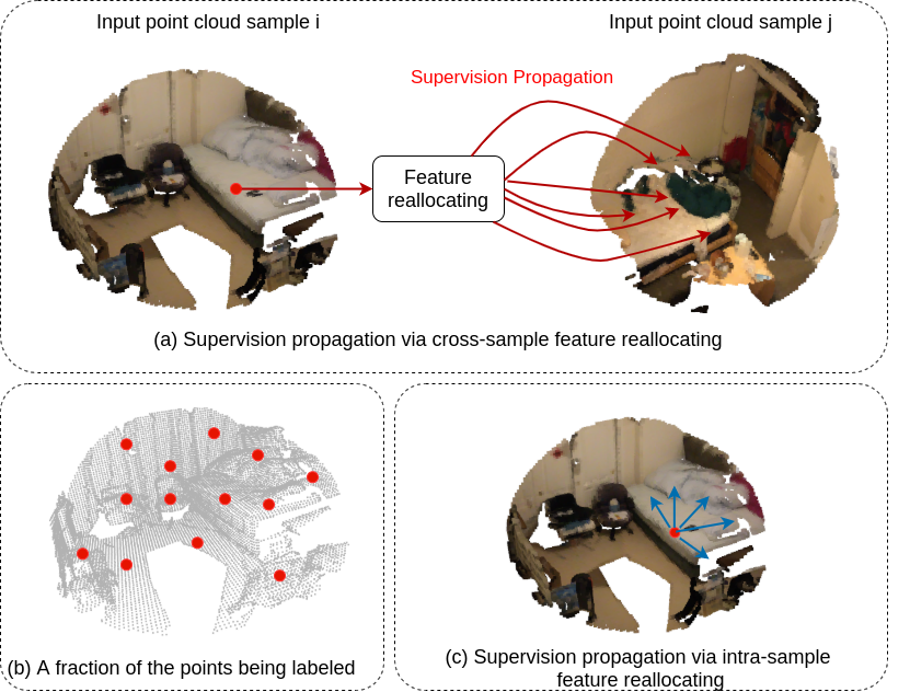
Figure 1: (a) Supervision propagation across samples via cross-sample feature reallocating. For clarity, this figure shows only single direction of the feature reallocating and supervision propagation, the module can propagate supervision bidirectionally. (b) An illustration of our weak labels. (c) Supervision propagation within samples via intra-sample feature reallocating.

1 Introduction

Semantic point cloud segmentation is vital for 3D scene understanding, which provides fundamental information for further applications like augmented reality and mobile robots. Recent developments in deep learning based point clouds analysis methods have made considerable progress in 3D semantic segmentation[11, 6, 10, 25]. However, 3D semantic segmentation requires point-level labels, which are much more expensive and time-consuming than the labels of 3D classification and detection tasks.

Recently, many efforts are put into weakly supervised semantic segmentation (WSSS) on 2D images and achieves remarkable results. However, despite dense labeling on point clouds is even more expensive than dense image labeling, only a few works have been done on 3D WSSS and yet remains a huge performance gap with the state-of-the-art fully supervised methods.

The existing 3D WSSS methods form the problem in different directions. [27] utilize dense 2D segmentation labels to supervise the training in 3D by projecting the 3D predictions onto the corresponding 2D labels. However, each 3D sample is projected to 2D in several views and each projected 2D image needs pixel-level labeling. Thus, this method still requires a large amount of manual labeling. [31] proposes to generate pseudo point-level label using 3D class activation map[36] from subcloud-level annotation, which is similar to the 2D WSSS methods using image-level labels. [34] directly trains a point cloud segmentation network with 10 time fewer labels, which is close to point supervision[3] and scribble supervision[18, 26] in 2D WSSS methods. We adopt the 3D WSSS setting from [34] that taking only a small fraction of points to be labeled.

In this work, we aim to better utilize the limited annotations by densely propagate the supervision signals from labeled points to unlabeled points. Concretely, we first adopt the state-of-the-art point cloud segmentation network KPConv[25] as our basic model. The basic model can be regarded as a normal point cloud segmentation network trained with partial labels. To address the problems stated above, we propose a two stage training strategy with our cross-sample feature reallocating module (CSFR) and intra-sample feature reallocating (ISFR) module respectively.

In the first training stage, inspired by [23, 19, 9], we choose two samples with at least one common classes as an input pair. A cross-sample feature reallocating module is trained to transfer similar features across two samples. However, different from [23, 19, 9] which directly add the warped features from another sample to find more activated region, we reconstruct the features from another sample using the point correlation between the data pair instead of adding them to the current feature. The each point in reconstructed feature can be considered as a weighted sum of all points from the other sample. Then, we use a cross regularization loss to softly pose the weak supervision on the reallocated features. Therefore, we can re-route the gradients to densely propagate supervision from the labeled points in one sample to the unlabeled points in the other sample. In the second training stage, we propagate the supervision from labeled points to unlabeled points within each sample with our intra-sample feature reallocating module. Similarly, we reallocate the features based on point correlation. Therefore, we can densely propagate the supervision from the labeled points to unlabeled points within the sample. Since there may exist uncommon classes between input pairs, which could bring some noisy during supervision propagation, we train the network with CSFR module to learn general representations first and train the network with ISFR module as finetuning in the second stage. Since the two modules are based on point correlations, supervision signals can be propagate to the unlabeled points with similar features of the labeled points. Noted that these two modules are only used to help the training of the basic network. We do not need these modules to generate the final segmentation predictions during inference. The two modules implicitly guide the training of the basic segmentation network, and will be discarded at test time.

In summary, our contributions are:

• We propose a cross-sample feature reallocating module to reconstruct features and re-route gradients across the input pair based on point correlation. Hence, the supervision signals from labeled points can be propagated to unlabeled points across samples.

• We propose an intra-sample feature reallocating module to reallocate features within each sample based on point correlation. Then, the supervision signals can be propagated from labeled points to unlabeled points within each point cloud sample.

• We propose a two stage training strategy so the cross-sample feature reallocating module and the intra-sample feature reallocating module can both contribute to the performance without interfering each other.

• Our weakly supervised methods with only 10% and 1% of the points being labeled can produce compatible results with their fully supervised counterpart in S3DIS and ScanNet dataset.

2 Related Works

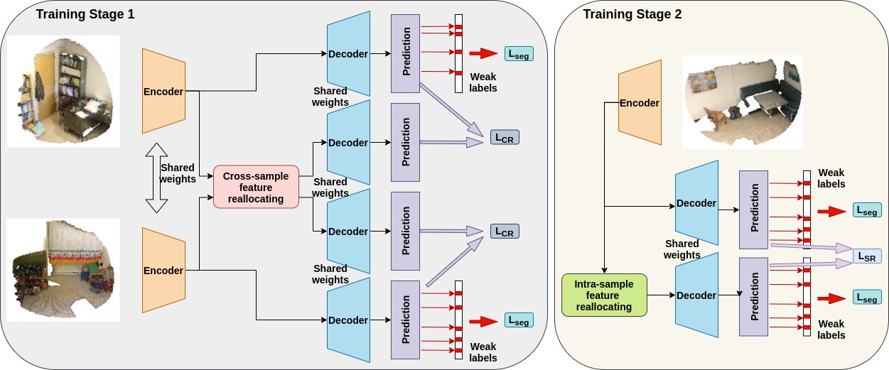
Figure 2: The overall two stage training framework for our proposed method. Left: The first training stage. Two point cloud samples are fed into the network as an input pair. A cross-sample feature reallocating module is designed to reallocate features and re-route gradients to propagate supervision signals across the input pairs. Right: The second training stage. Each point cloud sample is fed into the network independently. An intra-sample feature propagation module is designed to propagate supervision signals within the samples. Noted that the encoder and decoder blocks are the same during the two training stages, the parameters of encoder and decoder are passed to stage 2 after training in stage 1. All the encoders and all the decoders share the same parameters within each training stage.

2.1 Semantic Segmentation on 3D Point clouds

There are mainly three categories for 3D semantic segmentation methods: projection-based methods, voxel-based methods and point-based methods. Multi-view projection based methods[16, 35, 8] project the 3D data into 2D from multiple viewpoints, therefore they can easily process the projected data on 2D convolution networks. However, these methods suffer from occlusion, view-point selection, misalignment and other defects that may limit the performance. Voxel-besed methods like Submanifold Sparse Convolution[10], MinkowskiNet[6] and Occuseg[11] first quantize the point cloud data into voxels and perform sparse 3D convolution on the voxels. These methods can often achieve good segmentation performance but severely suffer from heavy memory and time consumption. Point based methods directly take raw point cloud data as network input. PointNet[20] and PointNet++[21] process point cloud data with stacked MLPs. DGCNN[29] proposes EdgeConv to capture local geometry by dynamically generating graphs for points with their neighbors. PointCNN[17] and PointConv[33] formulate convolution operations in 3D using KNNs for each point. KPConv[25] uses filters and kernel points in euclidean space to formulate convolution operation with distances of points within the filter.

2.2 Weakly supervised 2D semantic segmentation

Most 2D WSSS methods are using image-level labels. Based on class activation map(CAM)[36], many methods[30, 32, 14, 22, 22, 1, 15, 23, 19, 9] refines the CAM generated from a classification network to generate pseudo pixel-level labels. Then, segmentation networks are trained using the pseudo pixel-level labels. Besides image-level label, there other kinds of weak labels like point supervision[3] and scribble supervision[18, 26] which is similar to the weak setting in this work. Points and scribble supervision methods usually constrain the unlabeled points using label consistency with local smoothness.

2.3 Weakly supervised 3D semantic segmentation

Existing 3D WSSS methods utilize different kinds of weak supervisions.[27] utilize dense 2D segmentation labels to supervise the training in 3D by projecting the 3D predictions onto the corresponding 2D labels. [31] proposes to generate pseudo point-level label using 3D class activation map[36] from subcloud-level annotation. [34] directly trains a point cloud segmentation network with 10 time fewer labels.

3 Approach

As illustrated in Fig.2, we propose a two stage training strategy. In the first training stage, we train the basic segmentation network with the cross-sample feature reallocating module. And in the second stage, we train the the basic segmentation network with the intra-sample feature reallocating module. We will explain each module in detail.

3.1 Basic segmentation network

The basic component of our method is a point cloud segmentation network. We take the state-of-the-art deep learning architecture Kernel Point Convolution(KPConv)[25] segmentation network as our backbone network. We denote each input point cloud sample as $\bm{P}_{i}\in\mathbb{R}^{N_{i}\times D}$ where $N_{i}$ is the input point number and $D$ is the input feature dimension. After feeding the $\mathit{P_{i}}$ to the encoder, we get the encoded feature map $\bm{F}_{i}=f_{enc}(\bm{P}_{i})\in\mathbb{R}^{N^{e}_{i}\times K}$, where $N^{e}_{i}$ is the down-sampled point numbers for sample $i$ and $K$ is the feature dimension. The encoded feature $\bm{F}_{i}$ is then fed into the decoder to get the final prediction $\bm{Z}_{i}=f_{dec}(\bm{F}_{i})\in\mathbb{R}^{N\times C}$, where $C$ is the number of classes. The one-hot label of the sample is denoted as $\bm{Y}_{i}\in\mathbb{R}^{N\times C}$. However, as we only have labels for a small fraction of the points, we define a binary mask $\bm{M}\in\mathbb{R}^{N}$ to indicate whether a point is being labeled, the mask is 1 for labeled points and 0 for unlabeled points. Then, a weakly supervised softmax cross-entropy loss is calculated on the labeled points as:

$$\mathcal{L}_{seg\_basic}=-\frac{1}{\bm{B}}\displaystyle\sum_{n}\bm{m}_{n}\displaystyle\sum_{c}\bm{y}_{nc}\frac{e^{\bm{z}_{nc}}}{\displaystyle\sum_{c}e^{\bm{z}_{nc}}}$$ (1)

where $\bm{B}=\displaystyle\sum_{n}\bm{m}_{n}$ is a normalization factor.

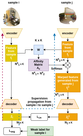
Figure 3: This blue dotted line illustrates how the weak supervision from sample $i$ is propagated to sample $j$ based on point correlation. For clarity, this figure shows only single direction of the feature reallocating and supervision propagation, the module can propagate supervision bidirectionally.

3.2 Cross-sample feature reallocating

We take two point cloud samples $\bm{P}_{i}\in\mathbb{R}^{N_{i}\times D}$ and $\bm{P}_{j}\in\mathbb{R}^{N_{j}\times D}$ with at least one common label as an input pair. We feed the input pair into the KPConv encoder in the basic network and get the feature maps $\bm{F}_{i}\in\mathbb{R}^{N^{e}_{i}\times K}$ and $\bm{F}_{j}\in\mathbb{R}^{N^{e}_{j}\times K}$.

The feature reallocating is achieved by warping point features using the point correlation between the input samples. We first calculate a cross affinity matrix $\bm{A}_{c}$ between the two features. With a learnable matrix $\bm{W}_{c}\in\mathbb{R}^{K\times K}$, the affinity matrix is derived as:

$$\bm{A}_{c}=\bm{F}_{i}\bm{W}_{c}\bm{F}^{\top}_{j}\in\mathbb{R}^{N^{e}_{i}\times N^{e}_{j}}$$ (2)

The cross affinity matrix describes the point-wise similarity between all pair of points in two samples. We then normalize the cross affinity matrix row-wise and column-wise to guide the feature reallocating for each point:

$$\begin{split}&\bm{A}^{i}_{c}=softmax(\bm{A}_{c})\\ &\bm{A}^{j}_{c}=softmax(\bm{A}^{\top}_{c})\end{split}$$ (3)

Then, we use the normalized affinity to guide the feature reallocating:

$$\begin{split}&\bm{F}^{c}_{j}=\bm{F_{j}}\bm{A}^{j}_{c}\in\mathbb{R}^{N^{e}_{i}\times K}\\ &\bm{F}^{c}_{i}=\bm{F_{i}}\bm{A}^{i}_{c}\in\mathbb{R}^{N^{e}_{j}\times K}\end{split}$$ (4)

The warped feature maps $\bm{F}^{c}_{j}$ and $\bm{F}^{c}_{i}$ have the same size and spatial shape with the original feature maps $\bm{F}_{i}$ and $\bm{F}_{j}$. However, all the features in $\bm{F}^{c}_{j}$ are collected from sample $\bm{P}_{j}$ and each point feature in $\bm{F}^{c}_{j}$ can be seen as a weighted sum of all point features from $\bm{F}_{j}$, which means we constructed a new feature $\bm{F}^{c}_{j}$ in the shape of $\bm{F}_{i}$ using the features from $\bm{F}_{j}$ and vice versa.

Unlike the previous methods[23, 19, 9] which utilize common semantics from other samples and directly discover more object regions by generating pseudo labels. We feed the reallocated and original feature maps into the decoders with shared weights respectively. For sample $\bm{P}_{i}$ side, we feed the original feature map $\bm{F}_{i}$ and the reallocated feature map $\bm{F}^{c}_{j}$ from sample $\bm{P}_{j}$ into the decoder network and get the outputs $\bm{Z}_{i}=f_{dec}(\bm{F}_{i})\in\mathbb{R}^{N_{i}\times C}$ and $\bm{Z}^{c}_{j}=f_{dec}(\bm{F}^{c}_{j})\in\mathbb{R}^{N_{i}\times C}$.

Here we have the weak labels for sample $\bm{P}_{i}$ and each point in $\bm{F}^{c}_{j}$ can be seen as a weighted sum of all the points from sample $\bm{P}_{j}$. Therefore it is possible to densely propagate the supervision from the labeled points in sample $\bm{P}_{i}$ to the unlabeled points in sample $\bm{P}_{j}$ as we re-routed the gradients using the feature reallocating module. However, there may exist uncommon classes between the input samples, directly apply a weakly segmentation loss on the reallocated branch output may introduce noise into the training process. Thus, we do not calculate segmentation loss for the reallocated branch. Instead, inspired by [24, 4, 5], we first calculate a weak segmentation loss as in Equation 1 on the output of the original feature $\bm{Z}_{i}$ and propose a cross regularization(CR) loss to maximize the agreement between $\bm{Z}_{i}$ and $\bm{Z}^{c}_{j}$:

$$\mathcal{L}_{CR}=\|\bm{Z}_{i}-\bm{Z}^{c}_{j}\|^{2}_{F}=\|f_{dec}(\bm{F}_{i})-f_{dec}(\bm{F}^{c}_{j})\|^{2}_{F}$$ (5)

Therefore, we can softly propagate the supervision signal from the labeled in sample $\bm{P}_{i}$ to the unlabeled points in sample $\bm{P}_{j}$ and vice versa. In this way, each labeled points can transfer the supervision signals to those points with similar features in the other sample.

3.3 Intra-sample feature reallocating

In this section, we propose an intra-sample feature propagation(ISFR) module to further propagate supervision from labeled points to unlabeled points within each sample and finetuning the network against the possible noisy introduced from CSFR module. For each input sample $\bm{P}_{i}\in\mathbb{R}^{N_{i}\times D}$, we can get the feature map $\bm{F}_{i}\in\mathbb{R}^{N^{e}_{i}\times K}$ from the same encoder network. Similar to the previous module, we can calculate a self affinity matrix $\bm{A}_{s}$ for the feature:

$$\bm{A}_{s}=\bm{F}_{i}\bm{W}_{s}\bm{F}^{\top}_{i}\in\mathbb{R}^{N^{e}_{i}\times N^{e}_{i}}$$ (6)

where $\bm{W}_{s}\in\mathbb{R}^{K\times K}$ is a learnable matrix. The self affinity matrix describes the point-wise correlation between all points within the input sample. We then normalize the self affinity matrix to guide the feature reallocating for each point:

$$\bm{A}^{i}_{s}=softmax(\bm{A}^{\top}_{s})$$ (7)

Then, we use the normalized affinity to guide the feature warping:

$$\bm{F}^{s}_{i}=\bm{F_{i}}\bm{A}^{i}_{s}\in\mathbb{R}^{N^{e}_{i}\times K}\\$$ (8)

Unlike the classical self-attention[28], we remove the residual connection to retain the same activation intensity. Here each point in $\bm{F}^{s}_{i}$ can be considered as a weighted sum of all the points in the sample and the features are reallocated with respect to the point correlation. We separately feed the reallocated feature and the original feature to the decoder. Thus, the decoder outputs from the two branches are $\bm{Z}^{s}_{i}=f_{dec}(\bm{F}^{s}_{i})\in\mathbb{R}^{N_{i}\times C}$ and $\bm{Z}_{i}=f_{dec}(\bm{F}_{i})\in\mathbb{R}^{N_{i}\times C}$.

Similar to the cross regularization loss, we use a similar self regularization(SR) loss on the two outputs to regularize the reallocated feature with the original output:

$$\mathcal{L}_{SR}=\|\bm{Z}^{s}_{i}-\bm{Z}_{i}\|^{2}_{F}=\|f_{dec}(\bm{F}^{s}_{i})-f_{dec}(\bm{F}_{i})\|^{2}_{F}.$$ (9)

Since the features are reallocated within the samples and will not introduce supervision from absent classes like CSFR, we apply another weak segmentation loss to the self reallocating branch:

$$\mathcal{L}_{seg\_s}=-\frac{1}{\bm{B}}\displaystyle\sum_{n}\bm{m}_{n}\displaystyle\sum_{c}\bm{y}_{nc}\frac{e^{\bm{z}^{s}_{nc}}}{\displaystyle\sum_{c}e^{\bm{z}^{s}_{nc}}}.$$ (10)

where $\bm{B}=\displaystyle\sum_{n}\bm{m}_{n}$ is a normalization factor. Therefore, the supervision signals on the labeled points can be transferred to the unlabeled points with similar features.

3.4 Training

As shown in Fig.2, we use a two stage training strategy to avoid interference between the two modules during training. In stage one, we train the basic segmentation network with the cross-sample feature reallocating module. In this stage, for each sample, the network learns from the weak labels of this sample and the supervision propagated from the weak labels of another sample. The overall learning objective in stage one can be expressed as:

$$\mathcal{L}_{stage1}=\mathcal{L}_{seg\_basic}+\mathcal{L}_{CR}$$ (11)

In the second stage, we train the basic segmentation network with the intra-sample feature reallocating module. The second stage propagate supervision from labeled points to unlabeled points. The overall training objectives in stage two is:

$$\mathcal{L}_{stage2}=\mathcal{L}_{seg\_basic}+\mathcal{L}_{seg\_s}+\mathcal{L}_{SR}$$ (12)

We argue that joint training of the two modules would hamper the performance of the basic segmentation network since the cross regularization loss in CSFR module and the self regularization loss in ISFR module may interfere the training of each other as the CSFR module may bring wrong supervision from uncommon classes to the other sample, while the two stage training can avoid this issue and improve the performance by taking advantage of both the modules. We will further discuss this through experiments in section 4.3.

The two modules implicitly guide the optimization of basic network only at training time. In inference, we can simply discard the two modules and use the basic segmentation network as a normal point cloud segmentation network to get the segmentation predictions. Therefore, no extra memory and computational resources are introduced at test time.

modules	10% label	1% label
Baseline	66.5	65.1
One stage training
CSFR	67.7	66.8
ISFR	68.0	66.9
CSFR+ISFR	66.3	65.0
Two stage training
ISFR-CSFR	67.3	65.4
CSFR-ISFR	68.6	67.0

Table 1: Ablation study on one stage and two stage training. We evaluate each module in one stage training and the training orders in two stage training. Evaluated on S3DIS Area-5 in mIoU(%).

4 Experiments

4.1 Dataset

Dataset: We conduct our experiments on the popular public dataset S3DIS[2]. S3DIS covers 6 areas of entire floor from 3 different buildings with a total of 215 million points and covers over 6000$m^{2}$. The dataset is annotated with 13 classes. We follow the common practice that use Area 5 as test scene to measure the generalization ability. We also perform experiments on ScanNet[7] which contains 1513 scenes and annotated with 20 classes.

Weak labels: We follow [34] to annotate only 10% of the points. We first sample 4% of the points from the original data as the network inputs. Then, we randomly label 10% of points in each class for the sampled input point clouds. The final predictions will be back projected to the original point clouds. Therefore, only 10% of the network input training data and only 0.4% of the original point cloud data are labeled. We also perform experiments with fewer labels that only 1% of the input points are labeled.

4.2 Implementation details

We use the KPConv[25] segmentation model KPFCNN as our backbone network. The network is an encoder-decoder fully convolutional network with skip connections. The encoder is composed by bottleneck ResNet blocks[12] with KP convolution layers. The decoder part is composed by nearest upsampling layers with unary convolution layers. We put the CSFR and ISFR module after the first upsampling layer for larger spacial resolution. Due to the limitation in computational resources, we use ball query to sample point cloud as input samples, the sample radius is set to 2m. We use a Momentum SGD optimizer, the initial learning rate is set to 0.01 and the momentum is set to 0.98. We train the first stage for 600 epochs and the second stage for another 600 epochs.

CSFR
$\mathcal{L}_{seg\_basic}$	$\mathcal{L}_{CR}$	$\mathcal{L}_{seg\_c}$	10%	1%
✓			66.5	65.1
✓	✓		67.7	66.8
✓	✓	✓	66.3	64.8
(a)
ISFR
$\mathcal{L}_{seg\_basic}$	$\mathcal{L}_{SR}$	$\mathcal{L}_{seg\_s}$	10%	1%
✓			66.5	65.1
✓	✓		66.9	65.9
✓	✓	✓	68.0	66.9
(b)

Table 2: Ablation study on different losses within each module in mIoU(%). (a) illustrates the effectiveness of losses in CSFR module. We contact experiments with an additional $\mathcal{L}_{seg\_c}$ which is not included in the proposed method for comparison. (b) illustrates the effectiveness of losses in ISFR module.

setting	basic branch	cross branch	intra branch
ISFR-CSFR	67.3	60.3	66.6
CSFR-ISFR	68.6	62.2	67.4

Table 3: We compare the segmentation predictions in mIoU(%) from different decoder branches for the two stages trainings. Basic branch is the one we use for inference. Cross branch and intra branch are the decoder outputs produced from CSFR and ISFR propagated features.

4.3 Ablation studies

Two stage training versus joint training: Table 1 compares one stage training with two stage training performances trained with 10% and 1% labels. For one stage training, we perform experiments with only CSFR module or ISFR module, each of the module produces performance gain over the baseline method for both 10% and 1% label case. However, when we jointly train CSFR and ISFR modules in one stage, we observe a performance drop, producing results lower than solely training one module and even lower than the baseline method in both cases. From the experiments, we argue that the training losses in the two module may interfere each other during optimization. Since the CR loss and SR loss from the two modules both trying to pull the segmentation output closer to the outputs of the two branches, the overall training objective may be deviated from our real target, better segmentation performance. With the losses from two modules being optimised together, the model may fail to find the global optimum and being optimized toward wrong directions. Therefore, by separate the training into two stages, we can avoid the interference between the modules during training and take advantage of both the modules.

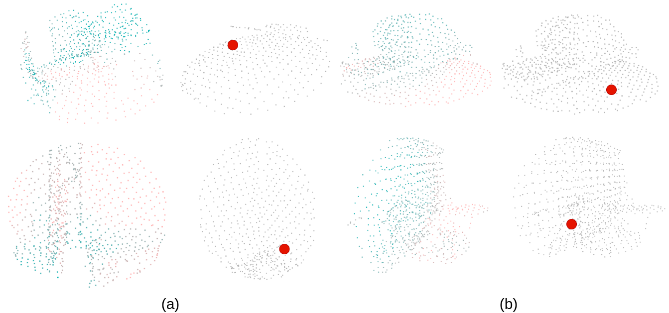
Figure 4: The visualization for the affinity calculated by (a)CSFR module, (b)ISFR module. The left side shows the corresponding affinity to the red point on the right part. Red means higher similarity and green means lower similarity.

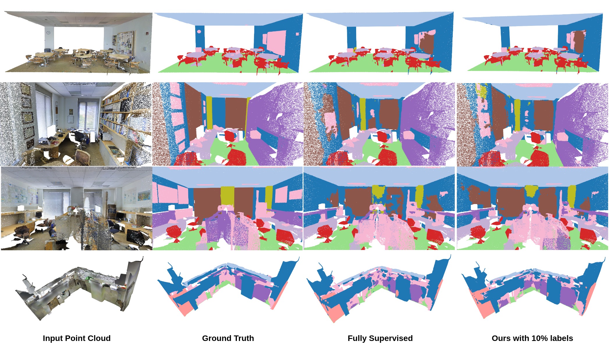
Figure 5: Visualizations on S3DIS Area-5. The results are, left to right, input RGB point cloud, ground truth, fully supervised method, our proposed method with 10% labels.

Training orders: We also compare the training orders of the two modules in Table 1. ISFR-CSFR means we train the network with ISFR module in the first stage and CSFR module in the second stage. CSFR-ISFR means that we train the network with CSFR module in the first stage and ISFR module in the second stage. We observe that CSFR-ISFR outperforms ISFR-CSFR under both 10% and 1% supervision. We argue that the CSFR module can help the network to learn more generalized coarse representations across samples while ISFR module can act like a finetuning module that finetune the learned representations to and impose constraints on unlabeled points within the samples. Therefore if we use the opposite training order, we can get worse results comparing to even each single modules.

Effects of different losses: We evaluate the effectiveness of each losses in Table 2 within in each module. We compare results with different combinations of the losses for a single stage training with only one module each. For the CSFR module, as shown in Table 2(a), we suppose $\mathcal{L}_{seg\_c}$ is a segmentation loss appended to the decoder of the cross propagated branch which we did not include in our architecture. We can observe that training with $\mathcal{L}_{seg\_basic}+\mathcal{L}_{CR}$ reaches best performance for the CSFR module for both the label settings which means the cross regularization loss helps the segmentation performance. We also observe that training with $\mathcal{L}_{seg\_basic}+\mathcal{L}_{CR}+\mathcal{L}_{seg\_c}$ produces even lower score than solely using $\mathcal{L}_{seg\_basic}$, which means adding another segmentation loss on the cross propagated decoder branch would harm the performance. This supports our statement in section 3.2 that additional supervision on the propagate branch would introduce noise into the training process since the inherent difference between two sample.

Table 2(b) shows that in the ISFR branch, training with all three losses $\mathcal{L}_{seg\_basic}+\mathcal{L}_{SR}+\mathcal{L}_{seg\_s}$ produces better results than using $\mathcal{L}_{seg\_basic}+\mathcal{L}_{SR}$ and solely using the segmentation loss on the original branch. This result supports our statement in section 3.3 that the ISFR module imposes constraints on unlabeled points within the sample. Since the feature propagation is processed inside each sample, no noises would be introduced to the training. Thus, calculating a segmentation loss on the propagated feature branch would improve the training results.

setting	model	mIoU	ceil.	floor	wall	beam	col.	wind.	door	chair	table	book.	sofa	board	clut.
Fully supervised
	PointNet[20]	41.1	88.8	97.3	69.8	0.1	3.9	46.3	10.8	52.6	58.9	40.4	5.9	26.4	33.2
	PointNet++[21]	47.8	90.3	95.6	69.3	0.1	13.8	26.7	44.1	64.3	70.0	27.8	47.8	30.8	38.1
	DGCNN[29]	47.0	92.4	97.6	74.5	0.5	13.3	48.0	23.7	65.4	67.0	10.7	44.0	34.2	40.0
	PointCNN[17]	57.3	92.3	98.2	79.4	0.0	17.6	22.8	62.1	80.6	74.4	66.7	31.7	62.1	56.7
	MinkNet[6]	65.4	91.8	98.7	86.2	0.0	34.1	48.9	62.4	89.8	81.6	74.9	47.2	74.4	58.6
	JSENet[13]	67.7	93.8	97.0	81.4	0.0	23.2	61.3	71.6	89.9	79.8	75.6	72.3	72.7	60.4
Paper	KPConv[25]	67.1	92.8	97.3	82.4	0.0	23.9	58.0	69.0	91.0	81.5	75.3	75.4	66.7	58.9
Retrain	KPConv[25]	67.3	94.8	98.4	82.3	0.0	28.3	56.6	71.2	90.5	82.6	74.6	67.8	67.4	59.9
Fully supervised	DSP(Ours)	68.5	94.3	98.4	83.7	0.0	28.9	59.1	73.4	91.2	82.2	75.3	73.9	68.5	61.0
Weakly supervised
2D dense label	GPFN[27]	50.8	-	-	-	-	-	-	-	-	-	-	-	-	-
10% label	WSPCS[34]	48.0	90.9	97.3	74.8	0.0	8.4	49.3	27.3	69.0	71.7	16.5	53.2	23.3	42.8
1% label	Baseline	65.1	93.8	97.9	81.8	0.0	28.6	57.1	67.6	89.1	79.7	73.4	59.7	65.9	59.9
1% label	DSP(Ours)	67.0	93.5	98.2	82.8	0.0	29.3	58.3	68.7	90.5	80.0	72.2	74.1	65.4	58.0
10% label	Baseline	66.5	94.5	98.4	82.9	0.0	26.8	56.3	71.8	90.6	82.0	75.4	59.7	65.9	59.9
10% label	DSP(Ours)	68.6	93.6	98.3	83.6	0.0	31.1	57.8	72.1	91.1	82.1	75.2	75.9	70.3	60.5

Table 4: The class-specific mIoU (%) evaluation on S3DIS Area-5. KPConv(paper) are taken from the paper reported score, KPConv(retrain) is the score from our basic segmentation network trained with 100% labels. The baseline methods means the basic segmentation network trained with only the weak labels and without CSFR and ISFR modules.

Performance of different branches: Table 3 compares the segmentation performance of different decoder branches in the two stage settings. In both settings, the cross branches produce poorest segmentation results the features of this branch are propagated from the other sample. However, the cross branch can still produce reasonable scores as the network is learned to only propagate features from same category for each point. The intra branch produces better results than the cross branch, but still lower than the basic branch. This supports our arguement that the ISFR module imposes more constraints to unlabeled points as the features of unlabeled points can be propagated to the labeled points in same category. But during inference, as the network already learned the representations, propagating the features is not helping the predictions. This is also a difference between our ISFR mudule with the self-attention module in many vision applications.

We also compare the results between the two settings. The outputs from all three branches in CSFR-ISFR performs better than those in ISFR-CSFR, which also supports our arguement in section 3.4. From the results, if ISFR module is trained first, the network can overfit within samples and not generalize across sample. Thus the cross branch performance is worse in ISFR-CSFR. Then, with the CSFR module trained in the second stage, the information from other samples may affect as noises. Therefore the performance from the basic branch is even lower than individually training with the two modules shown in Table 1.

4.4 Qualitative results

Fig.4(a) shows the affinity learned in CSFR between the input pairs. Fig.4(b) shows the affinity learned in ISFR in each sample. We show the affinity map on the left to the selected point on the right. The point clouds are sparse since we perform CSFR and ISFR in down-sampled features. Obviously, both the modules have successfully learned to propagate features from the same class.

We provide visualizations of our final segmentation predictions in Fig.5. We compare our results with the ground truth and the predictions from fully supervised counterpart. We can see that our method performs even better in label consistency and in hard examples like the fourth row.

4.5 Segmentation results

In Table 4, we compare our proposed method with state-of-the-art methods, other weakly supervised methods and our baseline method.

Comparison with baseline method: The baseline method is only the basic segmentation network trained with the weak labels. Ours method is the full model with cross- and intra-sample feature propagation modules and trained with the two stage strategy. The experiments show that our proposed method improves the performance of the baseline method with both 10% and 1% labels.

Comparison with existing 3D WSSS methods: We compare our proposed method with existing 3D WSSS methods[27, 34]. [27] utilizes 2D dense labels on 2D projections of the 3D point clouds and [34] utilize the same weak supervision technique by annotating 10% of the points. [34] can also produce close or better results to its fully supervised counterpart, but the overall performance still remain a huge gap with current state-of-the-art methods. Our proposed method surpass both of them by a large margin.

Comparison with fully supervised methods: We compare our weakly supervised method with some fully supervised state-of-the-art methods[20, 21, 29, 17, 6, 17, 25] on the public dataset S3DIS Area-5. Also, we compare our method under weak supervision against full supervision. Our method produce even slightly higher results using 10% label than trained under full supervision by 0.1%. We believe that supervision propagation is not that useful under full supervision as each point can directly get supervision information from its own label but it can still benefit from the self-attention like architecture. Therefore our 10% label results can produce similar results to the fully supervised counterpart.

Results on ScanNet: Table 5 shows the segmentation results in mIoU(%) in ScanNet[7] validation set. Our method outperforms the previous method MPRM[31] by a large margin. However, with 10% points labeled, the baseline results is already very close to the fully supervised results. We argue that ScanNet is a very large scale dataset, 10% of the label can already provide strong supervision. Our method is effective with only 1% labeled points, where we outperform the baseline method by 1.9% mIoU. In practice, it is not easy to collect a large scale dataset like ScanNet, we believe our method is meaningful in real-world applications.

Model	Supervision	mIoU
MPRM[31]	Sub-cloud label	43.2
KPConv-basic	Full supervision	71.2
KPConv-basic	1 % label	68.1
DSP (Ours)	1 % label	70.0
KPConv-basic	10 % label	71.1
DSP (Ours)	10 % label	71.6

Table 5: The segmentation results on ScanNet validation set. MPRM is another weakly supervised method using sub-cloud level supervision and developed also based on KPConv. The KPConv-basic means the basic network developed using KPConv.

5 Conclusion

In this paper, we propose a weakly supervised point cloud segmentation method with only 10% or 1% percent of the points being labeled. We developed cross- and intra-sample feature reallocating modules to densely propagate supervision from labeled points to unlabeled points. Our proposed method with 10% and 1% of the points being labeled can produce compatible results with its fully supervised counterpart in S3DIS and ScanNet dataset.

References

- [1] Jiwoon Ahn and Suha Kwak. Learning pixel-level semantic affinity with image-level supervision for weakly supervised semantic segmentation. In Proceedings of the IEEE Conference on Computer Vision and Pattern Recognition, pages 4981–4990, 2018.
- [2] Iro Armeni, Ozan Sener, Amir R. Zamir, Helen Jiang, Ioannis Brilakis, Martin Fischer, and Silvio Savarese. 3d semantic parsing of large-scale indoor spaces. In Proceedings of the IEEE Conference on Computer Vision and Pattern Recognition (CVPR), June 2016.
- [3] Amy Bearman, Olga Russakovsky, Vittorio Ferrari, and Li Fei-Fei. What’s the point: Semantic segmentation with point supervision. In European conference on computer vision, pages 549–565. Springer, 2016.
- [4] Ting Chen, Simon Kornblith, Mohammad Norouzi, and Geoffrey Hinton. A simple framework for contrastive learning of visual representations. arXiv preprint arXiv:2002.05709, 2020.
- [5] Ting Chen, Simon Kornblith, Kevin Swersky, Mohammad Norouzi, and Geoffrey Hinton. Big self-supervised models are strong semi-supervised learners. arXiv preprint arXiv:2006.10029, 2020.
- [6] Christopher Choy, JunYoung Gwak, and Silvio Savarese. 4d spatio-temporal convnets: Minkowski convolutional neural networks. In Proceedings of the IEEE Conference on Computer Vision and Pattern Recognition, pages 3075–3084, 2019.
- [7] Angela Dai, Angel X Chang, Manolis Savva, Maciej Halber, Thomas Funkhouser, and Matthias Nießner. Scannet: Richly-annotated 3d reconstructions of indoor scenes. In Proceedings of the IEEE Conference on Computer Vision and Pattern Recognition, pages 5828–5839, 2017.
- [8] Angela Dai and Matthias Nießner. 3dmv: Joint 3d-multi-view prediction for 3d semantic scene segmentation. In Proceedings of the European Conference on Computer Vision (ECCV), pages 452–468, 2018.
- [9] Junsong Fan, Zhaoxiang Zhang, Tieniu Tan, Chunfeng Song, and Jun Xiao. Cian: Cross-image affinity net for weakly supervised semantic segmentation. In Proceedings of the AAAI Conference on Artificial Intelligence, volume 34, pages 10762–10769, 2020.
- [10] Benjamin Graham, Martin Engelcke, and Laurens Van Der Maaten. 3d semantic segmentation with submanifold sparse convolutional networks. In Proceedings of the IEEE conference on computer vision and pattern recognition, pages 9224–9232, 2018.
- [11] Lei Han, Tian Zheng, Lan Xu, and Lu Fang. Occuseg: Occupancy-aware 3d instance segmentation. In Proceedings of the IEEE/CVF Conference on Computer Vision and Pattern Recognition, pages 2940–2949, 2020.
- [12] Kaiming He, Xiangyu Zhang, Shaoqing Ren, and Jian Sun. Deep residual learning for image recognition. corr abs/1512.03385 (2015), 2015.
- [13] Zeyu Hu, Mingmin Zhen, Xuyang Bai, Hongbo Fu, and Chiew-lan Tai. Jsenet: Joint semantic segmentation and edge detection network for 3d point clouds. In Computer Vision–ECCV 2020: 16th European Conference, Glasgow, UK, August 23–28, 2020, Proceedings, Part XX 16, pages 222–239. Springer, 2020.
- [14] Zilong Huang, Xinggang Wang, Jiasi Wang, Wenyu Liu, and Jingdong Wang. Weakly-supervised semantic segmentation network with deep seeded region growing. In Proceedings of the IEEE Conference on Computer Vision and Pattern Recognition, pages 7014–7023, 2018.
- [15] Alexander Kolesnikov and Christoph H Lampert. Seed, expand and constrain: Three principles for weakly-supervised image segmentation. In European conference on computer vision, pages 695–711. Springer, 2016.
- [16] Abhijit Kundu, Xiaoqi Yin, Alireza Fathi, David Ross, Brian Brewington, Thomas Funkhouser, and Caroline Pantofaru. Virtual multi-view fusion for 3d semantic segmentation. arXiv preprint arXiv:2007.13138, 2020.
- [17] Yangyan Li, Rui Bu, Mingchao Sun, Wei Wu, Xinhan Di, and Baoquan Chen. Pointcnn: Convolution on x-transformed points. In Advances in neural information processing systems, pages 820–830, 2018.
- [18] Di Lin, Jifeng Dai, Jiaya Jia, Kaiming He, and Jian Sun. Scribblesup: Scribble-supervised convolutional networks for semantic segmentation. In Proceedings of the IEEE Conference on Computer Vision and Pattern Recognition, pages 3159–3167, 2016.
- [19] Weide Liu, Chi Zhang, Guosheng Lin, Tzu-Yi HUNG, and Chunyan Miao. Weakly supervised segmentation with maximum bipartite graph matching. In Proceedings of the 28th ACM International Conference on Multimedia, pages 2085–2094, 2020.
- [20] Charles R Qi, Hao Su, Kaichun Mo, and Leonidas J Guibas. Pointnet: Deep learning on point sets for 3d classification and segmentation. In Proceedings of the IEEE conference on computer vision and pattern recognition, pages 652–660, 2017.
- [21] Charles Ruizhongtai Qi, Li Yi, Hao Su, and Leonidas J Guibas. Pointnet++: Deep hierarchical feature learning on point sets in a metric space. In Advances in neural information processing systems, pages 5099–5108, 2017.
- [22] Tong Shen, Guosheng Lin, Chunhua Shen, and Ian Reid. Bootstrapping the performance of webly supervised semantic segmentation. In Proceedings of the IEEE Conference on Computer Vision and Pattern Recognition, pages 1363–1371, 2018.
- [23] Guolei Sun, Wenguan Wang, Jifeng Dai, and Luc Van Gool. Mining cross-image semantics for weakly supervised semantic segmentation. In ECCV, 2020.
- [24] Antti Tarvainen and Harri Valpola. Mean teachers are better role models: Weight-averaged consistency targets improve semi-supervised deep learning results. arXiv preprint arXiv:1703.01780, 2017.
- [25] Hugues Thomas, Charles R Qi, Jean-Emmanuel Deschaud, Beatriz Marcotegui, François Goulette, and Leonidas J Guibas. Kpconv: Flexible and deformable convolution for point clouds. In Proceedings of the IEEE/CVF International Conference on Computer Vision, pages 6411–6420, 2019.
- [26] Bin Wang, Guojun Qi, Sheng Tang, Tianzhu Zhang, Yunchao Wei, Linghui Li, and Yongdong Zhang. Boundary perception guidance: A scribble-supervised semantic segmentation approach. In IJCAI, pages 3663–3669, 2019.
- [27] Haiyan Wang, Xuejian Rong, Liang Yang, Jinglun Feng, Jizhong Xiao, and Yingli Tian. Weakly supervised semantic segmentation in 3d graph-structured point clouds of wild scenes. arXiv preprint arXiv:2004.12498, 2020.
- [28] Xiaolong Wang, Ross Girshick, Abhinav Gupta, and Kaiming He. Non-local neural networks. In Proceedings of the IEEE conference on computer vision and pattern recognition, pages 7794–7803, 2018.
- [29] Yue Wang, Yongbin Sun, Ziwei Liu, Sanjay E Sarma, Michael M Bronstein, and Justin M Solomon. Dynamic graph cnn for learning on point clouds. Acm Transactions On Graphics (tog), 38(5):1–12, 2019.
- [30] Yude Wang, Jie Zhang, Meina Kan, Shiguang Shan, and Xilin Chen. Self-supervised equivariant attention mechanism for weakly supervised semantic segmentation. In Proceedings of the IEEE/CVF Conference on Computer Vision and Pattern Recognition, pages 12275–12284, 2020.
- [31] Jiacheng Wei, Guosheng Lin, Kim-Hui Yap, Tzu-Yi Hung, and Lihua Xie. Multi-path region mining for weakly supervised 3d semantic segmentation on point clouds. In Proceedings of the IEEE/CVF Conference on Computer Vision and Pattern Recognition, pages 4384–4393, 2020.
- [32] Yunchao Wei, Huaxin Xiao, Honghui Shi, Zequn Jie, Jiashi Feng, and Thomas S Huang. Revisiting dilated convolution: A simple approach for weakly-and semi-supervised semantic segmentation. In Proceedings of the IEEE Conference on Computer Vision and Pattern Recognition, pages 7268–7277, 2018.
- [33] Wenxuan Wu, Zhongang Qi, and Li Fuxin. Pointconv: Deep convolutional networks on 3d point clouds. In Proceedings of the IEEE Conference on Computer Vision and Pattern Recognition, pages 9621–9630, 2019.
- [34] Xun Xu and Gim Hee Lee. Weakly supervised semantic point cloud segmentation: Towards 10x fewer labels. In Proceedings of the IEEE/CVF Conference on Computer Vision and Pattern Recognition, pages 13706–13715, 2020.
- [35] Jiazhao Zhang, Chenyang Zhu, Lintao Zheng, and Kai Xu. Fusion-aware point convolution for online semantic 3d scene segmentation. In Proceedings of the IEEE/CVF Conference on Computer Vision and Pattern Recognition, pages 4534–4543, 2020.
- [36] Bolei Zhou, Aditya Khosla, Agata Lapedriza, Aude Oliva, and Antonio Torralba. Learning deep features for discriminative localization. In Proceedings of the IEEE conference on computer vision and pattern recognition, pages 2921–2929, 2016.