Observational Consequences of Shallow-water Magnetohydrodynamics on Hot Jupiters

Abstract

We use results of shallow-water magnetohydrodynamics (SWMHD) to place estimates on the minimum magnetic field strengths required to cause atmospheric wind variations (and therefore westward venturing hotspots) for a dataset of hot Jupiters (HJs), including HAT-P-7b, CoRoT-2b, Kepler-76, WASP-12b, and WASP-33b, on which westward hotspots have been observationally inferred. For HAT-P-7b and CoRoT-2b our estimates agree with past results; for Kepler-76b we find that the critical dipolar magnetic field strength, over which the observed wind variations can be explained by magnetism, lies between $4\,\mathrm{G}$ and $19\,\mathrm{G}$; for WASP-12b and WASP-33b westward hotspots can be explained by $1\,\mathrm{G}$ and $2\,\mathrm{G}$ dipolar fields respectively. Additionally, to guide future observational missions, we identify $61$ further HJs that are likely to exhibit magnetically-driven atmospheric wind variations and predict these variations are highly-likely in $\sim 40$ of the hottest HJs.

tablenum SIXtablenum

1 Introduction

Equatorial temperature maxima (hotspots) in the atmospheres of hot Jupiters (HJs) are generally found eastward (prograde) of the substellar point (e.g., Harrington et al., 2006; Cowan et al., 2007; Knutson et al., 2007, 2009). Eastward hotspots are also archetypal in hydrodynamic simulations of synchronously-rotating HJs (e.g., Showman & Guillot, 2002; Shell & Held, 2004; Cooper & Showman, 2005, 2006) and are explained by hydrodynamic theory of wave-mean flow interactions (Showman & Polvani, 2011).

However, using three-dimensional (3D) magnetohydrodynamic (MHD) simulations, Rogers & Komacek (2014) showed that HJs can exhibit winds that oscillate from east to west, causing east-west hotspot variations. Using continuous Kepler data, westward venturing brightness offsets have since been identified in the atmospheres of the ultra-hot Jupiters (UHJs) HAT-P-7b (Armstrong et al., 2016) and Kepler-76b (Jackson et al., 2019). Furthermore, thermal phase curve measurements from Spitzer have found westward hotspots on the UHJ WASP-12b (Bell et al., 2019) and the cooler CoRoT-2b (Dang et al., 2018); and optical phase curve measurements from TESS found westward brightspot offsets on the UHJ WASP-33b (von Essen et al., 2020). Three explanations for these observations have been proposed: cloud asymmetries confounding optical measurements (Demory et al., 2013; Lee et al., 2016; Parmentier et al., 2016); non-synchronous rotation (Rauscher & Kempton, 2014); and magnetism (Rogers, 2017). In Hindle et al. (2019), we found that CoRoT-2b would need an implausibly large planetary magnetic field to explain its westward atmospheric winds; concluding that a non-magnetic explanation is more likely. Rogers (2017) and Hindle et al. (2019) respectively used 3D MHD and shallow-water MHD (SWMHD) simulations to show that magnetism resulting from a $B_{\mathrm{dip}}\gtrsim 6\,\mathrm{G}$ dipolar field strength can explain westward hotspots on HAT-P-7b, which is expected to be tidally-locked. Moreover, dayside cloud variability has recently been ruled-out as an explanation of the westward brightness offsets on HAT-P-7b (Helling et al., 2019) and, since all these testcases have near-zero eccentricities, they are expected to be synchronously rotating.

In this work we apply results from Hindle et al. (2021) on a dataset of HJs to calculate estimates of the minimum magnetic field strengths required to drive reversals. These conditions can be used to constrain the magnetic field strengths of UHJs.

2 Reversal condition from shallow-water MHD

The hottest HJs have weakly-ionised atmospheres, strong zonal winds, and are expected to host dynamo-driven deep-seated planetary magnetic fields. If a HJ’s atmosphere is sufficiently ionised, winds become strongly coupled to the planet’s deep-seated magnetic field, inducing a strong equatorially-antisymmetric toroidal field that dominates the atmosphere’s magnetic field geometry (Menou, 2012; Rogers & Komacek, 2014).

In hydrodynamic (and weakly-magnetic) systems, mid-to-high latitude geostrophic circulations cause a net west-to-east equatorial thermal energy transfer, yielding eastward hotspots, and net west-to-east angular momentum transport into the equator from higher latitudes, driving superrotating equatorial jets (Showman & Polvani, 2011). In Hindle et al. (2021), we showed that the presence of a strong equatorially-antisymmetric toroidal field obstructs these energy transporting circulations and results in reversed flows with westward hotspots. The threshold for such reversals can be estimated using (Hindle et al., 2021):

$$V_{\mathrm{A},\mathrm{crit}}\approx\max\left(V_{\mathrm{A},0},V_{\mathrm{A},f}\right),$$ (1a)

$$\frac{V_{\mathrm{A},0}}{c_{g}}=\frac{\beta/c_{g}}{1/R^{2}+3\beta/c_{g}}=\frac{(R/L_{\mathrm{eq}})^{2}}{1+3(R/L_{\mathrm{eq}})^{2}},$$ (1b)

$$\frac{V_{\mathrm{A},f}}{c_{g}}=\alpha\left(\frac{\Delta h_{\mathrm{eq}}}{H}\right)\left(\frac{\tau_{\mathrm{rad}}}{\tau_{\mathrm{wave}}}\right)^{-1}\left(\frac{2\Omega\tau_{\mathrm{wave}}^{2}}{\tau_{\mathrm{rad}}}+1\right)^{-1},$$ (1c)

where $V_{\mathrm{A},\mathrm{crit}}$ is the reversal threshold of the toroidal field’s Alfvén speed, with $V_{\mathrm{A},0}$ and $V_{\mathrm{A},f}$ respectively denoting the thresholds in the zero-forcing-amplitude limit and for a moderate-to-strong pseudo-thermal forcing. Here $R$ is the planetary radius, $c_{g}$ is the shallow-water gravity wave speed, $\beta=2\Omega/R$ is the latitudinal variation of the Coriolis parameter at the equator (for the planetary rotation frequency $\Omega$), $L_{\mathrm{eq}}\equiv(c_{g}/\beta)^{1/2}$ is the equatorial Rossby deformation radius, $\alpha=2\pi R/L_{\mathrm{eq}}$ is a longitude-latitude lengthscale ratio, $\tau_{\mathrm{wave}}\equiv L_{\mathrm{eq}}/c_{g}$ is the system’s characteristic wave time scale (as in Showman & Polvani, 2011), and $\Delta h_{\mathrm{eq}}/H$ determines the magnitude of the shallow-water system’s pseudo-thermal forcing profile, for a Newtonian cooling treatment with a radiative timescale, $\tau_{\mathrm{rad}}$.

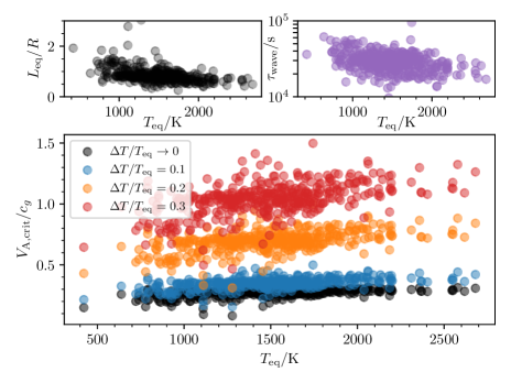
Figure 1: $L_{\mathrm{eq}}/R$ (top left), $\tau_{\mathrm{wave}}$ (top right), and $V_{\mathrm{A},\mathrm{crit}}/c_{g}$ (bottom panel) vs. $T_{\mathrm{eq}}$, using the exoplanet.eu dataset, where $V_{\mathrm{A},\mathrm{crit}}/c_{g}$ is calculated for $\Delta T/T_{\mathrm{eq}}=\{0,0.1,0.2,0.3\}$.

3 Method for Placing Magnetic Reversal Criteria on hot Jupiters

Equation 1 shows that the parameters $R$, $c_{g}$, $\Omega$, $\tau_{\mathrm{rad}}$, and $\Delta h_{\mathrm{eq}}/H$ can be used to estimate the minimum magnetic field strengths required for reversals. We apply this simple relation to a dataset of HJs taken from exoplanet.eu, using planets with $0.1\,M_{\mathrm{J}}<M<10\,M_{\mathrm{J}}$ and $a<0.1\,\mathrm{AU}$, where $M$ and $M_{\mathrm{J}}$ denote the planetary mass and Jupiter’s mass respectively, and $a$ is the semimajor axis. The criteria are calculated using the equilibrium temperature (assuming zero albedos; e.g., Laughlin et al., 2011):

$$T_{\mathrm{eq}}=\left(\frac{R_{*}}{2a}\right)^{1/2}\frac{T_{*}}{(1-e^{2})^{1/8}},$$ (2)

for stellar radius, $R_{*}$, orbital eccentricity, $e$, and stellar effective temperature, $T_{*}$.

The validity of the shallow-water approximation can be assessed by comparing $L_{\mathrm{eq}}$ to the pressure scale height, $H\sim\mathcal{R}T_{\mathrm{eq}}R^{2}/GM$, where $G$ is Newton’s gravitational constant and $\mathcal{R}$, the specific gas constant, is calculated using the solar system abundances in Lodders (2010). For the sampled HJs, $\mathrm{mean}(H/L_{\mathrm{eq}})=$7.5\text{\times}{10}^{-3}$$, so shallow-water theory is generally expected to capture their leading order atmospheric dynamics well. The shallow-water gravity wave speed is calculated by equating thermal and geopotential energies, yielding $c_{g}\equiv\sqrt{gH}\sim(\mathcal{R}T_{\mathrm{eq}})^{1/2}$. Doing so implies $\Delta h/H\sim\Delta T/T_{\mathrm{eq}}$, where $\Delta h$ are deviations in shallow-water layer thickness from the reference $H$ and $\Delta T\equiv T_{\mathrm{day}}-T_{\mathrm{eq}}$ for the dayside temperature, $T_{\mathrm{day}}$. Though not exactly equal, $\tau_{\mathrm{rad}}\sim\tau_{\mathrm{wave}}$ in the upper atmospheres of hot Jupiters (Fortney et al., 2008; Rogers & Komacek, 2014; Rogers, 2017). Taking $\tau_{\mathrm{rad}}=\tau_{\mathrm{wave}}$ is also convenient for this analysis as, when $\tau_{\mathrm{rad}}\lesssim\tau_{\mathrm{wave}}$, $\Delta h\sim\Delta h_{\mathrm{eq}}$ (Perez-Becker & Showman, 2013; Hindle et al., 2021), so $\Delta h_{\mathrm{eq}}/H\sim\Delta T/T_{\mathrm{eq}}$. While this treatment is a dynamic simplification, in Hindle et al. (2021) we found that it predicts reversal criteria consistent with the 3D MHD simulations of Rogers & Komacek (2014) and Rogers (2017).

An interesting feature of HJs is that the dynamical parameters $c_{g}$, $\Omega$ and $R$ of a HJ are all related to its host star proximity and the mass/radius/luminosity of its host star (i.e., they are all related to $T_{\mathrm{eq}}$). The consequence of this interdependence is that, for the hottest HJs, $L_{\mathrm{eq}}/R$ and $\tau_{\mathrm{wave}}$ approximately converge to $L_{\mathrm{eq}}/R\approx 0.7$ and $\tau_{\mathrm{wave}}\approx 2\times 10^{4}\,\mathrm{s}$ (see Figure 1; top panels). In Figure 1 (bottom panel) we use Equation 1 to plot $V_{\mathrm{A},\mathrm{crit}}/c_{g}$ for $\Delta T/T_{\mathrm{eq}}=0,0.1,0.2,0.3$. Taking $\Delta T\approx(T_{\mathrm{day}}-T_{\mathrm{night}})/2$, $\Delta T/T_{\mathrm{eq}}=0.1,0.2,0.3$ cover the expected range of relative dayside-nightside variations (e.g., Komacek et al., 2017); whereas $\Delta T/T_{\mathrm{eq}}=0$ shows the zero-amplitude limit. $V_{\mathrm{A},\mathrm{crit}}/c_{g}$ varies linearly with $\Delta T/T_{\mathrm{eq}}$ above $\Delta T/T_{\mathrm{eq}}=0.1$, but approaches the zero-amplitude limit for $\Delta T/T_{\mathrm{eq}}\lesssim 0.1$. A remarkable feature of the HJ dataset is that, due to the aforementioned interdependences, the ratio $V_{\mathrm{A},\mathrm{crit}}/c_{g}$ also converges in the large $T_{\mathrm{eq}}$ limit for a given $\Delta T/T_{\mathrm{eq}}$.

Equation 1, the Alfvén speed definition, and the ideal gas law yield

$$B_{\phi,\mathrm{crit}}=\left(\frac{\mu_{0}P}{\mathcal{R}T}\right)^{1/2}V_{\mathrm{A},\mathrm{crit}}\sim\frac{V_{\mathrm{A},\mathrm{crit}}}{c_{g}}\sqrt{\mu_{0}P}\ ,$$ (3)

where $B_{\phi,\mathrm{crit}}$ is the critical threshold of the toroidal field magnitude $B_{\phi}$, $\mu_{0}$ is the permeability of free space, and $T$ and $P$ are the temperature and pressure at which the reversal occurs.

If the electric currents that generate the planet’s assumed deep-seated dipolar field are located far below the atmosphere, Menou (2012) showed that $B_{\phi}$ can be related to the dipolar field strength, $B_{\mathrm{dip}}$, by the scaling law

$$B_{\phi}\sim R_{m}B_{\mathrm{dip}},$$ (4)

where $R_{m}={U_{\phi}H}/{\eta}$ is the magnetic Reynolds number for a given magnetic diffusivity, $\eta$, zonal wind speed, $U_{\phi}$, and pressure scale height, $H$. $R_{m}$ estimates the relative importance of the atmospheric toroidal field’s induction and diffusion; while $U_{\phi}/c_{g}$ scales linearly with $\Delta h/H\sim\Delta T/T_{\mathrm{eq}}$ in geostrophically or drag dominated flows (Perez-Becker & Showman, 2013). Taking a geostrophically-dominated flow yields $fU_{\phi}\sim(\Delta T/T_{\mathrm{eq}})c_{g}^{2}/L_{\mathrm{eq}}$, so $U_{\phi}/c_{g}\sim(\Delta T/T_{\mathrm{eq}})L_{D}/L_{\mathrm{eq}}$, with $L_{D}=c_{g}/f$. We fix the constant of proportionality in this scaling by setting $U_{\phi}\sim 1.5\times 10^{2}\,\mathrm{m}\,\mathrm{s}^{-1}$ for the conditions corresponding to the simulations of Rogers (2017). We calculate $\eta$ following the method of Rauscher & Menou (2013) and Rogers & Komacek (2014), taking

$$\eta=230\times 10^{-4}\,\frac{\sqrt{T}}{\chi_{e}}\,\mathrm{m}^{2}\,\mathrm{s}^{-1},$$ (5)

where $\chi_{e}$ is the ionisation fraction, which is calculated using a form of the Saha equation that takes into account all elements from hydrogen to nickel. It is given by

$$\chi_{e}=\sum_{i=1}^{28}\left(\frac{n_{i}}{n}\right)\chi_{e,i}\,.$$ (6)

In this sum the number density for each element, $n_{i}$, and the ionisation fraction of each element, $\chi_{e,i}$, are calculated using

$$n_{i}=n\left(\frac{a_{i}}{a_{H}}\right)=\frac{\rho}{\mu_{m}}\left(\frac{a_{i}}{a_{H}}\right),$$ (7)

$$\frac{\chi_{e,i}^{2}}{1-\chi_{e,i}^{2}}= n_{i}^{-1}\left(\frac{2\pi m_{e}}{h^{2}}\right)^{3/2}(kT)^{3/2}\exp\left(-\frac{\epsilon_{i}}{kT}\right),$$ (8)

for density $\rho$, total number density $n$, molecular mass $\mu_{m}$, relative elemental abundance (normalised to the hydrogen abundance) $a_{i}/a_{H}$, the electron mass $m_{e}$, Plank’s constant $h$, the Boltzmann constant $k$, and the elemental ionisation potential $\epsilon_{i}$. To calculate $\eta$, we use the solar system abundances in Lodders (2010) and take $T=T_{\mathrm{eq}}+\Delta T/\sqrt{2}$, the root-mean-squared temperature for a sinusoidal longitudinal temperature profile.

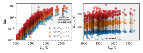
Figure 2: $R_{m}$ (left) and $B_{\phi,\mathrm{crit}}$ (right) vs. $T_{\mathrm{eq}}$, for the exoplanet.eu dataset. The estimates are calculated at $P=10\,\mathrm{mbar}$ with $T=T_{\mathrm{eq}}+\Delta T$, where $\Delta T/T_{\mathrm{eq}}=0.1,0.2,0.3$ (blue, orange, red). For each HJ, these are connected by a translucent line. The dashed reference lines $T_{\mathrm{eq}}=1500\,\mathrm{K}$ and $R_{m}=1$ (lefthand panel only) are also overplotted.

4 Magnetic field constraints

4.1 Estimates of $R_{m}$ and $B_{\phi,\mathrm{crit}}$

Estimates of $R_{m}$ and $B_{\phi,\mathrm{crit}}$ are calculated at depths corresponding to $P=10\,\mathrm{mbar}$, at which Rogers & Komacek (2014) found magnetically-driven wind variations. In Figure 2 we plot $R_{m}$ (lefthand panel) and $B_{\phi,\mathrm{crit}}$ (righthand panel) vs. $T_{\mathrm{eq}}$, for HJs in the dataset (with $T_{\mathrm{eq}}>1000\,\mathrm{K}$), taking $\Delta T/T_{\mathrm{eq}}=0.1,0.2,0.3$.

Induction of the atmospheric toroidal field is expected to become significant when $R_{m}$ exceeds unity. At $P=10\,\mathrm{mbar}$, $R_{m}$ exceeds unity for $T\gtrsim 1500\,\mathrm{K}$, depending on $\Delta T/T_{\mathrm{eq}}$. However, due to the highly temperature dependent nature of Equation 8, $R_{m}$ varies significantly when one compares $\Delta T/T_{\mathrm{eq}}=0.1,0.3$ for a given HJ.

As we see in Section 4.2, $B_{\phi}$ is only likely to exceed $B_{\phi,\mathrm{crit}}$ if the HJ in question is hot enough to maintain a significant atmospheric toroidal field ($R_{m}\gg 1$). We therefore concentrate our discussion on these hotter HJs; however, we place hypothetical estimates on $B_{\phi,\mathrm{crit}}$ for all planets in the dataset with $T_{\mathrm{eq}}>1000\,\mathrm{K}$ (Figure 2, righthand panel). Since, for a given $\Delta T/T_{\mathrm{eq}}$, $V_{\mathrm{A},\mathrm{crit}}/c_{g}$ is virtually independent of $T_{\mathrm{eq}}$ in the hottest HJs, so is $B_{\phi,\mathrm{crit}}$, with $100\,\mathrm{G}\lesssim B_{\phi,\mathrm{crit}}\lesssim 450\,\mathrm{G}$ for $0.1<\Delta T/T_{\mathrm{eq}}<0.3$; whereas larger $L_{\mathrm{eq}}/R$ values can cause $B_{\phi,\mathrm{crit}}$ to decrease in the cooler HJs (compare with Figure 1). We comment that $B_{\phi,\mathrm{crit}}$ is generally least severe in the uppermost regions of the atmosphere, where the atmosphere is least dense, explaining why Rogers & Komacek (2014) found the east-west wind variations at these depths.

In Hindle et al. (2021), we highlighted that magnetically-driven wind variations can be viewed as a saturation mechanism for the atmospheric toroidal field, with the reversal mechanism preventing $B_{\phi}$ from greatly exceeding $B_{\phi,\mathrm{crit}}$. This suggests that $B_{\phi}$ should peak in the deepest regions satisfying $B_{\phi}\sim B_{\phi,\mathrm{crit}}$, where $B_{\phi,\mathrm{crit}}$ can be large, then decrease towards the surface, where $B_{\phi,\mathrm{crit}}$ is smaller. This is consistent with Rogers & Komacek (2014), who found $B_{\phi}$ peaks in the mid-atmosphere (and declined to $300\,\mathrm{G}\lesssim B_{\phi}\lesssim 450\,\mathrm{G}$ at $P=10\,\mathrm{mbar}$ in their M7b simulations).

4.2 Dipolar magnetic field strengths

In Figure 3 we use Equation 4 to plot $T_{\mathrm{eq}}$ vs. $B_{\mathrm{dip},\mathrm{crit}}$, the critical dipolar field (at $P=10\,\mathrm{mbar}$) for $\Delta T/T_{\mathrm{eq}}=0.1,0.2,0.3$. Since the translation of planetary dynamo theory into the HJ parameter regime is not well-understood, we include a physically motivated reference line at $B_{\mathrm{dip},\mathrm{crit}}=14\,\mathrm{G}$ (the magnitude of Jupiter’s magnetic field at its polar surface) and a second reference line at $28\,\mathrm{G}$ (twice this). Due to the highly temperature dependent nature of $R_{m}$, these estimates of $B_{\mathrm{dip},\mathrm{crit}}$ carry a high degree of uncertainty (e.g., compare $B_{\mathrm{dip},\mathrm{crit}}$ of a given HJ for the different $\Delta T/T_{\mathrm{eq}}$ choices). Therefore, for useful estimates of $B_{\mathrm{dip},\mathrm{crit}}$, accurate temperature estimates/measurements (at the depth being probed) are required.

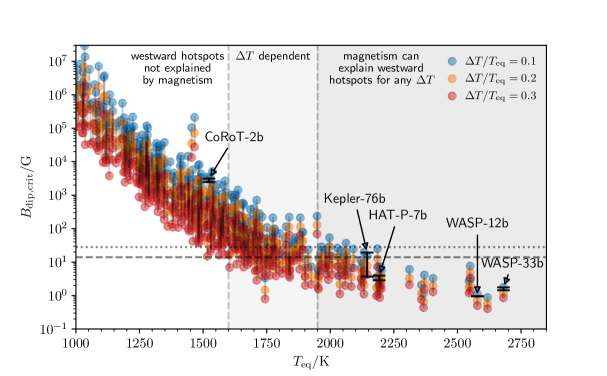
Figure 3: Critical dipole magnetic field strengths, $B_{\mathrm{dip},\mathrm{crit}}$, at $P=10\,\mathrm{mbar}$. We plot $B_{\mathrm{dip},\mathrm{crit}}$ using $T=T_{\mathrm{eq}}+\Delta T$, with $\Delta T/T_{\mathrm{eq}}=0.1,0.2,0.3$ (blue, orange, red). For a given HJ, these are connected by translucent lines. We include error bars and labels for the planets discussed in this letter (see Table 1) along with reference lines at $14\,\mathrm{G}$ (dashed; Jupiter’s polar surface magnetic field strength) and $28\,\mathrm{G}$ (dotted; twice this).

Generally, $T_{\mathrm{day}}$ is not directly calculable from standard planetary/stellar parameters, so measured values should be used where possible. For the five HJs with westward hotspot observations, we use dayside temperatures based on phase curve measurements to estimate $B_{\phi,\mathrm{crit}}$ and $B_{\mathrm{dip},\mathrm{crit}}$. We present these estimates in Table 1 and add labelled error bars to Figure 3. The UHJs are found to have low-to-moderate $B_{\mathrm{dip},\mathrm{crit}}$ requirements. For HAT-P-7b we estimate $3\,\mathrm{G}<B_{\mathrm{dip},\mathrm{crit}}<4\,\mathrm{G}$ at $P=10\,\mathrm{mbar}$, recovering the previously-known result that westward hotspots on HAT-P-7b can be well-explained by magnetism (Rogers, 2017; Hindle et al., 2019). On the UHJs WASP-12b and WASP-33b dipole fields respectively exceeding $1\,\mathrm{G}$ and $2\,\mathrm{G}$ at $P=10\,\mathrm{mbar}$ would explain westward hotspots. Likewise, at $P=10\,\mathrm{mbar}$, a dipole field exceeding $B_{\mathrm{dip},\mathrm{crit}}$ for $4\,\mathrm{G}<B_{\mathrm{dip},\mathrm{crit}}<19\,\mathrm{G}$ is required to explain westward hotspots on Kepler-76b. Given the comparison with Jupiter and that Cauley et al. (2019) predicted surface magnetic fields on HJs could range from $20\,\mathrm{G}$ to $120\,\mathrm{G}$, these estimates support the idea that wind reversals on these UHJs have a magnetic origin. If non-magnetic explanations can be ruled out, such estimates of $B_{\mathrm{dip},\mathrm{crit}}$ can be used as lower bounds for $B_{\mathrm{dip}}$ on UHJs. In contrast, unless CoRoT-2b hosts an unfeasibly large $\gtrsim 3\,\mathrm{kG}$ dipolar field, its westward hotspots are not explained by magnetism (recovering the result of Hindle et al., 2019). To check our method’s fidelity, we also compare predictions to the simulations in Rogers & Komacek (2014), finding good agreement (for both $B_{\mathrm{dip},\mathrm{crit}}$ and $B_{\mathrm{\phi},\mathrm{crit}}$).

Using the range $\Delta T/T_{\mathrm{eq}}=(0.1,0.3)$ to estimate $B_{\mathrm{\phi},\mathrm{crit}}$ generally has uncertainties between one-half and one order of magnitude. However, Figure 3 shows that HJs divide into three clear categories: (i) those likely to have magnetically-driven atmospheric wind variations for any choice of $\Delta T/T_{\mathrm{eq}}$ ($T_{\mathrm{eq}}\gtrsim 1950\,\mathrm{K}$); (ii) those unlikely to have sufficiently strong toroidal fields to explain atmospheric wind variations, for any choice of $\Delta T/T_{\mathrm{eq}}$ ($T_{\mathrm{eq}}\ll 1600\,\mathrm{K}$); and (iii) marginal cases that depend on the magnitude of day-night temperature differences ($1600\,\mathrm{K}\lesssim T_{\mathrm{eq}}\lesssim 1950\,\mathrm{K}$).

Using the conditions $B_{\mathrm{dip},\mathrm{crit}}<28\,\mathrm{G}$, $P=10\,\mathrm{mbar}$, and $\Delta T/T_{\mathrm{eq}}=0.1$, we identify 61 further HJs that are likely to exhibit magnetically-driven wind variations. We present these in Table 2 (Appendix A), which is ordered by ascending $B_{\mathrm{dip},\mathrm{crit}}$ (i.e., from most-likely to least-likely to exhibit reversals), to help guide future observational missions. Of these 61 reversal candidates, 37 HJs have weaker reversal requirements than Kepler-76b. Hence, using these fairly conservative criteria, we predict that magnetic wind variations could be present in $\sim 60$ and argue that they are highly-likely in $\sim 40$ of the hottest HJs.

For HJs with intermediate temperatures ($1600\,\mathrm{K}\lesssim T_{\mathrm{eq}}\lesssim 1950\,\mathrm{K}$), the magnitude of $\Delta T/T_{\mathrm{eq}}$ (and our simplifying assumptions) plays a significant role in determining whether magnetic wind variations are plausible, so specific dayside temperature measurements should be used for estimates. These intermediate temperatures HJs offer excellent opportunities to fine-tune magnetohydrodynamic theory, via cross-comparisons between observations and bespoke models.

Table 1: Estimates of $B_{\phi,\mathrm{crit}}$ and $B_{\mathrm{dip},\mathrm{crit}}$ at $P=10\,\mathrm{mbar}$, using the tabulated $T_{\mathrm{day}}$, for HAT-P-7b, CoRoT-2b, Kepler-76b, WASP-12b, and WASP-33b.

Planet	$T_{\mathrm{day}}/\,\mathrm{K}$	$B_{\phi,\mathrm{crit}}/\,\mathrm{G}$	$B_{\mathrm{dip},\mathrm{crit}}/\,\mathrm{G}$
HAT-P-7b	$(2610,2724)^{1}$	$(255,324)$	$(3,4)$
CoRoT-2b	$(1695,1709)^{2}$	$(145,177)$	$(2500,3100)$
Kepler-76b	$(2300,2850)^{3}$	$(107,466)$	$(4,19)$
WASP-12b	$(2928)^{4}$	$(212)$	$(0.9)$
WASP-33b	$(2954,3074)^{5}$	$(152,218)$	$(1.4,1.8)$

5 Discussion

We have applied the theory developed in Hindle et al. (2021) to a dataset of HJs to estimate the critical magnetic field strengths $B_{\mathrm{dip},\mathrm{crit}}$ and $B_{\phi,\mathrm{crit}}$ (at $P=10\,\mathrm{mbar}$), beyond which strong toroidal fields cause westward hotspots. The new criterion differs both mathematically and in physical interpretation from the criterion of Rogers & Komacek (2014) and Rogers (2017), which identifies when Lorentz forces from the deep-seated dipolar field become strong enough to significantly reduce zonal winds, but doesn’t theoretically explain wind variations. However, the estimates made in this work match well with typical magnetic fields in the 3D simulations of Rogers & Komacek (2014) and Rogers (2017), which exhibit wind variations, and also match values resulting from their criterion in these regions of parameter space. This is because, while describing different magnetic effects, both criteria predict the critical magnetic field strengths at which magnetism becomes dynamically-important in HJ atmospheres. Applying the new criterion to the HJ dataset, we found that the brightspot variations on Kepler-76b can be explained by plausible planetary dipole strengths ($B_{\mathrm{dip}}\gtrsim 4\,\mathrm{G}$ using $T_{\mathrm{day}}=2850$; $B_{\mathrm{dip}}\gtrsim 19\,\mathrm{G}$ using $T_{\mathrm{day}}=2300$), and that westward hotspots can be explained for $B_{\mathrm{dip}}\gtrsim 1\,\mathrm{G}$ on WASP-12b and $B_{\mathrm{dip}}\gtrsim 2\,\mathrm{G}$ on WASP-33b. The estimates of $B_{\phi,\mathrm{crit}}$ and $B_{\mathrm{dip},\mathrm{crit}}$ for HAT-P-7b and CoRoT-2b are consistent with the estimates of Rogers (2017) and Hindle et al. (2019). We then used an observationally motivated set of criteria ($B_{\mathrm{dip},\mathrm{crit}}<28\,\mathrm{G}$, $\Delta T/T_{\mathrm{eq}}=0.1$, and $P=10\,\mathrm{mbar}$) to tabulate 65 HJs that are likely to exhibit magnetically-driven wind variations (see LABEL:{tab:reversal:HJs}, Appendix A) and predict such effects are highly-likely in $\sim 40$ of the hottest HJs.

With exoplanet meteorology becoming increasingly developed, the results of this study suggests that further observations of hotspot variations in UHJs should be expected. A combination of archival data and future dedicated observational missions from Kepler, Spitzer, Hubble, TESS, CHEOPS, and JWST can be used to identify magnetically-driven wind variations and other interesting features at different atmospheric depths. In particular, long time-span studies observing multiple transits of UHJs are likely to be essential in understanding hotspot/brightspot oscillations. Of the studies that have measured westward hotspot/brightspot offets, only the long time-span studies of Armstrong et al. (2016) (HAT-P-7b; 4 years) and Jackson et al. (2019) (Kepler-76b; 1000 days) identify hotspot/brightspot oscillations. In both cases, such oscillations are observed on timescales of $\sim$$10$-$100\mbox{ Earth days}$, which Rogers (2017) noted is consistent with timescales of wind variability in 3D MHD simulations (and the deep-seated magnetic field’s Alfvén timescale). Such timescales are of-order or longer than the total time-spans of the other UHJ studies with westward hotspot/brightspot measurements (Bell et al., 2019; von Essen et al., 2020), so it is impossible to tell whether these measurements are part of an oscillatory evolution.

If non-magnetic explanations can be ruled-out for past and future identifications of westward hotspot offsets on UHJs, the coolest planets with wind variations can indicate typical $B_{\mathrm{dip}}$ magnitudes on HJs. This has the potential to drive new understanding of the atmospheric dynamics of UHJs and provide important observational constraints for dynamo models of HJs. Parallel to this, future theoretical work can refine estimates of $B_{\mathrm{dip},\mathrm{crit}}$. In many cases combining observational measurements with bespoke 3D MHD simulations offer the best prospect for providing accurate constraints on the magnetic field strengths of UHJs, yet the simple concepts and results of this work can provide useful starting points for such studies and can highlight trends from an ensemble viewpoint. The largest limiting factor in our estimates of $B_{\mathrm{dip},\mathrm{crit}}$ is the highly temperature dependent nature of $R_{m}$. Furthermore, the magnetic scaling law does not account for longitudinal asymmetries in the magnetic diffusivity or the dipolar field strength within the atmospheric region. In future work we shall investigate how these inhomogeneities effect the atmospheric dynamics more closely, using a 3D model containing variable magnetic diffusivity, consistent poloidal-toroidal field coupling, stratification, and thermodynamics. To date, MHD models of HJs have strictly considered dipolar magnetic field geometries for the planetary magnetic field. Dynamo simulations would offer insight into the nature of magnetic fields in the deep interiors of HJs, which, at present, is not well-understood.

Appendix A Candidate hot Jupiters for magnetically-driven wind variations

Table 2: HJs in which $B_{\mathrm{dip},\mathrm{crit}}<28\,\mathrm{G}$, at $P=10\,\mathrm{mbar}$ with $\Delta T/T_{\mathrm{eq}}=0.1$. Alongside $T_{\mathrm{eq}}$, estimates of $B_{\mathrm{dip},\mathrm{crit}}$ and $B_{\mathrm{dip},\mathrm{crit}}$ are provided for these choices.

Rank	Candidate	$T_{\mathrm{eq}}/\mathrm{K}$	$B_{\phi,\mathrm{crit},0.1}/\mathrm{G}$	$B_{\mathrm{dip},\mathrm{crit},0.1}/\mathrm{G}$
1	WASP-189 b	2618	129	0.9
2†	$\dagger\quad$ WASP-12 b	2578	156	1
3	WASP-178 b	2366	130	1
4†	$\dagger\quad$ WASP-33 b	2681	149	2
5	WASP-121 b	2358	153	2
6	MASCARA-1 b	2545	134	3
7	WASP-78 b	2194	139	3
8	HAT-P-70 b	2551	133	3
9	HD 85628 A b	2403	128	3
10	HATS-68 b	1743	177	3
11	WASP-76 b	2182	145	3
12	WASP-82 b	2188	132	4
13	HD 202772 A b	2132	125	4
14	Kepler-91 b	2037	105	4
15	TOI-1431 b/MASCARA-5 b	2370	129	4
16	HAT-P-65 b	1953	138	5
17	WASP-100 b	2201	131	6
18	WASP-187 b	1952	116	6
19	HATS-67 b	2195	146	6
20	WASP-87 A b	2311	139	6
21	HATS-56 b	1902	122	7
22	HATS-40 b	2121	126	7
23	KELT-18 b	2082	130	7
24	HAT-P-57 b	2198	130	7
25	HATS-26 b	1925	130	7
26†	$\dagger\quad$ HAT-P-7 b	2192	134	7
27	WASP-48 b	2058	139	7
28	KOI-13 b	2550	139	8
29	HAT-P-49 b	2127	128	9
30	WASP-142 b	1992	139	11
31	WASP-111 b	2121	133	11
32	WASP-90 b	1840	124	12
33	HAT-P-66 b	1900	130	12
34	Qatar-10 b	1955	145	13
35	KELT-11 b	1711	113	13
36	HAT-P-33 b	1839	130	14
37	HATS-35 b	2033	140	14
38	HAT-P-60 b	1786	119	15
39	Qatar-7 b	2052	141	15
40	CoRoT-1 b	2007	146	15
41†	$\dagger\quad$ Kepler-76 b	2145	142	15
42	K2-260 b	1985	132	15
43	WASP-71 b	2064	128	15
44	WASP-88 b	1763	119	16
45	WASP-172 b	1745	114	16
46	WASP-159 b	1811	120	17
47	Kepler-435 b	1731	109	18
48	HATS-31 b	1837	128	19
49	WASP-122 b	1962	147	19
50	HAT-P-32 b	1841	142	19
51	HAT-P-23 b	2133	148	20
52	WASP-92 b	1879	137	20
53	HATS-64 b	1800	119	21
54	WASP-19 b	2060	160	21
55	KELT-4 A b	1827	133	21
56	CoRoT-21 b	2041	126	22
57	HATS-9 b	1913	135	23
58	HAT-P-69 b	1980	118	23
59	OGLE-TR-132 b	1981	138	24
60	HATS-24 b	2091	148	25
61	Kepler-1658 b	2185	110	25
62	TOI-954 b	1704	109	26
63	WASP-114 b	2028	142	26
64	TOI-640 b	1749	120	27
65	WASP-153 b	1712	128	27

References

- Armstrong et al. (2016) Armstrong, D. J., de Mooij, E., Barstow, J., et al. 2016, NatAs, 1, 0004, doi: 10.1038/s41550-016-0004
- Bell et al. (2019) Bell, T. J., Zhang, M., Cubillos, P. E., et al. 2019, MNRAS, 489, 1995, doi: 10.1093/mnras/stz2018
- Cauley et al. (2019) Cauley, P. W., Shkolnik, E. L., Llama, J., & Lanza, A. F. 2019, Nature Astronomy, 3, 1128, doi: 10.1038/s41550-019-0840-x
- Cooper & Showman (2005) Cooper, C. S., & Showman, A. P. 2005, ApJ, 629, L45, doi: 10.1086/444354
- Cooper & Showman (2006) —. 2006, ApJ, 649, 1048, doi: 10.1086/506312
- Cowan et al. (2007) Cowan, N. B., Agol, E., & Charbonneau, D. 2007, MNRAS, 379, 641, doi: 10.1111/j.1365-2966.2007.11897.x
- Cowan et al. (2012) Cowan, N. B., Machalek, P., Croll, B., et al. 2012, ApJ, 747, 82, doi: 10.1088/0004-637X/747/1/82
- Dang et al. (2018) Dang, L., Cowan, N. B., Schwartz, J. C., et al. 2018, NatAs, 2, 220, doi: 10.1038/s41550-017-0351-6
- Demory et al. (2013) Demory, B.-O., de Wit, J., Lewis, N., et al. 2013, ApJ, 776, L25, doi: 10.1088/2041-8205/776/2/L25
- Fortney et al. (2008) Fortney, J. J., Lodders, K., Marley, M. S., & Freedman, R. S. 2008, ApJ, 678, 1419, doi: 10.1086/528370
- Harrington et al. (2006) Harrington, J., Hansen, B. M., Luszcz, S. H., et al. 2006, Science, 314, 623, doi: 10.1126/science.1133904
- Helling et al. (2019) Helling, C., Iro, N., Corrales, L., et al. 2019, A&A, 631, A79, doi: 10.1051/0004-6361/201935771
- Hindle et al. (2019) Hindle, A. W., Bushby, P. J., & Rogers, T. M. 2019, ApJ, 872, L27, doi: 10.3847/2041-8213/ab05dd
- Hindle et al. (2021) —. 2021, arXiv e-prints, arXiv:2107.07515. https://arxiv.org/abs/2107.07515
- Jackson et al. (2019) Jackson, B., Adams, E., Sandidge, W., Kreyche, S., & Briggs, J. 2019, AJ, 157, 239, doi: 10.3847/1538-3881/ab1b30
- Knutson et al. (2007) Knutson, H. A., Charbonneau, D., Allen, L. E., et al. 2007, Nature, 447, 183, doi: 10.1038/nature05782
- Knutson et al. (2009) Knutson, H. A., Charbonneau, D., Cowan, N. B., et al. 2009, ApJ, 690, 822, doi: 10.1088/0004-637X/690/1/822
- Komacek et al. (2017) Komacek, T. D., Showman, A. P., & Tan, X. 2017, ApJ, 835, 198, doi: 10.3847/1538-4357/835/2/198
- Laughlin et al. (2011) Laughlin, G., Crismani, M., & Adams, F. C. 2011, ApJ, 729, L7, doi: 10.1088/2041-8205/729/1/l7
- Lee et al. (2016) Lee, G., Dobbs-Dixon, I., Helling, C., Bognar, K., & Woitke, P. 2016, A&A, 594, A48, doi: 10.1051/0004-6361/201628606
- Lodders (2010) Lodders, K. 2010, in Principles and Perspectives in Cosmochemistry, ed. A. Goswami & B. E. Reddy (Berlin, Heidelberg: Springer Berlin Heidelberg), 379–417
- Menou (2012) Menou, K. 2012, ApJ, 745, 138, doi: 10.1088/0004-637X/745/2/138
- Parmentier et al. (2016) Parmentier, V., Fortney, J. J., Showman, A. P., Morley, C., & Marley, M. S. 2016, ApJ, 828, 22, doi: 10.3847/0004-637X/828/1/22
- Perez-Becker & Showman (2013) Perez-Becker, D., & Showman, A. P. 2013, ApJ, 776, 134, doi: 10.1088/0004-637X/776/2/134
- Rauscher & Kempton (2014) Rauscher, E., & Kempton, E. M. R. 2014, ApJ, 790, 79, doi: 10.1088/0004-637X/790/1/79
- Rauscher & Menou (2013) Rauscher, E., & Menou, K. 2013, The Astrophysical Journal, 764, 103, doi: 10.1088/0004-637x/764/1/103
- Rogers (2017) Rogers, T. M. 2017, NatAs, 1, 0131, doi: 10.1038/s41550-017-0131
- Rogers & Komacek (2014) Rogers, T. M., & Komacek, T. D. 2014, ApJ, 794, 132, doi: 10.1088/0004-637X/794/2/132
- Shell & Held (2004) Shell, K. M., & Held, I. M. 2004, Journal of Atmospheric Sciences, 61, 2928, doi: 10.1175/JAS-3312.1
- Showman & Guillot (2002) Showman, A. P., & Guillot, T. 2002, A&A, 385, 166, doi: 10.1051/0004-6361:20020101
- Showman & Polvani (2011) Showman, A. P., & Polvani, L. M. 2011, ApJ, 738, 71, doi: 10.1088/0004-637X/738/1/71
- von Essen et al. (2020) von Essen, C., Mallonn, M., Borre, C. C., et al. 2020, A&A, 639, A34, doi: 10.1051/0004-6361/202037905
- Wong et al. (2016) Wong, I., Knutson, H. A., Kataria, T., et al. 2016, ApJ, 823, 122, doi: 10.3847/0004-637X/823/2/122