Accelerating Quadratic Optimization
with Reinforcement Learning

Abstract

First-order methods for quadratic optimization such as OSQP are widely used for large-scale machine learning and embedded optimal control, where many related problems must be rapidly solved. These methods face two persistent challenges: manual hyperparameter tuning and convergence time to high-accuracy solutions. To address these, we explore how Reinforcement Learning (RL) can learn a policy to tune parameters to accelerate convergence. In experiments with well-known QP benchmarks we find that our RL policy, RLQP, significantly outperforms state-of-the-art QP solvers by up to 3x. RLQP generalizes surprisingly well to previously unseen problems with varying dimension and structure from different applications, including the QPLIB, Netlib LP and Maros-Mészáros problems. Code for RLQP is available at https://github.com/berkeleyautomation/rlqp.

1 Introduction

Solving quadratic programs (QPs) efficiently is critical to applications in finance, robotic control and operations research. While state-of-the-art interior-point methods scale poorly with problem dimensions, first-order methods for solving QPs typically require thousands of iterations. Moreover, real-time control applications have tight latency constraints for solvers [34]. Therefore, it is important to develop efficient heuristics to solve QPs in fewer iterations.

The Alternating Direction Method of Multipliers (ADMM) [6, 16, 19] is an efficient first-order optimization algorithm, and is the basis for the widely used and state-of-the art Operator-Splitting QP (OSQP) solver [46]. ADMM performs a linear solve on a matrix based on the optimality conditions of the QP to generate a step direction, and then projects the step onto the constraint bounds.

While state-of-the-art, the ADMM algorithm has numerous hyperparameters that must be tuned with heuristics to regularize and control optimization. Most importantly, the step size parameter $\rho$ has considerable impact on the convergence rate. However, is still unclear how to select $\rho$ before attempting the QP solution. While some theoretical works compute the optimal $\rho$ [18], they rely on solving semidefinite optimization problems which are much harder than solving the QP itself. Alternatively, some heuristics introduce “feedback” by adapting $\rho$ throughout optimization in order to balance primal and dual residuals [46, 6, 23].

Figure 1: RLQP uses deep reinforcement learning (RL) to compute a policy that adapts the internal parameters of a first-order quadratic program (QP) solver to speed up the solver’s convergence rate. In a standard RL formulation, a policy computes an action based on its observation of the state of the environment, and taking the action results in a change in state and a reward. In RLQP, the policy is parameterized by a neural network, the state is the internal state of the QP solver, the action changes a parameter ($\rho$) of the solver, and the reward minimizes the time required to solve the QP.

We propose RLQP (see Fig. 1), an accelerated QP solver based on OSQP that uses reinforcement learning to adapt the internal parameters of the ADMM algorithm between iterations to minimize solve times. An RL algorithm learns a policy $\pi_{\theta}\colon\mathcal{S}\to\mathcal{A}$, parameterized by $\theta$ (e.g., the weights of a neural network), that maps states in a set $\mathcal{S}$ to actions in set $\mathcal{A}$ such that the selected action maximizes an accumulated reward $r$. To train the policy for RLQP, we define $\mathcal{S}$ to be the internal state of the QP solver (e.g., the constraint bounds, the primal and dual estimates), $\mathcal{A}$ to be the adaptation to the internal parameter ($\rho$) vector, and $r$ to minimize the number of ADMM iterations taken.

RLQP’s policy can be trained either jointly across general classes of QPs or with respect to a specific class. The general version of RLQP is trained once on a broad class of QPs and can be used out-of-the-box on new problems. The specialized version of RLQP is trained on a specific class of problems that the solver will repeatedly encounter. While this requires additional setup and training time, it is useful when QPs will be repeatedly solved in application (e.g., in a 100 Hz control loop).

In experiments, we train RLQP on a set of randomized QPs, and compare convergence rates of RLQP to non-adaptive and heuristic adaptive policies. To compare generalization and specialization, we investigate RLQP’s performance in the settings where 1) the train and test sets of QPs come from the same class of problems, 2) the train set contains from superset of classes contained in the test set, 3) the train set contains a subset, and 4) when the train and test sets are from distinct classes. In the results section we show that RLQP outperforms OSQP by up to 3x.

The contributions of this paper are:

• Two RL formulations to train policies that provide coarse (scalar) and fine (vector) grain updates to the internal parameters of a QP solver for faster convergence times

• Policies trained jointly across QP problem classes or to specialize to specific classes

• Experimental results showing that RLQP reduces convergence times by up to 3x and generalizes to different problem classes and outperform existing methods

2 Related Work

This work touches a number of related research areas, including convex optimization, using machine learning (ML) to speed up optimization, learning in first-order methods, and reinforcement learning.

Convex optimization

Many researchers have proposed algorithms for quadratic programs, which generally fall into three classes: active set [49], interior point [38], and first-order methods. Of the active set and interior point solvers, perhaps the most well-known are Gurobi [21] and MOSEK [37]. Active-set solvers operate by iteratively adapting an active set of constraints based on the cost function gradient and dual variables [40]. Interior-point solvers iteratively introduce and vary barrier functions to represent constraints and solve unconstrained convex problems. We instead base this work on a first-order method solver, OSQP [46]. One of the advantages of OSQP over interior points solvers, is that they can readily be warm started from a near-by solution, as is common in many applications such as solving a sequential quadratic program [43] and solving QPs for model-predictive control.

ML-accelerated combinatorial optimization

Accelerating combinatorial optimization problems with deep learning has been explored with wide application [4, 5], including branch-and-bound for mixed-integer linear programming [1, 28], graph algorithms [9] and boolean satisfiability problems (SAT) [7]. Many combinatorial optimization problems have exponential search spaces and are NP-hard in a general setting. However, learning-augmented combinatorial algorithms utilize very different methods to RLQP as combinatorial problems have discrete search spaces.

Learning in first-order methods

Accelerating first-order methods with machine learning has gained considerable recent interest. Li and Malik [29] demonstrate a learned optimization algorithm outperforms common first-order methods for several convex problems and a small non-convex problem. Metz et al. [35] show a learned policy outperforms first-order methods when optimizing neural networks, but finds that directly learning parameter update values can be sensitive to exploding gradient problems. We avoid this instability during optimization by learning a policy to adapt parameters of the ADMM algorithm. Wei et al. [48] recently proposed an RL agent to tune parameters for an ADMM-based inverse imaging solver.

Reinforcement Learning Overview

Reinforcement learning (RL) algorithms include both on-policy algorithms, such as Proximal Policy Optimization [44], REINFORCE [47], and IMPALA [12], and off-policy algorithms, such as DQN [36] and Soft Actor Critic [22]. RLQP extends the off-policy Twin-Delayed DDPG (TD3) [14], an actor-critic framework with a exploration policy for continuous action spaces that extends Deep Deterministic Policy Gradient (DDPG) algorithm [30] while addressing approximation errors. Furthermore, in one formulation of RLQP, we train a shared policy for multiple agents following an RL approach proposed by Huang et al. [24]. With this single policy, RLQP updates multiple parameters using state associated with each constraint of a QP.

3 Background

In this section, we summarize QPs, the OSQP solver, and a MDP formalization.

3.1 Quadratic Programs

A quadratic program with $n$ variables and $m$ constraints takes the form:

$$\begin{array}[]{ll}\mbox{minimize}&(1/2)x^{T}Px+q^{T}x\\ \mbox{subject to}&l\leq Ax\leq u,\end{array}$$

where ${x}\in\mathbb{R}^{n}$ is the optimization variable, ${P}$ is an $n\times n$ symmetric positive semi-definite matrix that defines the quadratic cost, ${q}\in\mathbb{R}^{n}$ defines the linear cost, ${A}$ is an $m\times n$ matrix that defines the $m$ linear constraints, and ${l},{u}\in\mathbb{R}^{m}$ are the constraint’s lower and upper bounds. Here, $\leq$ is an element-wise less-than-or-equal-to operator. In this form, to specify an equality constraint, the lower and upper bounds are set to the same value, and to specify a constraint unbounded from one side, a sufficiently large value (or $\pm\infty$) is specified for the other side.

3.2 First-Order QP Solver Algorithm

The solver we speed up is OSQP, which uses a first-order ADMM method to solve QPs. We summarize OSQP here. Given a QP, OSQP first forms a KKT matrix (below), then iteratively refines a solution from a initialization point for vectors ${x}^{(0)}\in\mathbb{R}^{n}$, ${y}^{(0)}\in\mathbb{R}^{m}$, and ${z}^{(0)}\in\mathbb{R}^{m}$, where the superscript in parenthesis refers to the iteration. Each iteration computes the values for the $k+1$ iterates by solving following linear system (e.g., with an $LDL^{T}$ solver):

$$\underbrace{\begin{bmatrix}P+\sigma I&A^{T}\\ A&\mathop{\mathrm{diag}}(\rho)^{-1}\end{bmatrix}}_{\text{KKT matrix}}\begin{bmatrix}x^{(k+1)}\\ v^{(k+1)}\end{bmatrix}\!=\!\begin{bmatrix}\sigma x^{(k)}-q\\ z^{(k)}-\mathop{\mathrm{diag}}(\rho)^{-1}y^{(k)}\end{bmatrix}$$ (1)

and then performing the following updates:

$$\tilde{{z}}^{(k+1)} \leftarrow{z}^{(k)}+\mathop{\mathrm{diag}}(\rho)^{-1}({v}^{(k+1)}-{y}^{(k)})$$

$$z^{(k+1)} \leftarrow\Pi\left(\tilde{z}^{(k+1)}+\mathop{\mathrm{diag}}(\rho)^{-1}y^{(k)}\right)$$

$$y^{(k+1)} \leftarrow x^{(k)}+\mathop{\mathrm{diag}}(\rho)\left(\tilde{z}^{(k+1)}-z^{(k+1)}\right),$$

where $\sigma\in\mathbb{R}_{+}$ and $\rho\in\mathbb{R}_{+}^{m}$ are regularization and step-size parameters, and $\Pi:\mathbb{R}^{m}\rightarrow\mathbb{R}^{m}$ projects its argument on the constraint bounds. We use the notation $\mathop{\mathrm{diag}}\colon\mathbb{R}^{m}\to\mathbb{S}^{m}$ to denote the operator that maps a vector to a diagonal matrix. We define the primal and the dual residual vectors as

$$\xi_{\rm primal}^{(k)}=Ax^{(k)}-b,\quad\mbox{and}\quad\xi_{\rm dual}^{(k)}=Px^{(k)}+q+A^{T}y^{(k)}.$$

When the primal and dual residual vectors are small enough in norm after $k$ iterations, $x^{(k+1)}$ and $y^{(k+1)}$ are primal and dual (approximate) solutions to the QP.

Internally, OSQP has a single scalar $\bar{\rho}$ that it uses to form $\rho$ according to the following formula:

$$\rho_{i}=\begin{cases}\bar{\rho}&\text{if }l_{i}\neq u_{i}\text{ (inequality constraints)}\\ \bar{\rho}\cdot 10^{3}&\text{if }l_{i}=u_{i}\text{ (equality constraints)},\end{cases}$$ (2)

where the subscript $i$ denotes the $i$-th coefficient of $\rho$, and the bounds ${l}$ and ${u}$.

Periodically, between ADMM iterations, OSQP will adapt the value of $\bar{\rho}$. The existing hand-crafted formula for adapting $\rho$ attempts to balance between primal and dual residuals, by setting $\bar{\rho}^{(k+1)}\leftarrow\bar{\rho}^{(k)}\sqrt{\|\xi_{\mathrm{primal}}\|/\|\xi_{\mathrm{dual}}\|}$. Empirically, adapting $\rho$ between iterations can speed up the convergence rate.

3.3 Multi-Agent Single-Policy MDP

In a Markov Decision Process (MDP), an agent can be in any state $s\in\mathcal{S}$, take an action $a\in\mathcal{A}$, and with the transition dynamics function, $\mathcal{T}(\cdot\mid s,a)$, transitions from state $s$ to state $s^{\prime}$ after taking action $a$. The agent receives a reward $R\colon\mathcal{S}\times\mathcal{A}\to\mathbb{R}$ for transitioning from $s$ to $s^{\prime}$ by taking action $a$. Given a tuple $(\mathcal{S},\mathcal{A},T,R,\gamma)$, the MDP optimization objective is to find a policy $\pi_{\theta}:\mathcal{S}\rightarrow\mathcal{A}$, parameterized by $\theta$, that maximizes the expected cumulative reward $E\left[\sum_{t=0}^{\infty}\gamma^{t}r^{t}\right],$ where $r^{t}$ is the reward at time $t$ and $\gamma\in[0,1)$ is a discount factor.

We also formulate a multi-agent single-policy MDP setting in which $m$ agents collaborate in a shared environment in state $s_{\mathrm{env}}\in\mathcal{S}_{\mathrm{env}}$. At each time step, each collaborating agent (CA) $i$ has its own state $s_{i}\in\mathcal{S}_{\mathrm{ca}}$, action $a_{i}\in\mathcal{A}_{\mathrm{ca}}$, and observations $o_{i}\in\mathcal{O}$, but, for computation feasibility, share a single policy $\pi_{\theta}:\mathcal{S}_{\mathrm{ca}}\rightarrow\mathcal{A}_{\mathrm{ca}}$. State transitions for the environment and all $m$ agents occur simultaneously according to a state transition function $\mathcal{T}:\mathcal{S}_{\mathrm{env}}\times\mathcal{S}_{\mathrm{ca}}^{m}\times\mathcal{A}_{\mathrm{ca}}^{m}\rightarrow\mathcal{S}_{\mathrm{env}}\times\mathcal{S_{\mathrm{ca}}}^{m}$ and result in a single shared reward $R:\mathcal{S}_{\mathrm{env}}\times\mathcal{S}_{\mathrm{ca}}^{m}\times\mathcal{A}_{\mathrm{ca}}^{m}\rightarrow\mathbb{R}$ and discount factor. The objective is to find a single shared policy $\pi_{\theta}$ that maximizes the expected cumulative reward. This can be thought of as a special case of a multi-agent MDP [32] or Markov game [31], and we adapt a formulation from Huang et al. [24].

4 Method

The goal of RLQP is to learn a policy to adapt the $\rho\in\mathbb{R}^{m}$ vector used in the ADMM update in (1) (see Fig. 1). As the dimensions of this vector vary between QPs, we propose two methods that can handle the variation in $m$. The first method learns a policy to adapt a scalar $\bar{\rho}$ and then applies (2) to populate the coefficients of the $\rho$ vector. The second method learns a policy to adapt individual coefficients of the $\rho$ vector.

Since both the number of variables $n$ and the number of constraints $m$ can vary from problem to problem, and the same QP can be written in $(n!\,m!)$ permutations, we propose learning policies that are problem size and permutation invariant. To do this, we provide a permutation-invariant fixed-size state of the QP solver to either policy.

4.1 RL Policy for Scalar Adaptation

Algorithm 1 TD3 for $\bar{\rho}$ (scalar)

1:  Input: exploration noise $\sigma$, buffer size $\mathtt{rs}$

2:  $\pi,Q\leftarrow$ initialize policy and critic (see TD3)

3:  $\mathcal{D}\leftarrow$ replay buffer w/ $\mathtt{rs}$

4:  $\mathtt{env},s^{(0)}\leftarrow$ new QP, its state

5:  for $t\in\{0,\ldots,T\}$ do

6:    ${\bar{\rho}}^{(t)}_{\phantom{i}}\leftarrow\pi(s^{(t)})+\epsilon$,   $\epsilon\sim\mathcal{N}(0,\sigma)$

7:    $s^{(t+1)},r^{(t)},\mathtt{done}^{(t)}\leftarrow\mathtt{step}(\mathtt{env},s^{(t)},a^{(t)})$

8:    store $(s^{(t)}_{\phantom{i}},\rho^{(t)},r^{(t)},s^{(t+1)})$ in $\mathcal{D}$

9:    if $\mathtt{done}^{(t)}$ then

10:      $\mathtt{env},s^{(t)}\leftarrow$ new QP, its state

11:    update $\pi$ and $Q$ using data sampled from $\mathcal{D}$

Algorithm 2 TD3 for $\rho$ (vector)

1:  Input: exploration noise $\sigma$, buffer size $\mathtt{rs}$

2:  $\pi,Q\leftarrow$ initialize policy and critic (see TD3)

3:  $\mathcal{D}\leftarrow$ replay buffer w/ $(\mathtt{rs}{\color[rgb]{0,0,1}\definecolor[named]{pgfstrokecolor}{rgb}{0,0,1}\times\text{(avg no. of constraints})})$

4:  $\mathtt{env},\mathbf{s}^{(0)}{\color[rgb]{0,0,1}\definecolor[named]{pgfstrokecolor}{rgb}{0,0,1},m}\leftarrow$ new QP, its state, no. of constraints

5:  for $t\in\{0,\ldots,T\}$ do

6:    $\rho^{(t)}_{i}\leftarrow\pi(s^{(t)}_{i})+\epsilon,\;\epsilon\sim\mathcal{N}(0,\sigma)$ $\forall i\in[1\mathrel{{.}\,{.}}\nobreak m]$

7:    $\mathbf{s}^{(t+1)},r^{(t)},\mathtt{done}^{(t)}\leftarrow\mathtt{step}(\mathtt{env},\mathbf{s}^{(t)},\boldsymbol{\rho}^{(t)})$

8:    store $(\mathcal{D},s^{(t)}_{i},\rho^{(t)}_{i},r^{(t)},s^{(t+1)}_{i})$ $\forall i\in[1\mathrel{{.}\,{.}}\nobreak m]$

9:    if $\mathtt{done}^{(t)}$ then

10:      $\mathtt{env},\mathbf{s}^{(t)}{\color[rgb]{0,0,1}\definecolor[named]{pgfstrokecolor}{rgb}{0,0,1},m}\leftarrow$ new QP, state, no. of constraints

11:    update $\pi$ and $Q$ using data sampled from $\mathcal{D}$

To speed up convergence of OSQP, we hypothesize that RL can learn a scalar $\bar{\rho}$ adaptation policy that can perform as-well-as or better than the current handcrafted policy ($\pi_{\mathrm{hc}}$) of OSQP. The handcrafted policy in OSQP periodically adapts $\rho$ by computing a single scalar $\bar{\rho}$, then sets the coefficients of $\rho$ based on the value of $\bar{\rho}$. In both handcrafted and RL cases, the policy is a function $\pi:S_{\bar{\rho}}\rightarrow A_{\bar{\rho}}$, where $S_{\bar{\rho}}\in\mathbb{R}^{2}$ are the primal and dual residuals stacked into a vector, $A_{\bar{\rho}}\in\mathbb{R}$ is the value to set to $\bar{\rho}$. One advantage of this approach is that a simple heuristic can check that the proposed change to $\bar{\rho}$ is sufficiently small and avoid a costly matrix factorization.

To compute this policy, $\pi$, we use Twin-Delayed DDPG TD3 [14], an extension of deep-deterministic policy gradients (DDPG) [30], as the action space is continuous. We summarize TD3 in Alg. 1. TD3 learns the parameters $\theta$ of a policy $\pi_{\theta}$ network and critic $Q$ network, where $\pi$ determines the action to take and $Q(s,a)=\mathbb{E}_{s^{\prime}}[r(s,a)+\gamma\mathbb{E}_{a^{\prime}\sim\pi}[Q(s^{\prime},a^{\prime})]]$ is the expected reward for a given state-action pair following the recursive Bellman equation. TD3 updates $Q$ by minimizing the loss on the Bellman equation, and updates the policy network using a policy gradient [47] of the objective

$$J(\theta)=\mathbb{E}_{s\sim\pi}[R(s,a)],$$

that is,

$$\nabla_{\theta}J=\mathbb{E}_{s\sim\mathcal{D}}[\nabla_{\theta}\pi_{\theta}(s)\nabla_{a}Q(s,a)|_{a=\pi(s)}]$$

where $\mathcal{D}$ is the discounted state visitation distribution [45]. For brevity, we leave out some details of TD3 in the algorithms, including: $Q$ is composed of two networks, the minimum value of the two networks estimates the reward, exploration noise is clamped, and $\pi$ network updates are staggered.

In RLQP, the “environment” $\mathtt{env}$ is an instance of a randomized QP problem, and a call to $\mathtt{step}()$ applies a change to $\bar{\rho}$ (and thus via Eq. 2 to $\rho$), advances a QP a fixed number of ADMM iterations, and returns the updated internal state $s$, a reward $r$, and a termination flag $\mathtt{done}$. In this case, the internal state $s$ is a vector containing the current primal and dual residuals of the QP. The reward $r$ is $-1$ if not done, and $0$ if the QP is solved.

We train with randomized QPs across various problem classes (Sec. 5) that have solutions guaranteed by construction. To ensure progress, we set a step limit (not shown in the algorithm) since bad actions can cause the solver to fail to converge. During training, we also always adapt $\rho$ in each step and ignore the heuristic adapt/no-adapt policy.

For well-scaled QPs, the residuals and $\rho$ can reasonably range between $10^{-6}$ and $10^{6}$. Since this can cause issues with training the policy networks, we train the policy network with logs of the residuals, and exponentiate the network’s output to get the action to apply.

4.2 RL Policy for Vector Coefficient Adaptation

For some classes of QPs, the solver can further speed up convergence by adapting all coefficients of of the vector $\rho$, instead of applying Eq. 2 to a scalar $\bar{\rho}$. Conceptually, this could be accomplished with a policy $\pi_{\mathrm{vec}}:S_{\mathrm{QP}}\rightarrow A_{\mathrm{vec}}$, where $S_{\mathrm{QP}}\in\mathbb{R}^{O(n+m)}$ is the internal state of the solver and $A_{\mathrm{vec}}\in\mathbb{R}_{+}^{m}$ is the new value for $\rho$. However, due to variation in problem size and permutation, we instead propose a simplification in which $\pi_{\mathrm{vec}}$ is formulated as a policy $\pi_{\rho}:S_{\rho}\rightarrow A_{\rho}$ that is applied per coefficient of $\rho$. Here, $S_{\rho}\in\mathbb{R}^{6}$ is state corresponding to a single coefficient in $\rho$, and $A_{\rho}\in\mathbb{R}$ is the value to set for that coefficient.

To define $S_{\rho}$, we observe that coefficients in $\rho$ are one-to-one with coefficients in ${y}$, ${z}$, ${l}$, ${u}$, and $Ax$. We observe that constraint bounds are likely to have an impact on an ADMM iteration when coefficients of ${z}$ are “close” to their bounds in ${l}$ or ${u}$. A coefficient in ${z}$ is also “close” to a solution when it is nearly equal to the corresponding coefficient in ${Ax}$. Finally, to include a permutation-invariant signal on the overall convergence, we include the primal and dual residuals of the QP solver; these are infinity norms of individual residuals, and is similar to using a max-pooling operation on the input to a graph neural network [42, 3]. We thus define a coefficient’s state as:

$$s_{i}=\begin{bmatrix}\min(z_{i}-l_{i},u_{i}-z_{i})\\ z_{i}-(Ax)_{i}\\ y_{i}\\ \rho_{i}\\ \xi_{\mathrm{primal}}\\ \xi_{\mathrm{dual}}\end{bmatrix}\in S_{\rho}.$$

In practice, we clamp values in each state $s_{i}$ to reasonable ranges (e.g., $[10^{-8},10^{6}]$, $[-10^{6},10^{6}]$, $[-10^{6},10^{6}]$, $[10^{-6},10^{6}]$, $[10^{-6},10^{6}]$, $[10^{-6},10^{6}]$ for the coefficients of $s_{i}$, in order). Empirically, training is more efficient if the policy operates on states with the log of the first and last 3 coefficients.

Since each $\mathtt{step}$ in the vector formulation applies $m$ actions and updates $m$ states simultaneously, we adapt the multi-agent single-policy TD3 formulation from Huang et al. [24], and show it in Alg. 2, with the main differences from Alg. 1 highlighted in blue. Before each step, $\mathtt{step}$ applies the policy with exploration noise to generate $m$ actions (coefficient updates to $\rho$). After each $\mathtt{step}$, Alg. 2 adds the $m$ states before the action, the $m$ actions, and the $m$ states after the action, along with the single reward to the replay buffer. Since each step results in $m$ tuples added to the replay buffer, Alg. 2 allocates a replay buffer large enough to hold the average number of tuples that each QP in the training set will have.

The hypothesis of this approach is that the some coefficients, and thus policy actions for coefficients, will have more of an effect on convergence, and thus the reward, than others. When the domain for the policy function has more of an effect, the range of the actions will have lower variance. Similarly, when the policy values has less effect, the variance will be higher. This suggests that when training the policy network in this case, having a lower learning rate, and higher batch size can help. A lower learning rate will cause smaller gradient steps when training the network so that it does not overfit to some part of the high variance training data. A higher batch size will allow gradients to average out in high variance training data so that the gradient step better matches the true mean of the data.

5 Experiments

To train and test the proposed methods, we modify OSQP to support direct querying and modification of its $\rho$ vector, and integrate both $\pi_{\bar{\rho}}$ and $\pi_{\mathrm{vec}}$ policies for benchmarking, and a runtime flag to switch between policies. We train the network using randomly generated QPs from OSQP’s benchmark suite. The form of these QPs falls into 7 classes (see below), but the specific coefficient values in the objective and constraints are generated from a random-number generator. These QPs are also guaranteed to be feasible by construction (e.g., by reverse engineering constraint values from a pre-generated solution). To separate train and test sets, we ensure that each set is generated from uniquely seeded random-number generators. Training is performed in PyTorch with a python wrapper around the modified OSQP which is written C/C++. During benchmarking, the solver performs runtime adaptation of $\rho$ using PyTorch’s C++ API on the already-trained policy network. We train a small model to keep runtime network inference as fast as possible.

We evaluate all policies with 7 problem domains (referred to as the “benchmark problem”) defined in Appendix A of the paper on OSQP [46]. These policies cover control, Huber fitting, support-vector machines (SVM), Lasso regression, Portfolio optimization, equality constrained, and random QP domains. Alongside RLQP, we benchmark the unmodified OSQP solver to evaluate how the RL policy improves convergence. While our focus is on improving the first-order method in OSQP with an RL policy, we include some benchmarks against the state-of-the-art commercial Gurobi solver [21] as it may be of interest to a practitioner.

We consider three evaluation configurations: (1) multi-task policy learning in which we train a single RLQP policy on a suite of random benchmark problems and test it across all problems, (2) class-specific policy learning in which we train and test the policy for a single problem domain and (3) zero-shot generalization where we test a general policy on a novel unseen problem class.

We evaluate speedups with the shifted geometric mean [20] as problems have wide variations in runtime across several orders of magnitude. This metric is the standard benchmark used by optimization community. The shifted geometric mean is computed as:

$$\exp{\sum_{i=1}^{N}(1/N)\log(\max(1,v_{i}+s))}-s,$$

where $v_{i}$ is compute time in seconds, $s=10$, and $N$ is the number of values (e.g., QPs solved).

We also evaluate on QPLIB [15], Netlib [17], and Maros and Mészáros [33], as they are well-established benchmark problems in the optimization community.

In all experiments, the policy network architecture has 3 fully-connected hidden layers of 48 with ReLU activations between the input and output layers. The input layer is normalized, and the output activation is Tanh. The critic network architectures uses the identity function as the output activation, but otherwise matches the policy. As small networks for fast CPU inferences are desirable here, we attempted to keep the network as small as possible. We performed minimal experimentation before settling on this architecture—finding that smaller networks fail to converge during training.

We trained on a system with 256 GiB RAM, two Intel Xeon E5-2650 v4 CPUs @ 2.20 GHz for a total of 24 cores (48 hyperthreads), and five NVIDIA Tesla V100s. We ran benchmarks on a system with Intel i9 8-core CPU @ 2.4 GHz and without GPU acceleration.

5.1 Multi-task/General RLQP Policy

Figure 2: Left: Comparison of general adaptation policy applied to different classes. We train an RL policy using multiple classes, and show the performance per class, along with each class. The $y$-axis is the shifted geometric mean across problems within each class, and the value of 1 is always assigned to the best in class. The right-most All class is the aggregate of all classes to the left of it. Right: Comparison of warm-starting performance using OSQP’s warm-start benchmark.

We train a general policy on a broad set of problem classes and compare solve times with different classes. During training, we sample one of seven QP domains from benchmark problem. From that sampled problem domain, we generate a random problem.

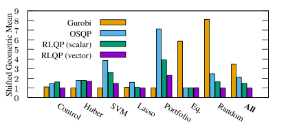
In Fig. 2, we compare the shifted geometric mean of solving 10 problems of 20 different dimension, for a total of 200 runs per class per solver. The problem dimensions for Control, Huber, SVM, Lasso are (10, 11, 12, 13, 14, 16, 17, 20, 23, 26, 31, 37, 45, 55, 68, 84, 105, 132, 166, 209); for Random and Eq are (10, 11, 12, 13, 15, 18, 23, 29, 39, 53, 73, 103, 146, 211, 304, 442, 644, 940, 1373, 2009), and for Portfolio are (5, 6, 7, 8, 9, 10, 12, 14, 16, 20, 24, 28, 35, 43, 52, 65, 80, 99, 124, 154). From the results, we observe that both RLQP adaptation policies typically improve upon convergence rate from the handcrafted policy in OSQP, and in some cases, e.g. Portfolio optimization, by up to 3x.

5.2 Problem Dimension Scaling

Figure 3: Solve time with increasing dimension on the Random QP problem set. We train and benchmark two vector RL adaptation policies: (dashed) on problems ranging from dimension 10 to 50, and (solid) on problems ranging from 10 to 2000. The gray box shows the range of the training data for the dashed line. When the benchmark run is in the same problem-dimension distribution as the training data, the relative performance between solvers is consistent, however, when the problem dimension is outside of he training distribution, the performance diverges.

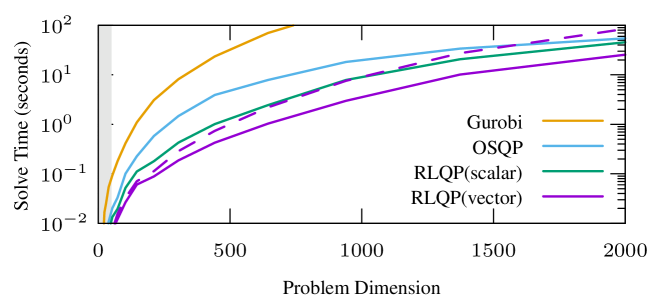
To test how a trained policy scales to higher dimensions, we train a policy on low dimensional problems (10 to 50), and solve problems with varying dimensions, including dimensions higher than the training set (up to 2000). For comparison, we also include a policy trained on the full dimension range (10 to 2000). From the results plotted in Fig. 3, we observe that a policy trained on a lower dimensional training set, can show improvement beyond its training range. However, as the problem size diverges more from the training set, its performance suffers and it eventually loses to the handcrafted policy. Both low-dimensional and full-dimension range polices, were trained using the same network architecture, we hypothesize that this behavior is a function of the training data and not a limitation of the network expressiveness. While this is a disadvantage of using smaller problems for training, in practice it may be outweighed by the advantage in training time—as each RL step requires $O((n+m)^{3})$ compute time.

5.3 Training a Class-Specific Policy

Many applications in control [26] and optimization [27] require QPs from the same class to be repeatedly solved. To test if training a policy specific to a QP class can outperform a policy trained on the benchmark suite, we train policies specific to the problems generated by the trust-region [8] based solver for sequential quadratic program (SQP) from a grasp-optimized motion planner (GOMP) [26, 25] for robots. With these problems, RLQP trained on the benchmarks converges more slowly than the handcrafted policy included in OSQP. With a vector policy trained on the the QPs from the SQP, the shifted geometric mean of OSQP is 1.37. This result suggests that while a general policy may work for multiple problem classes, there are cases in which it is beneficial to train a policy specific to a problem class, particularly if the QPs from that problem class are repeatedly solved.

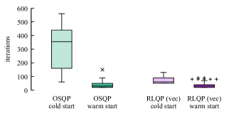
5.4 Warm Starting QPs

One benefit of first-order method such as OSQP is their ability to warm start—that is, rapidly converge from a good initial guess. We test if RLQP retains the benefit of warm start on OSQP’s warm-start benchmark and show the results in Fig. 2 (right). As warm starts require fewer iterations, and thus fewer adaptations than cold starts, we expect RLQP to show a smaller improvement here. In the plot, we can see that RLQP retains the benefit of warm starting, and also gains a improvement over OSQP.

5.5 QPLIB

We benchmark convex continuous QP instances with constraints from QPLIB [15], and show the results in Table 1. Since there are only a few such QPLIB instances and they come from varying classes, creating a train/test split is problematic. We thus use the general policy trained on the benchmark classes. From the table, we observe that the general RLQP policy beats OSQP’s heuristic policy in all but three cases. In two cases RLQP fails due to reaching an iteration or time limit. Training on similar problems should help avoid a timeout.

			non-		RLQP	RLQP
Inst.	$n$	$m$	zeros	OSQP	(scalar)	(vector)
8845	1546	777	10999	6.386	timeout	5.435
9002	2890	1649	12580	6.000	timeout	timeout
8906	5223	838	20781	1.108	1.447	0.741
8559	10000	5000	24998	59.648	205.372	24.083
8938	4001	11999	31997	timeout	timeout	0.991
8567	10000	7500	32497	98.511	284.112	22.222
8616	13870	10404	41610	0.126	0.113	0.141
8515	16002	8002	. 56005	0.105	timeout	timeout
8785	10399	11362	63023	6.334	timeout	2.972
8495	27543	8000	73029	1.612	0.742	1.174
8602	34552	52983	242887	99.872	timeout	55.629
8547	1003001	1001000	6003001	timeout	timeout	timeout

Table 1: QPLIB problems. Timing results for solving the convex continuous QPs with constraints from QPLIB [15]. The Inst. column is QPLIB’s instance number. The columns $n$ (number of variables), $m$ (number of constraints), and non-zeros indicate the QP’s complexity. A timeout result indicates the solver terminated due to reaching an iteration or time limit (300 s). We hypothesize that the RLQP timeouts are due to out of distribution test problems, as the policy here was trained on the benchmark classes.

5.6 Netlib Linear Programming benchmark

The Netlib Linear Programming benchmark [17] contains 98 challenging real-world problems including supply-chain optimization, scheduling and control problems. As with the QPLIB benchmark, we evaluate results with a general policy trained on the benchmark classes. We solve problems to high-accuracy as many of these benchmarks are poorly scaled. Overall, vector formulation of RLQP is 1.30$\times$ faster than OSQP by the scaled geomean of runtimes. We include a problem-specific breakdown in the supplementary materials.

5.7 Maros and Mészáros

In a manner similar to the QPLIB problems, we also benchmark on the Maros and Mészáros repository of QPs. [33]. This collection of 138 QP problems, includes many poorly scaled problems that cause OSQP to fail to converge. We compute the shifted geometric mean for problems solved by both OSQP and RLQP with the general vector policy. RLQP converges faster, with OSQP’s shifted geometric mean is 1.829 times that of RLQP. Because the dataset contains 138 problems, a table of the full results is included in the Supplementary Material.

6 Limitations

RLQP has limitations. For QPs that converge after few iterations, and thus do not adapt $\rho$, having a better adaptation policy is moot. Training RLQP can take a prohibitively long time and require a large replay buffer for some applications, for example, to train the benchmark suite of QPs required several days on a high-end computer with 256 GiB—this may be mitigated to an extent by sharing learned policies between interested practitioners. The time it takes to evaluate the RL policy, especially the vector version, may reduce the performance benefit of faster convergence—this may be mitigated by learning more efficient representations, or by using dedicated neural-network processing hardware.

7 Conclusion

We presented RLQP, a method for using reinforcement learning (RL) to speed up the convergence rate of a first-order method quadratic program solver. RLQP uses RL to learn a policy to adapt the internal parameters of the solver to allow for fewer iterations and faster convergence. In experiments, we trained a generic policy and results suggest that a single policy can improve convergence rates for a broad class of problems. Results for a problem-specific policy suggest that fine-tuning can further accelerate convergence rates.

In future work, we will explore whether additional RL policy options can speed up convergence rate further, such as training a hierarchical policy [2] in which the higher-level policy determines the interval between adaptation, performing a neural-architecture search [11], using meta-learning [13, 39] to speed up problem-specific training, and online-learning to adjust the policy at runtime to adapt to changing problems.

Appendix A Implementation

Training the scalar policy for OSQP [46] requires no modification of the OSQP source code. Instead, we disable the builtin adaptive_rho setting and set max_iter and check_termination to the interval to associate with the policy (e.g., 100). With these settings, the solver will run for the preset iteration count and either return “solved” or “iteration limit reached.” Upon reaching the iteration limit, the RL policy step applies the adaptation via an existing call. On the subsequent step, the internal state of the QP solver remains otherwise unchanged, thus this process mimics adapting the $\rho$ in the inner loop of he solver.

Training the vector policy requires a minor modification of OSQP to support setting and getting the internal $\rho$ vector. Otherwise, training the vector policy is the same as training the scalar policy.

Using and benchmarking the policy requires additional modification of the solver. We modify the code so that when the adaptive_rho setting is enabled, OSQP calls through the PyTorch C++ API [41] to pass the internal state through the learned policy network and then apply the adaptation internally.

We parallelize the training implementation to run multiple episodes concurrently, but otherwise follow close to the TD3 [14] algorithm for the scalar policy, and according to the one-policy [24] modifications described in the main text. When training reaches an update or epoch step, the implementation waits for concurrently running episodes to complete before updating the networks—this leads to imprecise step counts between training, but does not appear to otherwise effect training.

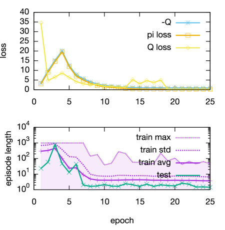
We plot the training curves on learning the benchmark problems in Fig. 4. In this figure we observe that the policy and critic loss lowers over training time, and correspondingly that the episode length (which is the negative reward), goes down as the learned policy improves.

Appendix B Comparison and Ablation of Training and Policies

Figure 4: Reinforcement learning training curves. In these plots, we show the training curves over a training run. The top graph shows the policy (pi) and critic (Q) loss, along with the negated average critic (-Q) value. The bottom graph shows the training episode length maximum (train max), average length + standard deviation (train std), and average length (train avg), and the test episode average. The top graph converges to smaller loss indicating that the policy and critic are improving. The bottom graph shows that average and maximum episode length lowers as training continues.

Figure 5: Comparison of the geometric mean of solve times for policies from different training runs. Here we normalize to the geometric mean of OSQP at 1.0. See text for description of the policies and how they were trained.

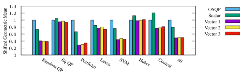
We compare multiple training runs with different seeds for different model architectures, and plot the results in Fig. 5. The Vector 1 policy does not include residuals $\xi_{\mathrm{primal}}$ and $\xi_{\mathrm{dual}}$ in $S$, while Vector 2 and Vector 3 policies do. The Vector 1 and Vector 2 policies are networks with 3 hidden layers, while Vector 3 has 2 hidden layers, all layers are 48 wide with ReLU activations. All policies were trained for a maximum of 50 epochs, with a replay buffer size of $4\times 10^{8}$, $10^{5}$ initial steps, updates every 10000 steps, 5000 batch size, 20000 steps per epoch, 0.995 polyak, 1.0 noise, 2.5 noise clip, and policy updates every other critic update. For 3-layer networks, we set the learning rate to $10^{-5}$ for both policy and critic networks, and for the 2-layer network, we set the learning rate to $10^{-6}$. We selected the epoch with the lowest average loss, though better performance may be possible with a policy from a different epoch. We observe minor variation in the 3 trained policies, but not sufficient to categorically state which one is the best.

Figure 6: Netlib LP performance profiles We evaluate how the learned RLQP policy generalizes to unseen problems. The vector policy is $1.3\times$ faster (shifted geomean) than the existing heuristic in OSQP while solving 5.2% more problems.

Appendix C Netlib Linear Programming Results

In order to measure how well the vector RL policy for OSQP generalizes to unseen inputs, we evaluate the policy on the 98 Netlib LP test problems [17]. These problems are a collection of linear programs considered to be large and challenging. We select this benchmark as this class of linear programs is significantly different than any of the quadratic program classes we train with.

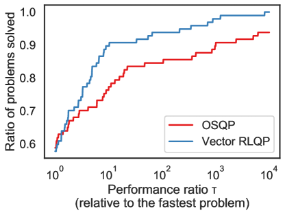
Overall, the vector RLQP policy outperforms the OSQP policy with a shifted geometric mean runtime that is $1.30\times$ faster. Moreover, the vector RLQP policy solves 5.2% more problems than the heuristic OSQP. Figure 6 shows the number of problems solved by OSQP and RLQP with increasing runtime. Performance ratio ($\tau$) represents the rescaled runtime relative to the fastest problem, following the practice of Dolan and Moré [10].

These results are slightly better than the Netlib LP results included in the main paper. With the extra time, we were able to slightly tune the training procedure. Namely, we reduced the replay buffer size (which avoids training the policy with stale rollouts), decreased the learning rate, increased the batch size and finally trained the policy longer. These changes do not substantially change results (from $1.23\times$ to $1.30\times$). Moreover, the Netlib LP problems require a large number of iterations from the OSQP solver. We increased the maximum number of iterations for Netlib LP evaluation to $10^{6}$ iterations.

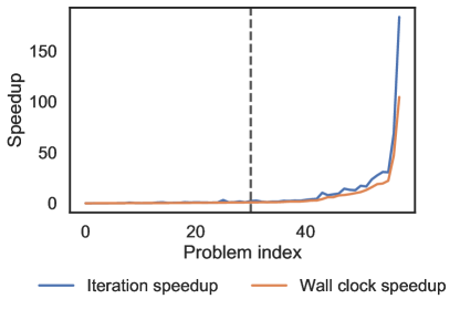
While the vector RLQP policy accelerates Netlib LP optimization overall, it can slow convergence for some problems. In Figure 7 displays per-problem speedups of RLQP over OSQP. RLQP achieves speedups of up to 73x, but degrades performance for a minority of problems. We include detailed per-problem results containing solver runtime in Section E. As we evaluate the policy at fixed intervals, the solver must re-factorize the problem due to a change in $\rho$. However, the policy may update $\rho$ more times than is needed which can slow convergence for some fast well-conditioned problems. Our work is a good starting place for further research into learning methods for first-order optimization. We are extending the RLQP framework to support dynamic policy evaluation which would improve performance for these small-scale problems.

Figure 7: Netlib LP problem speedup Iteration speedup per problem in the Netlib LP problem set. Problems right of the dotted line observe speedup greater than 1. For the majority of problems, RLQP accelerates convergence by up to $73\times$.

Appendix D Maros and Mészáros Results

As with the Netlib linear problems, we evaluate the policy trained on the benchmark problems on all 138 Maros and Mészáros [33] QP problems and present the results here. We have made no effort to ensure that training problems come from the same distribution of QPs as the Maros and Mészáros problems. Many of these QPs are poorly scaled, which causes both OSQP and RLQP to sometimes fail to converge within a 600 s time limit we set. Some problems that OSQP fails to solve, RLQP (vector) solves, and vice versa, while the (scalar) policy performs poorly on most of these problems (not shown). We show results for two (vector) models trained on the benchmarks. The “GNN” model includes the primal and dual residuals ($\xi_{\mathrm{primal}}$ and $\xi_{\mathrm{dual}}$) in $S$, while the “non-GNN” does not. In the table that follows, the bold entries are the fasted solve times in seconds and the fewest ADMM iterations, though we omit the bold when the three policies tie. We report the number of times OSQP and RLQP have the fastest solve time and fewest iterations, and observe that the difference between these indicates that time to compute the adaptation is a factor in making RLQP not outperform OSQP more often.

Appendix E Detailed results for Netlib LP problems

Netlib LP			non-		RLQP
Problem	$n$	$m$	zeros	OSQP	(vector)
25FV47	1876	2697	12581	3.496	31.064
80BAU3B	12061	14323	35325	11.569	52.989
ADLITTLE	138	194	562	0.076	0.079
AFIRO	51	78	153	0.001	0.002
AGG2	758	1274	5498	timeout	1.183
AGG3	758	1274	5514	timeout	0.415
AGG	615	1103	3477	timeout	timeout
BANDM	472	777	2966	0.466	0.264
BEACONFD	295	468	3703	0.025	0.024
BLEND	114	188	636	0.031	0.007
BNL1	1586	2229	7118	timeout	0.998
BNL2	4486	6810	19482	24.329	37.051
BOEING1	726	1077	4553	3.119	0.348
BOEING2	305	471	1663	timeout	0.198
BORE3D	334	567	1782	0.585	0.419
BRANDY	303	523	2505	0.548	0.962
CAPRI	496	767	2461	4.846	0.437
CYCLE	3378	5281	24626	4.931	29.043
CZPROB	3562	4491	14270	10.714	1.388
D2Q06C	5831	8002	38912	127.159	167.348
D6CUBE	6184	6599	43888	3.211	0.321
DEGEN2	757	1201	4958	0.089	0.583
DEGEN3	2604	4107	28036	0.730	3.558
DFL001	12230	18301	47862	14.112	765.502
E226	472	695	3240	0.371	1.126
ETAMACRO	816	1216	3353	0.655	6.718
FFFFF800	1028	1552	7429	timeout	timeout
FINNIS	1064	1561	3824	2.034	2.657
FIT1D	1049	1073	14476	0.390	1.895
FIT1P	1677	2304	11545	0.478	0.080
FIT2D	10524	10549	139566	3.622	119.416
FIT2P	13525	16525	63809	0.533	2.332
FORPLAN	492	653	5126	0.061	0.053
GANGES	1706	3015	8643	4.741	timeout
GFRD-PNC	1160	1776	3605	0.790	0.288
GREENBEA	5598	7990	36668	timeout	timeout
GREENBEB	5602	7994	36677	122.834	timeout
GROW15	645	945	6265	timeout	timeout
GROW22	946	1386	9198	1.132	timeout
GROW7	301	441	2913	timeout	timeout
ISRAEL	316	490	2759	timeout	2.781
KB2	68	111	381	timeout	0.066
LOTFI	366	519	1502	1.599	0.196
MAROS-R7	9408	12544	154256	253.193	timeout
MAROS	1966	2812	12103	timeout	timeout
MODSZK1	1622	2309	4792	1.588	5.152
NESM	3105	3767	16575	0.811	timeout
PEROLD	1594	2219	8911	timeout	timeout
PILOT-JA	2355	3295	18571	timeout	timeout
PILOT-WE	3008	3730	12809	timeout	timeout
PILOT4	1211	1621	8553	timeout	timeout
PILOT87	6680	8710	81629	timeout	timeout
PILOTNOV	2446	3421	15777	timeout	timeout
PILOT	4860	6301	49235	timeout	timeout
QAP12	8856	12048	47160	9.819	26.535
QAP15	22275	28605	117225	91.608	137.196
QAP8	1632	2544	8928	0.386	0.177
RECIPELP	204	295	891	0.002	0.003
SC105	163	268	503	0.011	0.014
SC205	317	522	982	timeout	0.022
SC50A	78	128	238	0.003	0.009
SC50B	78	128	226	0.005	0.023
SCAGR25	671	1142	2396	0.122	timeout
SCAGR7	185	314	650	0.081	0.087
SCFXM1	600	930	3332	2.895	timeout
SCFXM2	1200	1860	6669	timeout	timeout
SCFXM3	1800	2790	10006	15.458	timeout
SCORPION	466	854	2000	timeout	timeout
SCRS8	1275	1765	4563	1.156	7.543
SCSD1	760	837	3148	0.021	0.008
SCSD6	1350	1497	5666	0.262	0.017
SCSD8	2750	3147	11334	0.187	0.031
SCTAP1	660	960	2532	1.492	0.014
SCTAP2	2500	3590	9834	1.094	0.056
SCTAP3	3340	4820	13074	1.192	0.054
SEBA	1036	1551	5396	1.022	0.939
SHARE1B	253	370	1432	1.574	3.544
SHARE2B	162	258	939	timeout	0.030
SHELL	1777	2313	5335	3.615	0.192
SHIP04L	2166	2568	8546	0.716	0.397
SHIP04S	1506	1908	5906	0.091	0.730
SHIP08L	4363	5141	17245	0.372	0.608
SHIP08S	2467	3245	9661	timeout	1.034
SHIP12L	5533	6684	21809	5.992	5.682
SHIP12S	2869	4020	11153	1.081	1.874
SIERRA	2735	3962	10736	5.383	3.165
STAIR	620	976	4641	1.417	timeout
STANDATA	1274	1633	4504	timeout	0.075
STANDGUB	1383	1744	4722	timeout	0.079
STANDMPS	1274	1741	5152	1.329	0.028
STOCFOR1	165	282	666	timeout	0.013
STOCFOR2	3045	5202	12402	2.599	7.081
STOCFOR3	23541	40216	100014	timeout	timeout
TRUSS	8806	9806	36642	10.070	0.770
VTP-BASE	347	545	1399	timeout	2.344
WOOD1P	2595	2839	72811	timeout	0.162
WOODW	8418	9516	45905	9.310	10.675
Total Solved:				67	72

Appendix F Detailed results for Maros & Mészáros problems

				Solve Time			Iteration
Maros & Mészáros			non-		RLQP	RLQP		RLQP	RLQP
Problem	$n$	$m$	zeros	OSQP	non-GNN	GNN	OSQP	non-GNN	GNN
AUG2D	20200	30200	80000	0.155	0.164	0.163	200	200	200
AUG2DC	20200	30200	80400	0.153	0.188	0.155	200	200	200
AUG2DCQP	20200	30200	80400	1.562	23.198	0.939	2200	26800	1000
AUG2DQP	20200	30200	80000	1.683	8.923	0.854	2400	10600	1000
AUG3D	3873	4873	13092	0.028	0.039	0.037	200	200	200
AUG3DC	3873	4873	14292	0.026	0.031	0.035	200	200	200
AUG3DCQP	3873	4873	14292	0.056	0.063	0.065	400	400	400
AUG3DQP	3873	4873	13092	0.053	0.064	0.065	400	400	400
BOYD1	93261	93279	745507	286.552	275.054	timeout	66000	61400	timeout
BOYD2	93263	279794	517049	timeout	timeout	timeout	timeout	timeout	timeout
CONT-050	2597	4998	17199	0.395	0.237	17.030	1600	800	54800
CONT-100	10197	19998	69399	12.062	1.766	timeout	8200	1000	timeout
CONT-101	10197	20295	62496	20.508	3.089	timeout	12800	1800	timeout
CONT-200	40397	79998	278799	352.981	87.121	timeout	33000	7200	timeout
CONT-201	40397	80595	249996	timeout	timeout	timeout	timeout	timeout	timeout
CONT-300	90597	180895	562496	timeout	timeout	timeout	timeout	timeout	timeout
CVXQP1_L	10000	15000	94966	84.758	31.133	104.432	9800	1800	6200
CVXQP1_M	1000	1500	9466	0.161	0.140	0.227	1200	800	1400
CVXQP1_S	100	150	920	0.004	0.003	0.035	800	600	6800
CVXQP2_L	10000	12500	87467	7.049	4.865	4.748	800	400	400
CVXQP2_M	1000	1250	8717	0.046	0.055	0.053	400	400	400
CVXQP2_S	100	125	846	0.001	0.001	0.001	200	200	200
CVXQP3_L	10000	17500	102465	99.156	19.785	23.884	10200	1000	1200
CVXQP3_M	1000	1750	10215	0.795	0.444	40.058	5400	2200	206400
CVXQP3_S	100	175	994	0.002	0.002	0.014	400	400	2200
DPKLO1	133	210	1785	0.002	0.002	0.003	200	200	200
DTOC3	14999	24997	64989	1.389	0.191	7.221	3800	400	16600
DUAL1	85	86	7201	0.002	0.002	0.002	200	200	200
DUAL2	96	97	9112	0.002	0.002	0.003	200	200	200
DUAL3	111	112	12327	0.003	0.003	0.004	200	200	200
DUAL4	75	76	5673	0.001	0.001	0.002	200	200	200
DUALC1	9	224	2025	0.002	0.002	0.002	600	400	400
DUALC2	7	236	1659	0.001	0.002	0.002	400	400	400
DUALC5	8	286	2296	0.001	0.001	0.001	200	200	200
DUALC8	8	511	4096	0.002	0.002	0.003	200	200	200
EXDATA	3000	6001	2260500	4.820	13.794	8.030	2000	3200	2000
GENHS28	10	18	62	0.000	0.000	0.000	200	200	200
GOULDQP2	699	1048	2791	0.020	0.008	0.023	1400	400	1200
GOULDQP3	699	1048	3838	0.003	0.004	0.004	200	200	200
HS118	15	32	69	0.000	0.000	0.000	800	400	400
HS21	2	3	6	0.000	0.000	0.000	200	200	200
HS268	5	10	55	0.000	0.000	0.000	400	400	400
HS35	3	4	13	0.000	0.000	0.000	200	200	200
HS35MOD	3	4	13	0.000	0.000	0.000	200	200	200
HS51	5	8	21	0.000	0.000	0.000	200	200	200
HS52	5	8	21	0.000	0.000	0.000	200	200	200
HS53	5	8	21	0.000	0.000	0.000	200	200	200
HS76	4	7	22	0.000	0.000	0.000	200	200	200
HUES-MOD	10000	10002	40000	0.223	0.174	0.169	1200	800	800
HUESTIS	10000	10002	40000	1.380	0.269	54.088	7600	1200	226600
KSIP	20	1021	19938	0.058	0.025	0.035	1800	600	800
LASER	1002	2002	9462	0.011	0.012	0.014	400	400	400
LISWET1	10002	20002	50004	3.324	278.583	0.851	11200	717600	2400
LISWET10	10002	20002	50004	2.388	0.615	0.312	8200	1600	800
LISWET11	10002	20002	50004	2.441	0.628	0.334	8400	1600	800
LISWET12	10002	20002	50004	2.405	0.684	0.313	8400	1600	800
LISWET2	10002	20002	50004	2.012	0.717	0.283	6800	1800	800
LISWET3	10002	20002	50004	1.935	0.731	0.283	6800	1800	800
LISWET4	10002	20002	50004	2.089	0.635	0.307	6800	1800	800
LISWET5	10002	20002	50004	0.907	0.397	0.212	3200	1000	600
LISWET6	10002	20002	50004	2.417	0.639	0.275	8400	1600	800
LISWET7	10002	20002	50004	2.085	0.885	0.351	7200	2200	1000
LISWET8	10002	20002	50004	2.081	0.791	0.360	7200	2200	1000
LISWET9	10002	20002	50004	2.120	0.787	0.414	7200	2200	1000
LOTSCHD	12	19	72	0.000	0.000	0.000	400	400	400
MOSARQP1	2500	3200	8512	0.028	0.046	0.034	400	600	400
MOSARQP2	900	1500	4820	0.010	0.010	0.011	200	200	200
POWELL20	10000	20000	40000	136.363	283.350	0.796	462400	653200	1200
PRIMAL1	325	410	6464	0.005	0.006	0.006	200	200	200
PRIMAL2	649	745	9339	0.008	0.011	0.008	200	200	200
PRIMAL3	745	856	23036	0.020	0.026	0.021	200	200	200
PRIMAL4	1489	1564	19008	0.019	0.022	0.020	200	200	200
PRIMALC1	230	239	2529	timeout	0.945	0.006	timeout	94400	600
PRIMALC2	231	238	2078	timeout	0.389	0.005	timeout	45800	600
PRIMALC5	287	295	2869	timeout	0.005	0.004	timeout	400	400
PRIMALC8	520	528	5199	timeout	0.435	0.018	timeout	21800	800
Q25FV47	1571	2391	130523	6.124	timeout	8.155	27600	timeout	28200
QADLITTL	97	153	637	0.004	0.004	0.004	1200	1000	1000
QAFIRO	32	59	124	0.000	0.000	0.000	200	200	200
QBANDM	472	777	3023	0.228	0.044	0.049	13600	2000	2200
QBEACONF	262	435	3673	0.032	0.010	0.018	2600	600	1000
QBORE3D	315	548	1872	1.302	0.033	0.368	126200	2600	29000
QBRANDY	249	469	2511	0.170	0.090	0.015	14600	5600	1000
QCAPRI	353	624	3852	2.041	418.003	0.088	146600	22029400	4800
QE226	282	505	4721	0.557	0.147	0.077	36400	7400	3400
QETAMACR	688	1088	11613	0.916	0.140	0.207	10000	1200	1800
QFFFFF80	854	1378	10635	0.362	74.270	15.281	6200	1031600	201400
QFORPLAN	421	582	6112	0.009	timeout	3.255	400	timeout	153200
QGFRDXPN	1092	1708	3739	0.898	0.167	timeout	43400	6600	timeout
QGROW15	645	945	7227	463.025	timeout	0.121	15832000	timeout	3400
QGROW22	946	1386	10837	29.204	timeout	0.116	659400	timeout	2200
QGROW7	301	441	3597	0.536	0.036	timeout	40600	2000	timeout
QISRAEL	142	316	3765	0.043	0.037	0.075	4800	3000	6000
QPCBLEND	83	157	657	0.003	0.003	0.004	1000	600	800
QPCBOEI1	384	735	4253	0.139	0.058	0.056	7000	2200	1800
QPCBOEI2	143	309	1482	0.908	0.022	0.028	148000	2200	3200
QPCSTAIR	467	823	4790	0.086	29.648	0.122	3400	965200	3800
QPILOTNO	2172	3147	16105	60.362	timeout	timeout	411200	timeout	timeout
QPTEST	2	4	10	0.000	0.000	0.000	200	200	200
QRECIPE	180	271	923	0.003	0.004	0.004	600	600	600
QSC205	203	408	785	0.001	0.002	0.001	200	200	200
QSCAGR25	500	971	2282	0.102	timeout	0.154	8800	timeout	9000
QSCAGR7	140	269	602	0.036	0.435	0.005	11200	86400	1000
QSCFXM1	457	787	4456	0.278	131.058	0.872	16400	5741800	41000
QSCFXM2	914	1574	8285	1.160	timeout	11.558	32200	timeout	256600
QSCFXM3	1371	2361	11501	1.698	timeout	2.708	30200	timeout	40200
QSCORPIO	358	746	1842	timeout	0.505	0.237	timeout	40000	19400
QSCRS8	1169	1659	4560	0.508	0.084	0.069	18200	2400	2000
QSCSD1	760	837	4584	0.023	0.017	0.013	1400	800	600
QSCSD6	1350	1497	8378	0.482	0.035	0.031	16400	1000	800
QSCSD8	2750	3147	16214	0.072	0.062	0.049	1200	800	600
QSCTAP1	480	780	2442	timeout	0.016	0.117	timeout	1000	7600
QSCTAP2	1880	2970	10007	0.467	0.060	0.047	8000	800	600
QSCTAP3	2480	3960	13262	0.226	0.042	0.057	2800	400	600
QSEBA	1028	1543	6576	0.201	timeout	0.151	9400	timeout	5800
QSHARE1B	225	342	1436	0.205	0.419	0.060	33800	48400	6800
QSHARE2B	79	175	873	0.117	1.074	0.010	36600	210800	2000
QSHELL	1775	2311	74506	0.328	0.706	6.876	2600	4800	41200
QSHIP04L	2118	2520	8548	0.071	0.059	0.031	1800	1200	600
QSHIP04S	1458	1860	5908	0.039	0.028	0.024	1400	800	600
QSHIP08L	4283	5061	86075	0.192	0.326	0.253	600	800	600
QSHIP08S	2387	3165	32317	0.232	0.093	0.080	2400	800	600
QSHIP12L	5427	6578	144030	1.001	0.525	0.404	2000	800	600
QSHIP12S	2763	3914	44705	0.186	0.056	0.093	1600	400	600
QSIERRA	2036	3263	9582	0.115	0.179	0.351	2000	2400	4800
QSTAIR	467	823	6293	2.567	317.286	0.303	89000	9359600	8200
QSTANDAT	1075	1434	5576	0.245	timeout	0.022	10800	timeout	800
S268	5	10	55	0.000	0.000	0.000	400	400	400
STADAT1	2001	6000	13998	timeout	0.611	timeout	timeout	7000	timeout
STADAT2	2001	6000	13998	timeout	0.244	10.190	timeout	3000	107800
STADAT3	4001	12000	27998	timeout	1.309	292.029	timeout	7200	1489600
STCQP1	4097	6149	66544	0.052	0.058	0.060	200	200	200
STCQP2	4097	6149	66544	0.092	0.086	0.093	200	200	200
TAME	2	3	8	0.000	0.000	0.000	200	200	200
UBH1	18009	30009	72012	1.106	0.463	0.711	2600	800	1200
VALUES	202	203	7846	0.008	0.006	0.010	800	600	1000
YAO	2002	4002	10004	224.794	7.161	4.181	4164000	111800	68000
ZECEVIC2	2	4	7	0.000	0.000	0.000	200	200	200
Problems solved with fewest iterations:							15	38	50
Problems solved with fastest solve time:				31	35	45
Total solved before timeout:				126	125	127

Table 2: Detailed results for the Maros & Mészáros problems [33].

References

- Balcan et al. [2018] Maria-Florina Balcan, Travis Dick, Tuomas Sandholm, and Ellen Vitercik. Learning to branch. In International conference on machine learning, pages 344–353. PMLR, 2018.
- Barto and Mahadevan [2003] Andrew G Barto and Sridhar Mahadevan. Recent advances in hierarchical reinforcement learning. Discrete event dynamic systems, 13(1):41–77, 2003.
- Battaglia et al. [2018] Peter W Battaglia, Jessica B Hamrick, Victor Bapst, Alvaro Sanchez-Gonzalez, Vinicius Zambaldi, Mateusz Malinowski, Andrea Tacchetti, David Raposo, Adam Santoro, Ryan Faulkner, et al. Relational inductive biases, deep learning, and graph networks. arXiv preprint arXiv:1806.01261, 2018.
- Bengio et al. [2020] Yoshua Bengio, Andrea Lodi, and Antoine Prouvost. Machine learning for combinatorial optimization: a methodological tour d’horizon. European Journal of Operational Research, 2020.
- Bertsimas and Stellato [2020] Dimitris Bertsimas and Bartolomeo Stellato. The voice of optimization. Machine Learning, pages 1–29, 2020.
- Boyd et al. [2011] Stephen Boyd, Neal Parikh, and Eric Chu. Distributed optimization and statistical learning via the alternating direction method of multipliers. Now Publishers Inc, 2011.
- Chen and Tian [2018] Xinyun Chen and Yuandong Tian. Learning to perform local rewriting for combinatorial optimization. arXiv preprint arXiv:1810.00337, 2018.
- Conn et al. [2000] Andrew R Conn, Nicholas IM Gould, and Philippe L Toint. Trust region methods. SIAM, 2000.
- Dai et al. [2017] Hanjun Dai, Elias B Khalil, Yuyu Zhang, Bistra Dilkina, and Le Song. Learning combinatorial optimization algorithms over graphs. arXiv preprint arXiv:1704.01665, 2017.
- Dolan and Moré [2002] Elizabeth D Dolan and Jorge J Moré. Benchmarking optimization software with performance profiles. Mathematical programming, 91(2):201–213, 2002.
- Elsken et al. [2019] Thomas Elsken, Jan Hendrik Metzen, Frank Hutter, et al. Neural architecture search: A survey. J. Mach. Learn. Res., 20(55):1–21, 2019.
- Espeholt et al. [2018] Lasse Espeholt, Hubert Soyer, Remi Munos, Karen Simonyan, Volodymir Mnih, Tom Ward, Yotam Doron, Vlad Firoiu, Tim Harley, Iain Dunning, Shane Legg, and Koray Kavukcuoglu. Impala: Scalable distributed deep-rl with importance weighted actor-learner architectures, 2018.
- Finn et al. [2017] Chelsea Finn, Pieter Abbeel, and Sergey Levine. Model-agnostic meta-learning for fast adaptation of deep networks. In International Conference on Machine Learning, pages 1126–1135. PMLR, 2017.
- Fujimoto et al. [2018] Scott Fujimoto, Herke Hoof, and David Meger. Addressing function approximation error in actor-critic methods. In International Conference on Machine Learning, pages 1587–1596. PMLR, 2018.
- Furini et al. [2018] Fabio Furini et al. QPLIB: A library of quadratic programming instances. Mathematical Programming Computation, 2018. doi: 10.1007/s12532-018-0147-4. URL https://doi.org/10.1007/s12532-018-0147-4.
- Gabay and Mercier [1976] Daniel Gabay and Bertrand Mercier. A dual algorithm for the solution of nonlinear variational problems via finite element approximation. Computers & mathematics with applications, 2(1):17–40, 1976.
- Gay [1985] David M Gay. Electronic mail distribution of linear programming test problems. 1985.
- Giselsson and Boyd [2017] P. Giselsson and S. Boyd. Linear convergence and metric selection for douglas-rachford splitting and ADMM. IEEE Transactions on Automatic Control, 62(2):532–544, 2017. doi: 10.1109/TAC.2016.2564160.
- Glowinski and Marroco [1975] Roland Glowinski and A Marroco. Sur l’approximation, par éléments finis d’ordre un, et la résolution, par pénalisation-dualité d’une classe de problèmes de dirichlet non linéaires. ESAIM: Mathematical Modelling and Numerical Analysis-Modélisation Mathématique et Analyse Numérique, 9(R2):41–76, 1975.
- Gould and Scott [2016] Nicholas Gould and Jennifer Scott. A note on performance profiles for benchmarking software. ACM Transactions on Mathematical Software (TOMS), 43(2):1–5, 2016.
- [21] Gurobi Optimization, LLC. Gurobi optimizer. https://www.gurobi.com/. Accessed: 2021-01-28.
- Haarnoja et al. [2018] Tuomas Haarnoja, Aurick Zhou, Pieter Abbeel, and Sergey Levine. Soft actor-critic: Off-policy maximum entropy deep reinforcement learning with a stochastic actor, 2018.
- He et al. [2000] B. S. He, H. Yang, and S. L. Wang. Alternating Direction Method with Self-Adaptive Penalty Parameters for Monotone Variational Inequalities. Journal of Optimization Theory and Applications, 106(2):337–356, August 2000. ISSN 1573-2878. doi: 10.1023/A:1004603514434. URL https://doi.org/10.1023/A:1004603514434.
- Huang et al. [2020] Wenlong Huang, Igor Mordatch, and Deepak Pathak. One policy to control them all: Shared modular policies for agent-agnostic control. In International Conference on Machine Learning, pages 4455–4464. PMLR, 2020.
- Ichnowski et al. [2020a] Jeffrey Ichnowski, Yahav Avigal, Vishal Satish, and Ken Goldberg. Deep learning can accelerate grasp-optimized motion planning. Science Robotics, 5(48), 2020a.
- Ichnowski et al. [2020b] Jeffrey Ichnowski, Michael Danielczuk, Jingyi Xu, Vishal Satish, and Ken Goldberg. GOMP: Grasp-optimized motion planning for bin picking. In 2020 IEEE International Conference on Robotics and Automation (ICRA). IEEE, 2020b.
- Jain et al. [2020] Paras Jain, Ajay Jain, Aniruddha Nrusimha, Amir Gholami, Pieter Abbeel, Joseph Gonzalez, Kurt Keutzer, and Ion Stoica. Checkmate: Breaking the memory wall with optimal tensor rematerialization. In Proceedings of Machine Learning and Systems 2020, pages 497–511. 2020.
- Khalil et al. [2016] Elias Khalil, Pierre Le Bodic, Le Song, George Nemhauser, and Bistra Dilkina. Learning to branch in mixed integer programming. In Proceedings of the AAAI Conference on Artificial Intelligence, volume 30, 2016.
- Li and Malik [2016] Ke Li and Jitendra Malik. Learning to optimize. arXiv preprint arXiv:1606.01885, 2016.
- Lillicrap et al. [2015] Timothy P Lillicrap, Jonathan J Hunt, Alexander Pritzel, Nicolas Heess, Tom Erez, Yuval Tassa, David Silver, and Daan Wierstra. Continuous control with deep reinforcement learning. arXiv preprint arXiv:1509.02971, 2015.
- Littman [1994] Michael L Littman. Markov games as a framework for multi-agent reinforcement learning. In Machine learning proceedings 1994, pages 157–163. Elsevier, 1994.
- Lowe et al. [2017] Ryan Lowe, Yi Wu, Aviv Tamar, Jean Harb, Pieter Abbeel, and Igor Mordatch. Multi-agent actor-critic for mixed cooperative-competitive environments. arXiv preprint arXiv:1706.02275, 2017.
- Maros and Mészáros [1999] Istvan Maros and Csaba Mészáros. A repository of convex quadratic programming problems. Optimization Methods and Software, 11(1-4):671–681, 1999.
- Mattingley and Boyd [2012] Jacob Mattingley and Stephen Boyd. Cvxgen: A code generator for embedded convex optimization. Optimization and Engineering, 13(1):1–27, 2012.
- Metz et al. [2019] Luke Metz, Niru Maheswaranathan, Jeremy Nixon, Daniel Freeman, and Jascha Sohl-Dickstein. Understanding and correcting pathologies in the training of learned optimizers. In International Conference on Machine Learning, pages 4556–4565. PMLR, 2019.
- Mnih et al. [2013] Volodymyr Mnih, Koray Kavukcuoglu, David Silver, Alex Graves, Ioannis Antonoglou, Daan Wierstra, and Martin Riedmiller. Playing atari with deep reinforcement learning, 2013.
- [37] MOSEK ApS. Mosek optimization toolbox. https://www.mosek.com/. Accessed: 2021-01-28.
- Nesterov and Nemirovskii [1994] Yurii Nesterov and Arkadii Nemirovskii. Interior-point polynomial algorithms in convex programming. SIAM, 1994.
- Nichol et al. [2018] Alex Nichol, Joshua Achiam, and John Schulman. On first-order meta-learning algorithms. arXiv preprint arXiv:1803.02999, 2018.
- Nocedal and Wright [2006] Jorge Nocedal and Stephen Wright. Numerical optimization. Springer Science & Business Media, 2006.
- Paszke et al. [2019] Adam Paszke et al. PyTorch: An imperative style, high-performance deep learning library. In H. Wallach, H. Larochelle, A. Beygelzimer, F. d'Alché-Buc, E. Fox, and R. Garnett, editors, Advances in Neural Information Processing Systems 32. 2019.
- Scarselli et al. [2008] Franco Scarselli, Marco Gori, Ah Chung Tsoi, Markus Hagenbuchner, and Gabriele Monfardini. The graph neural network model. IEEE transactions on neural networks, 20(1):61–80, 2008.
- Schulman et al. [2013] John Schulman, Jonathan Ho, Alex X Lee, Ibrahim Awwal, Henry Bradlow, and Pieter Abbeel. Finding locally optimal, collision-free trajectories with sequential convex optimization. In Robotics: science and systems, volume 9, pages 1–10. Citeseer, 2013.
- Schulman et al. [2017] John Schulman, Filip Wolski, Prafulla Dhariwal, Alec Radford, and Oleg Klimov. Proximal policy optimization algorithms, 2017.
- Silver et al. [2014] David Silver, Guy Lever, Nicolas Heess, Thomas Degris, Daan Wierstra, and Martin Riedmiller. Deterministic policy gradient algorithms. In International conference on machine learning, pages 387–395. PMLR, 2014.
- Stellato et al. [2020] B. Stellato, G. Banjac, P. Goulart, A. Bemporad, and S. Boyd. OSQP: an operator splitting solver for quadratic programs. Mathematical Programming Computation, 12(4):637–672, 2020. doi: 10.1007/s12532-020-00179-2. URL https://doi.org/10.1007/s12532-020-00179-2.
- Sutton et al. [1999] Richard S Sutton, David A McAllester, Satinder P Singh, Yishay Mansour, et al. Policy gradient methods for reinforcement learning with function approximation. In NIPs, volume 99, pages 1057–1063. Citeseer, 1999.
- Wei et al. [2020] Kaixuan Wei, Angelica Aviles-Rivero, Jingwei Liang, Ying Fu, Carola-Bibiane Schönlieb, and Hua Huang. Tuning-free plug-and-play proximal algorithm for inverse imaging problems. In International Conference on Machine Learning, pages 10158–10169. PMLR, 2020.
- Wolfe [1959] Philip Wolfe. The simplex method for quadratic programming. Econometrica: Journal of the Econometric Society, pages 382–398, 1959.