Spin-orbit effects for compact binaries in scalar-tensor gravity
Abstract
Gravitational waves provide us with a new window into our Universe, and have already been used to place strong constrains on the existence of light scalar fields, which are a common feature in many alternative theories of gravity. However, spin effects are still relatively unexplored in this context. In this work, we construct an effective point-particle action for a generic spinning body that can couple both conformally and disformally to a real scalar field, and we show that requiring the existence of a self-consistent solution automatically implies that if a scalar couples to the mass of a body, then it must also couple to its spin. We then use well-established effective field theory techniques to conduct a comprehensive study of spin-orbit effects in binary systems to leading order in the post-Newtonian (PN) expansion. Focusing on quasicircular nonprecessing binaries for simplicity, we systematically compute all key quantities, including the conservative potential, the orbital binding energy, the radiated power, and the gravitational-wave phase. We show that depending on how strongly each member of the binary couples to the scalar, the spin-orbit effects that are due to a conformal coupling first enter into the phase at either 0.5PN or 1.5PN order, while those that arise from a disformal coupling start at either 3.5PN or 4.5PN order. This suppression by additional PN orders notwithstanding, we find that the disformal spin-orbit terms can actually dominate over their conformal counterparts due to an enhancement by a large prefactor. Accordingly, our results suggest that upcoming gravitational-wave detectors could be sensitive to disformal spin-orbit effects in double neutron star binaries if at least one of the two bodies is sufficiently scalarised.
1 Introduction
The successful detection of gravitational waves is a triumph of our time. Observations by the LIGO Scientific and Virgo collaborations continue to fall into excellent agreement with the predictions of general relativity [1, 2, 3, 4, 5], and can thus provide powerful constraints on any departure from Einstein’s theory. However, fully exploiting this new window into our Universe requires that we develop a more complete understanding of how deviations from general relativity can arise. In this work, we take another step forward in this direction by studying how a real scalar field can couple to both the mass and the spin of a compact object. We compute (for the first time) the effect of such a coupling on the phase of the outgoing gravitational-wave signal from a compact binary; thereby providing a novel means with which to search for the imprints of hidden scalar degrees of freedom.
There are many reasons why one might think to augment general relativity in this way. On the one hand, light scalar fields lie at the heart of much cosmological model building [6, 7, 8, 9, 10, 11]; motivated primarily by the difficulty in otherwise accounting for the observed, late-time acceleration of our Universe [12, 13]. This is the well-known cosmological constant problem [14]. Indeed, because general relativity is only an effective description of gravity at low energies — requiring as-of-yet unknown new physics to become important at the Planck scale, if not before — the act of including additional, light degrees of freedom in the effective field theory allows us to capture a greater range of possible effects that could stem from new fundamental physics. Since the simplest way of going beyond the tensor modes of general relativity is to add a single scalar field, scalar-tensor theories have become the main workhorse for building and testing alternative models of late-time cosmology, where the scalar plays the role of dark energy [15, 16, 17, 18, 19, 20, 21, 22, 23, 24], or even dark matter [25, 26, 27, 28, 29, 30, 31, 32, 33]. On smaller scales, scalar-tensor theories are also widely used to effect deviations from general relativity in the strong-field regime [34, 35, 36, 37, 38, 39, 40, 41, 42, 43, 44, 45, 46, 47, 48, 49, 50, 51, 52, 53, 54, 55, 56, 57, 58, 59, 60, 61, 62, 63, 64, 65, 66, 67, 68, 69, 70, 71].
By virtue of their interesting phenomenology, the existence of light scalar fields and how they couple to gravity and/or matter have been the subject of extensive study. On theoretical grounds, the most general, causality-preserving coupling between a scalar and matter with energy-momentum tensor is composed of two parts: a conformal part and a disformal part [72]. The conformal part of the coupling, which has the schematic form , is already tightly constrained in the Solar System by measurements from the Cassini spacecraft [73] and lunar laser ranging [74]. The implications of this kind of interaction have also been confronted with experiments in the laboratory [75, 76, 77, 78, 79], in other astrophysical settings [80, 81, 82, 83, 84, 85, 86, 41, 42, 43], and on cosmological scales [87, 88, 89]. (See also refs. [90, 91, 92] for general reviews.) The disformal part of the coupling, meanwhile, is more challenging to constrain in nonrelativistic settings, as its general form inevitably results in a suppression by the relevant velocity scale in the problem, and so causes it to vanish around static sources. Nevertheless, constraining this interaction is important, as it arises naturally in a variety of scenarios, including (beyond) Horndeski and general DHOST theories [93, 94, 95, 96, 97, 98, 99, 100, 101, 102, 103, 104], in the decoupling limit of massive gravity [105, 106, 107], in branon models [108, 109], and in various brane-world scenarios [110, 111]. Moreover, a disformal interaction often appears at a much lower energy scale than its conformal counterpart (i.e., ), thus making it a (potentially) very powerful probe of the dark sector. Our goal in this work is to complement existing laboratory and astrophysical searches for disformal couplings [112, 113, 114, 115, 116, 117, 118, 119, 120, 121, 122, 123, 124, 125, 126, 127, 128] by examining the impact of such an interaction on the gravitational waves emitted by a compact binary.
As we enter this age of gravitational-wave astronomy, binary systems are fast becoming one of the most promising probes of light scalar fields. Arguably the most striking example to date is the neutron-star merger event GW170817 [129, 130, 131, 132], whose optical counterpart suggests that photons and gravitational waves travel at the same speed to within one part in (at least, at LIGO/Virgo frequencies111Since the speed of gravitational waves, like any coupling in a quantum field theory, depends on the scale at which it is measured, care must be taken when applying this constraint to effective field theories whose cutoff is close to LIGO/Virgo scales ( Hz), as is often the case for dark energy [133].); leading to very stringent constraints on certain scalar-tensor theories [134, 135, 136, 137, 138, 139, 140, 141, 142]. Propagation effects aside, a light scalar field will also influence the orbital motion of the binary itself, and thereby leave imprints in the precise shape and phase of the gravitational waveform that is produced [143, 144, 145, 146, 147, 148, 149, 150, 151]. Decoding these imprints is theoretically challenging, but is nevertheless important because it probes the dark sector in a unique regime; far away from what is possible on laboratory, Solar System, and cosmological scales.
To date, the majority of work on the two-body problem in scalar-tensor gravity has focused on nonspinning systems, with relatively little attention paid to the effect that a scalar would have on a spinning body. Perhaps the main reason for this is that, up until very recently, black holes were thought incapable of coupling to scalars on account of the no-hair theorems [152, 153, 154, 155, 156, 157, 158, 159, 160, 161, 162], while neutron stars (and other bodies composed of matter) are generally expected to spin too slowly for a spin-dependent coupling to leave significant imprints on the gravitational-wave signal [163]. Today we know that black holes can indeed couple to a scalar field — either indirectly through the effect of a time-dependent background [164, 165, 166, 167, 168, 169, 170, 171, 172], or directly via a coupling to a quadratic curvature invariant like the Gauss-Bonnet term [45, 46, 47, 48, 49, 50, 51, 52, 53, 54, 37, 55, 56, 57, 58, 59].222While we focus on real scalar fields in this work, it is worth noting that massive, complex scalars [173, 174] and pseudoscalars [175, 176, 177] can also produce black hole solutions that circumvent the no-hair theorems. Binary black holes that couple to the latter are studied in refs. [178, 179, 180]. Characterising how a scalar interacts with the spins of these “hairy” black holes will undoubtedly give us a better understanding of their behaviour in a binary system, and could be important for establishing more accurate constraints on this class of models. As for neutron stars, these objects are still expected to have much smaller spins than their black hole cousins, and while it remains unlikely that a conformal spin-dependent coupling would leave a significant imprint on the gravitational waveform, it is conceivable that a sufficiently small value of could be enough to boost the size of the disformal coupling between the scalar and the spin of the neutron star to a detectable level. This spin-dependent interaction will be especially important when searching for disformally coupled scalar fields in (nearly) circular binaries, like those observed by LIGO and Virgo, as the spin-independent effects associated with a disformal coupling are known to vanish for circular orbits [181, 182].
With all of this in mind, the central aim of this paper is to compute the leading spin-orbit effects that would arise when a compact binary is coupled both conformally and disformally to a light scalar field. We focus here on the early portion of the binary’s inspiral, which is amenable to analytic methods, and will use a generalisation of the “nonrelativistic general relativity” (NRGR) approach [183, 184, 185, 186, 187, 188, 189, 190, 191, 192, 193, 194, 195, 196] to perform our calculations. When read alongside existing spin-independent results [197, 198, 199, 200, 201, 202, 203, 204, 205, 181, 182], the spin-orbit results of this paper offer a more complete picture of how these systems behave in scalar-tensor gravity.
It is worth noting at this stage that some partial spin-orbit results have already been derived in a previous paper of ours [206], albeit with two key limitations. The first is that ref. [206] was restricted to a purely conservative setting, whereas the results of this paper go as far as to also include the leading spin-orbit effects from a scalar in the radiative sector. The second limitation of ref. [206] is that it applies only to weakly gravitating bodies that are universally coupled to the scalar, and so satisfy the weak equivalence principle. In contrast, the results of this paper remain valid also for strongly gravitating bodies, like black holes and neutron stars, which emphatically do not respect the strong equivalence principle [207], even if the underlying scalar-tensor theory respects the weak equivalence principle at a microscopic level. Both of these advancements were made possible by our use of the NRGR approach, which allows us to work efficiently at the level of the action, rather than laboriously at the level of the equations of motion (as we did in ref. [206]).
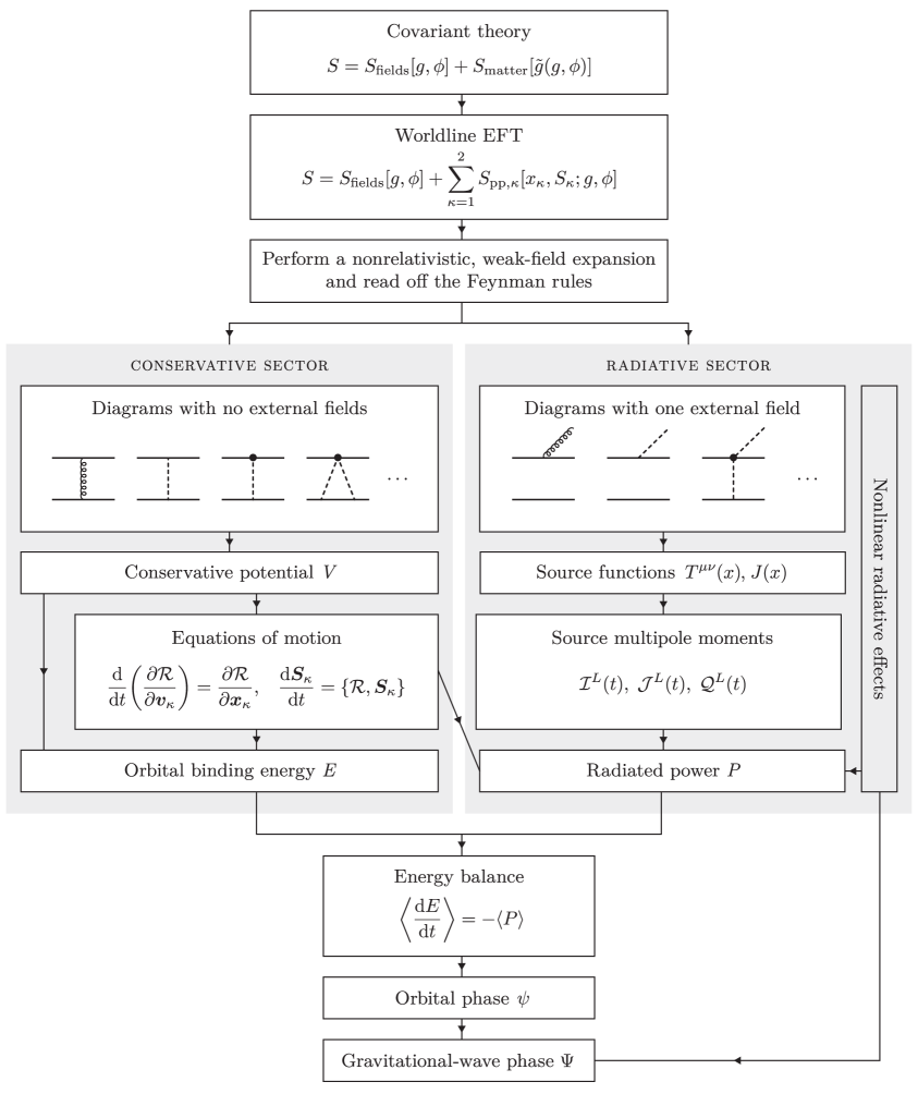
The main conceptual ideas that underpin this NRGR approach are reviewed in section 2, where we also review the general pipeline that takes us from a fully covariant, microscopic theory of fields to an effective field theory for the compact binary — wherein the two extended bodies are replaced by point-particle sources — and ultimately to a concrete prediction for the gravitational-wave phase (see also figure 1). We then work through this sequence of steps in explicit detail across sections 3–5. In section 3, we begin by constructing a general point-particle action for a single spinning body that is conformally and disformally coupled to the scalar field. The most salient details about the body’s internal structure are encoded in this action through the values of Wilson coefficients, and while it is possible to match this point-particle action back onto the underlying, microscopic theory to determine what values these coefficients must take to coincide with a particular object (see section 3.2 for details), we will leave these Wilson coefficients as free parameters in this work; thereby keeping our results general enough to describe the behaviour of any spinning body.
In section 4, we turn to consider a binary system of two such objects. We use Feynman diagrams to compute the spin-orbit part of the conservative two-body potential; working perturbatively to leading order in the post-Newtonian expansion and up to first order in the disformal coupling. For added simplicity, we also assume throughout this paper that any nonlinear self-interactions of the scalar are subleading on the scales of the binary, and can therefore be neglected as a first approximation. This is a valid simplification even for theories that exhibit thin-shell screening [208, 209, 210, 211, 212, 213, 214],333In these models, nonlinearities become important only in the high-density interiors of the two bodies; hence, the primary effect of thin-shell screening can be captured by simply matching the right values for the bodies’ Wilson coefficients. See refs. [213, 214] for more details. although models that utilise derivative self-interactions to trigger kinetic or Vainshtein screening [215, 94, 216, 217, 218] are notably outside the purview of our results. (See, e.g., refs. [219, 220, 221, 222, 223, 224] for spin-independent progress in this direction.) To complete our discussion of the binary’s conservative sector, we then derive the corresponding equations of motion for this system and identify some of its constants of motion; the most important of which being its orbital binding energy.
In section 5, we move on to the radiative sector, where we use similar diagrammatic techniques to compute the multipole moments responsible for sourcing the outgoing scalar and gravitational waves. Focusing on quasicircular nonprecessing binaries for simplicity, we then combine our result for the total radiated power with our earlier expression for the orbital binding energy to determine the evolution of the binary’s orbital phase, and by extension, its gravitational-wave phase. These general results establish what the leading spin-orbit effects would be in any kind of binary system, but for the sake of having a concrete example, we specialise to double neutron stars in section 6, where we provide estimates for the typical size of these effects. We then argue that a future ground-based detector, like the Einstein Telescope, could be capable of observing the imprints of a disformal spin-orbit interaction if at least one of the neutron stars is sufficiently scalarised. Finally, in section 7, we conclude with a summary of our main results and identify several key directions for future work.
2 The effective field theory pipeline
The decisive property that allows us to make analytic predictions about how compact binaries evolve is the presence of large separations of scales that are inherent during the early inspiral. In the NRGR approach [183, 184, 185, 186, 187, 188, 189, 190, 191, 192, 193, 194, 195, 196], these separations of scales are used to establish a tower of effective field theories (EFTs) that — when matched onto another — provide a coherent description of the system and facilitate the systematic computation of observables, like the phase of the emitted gravitational-wave signal. It is this approach, suitably generalised to scalar-tensor theories, that we shall adopt in this paper.
Our goal in this section is to first outline the general sequence of steps that will take us from a given scalar-tensor theory to a concrete result for the gravitational-wave phase; the intention being that having this overview to refer to will help guide our discussion when it comes time to wade through numerous and lengthy calculations. To complement the main text, an illustrated version of this review is also presented in figure 1.
Scalar-tensor theories.
Our very first step, then, is to be precise about the class of scalar-tensor theories under consideration. We will here be interested specifically in metric theories of gravity that can be captured by the general action
| (2.1) |
The kinetic terms for and the interactions between the Einstein-frame metric and the scalar field are contained in the field action , while the dynamics of the matter fields and their couplings to and are encoded in the matter action . Crucially, what makes this a metric theory of gravity is our assumption that the matter fields are coupled minimally and universally to an effective Jordan-frame metric , which we take to be [72]
| (2.2) |
Notice that the conformal coupling function is dimensionless by construction, and so must depend on and only via the dimensionless combinations and , where is the reduced Planck mass and is some strong-coupling scale.444In cosmological applications, one typically sets equal to the Hubble constant so as to produce order-one deviations from general relativity on these scales, but for our purposes it will be more instructive to leave as a free parameter to be constrained by gravitational-wave observations. For simplicity, we will suppose that the disformal coupling function also depends on only through these same combinations and , and that this dimensionful function has an overall scaling of the form .
This kind of scaling automatically tells us that the theory in (2.1) is nonrenormalisable, and so must be viewed as a low-energy EFT of some as-of-yet unknown UV completion. That said, for appropriate choices of the model parameters, this fully covariant EFT can still be valid down to microscopic scales, and so presently encodes more information than is necessary for describing the evolution of astrophysical systems.
Point-particle approximation.
When modelling the inspiral of a (widely separated) two-body system, this surplus of irrelevant information is discarded by replacing (2.1) with the effective action
| (2.3) |
which is valid on length scales greater than the individual radii of the binary’s constituents. In this regime, the two extended bodies (labelled by ) have been replaced by effective point particles whose centres of energy travel along the worldlines . The details about how these point particles move in the bulk of the spacetime and how they interact with the metric and scalar are encoded in the point-particle actions , while the dynamics of the bulk fields continue to be captured by the same field action as before.
We may regard this coarse-grained description of the system as emerging directly from (2.1) after having integrated out all of the irrelevant short-wavelength degrees of freedom, although in practice it is much simpler to construct these point-particle actions from the bottom up. In a Lagrangian approach, the relevant objects available for contraction with , , and their derivatives are the particle’s 4-velocity and its angular velocity tensor (see section 3 for details), but it is traditional — and also more convenient — to work with the spin tensor in place of . As this spin tensor is the momentum variable conjugate to , we can pass from one to the other by performing a partial Legendre transform of the Lagrangian to obtain the point-particle Routhian [225, 188, 189].
Having done so, it follows that the action () is composed of an infinite series of terms, which one can order by relevancy, that couple and to the bulk fields. Multiplying most of these terms are Wilson coefficients , whose values encode all of the salient information about the underlying scalar-tensor theory, as well as the internal structure of the extended objects. One can then determine these values by matching appropriate observables computed within this point-particle EFT to results obtained in the full theory (2.1), but we shall make no attempt to do so here and will simply leave these Wilson coefficients as free parameters. The advantage in doing so is that our results will be applicable to a broad class of models.
Potential and radiation modes.
Two more simplifications are necessary to render the problem analytically tractable. We first make the weak-field approximation by writing
| (2.4) |
where the part that is sourced by the binary is to be treated as a weak perturbation about some fixed background . Implicit in this choice of background is the assumption that the binary’s immediate neighbourhood is mostly just empty space, albeit permeated by some ambient value of the scalar that we take to be a constant.555If the scalar is a candidate for dark energy or fuzzy dark matter, this background value will exhibit some mild time dependence, although the large hierarchy between the typical timescales in a binary and those of cosmology mean that any effects resulting from this time-dependent background are usually small [165, 199, 167, 226, 227], and so will be neglected here.
We then split the field perturbations further into different parts based on their kinematics. In pure general relativity, the metric perturbation (or “graviton”) splits into two parts [183]: there are potential modes that are always off shell and are responsible for mediating the attractive forces holding the two-body system together, and there are radiation modes that can go on shell and transport energy and momentum away from the binary. The former varies on length scales on the order of the distance between the two bodies, while the latter varies on length scales , where is the binary’s orbital velocity. If we now suppose that the scalar perturbation is sufficiently light that it is effectively massless on length scales , then it too admits this simple decomposition into potential and radiation modes. We shall make this assumption throughout, and so are justified in writing
| (2.5) |
where denote the potential modes, while are the radiation modes.
That the radiation modes have wavelengths much larger than the characteristic size of the binary during the early inspiral allows us to “zoom out” on this system even further by integrating out the potential modes. The result is a new EFT,
| (2.6) |
whose action can be organised into a conservative and radiative sector:
| (2.7) |
Most of the hard work in the NRGR approach is in the evaluation of (2.6). It goes without saying that, for astrophysical binaries, we are ultimately interested only in the classical limit of this result, but framing the problem in this kind of quantum field theoretic language allows us to use the machinery of Feynman diagrams to our advantage when computing (2.7) systematically to some prescribed order in the post-Newtonian (PN) expansion; i.e., to some order in . For classical processes, only the tree-level Feynman diagrams are needed [183].
Conservative sector.
The conservative sector of (2.7) encodes information about the orbital dynamics of the binary in the absence of any outgoing radiation, and may be written as the integral of the two-body Routhian
| (2.8) |
over the coordinate time (i.e., ). The conservative potential arises from summing over all Feynman diagrams involving internal potential lines only and no external ones:
| (2.9) |
The explicit calculations leading to this potential are discussed further in section 4.
Because the Routhian in (2.8) has been obtained by Legendre transforming the particles’ rotational degrees of freedom, it behaves like a Lagrangian from the point of view of the position variables, but behaves like a Hamiltonian with respect to the spin variables. The equations of motion therefore follow from a mixture of Euler–Lagrange and Hamilton equations; namely,666When working in harmonic coordinates to 2PN order or higher, the conservative potential will also generally depend on the accelerations and their higher time derivatives [228]. However, appropriate field redefinitions can always be made to replace these by functions that depend on and only [229], thus ensuring that satisfies a second-order equation of motion. One also encounters time derivatives of in the potential at sufficiently high PN orders, but in this case, the appropriate field redefinitions cannot be made when working with a Routhian (in fact, the spin equations of motion no longer follow from a Poisson bracket), and so one is compelled to revert back to a Lagrangian of first-order form involving both and [230, 192]. That said, we will only consider spin effects to leading PN order in this paper, for which the Routhian approach will suffice, and will in fact be the most convenient.
| (2.10) |
It is worth highlighting that these equations are expressed in terms of the 3-vectors and , rather than the worldline coordinates and spin tensor that we started with in (2.3). The gauge-fixing procedure that removes the unphysical degrees of freedom in and is discussed in detail in sections 3 and 4.
Radiative sector.
Turning now to the radiative sector, we find that the remaining terms in naturally group themselves into two categories:
| (2.11) |
The first term gives us the propagators for and the interactions between the radiation modes, while the second accounts for how these fields are sourced by the binary. As we discussed previously, the radiation modes vary on length scales much greater than the orbital separation between the two bodies, and so are unable to resolve either of them individually — instead perceiving the entire two-body system as behaving like a single point particle. Mathematically, this notion is reflected in the way the interactions are organised in ; namely, in terms of multipole moments for the binary as a whole.
To go from (2.3) to the multipole moments in (2.11), one proceeds as follows. First, we integrate out the potential modes while holding the radiation modes fixed to determine the source functions and . In the scalar sector, we sum over all Feynman diagrams with one external radiation-mode scalar to obtain
| (2.12) |
from which can be deduced. (Any internal lines in these diagrams correspond to potential modes.) Similarly, the binary’s energy-momentum tensor follows from summing over all Feynman diagrams with one external radiation-mode graviton:
| (2.13) |
Next, we perform a Taylor expansion of the radiation fields about the binary’s centre of energy, which we may take to coincide with the origin of our coordinate system without any loss of generality. Then regrouping terms into symmetric and trace-free (STF) operators, the result in the scalar sector is777We are employing standard multi-index notation: we write to denote any tensor with spatial indices, while any vector repeated times is abbreviated to read , and likewise . Lastly, angled brackets around indices instruct us to keep only the STF part of that tensor.
| (2.14) |
where the binary’s scalar multipole moments are given by [231]
| (2.15) |
Identical steps can then be taken in the gravitational sector to obtain analogous formulae relating to the binary’s mass-type and current-type multipoles, and ; see, e.g., eqs. (7.44) and (7.45) of ref. [195] for the explicit expressions. With these multipole moments in hand, it is then a straightforward exercise to solve the wave equations (as derived from ) for and to determine the rate at which energy is carried off to infinity. Ignoring nonlinear effects like tail terms, the power radiated away into scalar waves is [231]
| (2.16a) | |||
| while the power radiated into gravitational waves is [231, 232] | |||
| (2.16b) | |||
In writing these formulae, we have used the short hand to denote the action of multiple time derivatives, and note also that the angled brackets around the multipoles denote a time average over several orbital periods. These multipole moments, and the corresponding power that is radiated away, are discussed in more detail in section 5.
Phase evolution.
The two key outputs from the above calculations — the binding energy from the conservative sector, which follows from the equations of motion in (2.10), and the total power computed in the radiative sector — can now be combined into the balance equation
| (2.17) |
to tell us how the binary’s orbit evolves as it emits gravitational and scalar waves. For circular nonprecessing orbits, which will be the targets of our focus in this paper, both and depend on time only through the orbital frequency , and so (2.17) can in this case be recast into a differential equation for the binary’s orbital phase .
After solving this equation (a task we undertake towards the end of section 5), all that remains is to relate the orbital phase to the gravitational-wave phase . At the detector, the gravitational-wave signal can be decomposed into spin-weighted spherical harmonics labelled by the familiar integers , and the phase of the mode is simply given by , up to corrections from nonlinear effects like tail terms [233, 203], which we neglect. Any scalar waves that reach the detector can also be decomposed into spherical harmonics, and the corresponding modes will possess the same phases up to nonlinear corrections. However, in viable scalar-tensor theories, for which the strength of the scalar-matter couplings in the weak-field regime are strongly constrained, these scalar waves leave a much smaller imprint on the detector than their gravitational counterparts [144, 143]. It will therefore suffice to focus on just the gravitational-wave signal in what follows.
3 Spinning point particles in scalar-tensor theories
Having reviewed the general EFT pipeline, we are now in a better position to begin undertaking detailed calculations. The aim of this section is to construct a general point-particle action for spinning bodies that are coupled to both a metric and a real scalar .
We do so in three stages. We start off in section 3.1 by first describing the phase space of one such particle, before reviewing the simple arguments that lead to a first-order Lagrangian that minimally couples it to general relativity. This Lagrangian is then generalised to include additional couplings to the scalar in section 3.2. Finally, in section 3.3, we perform the requisite Legendre transformation that turns this Lagrangian into a Routhian, as will be needed in the next step of our EFT pipeline.
3.1 Covariant degrees of freedom
In any generally covariant theory, a spinning point particle can be described by a worldline and an orthonormal tetrad . The first specifies for us the trajectory along which this particle’s centre of energy travels, while the latter may be regarded as the Jacobian for transforming between a general coordinate chart and the particle’s body-fixed frame . This transformation encodes information about the intrinsic rotation of the particle, which proceeds with an angular velocity given by , where is the covariant derivative along the tangent () to the worldline. If we now introduce the conjugate momentum variables
| (3.1) |
we may easily write down the action for this point particle in first-order form:
| (3.2) |
Before we can specify the exact form of the Hamiltonian , a few more words on the phase-space variables are in order. To start with, note that the transformation from a general set of coordinates to the body-fixed coordinates can be effected in two stages: one first performs a rescaling of the metric to go into the locally flat frame, followed by a Lorentz transformation to go into the body-fixed frame. Mathematically, we write , where is the vierbein that takes us into the locally flat frame, while is the appropriate Lorentz transformation. The usefulness of this decomposition is that it separates into a part that depends only on the particle’s translational degrees of freedom (the vierbein ) and a part that depends only on its rotational degrees of freedom (the Lorentz matrix ). Substituting this into our definition of then reveals that
| (3.3) |
where is the angular velocity relative to the locally flat frame (which is emphatically different from ), while is the corresponding spin tensor in this frame. Crucially, because the “kinetic term” for the rotational degrees of freedom is independent of the metric, we see that a minimal coupling between gravity and spin appears solely through an interaction term involving the spin connection
| (3.4) |
Let us now count the total number of degrees of freedom. The generalised coordinates and their conjugate momenta together give us a total of 20 phase-space variables: the worldline coordinates and the linear momentum contain four degrees of freedom each, the Lorentz matrix is constrained by its defining property and so has six degrees of freedom, while the spin tensor is antisymmetric by construction and so carries another six degrees of freedom. This is ultimately eight too many (only 12 phase-space variables, or six generalised coordinates, are needed to uniquely describe a spinning point particle — three coordinates for its position and three angles to describe its orientation); hence, we must impose a commensurate number of constraints. This can be accomplished by choosing [234]
| (3.5) |
where the fields , , and serve as Lagrange multipliers.
Starting from the right, we see that extremising the action with respect to enforces the constraint [235].888We use the “” symbol to denote a weak equality in the sense of Dirac [236]. This constraint, which is known as the covariant spin supplementary condition (SSC), removes the three unphysical degrees of freedom contained in the spin tensor , and removes no more than three because is trivially orthogonal to . Next, extremising with respect to imposes the conjugate constraint [237], which also removes just three degrees of freedom, since is orthogonal to . In physical terms, what this constraint on amounts to is a gauge fixing of the (superfluous) boost degrees of freedom, which thereby sets the timelike vector parallel to the particle’s 4-momentum . The choice of SSC, meanwhile, essentially determines what we mean by the “centre of energy” of this spinning object [238]. We will work exclusively with these gauge choices in what follows, although it is worth mentioning that other choices are certainly possible [238, 187, 192].
Returning to (3.5), we now see that extremising the action with respect to the einbein enforces the mass-shell constraint . Because rotational energy necessarily gravitates, the particle’s Arnowitt-Deser-Misner (ADM) mass is generically a function of the spin’s absolute magnitude; i.e., with [237, 239, 240]. Specifying an exact form for this functional dependence will, however, turn out to be unnecessary. As we show in appendix A, the equations of motion descending from this action guarantee that is conserved; hence, is also a constant of the motion regardless of how it depends on .999See, e.g., ref. [241] for a point-particle action that conserves neither nor . Such an action is useful for incorporating dissipative effects, such as the absorptive nature of a black hole’s horizon.
The reader keeping score should have counted a total of seven independent constraints imposed thus far, which means that there is still one more to go. This last constraint is also enforced by the einbein, albeit more subtly, as its presence renders the action reparametrisation invariant. Said in other words, the transformation and is a gauge symmetry of the point-particle action.101010That the einbein is playing this dual role as both a Lagrange multiplier and a Stueckelberg field is ultimately tied to the fact that, in the Hamiltonian description of this problem, the mass-shell constraint is first class, whereas the spin constraints and are second class [237, 239]. Fixing a gauge for the worldline parameter therefore removes the last remaining unphysical degree of freedom, contained in . For post-Newtonian applications, the most natural gauge choice would be to set (as we do in section 4), while for fully relativistic problems, one might instead prefer to work with the condition , which sets equal to the proper time.
3.2 Scalar couplings and strong-gravity effects
Up to higher-order terms that account for its finite size [183, 187, 192, 243, 244, 245, 246, 247, 248, 241], the action that we have just written down can be used to describe the behaviour of any extended, spinning object in general relativity. Moreover, because the weak equivalence principle holds in the Jordan frame by construction, this same action will also describe how weakly gravitating objects behave in the scalar-tensor theories of (2.1) once we replace by the Jordan-frame metric . (Strongly gravitating objects will be discussed shortly.) To make this manifest, let us affix tildes to everything, such that the Lagrangian in the Jordan frame reads
| (3.6) |
Disformal transformations.
Going back to the Einstein frame by way of (2.2) will now generate direct couplings between this point particle and the scalar . At the level of the vierbeins, this transformation reads
| (3.7) |
where and are related to the coupling functions and in (2.2) by the equations and . Accordingly, the conformal coupling function is dimensionless, while the disformal coupling function has an overall scaling of the form .
In addition to (3.7), we will also need expressions for , , and in terms of their Einstein-frame counterparts. The first appears in the Lagrangian when projecting the 4-momentum onto the locally flat frame, ; the second in the definition of the inner product ; and the third in the spin-gravity coupling . For simplicity, we will here work only to leading order in the disformal coupling, and so will systematically discard any term that scales like with . Since and depend on the scalar only via the dimensionless combinations and (recall our discussion in section 2), what this means in practice is that we will neglect any and all terms involving two or more powers of , terms where is multiplied by one or more powers of , and terms involving derivatives of . With this in mind, it is straightforward to show that
| (3.8a) | ||||
| (3.8b) | ||||
| (3.8c) | ||||
at the order to which we are working, and consequently
| (3.9) |
when written in the Einstein frame.
It is no surprise that this frame transformation has rendered the point-particle action considerably more complex, but we will now show that much of this complexity can be removed by appropriate redefinitions of the phase-space variables and the Lagrange multipliers . Indeed, we affixed tildes onto these quantities for exactly this reason. All of them are naturally defined without any reference to a metric, and so remain unchanged under frame transformations — the tildes that we have introduced instead serve to distinguish them from a new set of variables (without tildes) that we will now introduce.
Field redefinitions.
To motivate these field redefinitions, consider what would happen if we worked with the Lagrangian in (3.9) as is. Extremising the corresponding action with respect to gives us an SSC that reads , which implies that a term that is proportional to in the equations of motion is secretly suppressed by one extra power of the disformal coupling, since gets replaced by after we impose the SSC. There is nothing wrong with this per se, but this kind of mixing between sectors with different powers of can be quite cumbersome to keep track of, especially at high post-Newtonian orders, and so it would be desirable if we could find a field redefinition such that the new variables satisfy the usual covariant SSC, , as in general relativity. Additionally, we would also like for this redefinition to be such that the new momentum variable is proportional to the tangent vector , up to corrections from the spin; thereby guaranteeing that no further mixing can arise between the different sectors when we Legendre transform to the Routhian in the next subsection. Finally, we will also require that this field redefinition be such that satisfies the usual conjugate constraint, . It is worth emphasising now that these field redefinitions are essentially just gauge transformations of the phase-space variables; hence, although they will invariably affect the explicit form of gauge-dependent results like the equations of motion, they will necessarily have no effect on gauge-invariant quantities like the gravitational-wave phase.
Mostly by trial and error, we have found that the desired outcomes above can all be achieved (at least, at the order to which we are working) by making the transformations
| (3.10a) | ||||
| (3.10b) | ||||
| (3.10c) | ||||
| (3.10d) | ||||
| (3.10e) | ||||
| (3.10f) | ||||
The matrix that appears in the second, third, and fourth lines is an infinitesimal Lorentz transformation111111One can see this easily by verifying that satisfies the constraint at the order in to which we are working. This property is essential as it guarantees that both the old and the new Lorentz matrices satisfy the requisite orthonormality constraint, . given by , where and
| (3.11) |
The angular velocity tensor can then be shown to transform as
| (3.12) |
under the action of (3.10), and after putting everything together, we find that the Lagrangian in terms of these new variables is
| (3.13) |
One last field redefinition can be made to further simplify the term involving . Looking at (3.11), we see that the application of the product rule will produce two categories of terms: those that are proportional to , and those that are not. The terms in the former category, which prima facie lead to third-order equations of motion for the worldline, turn out to be redundant operators that can be order-reduced by an appropriate redefinition of the worldline coordinates, [229]. To see how this works in our case, first take , where is some object to be determined. The net effect of this shift in the worldline is to produce a corresponding shift in the action, given by , where is the equation of motion that follows from extremising the (unshifted) action with respect to . At the order to which we are working, only the general relativistic part of contributes, since there is already one explicit power of in . This general relativistic part is given by the Mathisson–Papapetrou–Dixon equations [249, 250, 251, 252, 253], and reads [see also (A.11)]. It now follows that if we choose in exactly the right way, then the term that arises from this shift of the worldline coordinates can be made to exactly cancel the terms in that are proportional to . Left behind in their place is a new contribution to the action, , which cannot be eliminated any further, but since this term is quadratic in the spins, it will play no role in the spin-orbit effects that are the main subject of this paper, and so will be neglected henceforth.
All that remains after this procedure is the second category of terms in that are not proportional to . Written out explicitly, we have that
| (3.14) |
Strong-gravity effects.
We asserted earlier that the Jordan-frame Lagrangian in (3.6) was valid only for weakly gravitating objects, and since (3.14) follows directly from (3.6) after a series of smooth transformations, this Einstein-frame Lagrangian must be subject to the same limitations as well. That said, very few modifications will turn out to be necessary to render this Lagrangian capable of also describing strongly gravitating objects.
To see why, consider what would change were we to construct this point-particle Lagrangian in a different fashion. Rather than generate couplings to the scalar by way of the frame transformation in (3.7), we could have also elected to build this Lagrangian from the bottom up by simply writing down all possible contractions between the phase-space variables, the fields , and their derivatives. Up to redundant operators, which can be removed by appropriate field redefinitions [144, 184], one finds that the most relevant terms arising from this more general procedure are exactly those in (3.14); the only difference being that this bottom-up approach does not specify a priori what the values of the Wilson coefficients multiplying each of these terms ought to be. Thus, the result of this construction is
| (3.15) |
which is highly reminiscent of (3.14), except that the coupling functions have now been promoted to a set of arbitrary functions . As these must reduce back to in the limit of a weakly gravitating object, the -type functions are all dimensionless, while the -type functions are all proportional to . Notice also that each function appears in this Lagrangian only once, with the exception of the function , which appears twice in the first line. No loss of generality is incurred, however, because field redefinitions similar to those in (3.10) can always be made to put the Lagrangian into such a form. In fact, recall that one of the criteria we demanded of the transformations in (3.10) was that the new momentum variable should be proportional to the tangent vector (up to corrections from the spin), and indeed, this is guaranteed only if the two disformal spin-independent terms in (3.15) depend on the same function .
Each of these arbitrary functions should be viewed as a formal power series of the form
| (3.16) |
where is the ambient value of the scalar in the absence of this body [cf. (2.4)], and are the aforementioned Wilson coefficients. That these coefficients now appear as free parameters in the Lagrangian is exactly what allows it to be general enough to describe the behaviour of any extended, spinning object within the class of models in (2.1), up to subleading effects associated with the set of higher-order terms that we have been systematically discarding (namely, higher-order disformal interactions, spin effects of quadratic order or higher, and finite-size effects like tidal deformations121212Dipolar tidal effects due to a scalar field are discussed in ref. [254].). If desired, one can then specialise to a specific object, like a black hole or a neutron star, by performing a number of matching calculations.
In most of this paper, these Wilson coefficients will be left unspecified for the sake of generality, although it will still be instructive to briefly discuss how this kind of matching is done. Consider the coefficient , which is more commonly denoted by , as an example. Aside from the mass parameter , this is the only Wilson coefficient that contributes to the dynamics of a binary system at Newtonian order, where it is responsible for setting the overall strength of the force that the scalar mediates between the two bodies. For the purposes of a matching calculation, however, it will suffice to consider a much simpler scenario in which a single body just remains at rest in what is otherwise empty space. At distances much greater than the size of this body (but much smaller than the Compton wavelength of the scalar, which we are assuming is very light), the point-particle theory predicts that the surrounding scalar-field profile should be given by . The value of this effective coupling strength can then be determined for a given body by matching this result onto the one obtained by solving the field equations of the full theory in (2.1).
Working perturbatively in powers of , Damour and Esposito–Farèse [197] showed that the effective coupling strength for a (fluid) body of radius is given schematically by .131313See also ref. [199] for a nice discussion in terms of bare and renormalised couplings. The overall prefactor is the value of this coupling in the limit of negligible self-gravity (), and is in complete agreement with the predictions of our Lagrangian for weakly gravitating objects in (3.14). For larger values of , the microscopic details of the fluid begin to affect the overall strength with which this body couples to the scalar, and this information is encoded in the coefficients . How exactly these coefficients depend on the body’s equation of state and on the parameters of the underlying theory are details that we will not care to go into here, but we would be remiss not to highlight the existence of a certain class of scalar-tensor theories for which the infinite series of self-gravity contributions can compensate for a vanishingly small to give a (relatively) large coupling strength . This phenomenon, known as spontaneous scalarisation [34, 35, 36, 37, 38, 39, 40], is particularly interesting from an observational standpoint, as it would allow for neutron stars in a given mass range to couple strongly to the scalar field, and thus exhibit substantial deviations from general relativity in the strong-field regime. Meanwhile, the smallness of ensures that these models remain indistinguishable from general relativity in the weak-field regime, where it is already tightly constrained by Solar System tests [73, 74].141414The simplest models that exhibit spontaneous scalarisation also lead to a cosmological history that is inconsistent with observations [255, 256, 257, 258, 259, 260], although recent proposals [261, 262] have been put forward to resolve this issue. In any case, we shall not dwell too much on these cosmological concerns here, as our results also apply to other classes of models that do not possess this issue.
We could also tune the Wilson coefficients in (3.15) to describe a black hole, although in this case we know that — for almost all choices of the field action — no-hair theorems preclude the possibility of a nontrivial scalar-field profile [152, 153, 154, 155, 156, 157, 158, 159, 160, 161, 162]; hence, black holes will typically have . Exceptionally, one can circumvent these restrictions to find solutions with scalar “hair” if the ambient field value is allowed to vary with time [164, 165, 166, 167, 168, 169, 170, 171, 172], or if the field action is chosen to include a coupling between the scalar and the Gauss–Bonnet invariant [45, 46, 47, 48, 49, 50, 51, 52, 53, 54, 37, 55, 56, 57, 58, 59], and indeed in these cases.151515Our Lagrangian is valid only for real scalar fields varying on length scales much larger than the size of the compact object, and so cannot be used to describe some known hairy black hole solutions involving massive, complex scalars [173, 174] or pseudoscalars [175, 176, 177]. A point-particle Lagrangian for the latter was recently constructed in ref. [179].
3.3 The point-particle Routhian
The first-order formalism that we have been using thus far has proven itself ideal for building Lagrangians from the bottom up, as it makes the symmetries and the constraint structure of the problem manifest. Having completed this task, it is no longer advantageous to continue working with the full set of phase-space variables. In preparation for the next section, we shall now transform (3.15) into a Routhian that depends only on the worldline coordinates , the tangent vector , and the spin tensor .
Our first step is to “integrate out” the momentum , which at the classical level is tantamount to solving the corresponding equation of motion () and substituting the solution back into the action. It turns out that the algebra simplifies dramatically if we can ignore the constraint on , and so we shall set for the time being. Having done so, extremising the action with respect to yields
| (3.17) |
which we can solve order by order in the spin and the disformal coupling to get
| (3.18) |
Substituting this back into (3.15) and discarding all of the higher-order terms as per usual, we then find
| (3.19) |
Notice that the einbein now appears nonlinearly and no longer acts as a Lagrange multiplier in this new version of the Lagrangian. This is just as well, because it will allow us to integrate out the einbein in the same way as we did for the momentum. The solution to the equation is
| (3.20) |
and its substitution back into the action gives us
| (3.21) |
We could now proceed to integrate out the spin tensor and the vector in a similar fashion to obtain a Lagrangian of second-order form that depends only on , , and , but as we discussed already, it is traditional and also more convenient to work with the spin, rather than the angular velocity, when modelling the inspiral of a two-body system. This motivates elimimating from (3.21) by performing a partial Legendre transform on just the spin variables. The result is the point-particle Routhian [225, 188, 189]
| (3.22) |
Variation of this Routhian with respect to will then enforce the covariant SSC, which up to corrections now reads
| (3.23) |
The fact that the equation is independent of implies that, unlike the einbein, this Lagrange multiplier cannot be integrated out. (Note that we are now defining .) Nevertheless, we would still like to eliminate this vector from the Routhian in (3.22), and one way of doing so is to hand-pick a solution for that automatically preserves the SSC under time evolution [195].
Because the task of solving the equation for is a straightforward but lengthy one, these ancillary details have been relegated to appendix A. Here, we shall simply quote the end result, which is [cf. (A.20)]
| (3.24) |
Substituting this into (3.22) then gives us our final expression for the point-particle Routhian:
| (3.25) |
At this stage, we should recall that we previously set , and so must now return to examine what would change were we to relax this condition. There are two ways to see that nothing changes. First, notice that the Lorentz matrix is a cyclic coordinate, as it does not appear explicitly in the Lagrangian in (3.15), except in the constraint term involving . Consequently, the equations of motion for and , which are ultimately the only ones we care about, are the same whether or not we impose any constraint on . The other way to reach this conclusion is to note that had we kept track of the Lagrange multiplier in the above calculations, we would eventually want to eliminate it from the Routhian in the same way as we did with . The solution to the consistency condition is simply [cf. (A.18)].
By virtue of the partial Legendre transform in (3.22), this Routhian will present as either a Lagrangian or a Hamiltonian depending on the context, and as such, the equations of motion for this particle derive from a mixture of Euler–Lagrange and Hamilton equations:
| (3.26) |
The Poisson brackets for the spin equation follow directly from the structure of the kinetic term [240, 192], and are given by
| (3.27) |
Notice that because these equations are expressed in terms of the covariant spin tensor , one still has to impose the SSC in (3.23) by hand after all of the functional derivatives and Poisson brackets have been evaluated. This last step may seem rather unsatisfactory within the framework of an EFT, and while it is indeed possible to remove the unphysical degrees of freedom in already at the level of the action, one must either bear the cost of a more complicated Dirac algebra or otherwise offset it by working with a different SSC. More details on these alternative approaches can be found in refs. [187, 189, 230, 192], but in what follows, we shall proceed with imposing (3.23) by hand as described above. This approach, as advocated by Porto and Rothstein [189], will be the most convenient for our purposes, as we will only be computing spin-orbit effects to leading post-Newtonian order.
One final remark about (3.25) is necessary. Observe that while we started off with a Lagrangian in (3.15) involving six arbitrary functions of the scalar field, only three have survived in the Routhian of (3.25) — , , and . Because the remaining three functions were eliminated at the point when we substituted the solution for in (3.24) back into the action, we deduce that the preservation of the SSC under time evolution establishes new relations between the different Wilson coefficients, which a priori appeared to be independent. The general pattern is easy enough to discern: it is those coefficients that multiply operators proportional to the SSC that are not independent, but whose values end up being fixed in terms of the others. This has particularly important ramifications for the conformal sector of the theory, which we now see is parametrised by the single function . Accordingly, we conclude that if a scalar is conformally coupled to the mass of a spinning body, then it must also couple with the same strength to its spin.
4 Conservative potential and the binding energy
Armed with a general point-particle action for spinning bodies, we now turn to consider the two-body problem. The complete effective action for this system is given by [cf. (2.3)]
| (4.1) |
where the label distinguishes between the two constituents of the binary. As for the fields, we shall assume that any nonlinear self-interactions of the scalar and any of its nonminimal couplings to the spacetime curvature are subleading on the scales that we are interested in, and so will take as our fiducial model general relativity plus a massless scalar:
| (4.2) |
The key output of the numerous calculations in this section is the binding energy for binary systems in circular nonprecessing orbits, which we shall derive in four stages. In section 4.1, we first determine the Feynman rules that will allow us to integrate out the potential modes from the effective action. We use these rules to calculate the conservative potential in section 4.2, and then derive the corresponding equations of motion and a number of conserved quantities, like the binding energy, in section 4.3. Finally, after putting ourselves into the centre-of-mass frame, we specialise to circular nonprecessing orbits in section 4.4.
4.1 Feynman rules and power counting
Far away from either member of this isolated binary, the scalar and gravitational fields that these bodies source will only effect weak perturbations about an otherwise flat spacetime. For this reason, we may perform a weak-field expansion as described in (2.4), and then organise the resulting terms based on how many powers of and they contain.
Propagators.
After also including an appropriate gauge-fixing term to impose the de Donder gauge,161616One should actually gauge fix the potential and radiation modes of separately [183, 199], but at the PN order to which are working, this technical subtlety can be glossed over without affecting the final result. the field action reads
| (4.3) |
where is the wave operator on flat space and . Meanwhile, the ellipsis above alludes to an infinite series of higher-order interactions of the form or with (see refs. [183, 198, 199] for more details), although these will play no role in the spin-orbit effects to be calculated below. At leading PN order, all that is required are the propagators for these fields.
Because they are being sourced by objects moving nonrelativistically, it is useful to decompose these fields further into potential and radiation modes, as in (2.5). The potential modes are those whose spatial and temporal derivatives scale nonuniformly with the orbital velocity , such that while [183], where is the binary’s orbital separation. This scaling suggests that the quadratic terms involving time derivatives in (4.3) should also be treated perturbatively as interaction terms; hence, the Feynman propagators for the potential modes are just the Green functions to the Poisson equation [183, 199],
| (4.4a) | ||||
| (4.4b) | ||||
In contrast, the derivatives of the radiation modes must scale uniformly with as , since these modes can go on shell to transport energy and momentum away from the binary. The corresponding propagators in this case are the Green functions to the wave equation [183, 199],
| (4.5a) | ||||
| (4.5b) | ||||
Although not used explicitly in what follows, these radiation-mode propagators are essential to section 5 as they underpin the master formulae in (2.16) for the radiated power.171717The computation of real-time quantities like the outgoing waveforms and radiation-reaction forces actually require the use of causal propagators and the in–in formalism, but the Feynman propagators in (4.5) will suffice when working with time-averaged quantities, as we do here. See refs. [186, 263, 264] for more details.
Worldline vertices.
All of the ways in which these fields can be sourced by the binary are encoded in the point-particle actions . To go from the covariant formulation in (3.25) to a nonrelativistic one that is appropriate for the inspiral of a two-body system, we now gauge fix the worldline parameters to be equal to the coordinate time [i.e., we take ] and will define as the corresponding gauge-fixed version of the tangent vector . At the same time, we will also perform a weak-field expansion as per (2.4), which allows us to write
| (4.6) |
Factors of 2 in the denominator have been included to render our definition of consistent with that of ref. [199], which uses a different convention for the Planck mass.
Notice that each body has its own set of Wilson coefficients for characterising how strongly it interacts with the scalar field. Allowing for these couplings to be body-dependent is important if we are to construct accurate waveform models for binaries with strongly gravitating objects, like black holes and neutron stars, since (as we discussed previously) strong-gravity effects generally lead to a violation of the strong equivalence principle [207], even if the underlying scalar-tensor theory respects the weak equivalence principle at a microscopic level. Notice also that we have normalised the conformal coupling functions to be equal to when . This can be done without loss of generality by absorbing any overall factors into the definitions of the mass parameters .
What we now have are point-particle actions that are each composed of a kinetic term and an infinite series of interaction vertices which couple the fields to the worldlines:
| (4.7) |
Explicit expressions for the four worldline vertices most relevant to this work are presented here in table 1 alongside their diagrammatic representations, while a longer list (containing all of the other vertices that will feature in our discussion) can be found in table 5 of appendix B. As and have yet to be decomposed into potential and radiation modes, these tables allow us to read off the appropriate Feynman rules for both the conservative and radiative sectors.
| Diagram | Interaction vertex | Scaling |
|---|---|---|
| |
||
| |
||
| |
||
| |
Power counting.
One of the key advantages of the EFT approach is manifest power counting at the level of the action [183], which allows us to determine ahead of any detailed calculation the order at which a given Feynman diagram will contribute. For this particular purpose, it will be convenient to suppose that the binary’s two constituents have comparable masses and spins , and that their Wilson coefficients are all of order one. We must emphasise that this is done purely for the sake of simplicity, and that the actual quantitative results to follow will hold for arbitrary values of these parameters, as long as we remain within the EFT’s regime of validity (to be discussed shortly).
Combining these parameters with the binary’s orbital velocity and separation , as well as with the mass scales and , now allows us to identify three dimensionless parameters about which to organise a perturbative expansion. These are the orbital velocity , the ladder parameter , and the ratio , where is the binary’s orbital angular momentum. (It is worth noting here that in the standard post-Newtonian literature, one typically assumes when power counting that the binary is composed of two maximally rotating black holes, as this sets [187]. Making this identification does have the benefit of reducing the number of independent expansion parameters, but we shall not do so here, as treating independently of will help us easily distinguish between spin-independent and spin-dependent effects.)
The rightmost columns of tables 1 and 5 reveal how each worldline vertex scales with our three expansion parameters. To arrive at these power-counting rules, we have made use of the virial relation to show that [183], and have also taken , since the orbital period is the most relevant timescale in the problem. Because by definition, it now follows that , and thus we can deduce from (4.4) that the potential modes scale like when they appear as internal lines in a Feynman diagram. In contrast, the radiation modes can be shown to scale like [183, 199]. Finally, any explicit derivatives in tables 1 and 5 are taken to scale as , regardless of whether they act on a potential or radiation mode. The reason this does not conflict with our earlier discussion above (4.5) is that, when computing a Feynman diagram that is linear in the radiation modes, any derivatives acting on these modes should first be removed via integration by parts before one can read off the contribution to or [cf (2.12) and (2.13)], which are the main quantities of interest in the radiative sector. Having performed this integration by parts, all derivatives are left acting only on the potential modes.
Any quantity built from these Feynman diagrams is thus an infinite series of terms that each scale homogeneously with the expansion parameters as , where is some overall (possibly dimensionful) factor, while , , and are three nonnegative integers. In what follows, we will find it useful to split any such quantity of interest into different parts based on the values of these integers. First expanding in powers of , we write
| (4.8a) | |||
| where the orbital part (O) is spin-independent, while the spin-orbit part (SO) is linear in the spins. Any term involving two or more powers of will be neglected. Next, at each order in the spin, we perform a ladder expansion in powers of to get | |||
| (4.8b) | |||
where X is a placeholder for either O or SO. The conformal part (C) is the set of all terms that are independent of (this includes the terms from pure general relativity, as well as the terms due to a conformal coupling with the scalar), while the leading disformal part (D) is composed of all terms that are linear in . As with the spin, any term that is of quadratic order or higher in will be neglected. Lastly, each of the terms in (4.8b) admits a further expansion in powers of the velocity . We will usually work only to leading order in this post-Newtonian (PN) expansion, although certain intermediate results will be needed to next-to-leading (or so-called 1PN) order.
Regime of validity.
The conditions , , and are clearly sufficient to ensure that we remain within the regime of validity of this perturbative EFT, but unlike the first two, it turns out that the last condition on is not actually necessary.
Now is a good time to mention that the two powers of the orbital eccentricity , which appear in the third row of table 1, do not arise automatically from the power-counting rules, but have been included by hand to reflect the results of more detailed calculations, which show that disformal spin-independent effects actually vanish in the limit of a circular orbit [181, 182]. With this factor included, we see that is always accompanied by either or when it appears in a Feynman diagram; hence, the necessary and sufficient conditions that justify truncating some quantity to linear order in are and .
These conditions assume that the two bodies’ Wilson coefficients are all of order one, but it is a straightforward task to generalise them to account for arbitrary values of the parameters. The condition , for instance, becomes
| (4.9) |
if we allow for arbitrary spins and arbitrary coefficients , while still assuming that the two masses are comparable. For more general expressions, and for further details on the validity of the ladder expansion, we refer the interested reader to refs. [265, 206].
At the same time, an important detail that should not go unmentioned here is that while the perturbative expansion in (4.8b) clearly breaks down for sufficiently large values of , the point-particle EFT itself remains valid as long as the formal power series expansion in (3.16) holds. This is the case whenever and are both small; hence, the EFT continues to be predictive even in a regime where is large enough that and/or , but small enough that . (Note that for astrophysical binaries [183].) The only difficulty with studying this regime is that a certain class of “ladder diagrams” must be resummed, but this has already been shown to be possible, at least for binaries of nonspinning objects [265, 266]. We expect that similar techniques can also be applied to study the spinning case, but we leave this task to the future. In what follows, we will focus solely on the perturbative regime and will truncate our results to linear order in .
4.2 Conservative potential
Following (2.9), we can now construct the conservative potential up to the order prescribed in (4.8) by summing over all relevant Feynman diagrams with no external fields.
As the spin-independent part of this potential has already been derived several times in the literature, we feel it sufficient to simply quote the end result here. In the conformal sector, the result up to 1PN order in the de Donder gauge is [197, 198, 199]
| (4.10a) | ||||
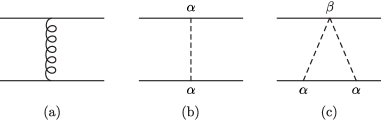
| where is the relative velocity between the two bodies, is their relative displacement, and is the unit vector pointing in this direction. From a diagrammatic viewpoint, the leading term in this potential can be attributed to -channel exchanges of potential-mode gravitons and scalars between the two worldlines, as depicted in figures 2(a) and 2(b), respectively. These two interactions combined give rise to an inverse-square-law force whose overall strength is set by the effective gravitational constant . The remaining terms in (4.10a) are the 1PN corrections, which stem from a total of 11 diagrams (see, e.g., figure 7 of ref. [199]) and can be seen to depend on two constants, and , that are built from combinations of the bodies’ parameters. These symbols are defined in table 2, as are all of the other variables and parameter combinations used in this work. | ||||
| Symbol | Definition | Symbol | Definition |
|---|---|---|---|
| Relative coordinates | |||
| Radiative sector | |||
| Mass combinations | |||
| Spin combinations | |||
| Conservative sector | |||
The leading contribution to the disformal spin-independent sector was recently calculated in ref. [182], albeit only for the special case in which and . It is nevertheless straightforward to repeat the calculation with arbitrary coefficients, in which case one finds
| (4.10b) |
The Feynman diagram responsible for this disformal interaction is shown in figure 2(c).
Now turning our attention to the spin-orbit part of the potential, we find that
| (4.10c) | ||||
| (4.10d) |
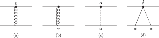
at leading order in , and note that both and swap sign under the interchange of the body labels . The conformal terms in (4.10c) are the result of three Feynman diagrams, as shown in figures 3(a) to 3(c). The first two are the usual contributions from general relativity, which have previously been calculated in ref. [187], while the third diagram in figure 3(c) accounts for the extra effect from the scalar field, whose evaluation is novel to this work. Likewise, the evaluation of figure 3(d), which leads to the disformal terms in (4.10d), is also a novel result. The details of these algebraically lengthy calculations are presented in appendix B.
It is now worth highlighting that these results are written in terms of the spin components and . In this decomposition, our index notation can no longer distinguish between spin tensors defined in different frames; hence, we should clarify that we will always be working with the spin tensor as defined in the locally flat frame, until stated otherwise. The covariant SSC in (3.23) can be rewritten as
| (4.11) |
in this notation, up to corrections that come from projecting the tangent vector onto the locally flat frame [230, 195].181818The vierbein that effects this transformation is , where is the Kronecker delta. These corrections need not concern us at the order to which we are working, however.
4.3 Equations of motion
Potential in hand, the equations of motion for this two-body system now follow from the Euler–Lagrange and Hamilton equations in (2.10). The former tells us that the worldlines trace out trajectories governed by the equation , where the acceleration vector specifies the total force per unit mass acting on the th body. Splitting it up into its four constituent parts as per (4.8), we find that the acceleration of the first body is
| (4.12a) | ||||
| (4.12b) | ||||
| (4.12c) | ||||
| (4.12d) | ||||
to the order at which we are working, and note that we write as shorthand. The acceleration of the second body can then be obtained by simply interchanging the labels , and recall that the vectors and swap sign under this interchange.
To obtain the spin equations of motion, it is useful to first introduce the spin vector as an alternative but equivalent way of encoding the same information as the antisymmetric tensor . The two are related by the identity , and in what follows, we shall often switch between them based on whichever proves more convenient. In terms of these spin vectors, the Poisson brackets in (3.27) read
| (4.13) |
and Hamilton’s equation then tells us that
| (4.14) |
The last term above is the leading contribution in the disformal sector, while the rest make up the leading contribution in the conformal sector. The equation governing the evolution of follows after interchanging the labels .
Worth reiterating is the requirement that the SSC in (4.11) be imposed only at the level of the equations of motion, and not beforehand. Having done so, this explains why the conservative potential in (4.10) depends explicitly on both and , whereas the equations of motion in (4.12) and (4.14) depend only on the latter (or its equivalent, ).
Constants of motion.
These equations fully specify the conservative dynamics of our two-body system at the order to which are working, but are difficult to solve as is, and so motivate us to look for a number of conserved quantities.
To begin with, the fact that the two-body Routhian191919Or, more fundamentally, the two-body Lagrangian . is invariant under spatial translations tells us via Noether’s theorem that the total linear momentum
| (4.15) |
is a constant of motion. Notice that this momentum receives no contribution from the disformal terms in (4.10b) and (4.10d) because any term in that depends on and only via the relative velocity () cancels itself out once we sum over .
Similarly, rotational invariance leads to a conserved total angular momentum
| (4.16) |
The binary’s orbital angular momentum is given by at leading order, while is the sum of the two individual spin vectors.202020At higher orders in the PN expansion, will also depend on the spin variables [267, 268, 269], but these corrections will be of no concern to us here.
Another important symmetry of the Lagrangian is its invariance under Lorentz boosts, which although no longer manifest, is guaranteed by the fact that our EFT in (4.1) is globally Poincaré invariant. Consequently, the vector [270]
| (4.17) |
is conserved order by order in the PN expansion, and since is itself a conserved quantity, differentiation with respect to time tells us that . The vector can thus be interpreted as (being proportional to) the position of the binary’s centre of mass. In our case, it is easy enough to integrate (4.15) directly to find
| (4.18) |
up to an irrelevant additive constant. In arriving at this result, we made use of the equation of motion in (4.12a), but were free to ignore the other three lines in (4.12) as they do not contribute at the order to which we are working. Similarly, the spin can be held constant when going from (4.15) to (4.18), or vice versa, as the time derivative in (4.14) leads to spin-orbit terms that contribute only at next-to-leading PN order.
Combining (4.18) with our definition for the relative displacement, , gives us two equations that can be solved simultaneously for and as functions of and ; thereby allowing us to disentangle the relative motion of the binary from the motion of its centre of mass. Indeed, the latter can be ignored completely by putting ourselves into the centre-of-mass (CM) frame, wherein and . Having done so, we find that the expression for in this frame is
| (4.19a) | |||
| The mass difference , the symmetric mass ratio , and the spin parameter are all defined as in table 2. The expression for then follows after interchanging the labels , and note that , , , and all swap sign under this interchange. | |||
Now combining the condition with the definition gives us another two equations that can be solved simultaneously for and . At the order to which we are working, the result for in the CM frame is
| (4.19b) |
while the result for follows after interchanging the labels . As a consistency check, note that (4.19b) can also be obtained by differentiating (4.19a) with respect to time and then using the equations of motion.
The last constant of motion we shall consider is the binary’s total energy, which can be determined by constructing the two-body Hamiltonian . Having already performed a partial Legendre transform on the spin variables to get to the Routhian, all that remains is to Legendre transform the position variables; hence,
| (4.20) |
Subtracting the rest masses of the two bodies from this Hamiltonian gives us the orbital binding energy , and it is convenient to further define as the orbital binding energy per unit reduced mass. Split into its four constituent parts as per (4.8), we have that
| (4.21a) | ||||
| (4.21b) | ||||
| (4.21c) | ||||
| (4.21d) | ||||
when expressed in the CM frame. The disformal spin-orbit contribution vanishes at the order to which we are working because (4.10d) is linear in the velocities, and so cancels itself out in the Legendre transform. Meanwhile, the conformal spin-orbit contribution is nonvanishing only because of the terms in (4.10c) that are proportional to , and we reiterate yet again that the SSC should be imposed only at the end of our manipulations.
Relative acceleration.
Given the transformation rule in (4.19), we can now simplify the equations of motion by putting them into the CM frame. For the worldlines, we find that the displacement vector evolves according to the equation , where is the relative acceleration between the two bodies. Explicitly, we have that
| (4.22a) | ||||
| (4.22b) | ||||
| (4.22c) | ||||
| (4.22d) | ||||
The spin combinations and are defined as in table 2.
Spin precession.
Applying (4.19) to (4.14) allows us to replace by , but the result is still not in a useful form because it does not preserve the magnitude of the spin vector. One can see this easily by taking the inner product of (4.14) with to find that . However, recall from our discussion in section 3 that the magnitude of the spin tensor is conserved [i.e., ]; hence, it must be that the nonconservation of is simply a coordinate artefact.
Indeed, a simple Lorentz boost in the direction of the body’s motion is all that is required to put (4.14) into the form of a precession equation. The spin vector defined in this comoving frame is related to the spin in the locally flat frame by [187, 189]
| (4.23) |
Making this transformation, using the equation of motion for , and then using (4.19) to replace by , we find that (4.14) ultimately becomes
| (4.24) |
where is the orbital angular momentum vector in the CM frame. As usual, the equation of motion for follows after interchanging the labels .
The fact that the equations of motion automatically conserve the magnitude of makes this spin vector a much more natural variable to work with, and so we shall now switch from working with the spin in the locally flat frame to working with the spin in the comoving frame.212121A natural question that arises in retrospect is whether we could have formulated everything in terms of this comoving spin variable from the outset. We ultimately decided on the approach presented herein (which is a generalisation of the Routhian approach by Porto and Rothstein [190]) as we found it to be the most convenient for our purposes. Nevertheless, as we mentioned below (3.27), there are certainly other ways in which we could have arrived at the same result (up to gauge transformations). For instance, Levi and Steinhoff [192] have shown how one can implement the SSC directly at the level of the action by introducing what are essentially Stueckelberg fields associated with the internal symmetry of the particle’s body-fixed frame, followed by a subsequent transformation of the phase-space variables. Note that this is in stark contrast to the method of this paper, wherein the SSC can be imposed only after the equations of motion are obtained via (2.10). The specific SSC used in ref. [192] is a generalisation of the Pryce–Newton–Wigner SSC [238, 271], and it turns out that the transformed spin variable that satisfies this SSC is closely related to the comoving spin variable defined herein. (To see this, compare (4.23) with eqs. (57)–(59) of ref. [190].) Alternatively, section 11 of ref. [233] (see also ref. [206]) describes how one can work with the comoving spin from the outset, albeit at the level of the equations of motion. This switch is certainly beneficial on a conceptual level, but because the difference between and is of order [see (4.23)], very little actually changes on a practical level; at least, at the order to which are working. Apart from (4.14), which has now been superseded by (4.24), all of the other results in this section remain the same regardless of whether they are written in terms of or . For this reason, we shall further drop the superscript “cmv” in what follows to declutter our notation, and so the symbol will henceforth refer to the spin of the th body as defined in the comoving frame.
4.4 Circular nonprecessing orbits
To conclude this section, we now specialise to binary systems in circular nonprecessing orbits. A binary is said to be nonprecessing if the spins of its two constituents are either aligned or anti-aligned with the orbital angular momentum. In this particular configuration, (4.24) tells us that the spin vectors are individually conserved, and since the total angular momentum is necessarily conserved (when neglecting radiation), it follows that the orbital angular momentum is also conserved. This makes it possible for us to find a solution to (4.22) that describes a circular orbit.
Specifically, what we are looking for is a solution that satisfies the conditions and . We also have that by definition, and this can be used to eliminate all instances of from (4.22); thus leaving us with an implicit equation that relates the orbital frequency to the relative separation . Order by order in our three expansion parameters, we find that the solution to this implicit equation is [note that ]
| (4.25) |
where is the unit vector in the direction of . Notice that there are no disformal spin-independent terms in the above result, as these vanish for circular orbits [181, 182].
A more useful result to have is the inverse of this relation, which reads
| (4.26) |
when written in terms of the post-Newtonian variable
| (4.27) |
For circular nonprecessing orbits, performing a post-Newtonian expansion is tantamount to expanding in powers of this single variable , since we have that on account of the virial theorem. Thus, the order at which a given term contributes can be easily ascertained by simply counting powers of .
Now imposing the conditions for a circular orbit on (4.21), and then using (4.26) and (4.27) to eliminate and in favour of , we finally arrive at the main result of this section. Split into its four constituent parts as per (4.8), the binding energy for a binary in a circular nonprecessing orbit is
| (4.28a) | ||||
| (4.28b) | ||||
| (4.28c) | ||||
| (4.28d) | ||||
Notice as before that there are no disformal spin-independent terms in this result, as vanishes identically for circular orbits [181, 182]. Our results for and , meanwhile, are each given to leading PN order, while the result for is accurate to next-to-leading PN order.
As a general rule, the relative importance of each of these terms can now be estimated by simply comparing their leading powers of . Case in point, we find that the conformal spin-orbit term in (4.28c) is smaller than the leading spin-independent term in (4.28a) by one and a half powers of , and conventionally, we say that the former starts at 1.5PN order relative to the latter. The disformal spin-orbit term in (4.28d), meanwhile, starts at relative PN order, although its contribution to the binding energy is not actually as small as this naive power counting would suggest. This is due to the size of the overall prefactor
| (4.29) |
which we may interpret as being the (cubed) ratio of the binary’s Vainshtein radius to its Schwarzschild radius . For suitably small values of the coupling scale , this ratio can be large enough to counteract the suppression from the additional powers of ; thus allowing (4.28d) to impart a greater contribution to the binding energy than (4.28c).222222Our power-counting scheme can be used to verify that this inverted hierarchy does not invalidate our perturbative expansion. We find that (4.28c) is suppressed by relative to (4.28a), while (4.28d) is suppressed by relative to (4.28a); hence, the disformal spin-orbit interaction can be larger than its conformal counterpart whenever is small enough that . This is still within the regime of validity of our perturbative EFT as long as ; or, in other words, as long as the disformal spin-orbit term is smaller than the leading spin-independent term. In fact, this is precisely why we are keeping track of this disformal spin-orbit interaction.
To close this section, one final remark about the binding energy is worth making. Notice that its general expression for arbitrary orbits in (4.21) has a vanishing disformal spin-orbit part, but is nonvanishing in (4.28d). This difference can be traced back to the leading term in (4.21), which gives rise to the extra disformal terms in question upon use of (4.26) and (4.27); i.e., upon use of the equations of motion. Physically, we may interpret this as saying that the disformal spin-orbit interaction behaves similarly to a magnetic field. While it does not do any work, it can still lead to bound orbits, and a stronger disformal interaction leads to an orbit that is more tightly bound.
5 Radiated power and the gravitational-wave phase
An isolated two-body system eventually coalesces as it emits gravitational and scalar waves. In this section, our goal is to characterise this outgoing radiation and to quantify its impact on the evolution of the binary. We begin by first computing the power radiated into scalar waves in section 5.1, before turning to a discussion of the accompanying gravitational waves in section 5.2. In section 5.3, we then combine these results into a balance law to determine how the phase of the orbit evolves with time. This ultimately feeds into our result for the gravitational-wave phase, which is what our detectors can measure.
Throughout this discussion, our focus will be centred purely on the linear part of the radiative sector, and we will therefore neglect all subleading contributions from nonlinear effects like tail terms. Moreover, as we did in the conservative sector, the key results in this section will be limited to (quasi)circular nonprecessing orbits for simplicity.
5.1 Scalar radiation
Our starting point for the study of scalar waves is the source function , which can be obtained by summing over all Feynman diagrams with one external radiation-mode scalar [see (2.12)]. At the order to which we are working, the spin-independent part of turns out to be localised entirely along the two worldlines, meaning
| (5.1) |
The outgoing scalar waves can thus be understood as being sourced by the periodic motion of a set of scalar charges
| (5.2) |
None of this is new. The first three terms — which together make up the conformal part of this result — have been taken from ref. [199], while a straightforward generalisation of the result in ref. [182] gives us the remaining disformal term. (To clarify, the result in ref. [182] is limited to systems with and , but it is easy enough to repeat the calculation with arbitrary Wilson coefficients.) In the language of Feynman diagrams, the leading conformal term in (5.2) can be seen to arise from figure 4(a), while the leading disformal term comes from figure 4(b). Not shown here are the four other diagrams (see, e.g., figure 8 of ref. [199]) that are responsible for the 1PN corrections in the conformal sector.
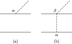
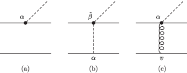
Now turning our attention to the spin-orbit part of , power counting reveals that the leading conformal and disformal terms are given by figures 5(a) and 5(b), respectively. Notice, however, that the diagram in figure 5(a) is proportional to (see table 1), and so vanishes when we impose the covariant SSC in (4.11). As the relevant observables in the radiative sector do not involve any Poisson brackets or functional derivatives, we are free to impose this constraint already at the level of the action; hence, the spin-orbit part of is purely disformal at the order to which we are working. As it so happens, this part is also localised entirely along the two worldlines, as we can write
| (5.3) |
The vectors may be interpreted as scalar dipole moments that are both spin and velocity dependent. Explicitly, we have that
| (5.4) |
having defined and for the sake of brevity. The evaluation of figure 5(b), which is what leads to this result, is novel to this work and is discussed in more detail in appendix B.
Scalar multipole moments.
With in hand, we can now use (2.15) to determine the scalar multipole moments for the binary as a whole. Split into their four constituent parts as per (4.8), we find that
| (5.5a) | ||||
| (5.5b) | ||||
| (5.5c) | ||||
| (5.5d) | ||||
where the result in each line is given to leading order in .232323Only the terms in (2.15) are needed at this order. These expressions should be regarded as being “off shell” in the sense that they currently make no assumptions about the binary’s orbit, apart from requiring that , as is needed to establish the validity of the multipole expansion in (2.14).
What we will do now is put these results “on shell” by going into the CM frame and substituting in the solutions to the equations of motion. For circular nonprecessing orbits, we find that these scalar multipole moments can all be cast into the general form
| (5.6) |
although it must be emphasised that this expression holds only at the order to which we are working. The dimensionless functions are given by
| (5.7a) | ||||
| (5.7b) | ||||
| (5.7c) | ||||
| (5.7d) | ||||
when split into their four constituent parts, with and defined as in table 2. The result in each line is accurate to leading order in , with the exception of (5.7b), which vanishes identically for circular orbits [182].
Two other observations about these results are now worth making. First, notice that while the conformal spin-orbit part is zero off shell [see (5.5c)], it is nonzero on shell. The first term in (5.7c) arises when we use (4.19) to go into the CM frame. This transformation introduces a new term into that is linear in , which must then be reclassified as a new term in . The subsequent use of the equations of motion in (4.26) and (4.27) causes more terms to “leak” from the spin-independent sector into the spin-orbit sector, and is responsible for the remainder of (5.7c), as well as the second term in (5.7d).
That vanishes off shell is, of course, merely an artefact of working at leading PN order. It is nonzero already at next-to-leading order, but for our purposes, these corrections can be safely neglected, since their contribution to is smaller than that of (5.7c). To verify that this is the case, consider just one out of the many Feynman diagrams contributing to at this order. An example is shown in figure 5(c). Power counting tells us that this diagram scales as — the first two factors in parentheses come from table 5, while the extra factor of accounts for the fact that the outgoing scalar is a radiation mode. Now dividing this by and then multiplying by to get its contribution to [cf. (2.14) and (2.15)], we see that figure 5(c) results in a term that scales as . This should be contrasted with the term in (5.7c), whose contribution to scales as , which is indeed one PN order lower.
Our second observation pertains to the order at which different multipoles contribute to the power . In appendix C, we show that the master formula in (2.16a) simplifies to
| (5.8) |
when the on-shell expression in (5.6) holds. The numerical coefficient can be evaluated on a case-by-case basis [see (C.7)], and we find that , , and for the lowest few values of . Written in this way, (5.8) clearly shows that the higher multipole moments are suppressed by increasingly many powers of (), and so contribute less and less to the final result. Consequently, it will generally suffice to keep only the contribution from the dipole moment when working to leading PN order.
There is, however, an important exception to this rule that arises when the binary’s constituents have comparable coupling strengths , as this results in a dipole moment whose spin-independent part vanishes at leading PN order. Said differently, the definitions in table 2 can be used to show that , where , and we must be able to account for the possibility that can vanish if our results are to be as general as possible. To that end, we will now determine which terms must be included in our calculation for when (or is otherwise suitably small) by making a few power-counting arguments. In the spin-independent sector, a cursory glance at (5.7) and (5.8) reveals that the dipole moment contributes a term to that is usually proportional to (plus higher-order corrections), but that becomes proportional to when , since in this case. The size of has no effect on the starting PN order of the other multipole moments, however, and so the quadrupole moment — whose contribution to is always proportional to — takes over as the dominant term when . All of the higher multipoles remain suppressed by additional powers of , and thus can always be neglected when working to leading order.
The situation in the spin-orbit sector is rather different, on account of being built from cross terms of the form . From (5.7) and (5.8), we see that the dipole moment contributes a term in that is usually proportional to , but that becomes proportional to when for the same as reason as before; namely, because in this limit. Meanwhile, the quadrupole moment provides a contribution that is also proportional to regardless of the size of ; hence, both must be included when is suitably small, but only the former is needed otherwise. The same is true in the disformal spin-orbit sector as well, except that the dipolar contribution now scales as or depending on the size of , while the quadrupolar contribution is always proportional to . All of the higher multipoles are consistently suppressed by additional powers of and can therefore be neglected.
This simple power-counting exercise has identified which terms are needed for a complete solution to at the order to which are working, and we now see that in addition to the leading-order expressions in (5.7), we will also require at next-to-leading PN order. Indeed, it is precisely for this reason that we have kept the conformal spin-independent results in section 4 and in (5.2) accurate to 1PN order.
Substituting (5.2) into (2.15) as before, but now keeping the 1PN corrections, we find that the conformal spin-independent part of the dipole moment is
| (5.9) |
Even with these 1PN corrections included, (5.9) can still be cast into the general form of (5.6) thanks to the vanishing of the term and the fact that when evaluated on shell for circular nonprecessing orbits. The same cannot be said of the higher multipoles, but these do not contribute at the order to which we are working. For the dipole moment, we find that
| (5.10) |
to 1PN order after using (4.19), (4.26), and (4.27); with defined as in table 2.
Radiated power.
The power radiated into scalar waves can now be computed explicitly. Following ref. [203], we will account for the possibility that can vanish by splitting the power into a dipolar () and nondipolar () part:
| (5.11) |
The nondipolar part is defined as the set of terms that survive in the limit , while the dipolar part consists of the remaining terms that are all proportional to at least one power of . It is worth noting that this terminology — whilst conventional — is a bit of a misnomer, as and can both receive contributions from multipole moments of any order. In this context, whether a term is deemed to be “dipolar” or “nondipolar” is simply a statement of how it behaves when .
Having split into its dipolar and nondipolar part, we now use (4.8a) to further subdivide each piece into a spin-independent and spin-orbit part. A subsequent decomposition into a conformal and disformal part à la (4.8b) will also be made in the spin-orbit sector, but this will no longer be necessary in the spin-independent sector, as the vanishing of (5.7b) renders it purely conformal in the case of a circular nonprecessing orbit. The end result is thus a division of into six qualitatively distinct parts:
| (5.12) |
Expressions for each will now be determined to leading PN order. We do so by substituting (5.7) and (5.10) into (5.8) while keeping only the leading-order contributions, as identified by our earlier power-counting arguments. The result in the spin-independent sector is
| (5.13a) | ||||
| (5.13b) | ||||
| These expressions are very well known (see, e.g., refs. [197, 199, 203]), but the following spin-orbit results are novel to this work. In the conformal spin-orbit sector, we find that | ||||
| (5.13c) | ||||
| (5.13d) | ||||
| at leading PN order, while in the disformal spin-orbit sector, the leading terms are | ||||
| (5.13e) | ||||
| (5.13f) | ||||
5.2 Gravitational radiation
Besides opening a new channel for radiation, the presence of a light scalar field also causes the amount of power that is radiated into gravitational waves to deviate from the value predicted by general relativity. This occurs for two reasons. First, the gravitational multipole moments, and , inevitably receive new contributions from Feynman diagrams that involve the exchange of one or more potential-mode scalars [see (2.13)]. Second, the scalar’s impact on the binary’s conservative dynamics also affects the final result for , as the solutions to the equations of motion in section 4 are needed when putting and on shell. As it turns out, the former contribution is irrelevant at the order to which we are working, and so we need only concern ourselves with the latter.
Power-counting arguments will be used to substantiate this claim in due course, but we will simply take it as a given for now. If so, then the leading-order (off-shell) expressions for and are the same as in general relativity, and it has already been shown that [233]
| (5.14a) | ||||
| (5.14b) | ||||
at leading order in the spin-independent sector, with . In the spin-orbit sector, the leading terms are [233]
| (5.15a) | ||||
| (5.15b) | ||||
It should be noted that these results are not completely general, as they have already been restricted to the CM frame. Nevertheless, they remain valid for our purposes because the leading spin-independent and spin-orbit terms in (4.19), which are responsible for effecting this transformation, are also the same as in general relativity.
The power radiated into gravitational waves can now be computed by substituting (5.14) and (5.15) into the master formula in (2.16b). Only the quadrupole moments are needed at leading order,242424More precisely, only the mass-type quadrupole moment is needed to calculate at leading order, but both the mass-type and current-type moments are needed to determine , which is built from the two cross terms and . This is because is suppressed by one power of relative to , but conversely, is suppressed by one power of relative to . and for circular nonprecessing orbits we find that
| (5.16a) | ||||
| (5.16b) | ||||
prior to using the equations of motion. To elaborate, we have already imposed the kinematic conditions and to obtain the above result, but have yet to make use of the equation of motion in (4.26), which establishes a dynamical relation between and . Doing so gives us our final result, which reads
| (5.17a) | ||||
| (5.17b) | ||||
| (5.17c) | ||||
We saw previously when computing that the use of (4.26) invariably causes terms to leak from the spin-independent sector into both the conformal and disformal spin-orbit sectors, and this explains why there is now a nonzero disformal spin-orbit part in (5.17c), despite the fact that (5.16) is purely conformal.
Having determined each part of to leading PN order, we are now in a position to verify our earlier claim that the scalar-induced corrections to and contribute only at next-to-leading PN order. To start with, recall from our discussion in section 2 that the key quantity of interest in the gravitational sector is the binary’s energy-momentum tensor . Not unlike how is related to by the master formula in (2.15), analogous formulae exist for relating to the multipole moments and ; see, e.g., eqs. (7.44) and (7.45) of ref. [195] for the explicit expressions. Having said that, the only thing we need to know here is that these master formulae treat the components , , and on unequal footing by virtue of and being tensors, rather than Lorentz tensors. We must therefore power count separately for each of , , and , but since the three cases are qualitatively very similar, we shall present just the first case with below.
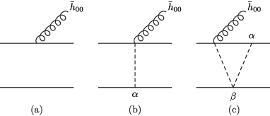
Drawn in figure 6 are a number of Feynman diagrams that contribute to according to the definition in (2.13). Figure 6(a) is the leading term in this series, while figure 6(b) is just one out of several diagrams responsible for the leading correction due to a scalar in the conformal spin-independent sector. Our power-counting rules tell us that
| (5.18) |
where each factor in parentheses comes from either table 1 or table 5, while the extra factors of account for the fact that the outgoing graviton is a radiation mode. Clearly, figure 6(b) is suppressed by one PN order relative to figure 6(a), and will therefore contribute terms to and that are one PN order higher than those in (5.14). Its contribution to is thus also one PN order higher than the leading term in (5.17a), and can therefore be neglected. Meanwhile, figure 6(c) is one out of several diagrams responsible for the leading correction due to a scalar in the disformal spin-independent sector, but these disformal terms all vanish identically for circular orbits [182], and so need not concern us here.
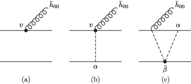
The leading diagram contributing to in the spin-orbit sector is drawn in figure 7(a), while figures 7(b) and 7(c) constitute examples of diagrams responsible for the leading correction from a scalar to its conformal and disformal spin-orbit part, respectively. Our power-counting rules tell us that figure 7(b) is similarly suppressed by one PN order relative to figure 7(a), and will thus contribute terms to that are one PN order higher than those in (5.17b). As for the leading disformal spin-orbit correction, we find that
| (5.19) |
This indicates that figure 7(c) introduces terms into that are suppressed by one power of relative to those in (5.17b), and which therefore scale as overall. In contrast, the leading disformal terms in (5.17c) can be shown to scale as .
One encounters a similar state of affairs when repeating the argument for and , and this allows us to conclude that the scalar-induced corrections to and contribute to only at next-to-leading PN order. Such corrections will not be needed in what follows.
5.3 Balance law and phase evolution
Our result for the total power () can now be used to determine how the binary evolves as it radiates energy into gravitational and scalar waves. The orbit’s response to this energy loss is approximately adiabatic (i.e., ) during the early inspiral, and is therefore well described by the balance law in (2.17). For quasicircular nonprecessing orbits, both the binding energy and the total power depend implicitly on time only through the variable ; hence, the chain rule can be used to recast (2.17) into
| (5.20) |
where . Combining this with the definition for the orbital phase then gives us
| (5.21) |
There are a number of ways in which we could proceed to solve this set of differential equations [272]. The particular approach that we shall adopt here goes by the name of TaylorT2, and entails re-expanding the ratio in powers of to obtain a Laurent series that we can then integrate analytically term by term. What results from this procedure is a pair of parametric equations, and , which together describe how the orbital phase evolves as a function of time. The evolution of the orbital separation then follows immediately from our solution for and the equation for in (4.26).
When solving these equations, care must be taken to distinguish between two substantially different scenarios for the binary’s inspiral. The first possibility is that the binary radiates energy predominantly into dipolar scalar waves, which will be the case whenever is large enough that (5.13a) constitutes the leading term in the total power . Alternatively, if is suitably small relative to , then most of the outgoing radiation will be quadrupolar, and is instead dominated by the sum of (5.13b) and (5.17a). The precise condition that delineates the former dipole-driven regime from the latter quadrupole-driven regime can be determined by comparing the relative sizes of these different terms, and we see that
| (5.22) |
if the system is dipole driven, while must be much greater than if the system is quadrupole driven. (The constant is defined as in table 2.) The fact that the leading term in changes depending on which regime we are in leads to markedly different expansions for the ratio , which must be treated separately.
Dipole-driven regime.
We shall begin with the mathematically simpler case of a dipole-driven (DD) inspiral, for which the leading term in is given by (5.13a). As the remaining terms are all proportional to higher powers of , the ratio can be re-expanded as a Laurent series without any obstruction.
To proceed, it proves convenient to introduce the dimensionless function
| (5.23) |
which is proportional to the rhs’s of both (5.20) and (5.21). Now re-expanding this function in powers of and then truncating to the order at which we are working, we find that the leading term in the spin-independent sector is
| (5.24) |
in agreement with ref. [203]. In fact, has been determined up to relative 2PN order in ref. [203] (albeit in very different, Jordan-frame centric notation), but these higher-order corrections will be of no concern to us here. Instead, what we are interested in are the additional contributions from spin-orbit interactions, and we find that252525To arrive at these results, we made use of the general expression which we then truncated to leading order in after separating it into its conformal and disformal parts.
| (5.25a) | ||||
| (5.25b) | ||||
at leading PN order in the conformal and disformal sector, respectively. The two spin-orbit coefficients and have rather lengthy expressions that can be found in table 3.
| Dipole-driven regime | |
|---|---|
| Quadrupole-driven regime | |
It is now a straightforward task to integrate (5.21) term by term in order to obtain the orbital phase . The end result is schematically of the form
| (5.26) |
where is some integration constant to be fixed by initial conditions, while the other three terms denote the spin-independent, conformal spin-orbit, and disformal spin-orbit parts of the phase, respectively. At leading PN order in each sector, we find
| (5.27a) | ||||
| (5.27b) | ||||
| (5.27c) | ||||
The solution for follows from a similar calculation, and is presented in appendix D.
As we did with the binding energy in section 4.4, we can now determine the relative importance of each term in by simply comparing their leading powers of . We find that the conformal spin-orbit term in (5.27b) starts at 1.5PN order relative to the leading spin-independent term in (5.27a), while the disformal spin-orbit term in (5.27c) starts at relative 4.5PN order, although it is enhanced by the large prefactor , which enters via the definition of the spin-orbit coefficient (see table 3). Per our discussion below (4.29), it follows that for sufficiently small values of , the disformal term in (5.27c) could have a significantly larger impact on the orbital phase than its conformal counterpart, despite the suppression by three additional powers of . This same enhancement of the disformal sector is also present in quadrupole-driven systems, as we shall see.
Quadrupole-driven regime.
A binary is said to be in a quadrupole-driven (QD) inspiral whenever the sum of (5.13b) and (5.17a) serves as the leading term in . In this regime, the re-expansion of requires more thoughtful consideration because of the scalar dipole term in (5.13a), which — on account of the smallness of [see our discussion below (5.22)] — provides only a subleading correction to the overall energy loss, despite being proportional to one less power of than the leading quadrupole term.
Following ref. [203], we will account for this complication by splitting the total power into a dipolar and nondipolar part, as we did for in (5.11). This allows us to write
| (5.28) |
after expanding to first order in the small ratio , where
| (5.29) |
The approximation in (5.28) naturally causes to split into a dipolar and nondipolar part as well, and this motivates writing , with
| (5.30a) | ||||
| (5.30b) | ||||
Both parts of can now be re-expanded in powers of without any further obstructions, and we find that
| (5.31a) | ||||||
| (5.31b) | ||||||
| (5.31c) | ||||||
with the result in each sector given to leading order in . As was the case in the dipole-driven regime, the leading spin-independent terms in (5.31a) are found to be in complete agreement with the results of ref. [203], while the leading spin-orbit terms in (5.31b) and (5.31c) are novel to this work.262626To elaborate further, we obtained the spin-orbit results in (5.31) by starting with the general expressions which we then truncated to leading order in after separating them into conformal and disformal parts. The four spin-orbit coefficients appearing in these results have rather lengthy expressions that can be found in table 3.
We can now integrate (5.21) to obtain the orbital phase , which schematically reads
| (5.32) |
The integration constant is to be fixed by initial conditions, while the remaining terms correspond to a subdivision of the phase into dipolar and nondipolar, spin-independent and spin-orbit, and conformal and disformal parts. At leading PN order in each sector, we find
| (5.33a) | ||||||
| (5.33b) | ||||||
| (5.33c) | ||||||
The solution for follows from a similar calculation, and is presented in appendix D.
Comparing the different powers of in (5.33) gives us an estimate for the relative importance of each term. In the spin-independent sector [see (5.33a)], it is well known that the term proportional to , which arises due to quadrupole radiation, is responsible for the dominant contribution to the phase, while the dipolar term — despite appearing at relative PN order — provides only a subleading correction to on account of the smallness of . This much is guaranteed by definition, as a binary is said to be in a quadrupole-driven inspiral if and only if [or more precisely, if ; cf. (5.22)].
Interestingly, what occurs in the spin-orbit sector can be rather different. To illustrate this, we find it helpful to distinguish between two extreme cases: when and are comparable to one another, such that and ; and when and are vastly different, such that while . Consider the first case with , and take the conformal spin-orbit sector in (5.33b) to start with. Its nondipolar part appears at PN order relative to the leading term in , while its dipolar part starts earlier at relative PN order, but is suppressed due to the smallness of . Crucially, however, we see from table 3 that it is suppressed by only one power of ,272727While has an overall factor of out front, the first term in square brackets is proportional to . unlike , which is suppressed by two. What this means is that the dipolar spin-orbit term () can actually be larger than its nondipolar counterpart () if satisfies the inequality . The value of will continue to increase towards unity as the binary evolves, and the two terms become comparable to one another when . Subsequently, the nondipolar part takes over as the larger contribution when . The same conclusion holds also for the disformal spin-orbit sector in (5.33c), whose dipolar and nondipolar parts start at relative PN and relative PN orders, respectively.
Now consider the second case with and . The dipolar coefficients and go from being suppressed by one power of to being suppressed by two as a result of , , and themselves becoming newly proportional to (cf. table 2). Whether these dipolar terms can ever be larger than their nondipolar counterparts is now a question of what happens to and . In the conformal sector, the coefficient remains of order one, and thus the dipolar term () is always subleading to its nondipolar counterpart (), since we must have in the quadrupole-driven regime. On the other hand, goes from being of order one to being of order when we set and ; hence, the dipolar term () in the disformal spin-orbit sector is always larger than its nondipolar counterpart (). This difference can be attributed to the fact that contains the usual spin-orbit contributions from general relativity in addition to those from a scalar field, whereas is induced purely by the scalar. All of this serves to illustrate how varied the evolution of can be in a scalar-tensor theory when spin-orbit effects are taken into account.282828It goes without saying that these conclusions were drawn by simply counting powers of . Nevertheless, we do not expect them to change on a qualitative level were we to undertake a more deliberate calculation that accounts for all of the different numerical factors in table 3.
As a last remark on (5.33), it is worth reiterating what was said earlier in our discussion below (4.29) and (5.27); namely, that although the disformal spin-orbit sector is suppressed by PN orders relative to the conformal spin-orbit sector, the former can still have a greater impact on the orbital phase as a result of being multiplied by the large prefactor . We will see this explicitly in the next section when we discuss observational prospects, but for now, there is one final step to take in our EFT pipeline.
Gravitational-wave phase.
What we ultimately measure is the gravitational-wave signal from an inspiraling binary, and as we discussed towards the end of section 2, the phase of this gravitational wave derives directly from the binary’s orbital phase . Specifically, after decomposing the signal into spin-weighted spherical harmonics, one finds that the phase of the mode is given by , up to higher-order corrections that we shall neglect [233, 203]. The pair of parametric equations and therefore provides us with our final result for the evolution of the gravitational-wave phase.
This time-domain solution will suffice for our purposes in the next section, although it is worth noting that frequency-domain waveforms are much more convenient for a matched-filtering analysis. If is the waveform for a particular oscillatory mode in the time domain, its counterpart in the frequency domain is given by the Fourier transform
| (5.34) |
Because these gravitational waves are rapidly oscillating but slowly chirping signals, the integral in (5.34) can be evaluated analytically within the stationary-phase approximation. The result is of the general form , where the corresponding phase in the frequency domain is given by [203]
| (5.35) |
Explicit expressions for the leading spin-independent, conformal spin-orbit, and disformal spin-orbit parts of are presented in appendix D. Written in this form (which is known as the TaylorF2 approximant [272]), our results are now ready to be used in model-independent frameworks for testing gravity, like the parametrised post-Einsteinian (PPE) or generalised inspiral-merger-ringdown (gIMR) formalisms [273, 274, 2], or can otherwise be incorporated directly into dedicated waveform models for scalar-tensor theories [203].
6 Double neutron stars and observational prospects
Mention has already been made of the large prefactor , which can cause the disformal spin-orbit terms in the waveform to be enhanced relative to those in the conformal spin-orbit sector. Our goal in this penultimate section is to be more quantitative about the extent of this enhancement, and to investigate if gravitational-wave detectors are capable of observing these interactions as a result. To be clear, gravitational waves are by no means the only avenue for probing these kinds of effects, and need not even be best suited to the task [144] — they are simply the most natural option to consider here, given the collection of results derived in this paper. (We comment briefly on other potential probes in the next section.) The question of how well scalar-tensor theories can be constrained by gravitational waves is nevertheless an interesting and timely one, and so warrants some investigation.
We will be interested primarily in the prospect of probing disformal effects, since the smoking gun for a conformal coupling between a binary and a light scalar field is already well understood: it is the emission of scalar dipole radiation, which has been discussed extensively in, e.g., refs. [143, 144, 145, 146, 147, 148, 149, 150, 151, 41, 42, 43]. As these studies emphasise, a robust assessment of detectability requires deliberate consideration of many factors, like the various degeneracies between parameters, expected detection rates for different binary populations, the signal-to-noise ratio of individual events, and so on. A fully fledged Bayesian approach of this kind, however, is well beyond the scope of this already very lengthy paper; hence, as a precursor to a more in-depth analysis in the future, we shall here employ a more rudimentary diagnostic for assessing detectability. Let be the total number of gravitational-wave cycles that accumulate in the detector as a signal passes through. Following the logic of ref. [143], we deem a particular effect or interaction to be undetectable if its contribution to — integrated over the entire time that the signal spends in the detector’s sensitivity band — is less than , and conversely, we say that it is (potentially) detectable if its contribution to is greater than .
Double neutron stars.
As for the question of which systems are most relevant to our discussion, the choice to focus on double neutron star binaries is essentially forced upon us by two determining factors. The first is the fact that, for the class of scalar-tensor theories considered in this paper, disformal effects enter into the gravitational waveform only if both constituents of the binary are composed of matter. The second is our restriction to circular orbits, which — as far as gravitational-wave sources are concerned — is an assumption that is generally valid only for binaries approaching the end of their inspiral [275, 276, 277]. Taken together, these considerations naturally direct our attention towards double neutron star binaries, which are the only systems (that we know of) whose constituents are both composed of matter and whose inspiral comes to an end within the sensitivity band of a gravitational-wave detector; namely, one that is ground-based.
In this frequency window, the evolution of the binary can be split broadly into three phases: what we will call the perturbative inspiral phase, the nonperturbative inspiral phase, and the merger phase. Mathematically, we write
| (6.1) |
The first of these phases corresponds to the early portion of the inspiral, during which all three expansion parameters — , , and — remain small.292929For noncircular orbits, we would also require ; recall our discussion in section 4.1. The second phase has no analogue in general relativity, and moreover is present only if the disformal coupling scale is below some critical value. This is because the ladder parameter [] grows as the inspiral progresses, and for sufficiently small values of , there will come a time when the combination is large enough to invalidate our perturbative expansion. As we discussed towards the end of section 4.1, the point-particle approximation of the two bodies remains valid in this nonperturbative regime, but maintaining an accurate description of the binary’s dynamics requires a certain class of “ladder diagrams” to be resummed. Finally, the merger phase begins when the two neutron stars come into sufficiently close contact that their orbit becomes unstable, prompting them to plunge into one another [278, 279, 280].
It will be useful in what follows to know approximately when a binary transitions from one phase to the next. To that end, let and denote the gravitational-wave frequencies that mark the beginnings of the nonperturbative inspiral phase and merger phase, respectively. The latter invariably depends on the parameters of the system and on the specific details of the neutron stars’ equation of state [278], but as a rough guide, we shall here adopt a fixed value for . Meanwhile, we can obtain an estimate for by appealing to the fact that the combination is small — or more precisely, that the condition in (4.9) holds — at all frequencies below this threshold. If we further focus on the dominant mode of the gravitational-wave signal for simplicity, we can make the identification , which allows (4.9) to be rewritten as
| (6.2) |
after also defining and making use of (4.26) and (4.27). Moving forward, we shall replace the vague condition “” by the inequality “” to be more concrete, and will take to be our criterion for what we consider small. The quantity is then defined as the frequency that saturates this inequality, and we have that
| (6.3) |
It now follows that a neutron star binary undergoes all three phases as described below (6.1) if , but if , then the binary transitions directly from the perturbative part of its inspiral into the merger phase.
Dephasing.
The results of section 5 enable us to compute only the number of gravitational-wave cycles that accumulate during the early, perturbative part of the binary’s inspiral, but this will nevertheless suffice for obtaining a rough estimate of detectability. The reason being: an effect that contributes more than one cycle to necessarily also contributes more than one cycle to . We can thus revise our criterion for detectability and will now deem an effect to be (potentially) detectable if its contribution to is greater than 1.
Focusing on the dominant mode of the gravitational-wave signal, we have that
| (6.4) |
where the initial time is the time at which the signal enters the detector’s sensitivity band, while the final time marks the end of the perturbative inspiral phase. For the former, we take [cf. (5.35)], and following ref. [41], we consider three possible values for :
| (6.5) |
The largest of these frequencies marks the beginning of the sensitivity band for Advanced LIGO [281], while the remaining two are the projections for future, third-generation ground-based detectors like Cosmic Explorer (CE) and the Einstein Telescope (ET) [282]. As for the end of the perturbative inspiral phase, we take with
| (6.6) |
Note also that if ; in which case, the perturbative part of the inspiral occurs outside the detector’s window.
Having specified the appropriate frequency band, we can now write down an explicit expression for . Current observations of binary pulsars already place strong constraints on the size of [41, 42, 43], which limit the inspiral of a binary neutron star to be quadrupole driven by the time it enters the LIGO/CE/ET band, even if it did undergo a previous dipole-driven phase at lower frequencies. Accordingly, only the formula for in (5.33) is needed to evaluate (6.4). The result can be split into four parts,
| (6.7) |
where the first term is the prediction of general relativity, while the remaining three terms specify the amount of dephasing that accrues in the signal due to the presence of the scalar. Expressions accurate to leading PN order will suffice for an adequate estimate of the size of each of these terms, and it therefore suffices to write
| (6.8a) | ||||
| (6.8b) | ||||
| (6.8c) | ||||
| (6.8d) | ||||
For each sector in , we have included both the leading dipolar part and the leading nondipolar part of the result, as either one can provide the dominant contribution, depending on the relative sizes of and . (Recall our discussion in section 5.3.) Note also that in (6.8b) and (6.8c), the terms proportional to powers of serve to remove the parts of and that overlap with general relativity, since these are already included in ; even if not explicitly written down.
Numerical estimates.
| Weakly scalarised, slowly spinning (W) | |||
| Strongly scalarised, slowly spinning (S) | |||
| Strongly scalarised, rapidly spinning (S∗) |
We now evaluate (6.8) using a selection of parameter values that are typical of neutron stars, as shown in table 4. To explore an array of different possibilities, we have chosen to distinguish between neutron stars that are either weakly or strongly scalarised, and between neutron stars that are either slowly or rapidly rotating. (We leave a more exhaustive exploration of parameter space to future work.) Recalling our discussion at the end of section 3.2, we define a “weakly scalarised” neutron star as one whose coupling strength is equal to up to an order-one factor, while a “strongly scalarised” neutron star is one that has undergone spontaneous scalarisation. Of course, this latter possibility occurs only in a certain class of scalar-tensor theories [34, 35, 36, 37, 38, 39, 40, 54, 55, 56, 57, 58, 59], and only if the mass of the body lies in a suitable range [41, 42, 43, 44]. (Theories that allow for spontaneous scalarisation also lead to a related phenomenon known as dynamical scalarisation [64, 65, 66, 67, 68, 69, 70, 71], but we have neglected this added complication here for the sake of simplicity.)
The corresponding values of in table 4 have been lifted from refs. [41, 42, 43], and are consistent with current constraints from binary pulsars and the gravitational-wave event GW170817.303030Strictly speaking, the upper bounds on in refs. [41, 42, 43] apply only to the specific theory by Damour and Esposito-Farèse [34, 35], but for the sake of illustration, we shall here assume that these values are also representative of the bounds on other models. We further note that our definition for differs from that of refs. [34, 35] by a factor of ; namely, . The minus sign is irrelevant, however, as the effective action in (2.3) is invariant under the transformation . The values of , meanwhile, were obtained by making use of the double pulsar PSR J0737-3039A/B [84], which is presently the only binary neutron star system for which the spins of both components are known. Following ref. [41], we use a combination of their measured spins and spin-down rates to infer the would-be values of when the binary enters the LIGO/CE/ET band, about 86 Myr from now. The three types of neutron stars in table 4 are then used to construct three different types of binary systems, and for each one, we plot the magnitudes of , , , and as functions of in figure 8.
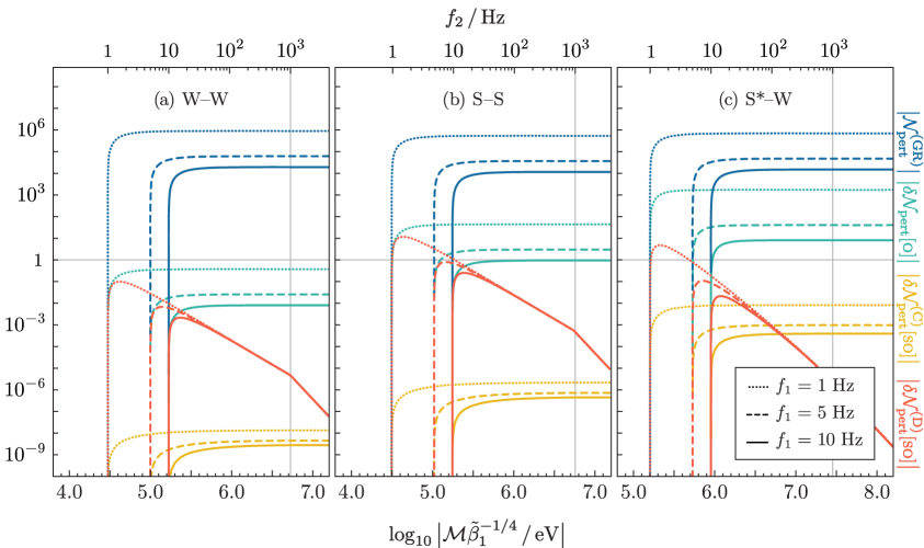
The different curves have qualitatively similar shapes across all three panels that are easy enough to explain. Beginning with , we see from (6.8d) that this quantity is proportional to positive powers of , and thus has its value determined predominantly by the higher frequency . A vertical grey line in each panel marks the critical value of above which , and in so doing, naturally divides the parameter space into two halves. On the right, we have that , and thus , since its dependence on in this region stems solely from the disformal spin-orbit coefficients in table 3. The slope of this curve then changes abruptly when we cross over to the left of the vertical line, where , on account of itself being a function of [see (6.3)]. Depending on whether its dipolar or nondipolar part dominates, is now proportional to either or (or more generally, a linear combination of the two). Its magnitude continues to rise as we move to even lower values of , until approaches , at which point must necessarily vanish. As for the other three terms in , we see from (6.8) that they are all proportional to negative powers of , and thus have their values determined predominantly by the lower frequency . They are mostly independent of as a result, except for when the diminishing difference between and similarly causes them to vanish.
Having understood these qualitative features, we can now comment on the actual magnitudes of these quantities. To start with, consider the binary in figure 8(a), which consists of two identical neutron stars that are both weakly scalarised and slowly rotating. For all three values of , we see that not one of , , or results in a dephasing that is large enough to be detectable; indicating that both current and future ground-based detectors will be unable to distinguish this kind of system from its counterpart in general relativity. Naturally, this begs the question as to what is actually needed for there to be a discernible effect from the scalar field. Being interested particularly in the disformal spin-orbit sector, we shall here consider the requirements for to surpass the threshold value of 1.
A brief inspection of table 3 tells us that we can boost the magnitude of the spin-orbit coefficients and by increasing either the magnitudes of or . We find when repeating the calculation with larger spins up to the Kerr bound (i.e., for all values of ), however, that consistently remains smaller than 1. This might seem surprising at first glance, given that in figure 8(a), already achieves a maximum value of despite the minuscule value of . The reason is simply that also varies with [see (6.3)]. Accordingly, while a larger spin does increase the overall size of the effect, there is a concomitant reduction in the value of , which shortens the amount of time that the binary spends in the perturbative part of its inspiral, and so lowers the number of gravitational-wave cycles that can accumulate during this phase. (Of course, our perturbative results do not preclude the possibility of a large dephasing during the nonperturbative part of the inspiral, although we shall refrain from making any speculations about this regime until a concrete calculation has been achieved.)
The other option to boost is to increase the value of , which is possible if at least one of the neutron stars has undergone spontaneous scalarisation. Shown in figure 8(b) are the number of gravitational-wave cycles that would accumulate in the detector if the binary were composed of two identical, strongly scalarised and slowly rotating neutron stars. Meanwhile, figure 8(c) shows the corresponding values for an asymmetric binary involving one strongly scalarised, rapidly rotating neutron star and one weakly scalarised, slowly rotating neutron star.313131For the asymmetric binary, we take to correspond to the more massive, strongly scalarised star. Moreover, to properly evaluate each part of in this case, we must also specify appropriate values for the Wilson coefficients and . This was not necessary for binaries with identical constituents, since in that case, while (which enters via the definition of ) is always multiplied by something that vanishes. For the asymmetric binary, we find that the curves in figure 8(c) are mostly insensitive to the precise value of and as long as , , and . For this latter case, our choice to furnish the more massive object with the larger spin is informed by the standard picture of binary neutron star formation [283, 280]. In short, the more massive constituent of what is initially a main-sequence binary is the first to undergo core collapse and leave behind a neutron star. This neutron star then gains mass and angular momentum when its companion evolves off the main sequence and overflows its Roche lobe. Eventually, the companion also collapses to form a neutron star, but the preceding period of mass transfer guarantees that this secondary neutron star is always lighter and more slowly rotating than the primary.
As promised, the larger value of does indeed lead to a larger value of . While the amount of dephasing is still too small to be detectable by current gravitational-wave detectors, figure 8 suggests that:
A future detector like the Einstein Telescope will be sensitive enough to probe disformal spin-orbit effects in a narrow range of values for if at least one of the binary’s constituents is strongly scalarised.
A comparison between figures 8(b) and 8(c) further reveals that while the magnitudes of the spins have little impact on the maximum value of (for reasons already discussed), their impact on the value of leads to a discernible shift in the position of this maximum. Case in point, the small and large values of in table 4 result in a sensitivity window to that is peaked around 40 keV and 200 keV, respectively.
As a final remark on figure 8, it is worth noting that while can become greater than 1 for suitably small values of , remains significantly less than 1 in all three panels. When combined with the fact that the values of in table 4 are meant to be representative of typical neutron star spins, while the values of are the largest possible given existing constraints, these results indicate that both current and upcoming ground-based detectors will be insensitive to the effects of a scalar-induced, conformal spin-orbit interaction in (the perturbative part of) a binary neutron star inspiral. This conclusion is in complete agreement with the expectations we laid out in section 1. Note, however, that the magnitudes of and could be much larger in binary systems of scalarised black holes; hence, our perturbative results for the conformal spin-orbit sector may still play an important role in the modelling of such systems. We will comment briefly on this scenario in section 7.2.
Caveats.
For now, let us close this section by highlighting several of its limitations. First, it almost goes without saying that the small selection of values in table 4 leaves most of parameter space unexplored. Because different models lead to different predictions for how the Wilson coefficients depend on the properties of the neutron star and the underlying parameters of the scalar-tensor theory, it is difficult to perform a meaningful exploration of parameter space without also being explicit about the specific details of the microscopic physics. In lieu of this, we have elected to simply use the small number of illustrative values in table 4 to make some generic statements about the detectability of disformal spin-orbit effects. Our expectation is that these conclusions are fairly representative of a broad class of models, but it is certainly possible that some models could give rise to larger effects that can already be constrained by current-generation detectors, and conversely, there will surely be others whose imprints are too small to be observable by any planned detector. It would therefore be valuable in the future to map our general results for the gravitational-wave phase onto specific models, so as to establish more definitive constraints.
Second, recall that in addition to the masses, spins, and Wilson coefficients of the two bodies, our formula for also takes as input a value for the small parameter [see (6.3)], which sets the criterion for when we think our perturbative ladder expansion breaks down. The results in figure 8 assume a value of , and while we believe this to be a fairly conservative choice, it should be noted that our conclusions turn out to be quite sensitive to this particular parameter. A value of , for instance, would mean that even current-generation detectors can be sensitive to disformal spin-orbit effects in strongly scalarised binaries of the kind in figure 8(b), while an even larger value of would allow for a future detector like the Einstein Telescope to see the imprints of a disformal spin-orbit interaction in weakly scalarised binaries of the kind in figure 8(a). Going in the opposite direction, we find that for , all three of the ground-based detectors considered in this section would be blind to disformal effects during the perturbative part of the binary’s inspiral. It would therefore be instructive to extend our calculations to higher orders in the disformal coupling in the future, so that we can refine our estimate for when our perturbative expansion breaks down; or, better yet, one could consider exploring how to resum the relevant set of ladder diagrams, so as to obtain a reliable prediction for both the perturbative and nonperturbative parts of the binary’s inspiral.
Finally, it is worth reiterating that our rudimentary criterion for detectability in this section does not account for several important factors, like the inevitable degeneracies between parameters, expected detection rates, signal-to-noise ratios, and so on. Indeed, we know that in the spin-independent sector, the green lines in figures 8(a) and 8(b) overestimate how likely we are to detect the presence of a scalar in systems with , as the absence of scalar dipole radiation means that is degenerate with a rescaling of the total mass at leading PN order. One therefore has to rely on the corrections from higher-PN-order terms to break this degeneracy, but these higher-order terms are naturally harder to constrain, given that they are suppressed by one or more powers of . For , we can already see from table 3 that a measurement of is degenerate with a rescaling of , since these quantities only appear in the combination . This should not prevent us from detecting the presence of a disformal spin-orbit interaction, should one exist with a favourable value of , but it is unlikely that the data can be used to pinpoint the exact value of , unless it can separately pinpoint the values of . (Note that thus far, all of the neutron stars that have been detected through gravitational waves have spins that are either unconstrained or only weakly bounded from above [284, 285, 286].) On the whole, these limitations motivate undertaking a more robust, Bayesian analysis in the future.
7 Discussion
7.1 Summary of main results
In this work, we used a generalisation of the NRGR approach [183, 184, 185, 186, 187, 188, 189, 190, 191, 192, 193, 194, 195, 196] to compute the leading spin-orbit effects that would arise when a compact binary is coupled both conformally and disformally to a light scalar field. After reviewing the main conceptual ideas in section 2, we showed in section 3 how one could construct a general point-particle action for spinning bodies in this class of theories by utilising a two-step approach. Our first step was to perform a frame transformation on the corresponding action in general relativity as a means of systematically generating new terms that couple the effective point particle directly to the scalar field. The result of this procedure suffices as a model for how weakly gravitating bodies behave (when viewed from large distances) in the Einstein frame, but for strongly gravitating objects like black holes and neutron stars, a second step where we generalised the action to allow for arbitrary values of the Wilson coefficients was required. This extra step accounts for the fact that when a body has a considerable amount of self-gravity, the strength with which it couples to the scalar is largely influenced by the microscopic details of its interior. The precise relation between a body’s Wilson coefficients and its internal structure can be determined on a case-by-case basis by performing a number of matching calculations (see section 3.2 for examples), but for most of this paper, we have left these coefficients as free parameters, thereby rendering our results general enough to describe any spinning body [up to subleading effects that we neglect; see the discussion below (3.16)]. The final result of this section is given in the form of a Routhian in (3.25).
In section 4, two distinct copies of this Routhian were combined with our fiducial field action to produce the total effective action in (4.1). With the help of Feynman diagrams, we then integrated out the potential modes of the scalar and gravitational field from this action to arrive at a perturbative result for the two-body potential , which we divided into four “sectors” according to (4.8). The result itself is given in (4.10). A mixture of Euler–Lagrange and Hamilton equations were then used to derive the conservative equations of motion for this system, which are given by (4.22) and (4.24) when expressed in the centre-of-mass frame. Finally, we concluded our discussion of the conservative sector by specialising to circular nonprecessing binaries in section 4.4. The orbital binding energy for systems in this particular configuration can be found in (4.28).
Turning to the radiative sector, in section 5.1 we used a similar diagrammatic technique to compute the multipole moments [see (5.5)] that are responsible for sourcing outgoing scalar waves. The amount of power that is carried away by these waves is given in (5.13), assuming again that the binary is in a circular nonprecessing orbit for simplicity. In section 5.2, we then used power-counting arguments to show that the gravitational multipole moments and are the same as they would be in general relativity (at the order to which we are working), although the presence of a scalar does contribute indirectly to the power radiated into gravitational waves via the solution to the conservative equations of motion, which is needed to put the result “on shell.” For circular nonprecessing binaries, the result for is given in (5.17). Finally, in section 5.3, we combined these results for the total power with our earlier expression for the orbital binding energy to determine the evolution of the binary’s orbital phase , and by extension, its gravitational-wave phase (up to nonlinear radiative corrections like tail terms, which we neglect).
Care was taken to distinguish between two possible scenarios: a dipole-driven inspiral, wherein the binary loses energy predominantly to scalar dipole radiation, and a quadrupole-driven inspiral, during which energy is radiated mostly into the quadrupolar modes of the scalar and gravitational field. The results for these two cases are given in (5.27) and (5.33), respectively, when expressed in the time domain, while the corresponding frequency-domain results can be found in (D.4) and (D.8). We should clarify that our results for the latter, quadrupole-driven regime will be the most relevant for establishing constraints if our default assumption is the validity of general relativity, but because current observations do not yet preclude the possibility of a binary that undergoes a (temporary) dipole-driven phase during the very early stages of its inspiral, we have made allowances for this more exotic scenario as well.
At this stage, it is useful to mention a number of consistency checks that have been performed to validate the results of this paper. First, note that none of our results in the conformal spin-independent sector are new, as they have been lifted directly from refs. [197, 198, 199]. Additionally, note that the leading effects (both conservative and radiative) from a disformal spin-independent coupling have previously been calculated in refs. [181, 182], albeit only for the special case in which and . Our results for this sector correctly reduce to those of refs. [181, 182] when we take this limit, but we think it is important to stress that our results are more general, as they also allow for body-dependent Wilson coefficients, which are necessary when modelling systems of strongly gravitating objects.
That said, the key novelty of this work is the calculation of the additional spin-orbit effects that are induced by a conformal and disformal coupling to the scalar field. Some preliminary results in this direction can be found in a previous paper of ours; namely ref. [206], although we restricted ourselves to a conservative setting in that study and, moreover, focused only on weakly gravitating bodies. We have checked that the more general results of this present work correctly reduce to those of ref. [206] after setting and ,323232To translate our results into the notation of ref. [206], set and . but note that this only validates our results in the conservative sector. To the best of our knowledge, our results for the scalar-induced, spin-orbit parts of the radiated power and gravitational-wave phase have been calculated here for the very first time. (Of course, the conformal spin-orbit sector has a part that overlaps with general relativity, and we have verified that this subset of terms is consistent with the results in ref. [233].)
To illustrate that these effects are not merely theoretical curiosities, but are also relevant for phenomenological applications, we concluded this paper by assessing their observational prospects in current and future ground-based, gravitational-wave detectors. The results of section 6 suggest that a future detector like the Einstein Telescope will be sensitive enough to probe disformal spin-orbit effects in double neutron star binaries for values of in the to keV range if at least one of the two bodies is sufficiently scalarised. This is encouraging, although as we highlighted towards the end of section 6, our rudimentary analysis leaves several important factors (like the various degeneracies between parameters) unaccounted for, and thus this preliminary result should be taken mostly as motivation for performing a more robust, Bayesian analysis in the future.
7.2 Future directions
Additionally, some other key directions for future work are as follows.
Amplitude corrections.
Because a matched-filtering analysis is much more sensitive to variations in the phase than in the amplitude of the gravitational wave, we have concentrated only on the former in this work. This should suffice for placing order-of-magnitude constraints on new physics [287], but if (or when) a deviation from general relativity is found, both amplitude and phase corrections should be included in the waveform to minimise systematic errors.
Going beyond the ladder expansion.
The inspiral phase of a binary system splits into a perturbative and nonperturbative part when the disformal coupling scale is small enough to be of phenomenological interest [see the discussion around (6.1)]. Because the results of this paper were truncated to first order in the disformal coupling (i.e., to first order in ) for simplicity, its predictions are valid only in the former perturbative regime. Constructing a waveform that remains valid over the entire course of the inspiral would be highly desirable, but this rests on our ability to gain a good handle on the nonperturbative regime, which entails being able to resum a certain class of ladder diagrams. Fortunately, this has previously been shown to be possible for systems of nonspinning bodies [265, 266], and it is likely that similar techniques could also be used to address the spinning case.
Other observational probes.
As a precursor to more extensive studies in the future, our discussion in section 6 focused solely on the constraining power of ground-based detectors. It would be interesting to explore how much we could learn from future space-borne missions, like the Laser Interferometer Space Antenna (LISA) [288] or the Decihertz Interferometer Gravitational Wave Observatory (DECIGO) [289]; and also, to examine what constraints can be placed by using observational data of binary pulsars [290, 291, 292]. We expect that each of these experiments will have their uses, since they are sensitive to binaries within a different range of orbital frequencies. Accordingly, they will be sensitive to different values of the coupling scale , and thus will cover complementary regions of parameter space. Note, however, that the results of this paper should be generalised to include a nonzero eccentricity before applying them to the above cases, since binary systems with lower orbital frequencies have yet to fully circularise.
Orbital precession.
Another generalisation we could make in the future would be to relax our assumption of a nonprecessing orbit. In particular, so-called “up-down binaries” are known to be unstable to small perturbations in the orientations of their spins [293, 294, 295, 296], and it would be interesting to see what effect a disformal spin-orbit interaction might have on this instability.
Spinning black holes.
While the tail end of this paper focused primarily on the prospect of observing disformal spin-orbit effects in double neutron stars, it is worth reiterating that the general results in sections 3 to 5 can also be used to describe systems of “hairy” black holes. Such objects would not be affected by a disformal coupling, but our results in the conformal spin-orbit sector still apply. With a minimal amount of effort (mostly needed to square differences in notation), these can be combined with the spin-independent results of refs. [60, 61, 62, 63] to produce 1.5PN-accurate waveforms for spinning black hole binaries in Einstein-scalar-Gauss-Bonnet theories.333333Our field action in (4.2) does not include the all-important term that couples the scalar to the Gauss-Bonnet invariant, but from power counting we know that we only need its contribution in the spin-independent sector (which is already given in refs. [61, 62, 63]) to obtain accurate spin-orbit results at leading order.
Constraining gravity on multiple scales.
By treating the masses, spins, and Wilson coefficients of the two bodies as free parameters, our results are general enough to describe how spinning compact binaries evolve in a broad class of scalar-tensor theories. There is, however, only so much information that can be gleaned from placing constraints on Wilson coefficients; hence, as we discussed at the end of section 6, it would also be interesting to apply our results to specific models. Performing the requisite matching calculations that link the two bodies’ Wilson coefficients to the underlying parameters of the scalar-tensor theory would then allow us to establish more definitive constraints on those model parameters directly. This would also allow us to explore how the constraints on conformal and disformal couplings that derive from compact binaries compare with those that have already been established in the Solar System [73, 74, 75, 76, 206] and on much larger cosmological scales [87, 88, 89, 134, 135, 136, 137, 138, 139, 140, 141, 142].
Nonlinear interactions.
It is important to appreciate, however, that viable cosmological models typically rely on nonlinear interaction terms in the field action to screen their effects on smaller scales (see refs. [76, 80, 297] for modern reviews), but such terms were omitted in this work for simplicity. The impact of scalar self-interactions on the evolution of a binary is not fully understood, and remains an active area of research [219, 220, 221, 222, 223, 224].
Acknowledgments
This project has received funding/support from the European Union’s Horizon 2020 research and innovation programme under the Marie Skłodowska-Curie grant agreement No. 860881-HIDDeN. This work was partially supported by STFC consolidated grants ST/P000681/1 and ST/T000694/1. S.M. is supported by a UKRI Stephen Hawking Fellowship (EP/T017481/1). The xAct package [298] for Mathematica was used to aid some of our calculations.
Appendix A Preserving the spin supplementary condition
One of the key steps in our construction of the point-particle Routhian was the elimination of the Lagrange multipliers and . In section 3.3, we accomplished this by substituting in hand-picked solutions for these vectors, which we claimed would automatically preserve the covariant SSC and its conjugate constraint under time evolution. The goal of this appendix is to substantiate that claim by deriving the aforementioned solutions from first principles.
Equations of motion.
Our first course of action is to write down the equations of motion that follow from the first-order Lagrangian in (3.15). To begin with, note that the variation of this Lagrangian with respect to , , and leads to the set of constraints
| (A.1) | ||||
| (A.2) | ||||
| (A.3) |
The hypersurface in phase space along which all three of these conditions are satisfied is known as the constraint surface, and we say that two quantities are “weakly equal” if they differ only by terms that vanish along this surface [236]; i.e., if and only if , where are arbitrary functions of the phase-space variables.
Varying the Lagrangian with respect to the momentum then gives us an equation that relates it to the tangent vector , while varying with respect to establishes an analogous relation between the spin tensor and the angular velocity . Explicitly, we find
| (A.4) | ||||
| (A.5) |
In writing (A.4), we have introduced as the projection matrix onto the hypersurface orthogonal to . Note also that the first term on the rhs of (A.5) accounts for the fact that the total ADM mass of a spinning body generally includes a contribution from the magnitude of its spin [237, 239, 240]. Note, however, that because the quantity does not appear in any of the other equations of motion, and because we can describe the intrinsic rotation of a spinning body exclusively in terms of its spin tensor without making any reference to the angular velocity (on account of the angular coordinates in being cyclic), knowledge of exactly how depends on will not be necessary here.343434To clarify, this will be true when building gravitational-wave templates, as we do in this paper, but will not be true if we wanted to confront our predictions with, say, the timing data of pulsars, since in this case angular velocities are what we can actually measure.
Moving on, the equation of motion for follows from varying (3.15) with respect to the Lorentz matrix . We have that under an infinitesimal variation, and since must also be a Lorentz matrix, the variation is constrained to be of the form , where is an antisymmetric matrix. It then follows that [237]
| (A.6) |
and thus the equation of motion for the spin tensor in the locally flat frame is
| (A.7) |
The transformation rule in (3.3) can then be used to show that the corresponding result in a general coordinate frame reads
| (A.8) | ||||
| (A.9) |
where the second equality follows after using (A.5). The subscript “asym.” instructs us to antisymmetrise over any free indices, and since , we see that the term drops out. It so happens that (A.4) can now be used to eliminate both and simultaneously from (A.9), and thus our final result for the spin equation of motion is
| (A.10) |
We stated in the main text that this equation invariably conserves the magnitude of the spin tensor, and we are now in a position to verify this explicitly. Either (A.7) or (A.10) can be used for this purpose, but working with the former turns out to be more instructive. Contracting it with gives us , and this can be seen to vanish since by virtue of the SSC in (A.3), while on account of symmetry. Crucially, this conclusion holds independently of how is related to , and therefore applies to any Lagrangian of the form in (3.2) whose Hamiltonian is independent of (up to a constraint term of the form ).
Finally, the equation of motion for follows from varying (3.15) with respect to . This is incredibly tedious to do in an arbitrary coordinate frame, but since the action is generally covariant, much of this difficulty can be sidestepped by working in normal coordinates around a point where the Christoffel symbols vanish (but their derivatives do not), and then covariantising the result. After what is still a lengthy calculation, we find
| (A.11) |
As a useful consistency check, we note that (A.10) and (A.11) correctly reduce to the Mathisson–Papapetrou–Dixon equations [249, 250, 251, 252, 253] of general relativity in the limit where .
Consistency conditions.
The four equations of motion in (A.4), (A.5), (A.10), and (A.11), along with the three constraints in (A.1)–(A.3), already contain all of the information that can be extracted from varying the Lagrangian, but they still do not specify a unique solution for the evolution of this spinning body. This is not uncommon when studying systems with constraints [242], and in our case, the underlying reason is that the four equations of motion for the phase-space variables also depend explicitly on the Lagrange multipliers , which do not have equations of motion of their own. How we deal with these extra, nondynamical degrees of freedom will depend on whether or not the Lagrange multiplier is associated with a gauge symmetry, and thus we will have to treat the einbein differently from the two vectors and .
The claim is that because the former is responsible for rendering the point-particle action invariant under reparametrisation, it can be eliminated systematically from all four equations of motion. To see this, first multiply (A.5), (A.10), and (A.11) by a factor of . It should then become apparent that the einbein appears in all four equations of motion only as part of the combination , and thus can be eliminated by simply defining a new parameter such that . In general relativity, is nothing but the proper time, but this is no longer the case in a scalar-tensor theory. Instead, the relation between and the proper time is determined by solving (A.4) for and then substituting the result into (A.1). Working perturbatively up to first order in the spin and in the disformal coupling,353535Naturally, any term proportional to is counted as being of first order in the spin, but additionally, we also count as being of first order in the spin, since one does not have to include the constraint term in the Lagrangian when modelling a nonspinning body. we find that the solution to (A.4) is
| (A.12) |
where is the projection matrix onto the hypersurface orthogonal to . Substituting this result into (A.1) then returns
| (A.13) |
which is spin-independent at the order to which we are working. It follows immediately that when written in terms of the proper time , which is defined from the requirement that the 4-velocity satisfy the normalisation condition .
These relations now offer us three equally viable methods for eliminating from the equations of motion. We could reparametrise all four equations in terms of as described above; or, we could reparametrise in terms of ; or, we could continue to use the parameter while using (A.13) to eliminate . This last option turns out to be the most convenient for our purposes, given that it does not impose any particular gauge choice on .363636It is also worth mentioning that this option is essentially identical to the process of integrating out and from the Lagrangian, which is what we did when going from (3.15) to (3.21) in the main text. Accordingly, we can easily set and at a later stage should we find ourselves wanting to specialise to the proper-time gauge, or alternatively, we could set and to establish a nonrelativistic expansion, as is done in the main text.
Having dealt with the einbein , we now turn to the issue of fixing and . These two Lagrange multipliers are not associated with any kind of gauge symmetry, and so cannot be eliminated from our system of equations. What we can do instead is tune them in such a way that the overall solution remains self-consistent. A basic requirement for consistency is that the SSC and its conjugate constraint are preserved under time evolution, and indeed, demanding that and gives us two new equations (on top of the usual four equations of motion) that can be solved simultaneously for and .
To proceed, we first note that
| (A.14) |
for any tensor . This result is useful because the consistency condition is difficult to manipulate as is, but it is easy to show that
| (A.15) |
The above necessarily vanishes along the constraint surface on account of (A.14); hence, the preservation of the constraint under time evolution implies that
| (A.16) |
Similarly, we can contract with and then use the result in (A.8) to show that
| (A.17) |
Substituting (A.16) into (A.17) then reveals that , and thus we must have
| (A.18) |
for a consistent solution to the equations of motion. More precisely, we must have up to an additive term proportional to , but since this Lagrange multiplier only ever appears in the equations of motion as part of the combinations or , the additive term always drops out, and thus the solution in (A.18) is sufficiently general.
What remains is to solve for . Rather than substitute (A.16) into (A.17), we now substitute (A.5) and (A.11) into (A.17). After also using (A.10), (A.13), and (A.18) to simplify terms, we find
| (A.19) |
at the order to which we are working. The factor of can easily be stripped off to yield
| (A.20) |
As was the case with , this solution for is unique up to an additive term that is proportional to , but that consistently drops out of the equations of motion. The solution in (A.20) is therefore sufficiently general.
Equivalence with the Routhian approach.
The above solutions for and are exactly what we substituted into (3.21) to obtain the point-particle Routhian in (3.25). In general, one should be wary about substituting things back into the action,373737The main exception being when one is “integrating” something out at the classical level. but it is possible to check that the first-order Lagrangian in (3.15) and the Routhian in (3.25) correctly give rise to the same equations of motion.
In particular, we find that the Euler–Lagrange equation for [see (3.26)] yields
| (A.21) |
after specialising to the proper-time gauge for simplicity and then truncating to first order in the spin and the disformal coupling. This second-order equation of motion for the worldline is equivalent to what we would get from combining the first-order equations in (A.11) and (A.12), along with our solutions for the Lagrange multipliers in (A.13), (A.18), and (A.20).
Likewise, we can use Hamilton’s equation on [see (3.26) and (3.27)] to obtain the equation of motion for the spin, which reads
| (A.22) |
when written in the proper-time gauge. Once again, this is exactly what we would obtain from combining (A.10) and (A.12), along with our solutions for the Lagrange multipliers.
Appendix B Evaluating Feynman diagrams
Our results for the conservative potential and the scalar source function have been pieced together by combining previously known results [197, 198, 199, 187] with a number of calculations that are novel to this work. In particular, three new Feynman diagrams had to be evaluated, and the details of those calculations are presented here in this appendix.
1.
We begin with the Feynman diagram in figure 3(c), whose contribution to reads
| (B.1) |
Enclosed in parentheses are explicit expressions for the two worldline vertices, which follow from the Feynman rules in table 1, while the sum over and ensures that both permutations of the worldlines are taken into account.383838Requiring that automatically restricts our attention only to those diagrams in which a scalar is being exchanged between the two worldlines. In general, the Feynman rules also allow for diagrams in which the scalar propagates to and from a single worldline (i.e., ), but these correspond to divergent self-energy corrections that are pure counterterm and have been shown to vanish when using dimensional regularisation [183]. Accordingly, such diagrams have no physical effect and can safely be neglected. Note also that we have chosen to multiply the entire diagram by an extra factor of , such that it constitutes a term in the effective action [cf. (2.6)], rather than one in .
Now using the explicit form for the potential-mode propagator in (4.4), we find that
| (B.2) |
where the last line follows after integrating over , , and . This is equivalent to writing
| (B.3) |
We may now read off this diagram’s contribution to by simply discarding the “” out front [cf. (2.9)]. What remains is exactly the term in (4.10c) that is proportional to .
2.
Similar steps underpin the evaluation of figure 3(d), which provides the leading disformal contribution to the spin-orbit potential. Explicitly, we have that
| (B.4) |
and this can be shown to simplify to
| (B.5) |
after evaluating the derivatives with respect to and , and then performing the integrals over all variables except and . Written in this way, and are to be understood as being functions of , except where indicated otherwise. The identity and a subsequent integration by parts can then be used to show that
| (B.6) |
where the second line follows essentially by definition of the total derivative. This is equivalent to writing
| (B.7) |
in agreement with (4.10d).
3.
The last diagram that needs evaluating is shown in figure 5(b), and is responsible for the leading disformal spin-orbit contribution to . Unlike the previous two diagrams, which involve only the exchange of potential modes, this third diagram also contains a radiation mode that carries energy and momentum off to infinity. Thus, whereas we could previously read off the Feynman rules directly from table 1 after replacing with , we must now substitute [see (2.5)] into table 1 as a first step. The vertex in figure 5(b) that involves both a potential mode and a radiation mode comes from making this substitution in the fourth row of table 1 and then keeping only the cross terms. Written out explicitly, they read
| (B.8) |
An integration by parts can now be used to move the derivative in the second term off the radiation-mode scalar and onto the potential-mode scalar . After also exploiting the antisymmetry of the spin tensor, we find that (B.8) is equivalent to
| (B.9) |
It now follows that figure 5(b) is given by
| (B.10) |
and this can be shown to simplify to
| (B.11) |
after evaluating the derivative with respect to and then performing the integral over . The derivative acting on the delta function can then be dealt with in a similar way to how we went from (B.5) to (B.6), and we ultimately find that
| (B.12) |
An overall minus sign has disappeared because we have relabelled the indices while using the antisymmetry of the spin tensor. Finally, integrating by parts to move the spatial derivative off the radiation-mode scalar , we get
| (B.13) |
The quantity in parentheses is exactly the dipole moment in (5.4).
This concludes our discussion of the three diagrams most relevant to this work. Several other diagrams have been included in the main text for illustrative purposes, and while there is no need for us to evaluate any of them in exhaustive detail here, the Feynman rules that would be needed to do so are provided in table 5 for the sake of completeness. Also included in this table is a description of how each vertex scales with the EFT’s expansion parameters, which does get used in the main text when we make power-counting arguments.
| Diagram | Interaction vertex | Scaling |
|---|---|---|
| |
||
| |
||
| |
||
| |
||
| |
||
| |
||
| |
||
| |
||
| |
Appendix C Computing the scalar flux at leading order
The goal of this appendix is to derive the result in (5.8) for the power radiated into scalar waves. For circular nonprecessing binaries, we saw in the main text that the scalar multipole moments could all be cast into the general form [cf. (5.6)]
| (C.1) |
at the order to which we are working. What we have to do now is substitute this result into the master formula in (2.16a). Because the circular nature of the orbit ensures that the overall magnitudes of these quantities remain constant, the time derivatives that act on in (2.16a) end up acting only on the product of unit vectors . All that remains is for us to evaluate these derivatives.
It turns out that we can do this for arbitrary by making use of the general properties of symmetric and trace-free tensors. We start by decomposing into its components along the directions spanned by a set of basis vectors , which we shall take to correspond to the generators of the spherical harmonics. Accordingly, these basis vectors are defined by the relation and can be shown to satisfy the orthogonality condition [232]
| (C.2) |
Combining this harmonic decomposition with our freedom to choose coordinates such that now allows us to write [299]
| (C.3) |
where points in the direction of at the reference time . This expression makes it easy for us to differentiate as many times as needed, and indeed we find that
| (C.4) |
Taking the inner product of this result with itself now gives us
| (C.5) |
where the second equality follows after using (4.27) to eliminate in favour of . Meanwhile, the overall numerical coefficient is given by
| (C.6) |
which further simplifies to
| (C.7) |
after using the orthogonality condition in (C.2). The sum over is straightforward to evaluate with an algebraic package like Mathematica, and we obtain , , and for the first few values of . Finally, taking the sum of (C.5) over all integer values of returns the desired result in (5.8).
Appendix D Gravitational-wave phase in the frequency domain
Compiled in this appendix are some additional formulae that supplement the discussion in section 5.3. In particular, our results for the gravitational-wave phase in the frequency domain are presented in (D.4) and (D.8).
Dipole-driven regime.
For dipole-driven systems, the solution to (5.20) reads
| (D.1) |
where is an integration constant to be fixed by initial conditions, and
| (D.2a) | ||||
| (D.2b) | ||||
| (D.2c) | ||||
with the result for each constituent part given to leading order in . Explicit expressions for all of the spin-orbit coefficients are listed in table 3. The above can now be substituted into (5.35) along with (5.27) to give us the gravitational-wave phase . The result in the dipole-driven regime is schematically of the form
| (D.3) |
where we have dropped the labels on to declutter our notation. Written in terms of the dimensionless frequency variable , we find
| (D.4a) | ||||
| (D.4b) | ||||
| (D.4c) | ||||
at leading order in each sector. If desired, the phase for the dominant mode of the gravitational-wave signal can be obtained by simply setting .
Quadrupole-driven regime.
For quadrupole-driven systems, integrating (5.20) yields
| (D.5) |
where is the integration constant to be fixed by initial conditions, while
| (D.6a) | ||||||
| (D.6b) | ||||||
| (D.6c) | ||||||
As before, the result in each sector is given to leading order in . Substituting this into (5.35) alongside (5.33) returns the gravitational-wave phase
| (D.7) |
and we have once again dropped the labels for notational convenience. At leading order, the six constituent parts of this phase are given by
| (D.8a) | ||||||
| (D.8b) | ||||||
| (D.8c) | ||||||
when written in terms of the dimensionless variable . The phase for the dominant mode of the gravitational-wave signal simply follows from setting .
References
- [1] B. P. Abbott et al. (LIGO Scientific and Virgo Collaborations), Observation of gravitational waves from a binary black hole merger, Phys. Rev. Lett. 116 (2016) 061102 [1602.03837].
- [2] B. P. Abbott et al. (LIGO Scientific and Virgo Collaborations), Tests of general relativity with GW150914, Phys. Rev. Lett. 116 (2016) 221101 [Erratum ibid. 121 (2018) 129902] [1602.03841].
- [3] B. P. Abbott et al. (LIGO Scientific and Virgo Collaborations), Tests of general relativity with GW170817, Phys. Rev. Lett. 123 (2019) 011102 [1811.00364].
- [4] B. P. Abbott et al. (LIGO Scientific and Virgo Collaborations), Tests of general relativity with the binary black hole signals from the LIGO-Virgo catalog GWTC-1, Phys. Rev. D 100 (2019) 104036 [1903.04467].
- [5] R. Abbott et al. (LIGO Scientific and Virgo Collaborations), Tests of general relativity with binary black holes from the second LIGO-Virgo gravitational-wave transient catalog, Phys. Rev. D 103 (2021) 122002 [2010.14529].
- [6] S. Capozziello and M. Francaviglia, Extended theories of gravity and their cosmological and astrophysical applications, Gen. Relativ. Gravit. 40 (2008) 357 [0706.1146].
- [7] S. Capozziello and M. De Laurentis, Extended theories of gravity, Phys. Rep. 509 (2011) 167 [1108.6266].
- [8] T. Clifton, P. G. Ferreira, A. Padilla and C. Skordis, Modified gravity and cosmology, Phys. Rep. 513 (2012) 1 [1106.2476].
- [9] A. Joyce, B. Jain, J. Khoury and M. Trodden, Beyond the cosmological standard model, Phys. Rep. 568 (2015) 1 [1407.0059].
- [10] P. Bull, Y. Akrami, J. Adamek, T. Baker, E. Bellini, J. Beltrán Jiménez et al., Beyond : Problems, solutions, and the road ahead, Phys. Dark Univ. 12 (2016) 56 [1512.05356].
- [11] E. N. Saridakis, R. Lazkoz, V. Salzano, P. Vargas Moniz, S. Capozziello, J. Beltrán Jiménez et al. (CANTATA Collaboration), Modified gravity and cosmology: An update by the CANTATA network, 2105.12582.
- [12] A. G. Riess, A. V. Filippenko, P. Challis, A. Clocchiatti, A. Diercks, P. M. Garnavich et al., Observational evidence from supernovae for an accelerating universe and a cosmological constant, Astron. J. 116 (1998) 1009 [astro-ph/9805201].
- [13] S. Perlmutter, G. Aldering, G. Goldhaber, R. A. Knop, P. Nugent, P. G. Castro et al. (The Supernova Cosmology Project), Measurements of and from 42 high-redshift supernovae, Astrophys. J. 517 (1999) 565 [astro-ph/9812133].
- [14] S. Weinberg, The cosmological constant problem, Rev. Mod. Phys. 61 (1989) 1.
- [15] T. Chiba, T. Okabe and M. Yamaguchi, Kinetically driven quintessence, Phys. Rev. D 62 (2000) 023511 [astro-ph/9912463].
- [16] C. Armendariz-Picon, V. F. Mukhanov and P. J. Steinhardt, Dynamical solution to the problem of a small cosmological constant and late-time cosmic acceleration, Phys. Rev. Lett. 85 (2000) 4438 [astro-ph/0004134].
- [17] C. Armendariz-Picon, V. F. Mukhanov and P. J. Steinhardt, Essentials of -essence, Phys. Rev. D 63 (2001) 103510 [astro-ph/0006373].
- [18] B. Boisseau, G. Esposito-Farèse, D. Polarski and A. A. Starobinsky, Reconstruction of a scalar-tensor theory of gravity in an accelerating universe, Phys. Rev. Lett. 85 (2000) 2236 [gr-qc/0001066].
- [19] E. J. Copeland, M. Sami and S. Tsujikawa, Dynamics of dark energy, Int. J. Mod. Phys. D 15 (2006) 1753 [hep-th/0603057].
- [20] K. Bamba, S. Capozziello, S. Nojiri and S. D. Odintsov, Dark energy cosmology: The equivalent description via different theoretical models and cosmography tests, Astrophys. Space Sci. 342 (2012) 155 [1205.3421].
- [21] G. Gubitosi, F. Piazza and F. Vernizzi, The effective field theory of dark energy, JCAP 02 (2013) 032 [1210.0201].
- [22] J. K. Bloomfield, E. E. Flanagan, M. Park and S. Watson, Dark energy or modified gravity? An effective field theory approach, JCAP 08 (2013) 010 [1211.7054].
- [23] J. Gleyzes, D. Langlois and F. Vernizzi, A unifying description of dark energy, Int. J. Mod. Phys. D 23 (2015) 1443010 [1411.3712].
- [24] E. Bellini and I. Sawicki, Maximal freedom at minimum cost: Linear large-scale structure in general modifications of gravity, JCAP 07 (2014) 050 [1404.3713].
- [25] S.-J. Sin, Late time cosmological phase transition and galactic halo as Bose liquid, Phys. Rev. D 50 (1994) 3650 [hep-ph/9205208].
- [26] W. Hu, R. Barkana and A. Gruzinov, Cold and fuzzy dark matter, Phys. Rev. Lett. 85 (2000) 1158 [astro-ph/0003365].
- [27] C. P. Burgess, M. Pospelov and T. ter Veldhuis, The minimal model of nonbaryonic dark matter: A singlet scalar, Nucl. Phys. B 619 (2001) 709 [hep-ph/0011335].
- [28] J. D. Bekenstein, Relativistic gravitation theory for the MOND paradigm, Phys. Rev. D 70 (2004) 083509[Erratum: Phys.Rev.D 71, 069901 (2005)] [astro-ph/0403694].
- [29] L. Hui, J. P. Ostriker, S. Tremaine and E. Witten, Ultralight scalars as cosmological dark matter, Phys. Rev. D 95 (2017) 043541 [1610.08297].
- [30] L. A. Ureña-López, Brief review on scalar field dark matter models, Front. Astron. Space Sci. 6 (2019) 47.
- [31] L. Hui, Wave dark matter, 2101.11735.
- [32] C. Burrage, E. J. Copeland, C. Käding and P. Millington, Symmetron scalar fields: Modified gravity, dark matter, or both?, Phys. Rev. D 99 (2019) 043539 [1811.12301].
- [33] P. Brax, K. Kaneta, Y. Mambrini and M. Pierre, Disformal dark matter, Phys. Rev. D 103 (2021) 015028 [2011.11647].
- [34] T. Damour and G. Esposito-Farèse, Nonperturbative strong-field effects in tensor-scalar theories of gravitation, Phys. Rev. Lett. 70 (1993) 2220.
- [35] T. Damour and G. Esposito-Farèse, Tensor-scalar gravity and binary-pulsar experiments, Phys. Rev. D 54 (1996) 1474 [gr-qc/9602056].
- [36] M. Minamitsuji and H. O. Silva, Relativistic stars in scalar-tensor theories with disformal coupling, Phys. Rev. D 93 (2016) 124041 [1604.07742].
- [37] H. O. Silva, J. Sakstein, L. Gualtieri, T. P. Sotiriou and E. Berti, Spontaneous scalarization of black holes and compact stars from a Gauss-Bonnet coupling, Phys. Rev. Lett. 120 (2018) 131104 [1711.02080].
- [38] D. D. Doneva and S. S. Yazadjiev, Neutron star solutions with curvature induced scalarization in the extended Gauss-Bonnet scalar-tensor theories, JCAP 04 (2018) 011 [1712.03715].
- [39] N. Andreou, N. Franchini, G. Ventagli and T. P. Sotiriou, Spontaneous scalarization in generalised scalar-tensor theory, Phys. Rev. D 99 (2019) 124022 [Erratum ibid. 101 (2020) 109903] [1904.06365].
- [40] G. Ventagli, A. Lehébel and T. P. Sotiriou, Onset of spontaneous scalarization in generalized scalar-tensor theories, Phys. Rev. D 102 (2020) 024050 [2006.01153].
- [41] L. Shao, N. Sennett, A. Buonanno, M. Kramer and N. Wex, Constraining nonperturbative strong-field effects in scalar-tensor gravity by combining pulsar timing and laser-interferometer gravitational-wave detectors, Phys. Rev. X 7 (2017) 041025 [1704.07561].
- [42] J. Zhao, L. Shao, Z. Cao and B.-Q. Ma, Reduced-order surrogate models for scalar-tensor gravity in the strong field regime and applications to binary pulsars and GW170817, Phys. Rev. D 100 (2019) 064034 [1907.00780].
- [43] M. Guo, J. Zhao and L. Shao, Extended reduced-order surrogate models for scalar-tensor gravity in the strong field and applications to binary pulsars and gravitational waves, 2106.01622.
- [44] K. Yagi and M. Stepniczka, Neutron stars in scalar-tensor theories: Analytic scalar charges and universal relation, 2105.01614.
- [45] P. Kanti, N. E. Mavromatos, J. Rizos, K. Tamvakis and E. Winstanley, Dilatonic black holes in higher curvature string gravity, Phys. Rev. D 54 (1996) 5049 [hep-th/9511071].
- [46] B. Kleihaus, J. Kunz and E. Radu, Rotating black holes in dilatonic Einstein-Gauss-Bonnet theory, Phys. Rev. Lett. 106 (2011) 151104 [1101.2868].
- [47] P. Pani, C. F. B. Macedo, L. C. B. Crispino and V. Cardoso, Slowly rotating black holes in alternative theories of gravity, Phys. Rev. D 84 (2011) 087501 [1109.3996].
- [48] N. Yunes and L. C. Stein, Nonspinning black holes in alternative theories of gravity, Phys. Rev. D 83 (2011) 104002 [1101.2921].
- [49] A. Maselli, P. Pani, L. Gualtieri and V. Ferrari, Rotating black holes in Einstein-dilaton-Gauss-Bonnet gravity with finite coupling, Phys. Rev. D 92 (2015) 083014 [1507.00680].
- [50] T. P. Sotiriou and S.-Y. Zhou, Black hole hair in generalized scalar-tensor gravity: An explicit example, Phys. Rev. D 90 (2014) 124063 [1408.1698].
- [51] G. Antoniou, A. Bakopoulos and P. Kanti, Black-hole solutions with scalar hair in Einstein-scalar-Gauss-Bonnet theories, Phys. Rev. D 97 (2018) 084037 [1711.07431].
- [52] J. F. M. Delgado, C. A. R. Herdeiro and E. Radu, Spinning black holes in shift-symmetric Horndeski theory, JHEP 04 (2020) 180 [2002.05012].
- [53] A. Sullivan, N. Yunes and T. P. Sotiriou, Numerical black hole solutions in modified gravity theories: Axial symmetry case, Phys. Rev. D 103 (2021) 124058 [2009.10614].
- [54] D. D. Doneva and S. S. Yazadjiev, New Gauss-Bonnet black holes with curvature-induced scalarization in extended scalar-tensor theories, Phys. Rev. Lett. 120 (2018) 131103 [1711.01187].
- [55] P. V. P. Cunha, C. A. R. Herdeiro and E. Radu, Spontaneously scalarized Kerr black holes in extended scalar-tensor-Gauss-Bonnet gravity, Phys. Rev. Lett. 123 (2019) 011101 [1904.09997].
- [56] M. Minamitsuji and T. Ikeda, Spontaneous scalarization of black holes in the Horndeski theory, Phys. Rev. D 99 (2019) 104069 [1904.06572].
- [57] C. A. R. Herdeiro, E. Radu, H. O. Silva, T. P. Sotiriou and N. Yunes, Spin-induced scalarized black holes, Phys. Rev. Lett. 126 (2021) 011103 [2009.03904].
- [58] E. Berti, L. G. Collodel, B. Kleihaus and J. Kunz, Spin-induced black-hole scalarization in Einstein-scalar-Gauss-Bonnet theory, Phys. Rev. Lett. 126 (2021) 011104 [2009.03905].
- [59] W. E. East and J. L. Ripley, Dynamics of spontaneous black hole scalarization and mergers in Einstein-scalar-Gauss-Bonnet gravity, 2105.08571.
- [60] K. Yagi, L. C. Stein, N. Yunes and T. Tanaka, Post-Newtonian, quasicircular binary inspirals in quadratic modified gravity, Phys. Rev. D 85 (2012) 064022 [Erratum ibid. 93 (2016) 029902] [1110.5950].
- [61] F.-L. Julié and E. Berti, Post-Newtonian dynamics and black hole thermodynamics in Einstein-scalar-Gauss-Bonnet gravity, Phys. Rev. D 100 (2019) 104061 [1909.05258].
- [62] B. Shiralilou, T. Hinderer, S. Nissanke, N. Ortiz and H. Witek, Nonlinear curvature effects in gravitational waves from inspiralling black hole binaries, Phys. Rev. D 103 (2021) L121503 [2012.09162].
- [63] B. Shiralilou, T. Hinderer, S. Nissanke, N. Ortiz and H. Witek, Post-Newtonian gravitational and scalar waves in scalar-Gauss-Bonnet gravity, 2105.13972.
- [64] E. Barausse, C. Palenzuela, M. Ponce and L. Lehner, Neutron-star mergers in scalar-tensor theories of gravity, Phys. Rev. D 87 (2013) 081506 [1212.5053].
- [65] C. Palenzuela, E. Barausse, M. Ponce and L. Lehner, Dynamical scalarization of neutron stars in scalar-tensor gravity theories, Phys. Rev. D 89 (2014) 044024 [1310.4481].
- [66] M. Shibata, K. Taniguchi, H. Okawa and A. Buonanno, Coalescence of binary neutron stars in a scalar-tensor theory of gravity, Phys. Rev. D 89 (2014) 084005 [1310.0627].
- [67] K. Taniguchi, M. Shibata and A. Buonanno, Quasiequilibrium sequences of binary neutron stars undergoing dynamical scalarization, Phys. Rev. D 91 (2015) 024033 [1410.0738].
- [68] N. Sennett and A. Buonanno, Modeling dynamical scalarization with a resummed post-Newtonian expansion, Phys. Rev. D 93 (2016) 124004 [1603.03300].
- [69] N. Sennett, L. Shao and J. Steinhoff, Effective action model of dynamically scalarizing binary neutron stars, Phys. Rev. D 96 (2017) 084019 [1708.08285].
- [70] M. Khalil, N. Sennett, J. Steinhoff and A. Buonanno, Theory-agnostic framework for dynamical scalarization of compact binaries, Phys. Rev. D 100 (2019) 124013 [1906.08161].
- [71] H. O. Silva, H. Witek, M. Elley and N. Yunes, Dynamical descalarization in binary black hole mergers, Phys. Rev. Lett. 127 (2021) 031101 [2012.10436].
- [72] J. D. Bekenstein, Relation between physical and gravitational geometry, Phys. Rev. D 48 (1993) 3641 [gr-qc/9211017].
- [73] B. Bertotti, L. Iess and P. Tortora, A test of general relativity using radio links with the Cassini spacecraft, Nature 425 (2003) 374.
- [74] F. Hofmann and J. Müller, Relativistic tests with lunar laser ranging, Class. Quantum Gravity 35 (2018) 035015.
- [75] E. G. Adelberger, J. H. Gundlach, B. R. Heckel, S. Hoedl and S. Schlamminger, Torsion balance experiments: A low-energy frontier of particle physics, Prog. Part. Nucl. Phys. 62 (2009) 102.
- [76] C. Burrage and J. Sakstein, Tests of chameleon gravity, Living Rev. Relativity 21 (2018) 1 [1709.09071].
- [77] P. Brax, C. Burrage and A.-C. Davis, Laboratory constraints, Int. J. Mod. Phys. D 27 (2018) 1848009.
- [78] P. Brax, A.-C. Davis, B. Elder and L. K. Wong, Constraining screened fifth forces with the electron magnetic moment, Phys. Rev. D 97 (2018) 084050 [1802.05545].
- [79] J. Bergé, P. Brax, G. Métris, M. Pernot-Borràs, P. Touboul and J.-P. Uzan, MICROSCOPE mission: First constraints on the violation of the weak equivalence principle by a light scalar dilaton, Phys. Rev. Lett. 120 (2018) 141101 [1712.00483].
- [80] J. Sakstein, Astrophysical tests of screened modified gravity, Int. J. Mod. Phys. D 27 (2018) 1848008 [2002.04194].
- [81] A. P. Naik, E. Puchwein, A.-C. Davis, D. Sijacki and H. Desmond, Constraints on chameleon -gravity from galaxy rotation curves of the SPARC sample, Mon. Not. R. Astron. Soc. 489 (2019) 771 [1905.13330].
- [82] H. Desmond and P. G. Ferreira, Galaxy morphology rules out astrophysically relevant Hu-Sawicki gravity, Phys. Rev. D 102 (2020) 104060 [2009.08743].
- [83] A. Hees, T. Do, A. M. Ghez, G. D. Martinez, S. Naoz, E. E. Becklin et al., Testing general relativity with stellar orbits around the supermassive black hole in our Galactic center, Phys. Rev. Lett. 118 (2017) 211101 [1705.07902].
- [84] M. Kramer, I. H. Stairs, R. N. Manchester, M. A. McLaughlin, A. G. Lyne, R. D. Ferdman et al., Tests of general relativity from timing the double pulsar, Science 314 (2006) 97 [astro-ph/0609417].
- [85] P. C. C. Freire, N. Wex, G. Esposito-Farèse, J. P. W. Verbiest, M. Bailes, B. A. Jacoby et al., The relativistic pulsar-white dwarf binary PSR J1738+0333 II. The most stringent test of scalar-tensor gravity, Mon. Not. R. Astron. Soc. 423 (2012) 3328 [1205.1450].
- [86] B. C. Seymour and K. Yagi, Probing massive scalar fields from a pulsar in a stellar triple system, Class. Quantum Gravity 37 (2020) 145008 [1908.03353].
- [87] K. Koyama, Cosmological tests of modified gravity, Rept. Prog. Phys. 79 (2016) 046902 [1504.04623].
- [88] A. Joyce, L. Lombriser and F. Schmidt, Dark energy versus modified gravity, Annu. Rev. Nucl. Part. Sci. 66 (2016) 95 [1601.06133].
- [89] P. G. Ferreira, Cosmological tests of gravity, Ann. Rev. Astron. Astrophys. 57 (2019) 335 [1902.10503].
- [90] C. M. Will, The confrontation between general relativity and experiment, Living Rev. Relativity 17 (2014) 4 [1403.7377].
- [91] E. Berti, E. Barausse, V. Cardoso, L. Gualtieri, P. Pani, U. Sperhake et al., Testing general relativity with present and future astrophysical observations, Class. Quantum Gravity 32 (2015) 243001 [1501.07274].
- [92] T. Damour, Experimental tests of gravitational theory, in Review of Particle Physics, P. A. Zyla et al. (Particle Data Group), Prog. Theor. Exp. Phys. 2020 (2020) 083C01.
- [93] G. W. Horndeski, Second-order scalar-tensor field equations in a four-dimensional space, Int. J. Theor. Phys. 10 (1974) 363.
- [94] C. Deffayet, G. Esposito-Farèse and A. Vikman, Covariant Galileon, Phys. Rev. D 79 (2009) 084003 [0901.1314].
- [95] M. Zumalacárregui, T. S. Koivisto and D. F. Mota, DBI Galileons in the Einstein frame: Local gravity and cosmology, Phys. Rev. D 87 (2013) 083010 [1210.8016].
- [96] D. Bettoni and S. Liberati, Disformal invariance of second order scalar-tensor theories: Framing the Horndeski action, Phys. Rev. D 88 (2013) 084020 [1306.6724].
- [97] M. Zumalacárregui and J. García-Bellido, Transforming gravity: From derivative couplings to matter to second-order scalar-tensor theories beyond the Horndeski Lagrangian, Phys. Rev. D 89 (2014) 064046 [1308.4685].
- [98] J. Gleyzes, D. Langlois, F. Piazza and F. Vernizzi, Healthy theories beyond Horndeski, Phys. Rev. Lett. 114 (2015) 211101 [1404.6495].
- [99] J. Gleyzes, D. Langlois, F. Piazza and F. Vernizzi, Exploring gravitational theories beyond Horndeski, JCAP 02 (2015) 018 [1408.1952].
- [100] D. Langlois and K. Noui, Degenerate higher derivative theories beyond Horndeski: Evading the Ostrogradski instability, JCAP 02 (2016) 034 [1510.06930].
- [101] M. Crisostomi, M. Hull, K. Koyama and G. Tasinato, Horndeski: Beyond, or not beyond?, JCAP 03 (2016) 038 [1601.04658].
- [102] M. Crisostomi, K. Koyama and G. Tasinato, Extended scalar-tensor theories of gravity, JCAP 04 (2016) 044 [1602.03119].
- [103] J. Ben Achour, D. Langlois and K. Noui, Degenerate higher order scalar-tensor theories beyond Horndeski and disformal transformations, Phys. Rev. D 93 (2016) 124005 [1602.08398].
- [104] J. Ben Achour, M. Crisostomi, K. Koyama, D. Langlois, K. Noui and G. Tasinato, Degenerate higher order scalar-tensor theories beyond Horndeski up to cubic order, JHEP 12 (2016) 100 [1608.08135].
- [105] C. de Rham and G. Gabadadze, Generalization of the Fierz-Pauli action, Phys. Rev. D 82 (2010) 044020 [1007.0443].
- [106] C. de Rham, G. Gabadadze and A. J. Tolley, Resummation of massive gravity, Phys. Rev. Lett. 106 (2011) 231101 [1011.1232].
- [107] C. de Rham, Massive gravity, Living Rev. Relativity 17 (2014) 7 [1401.4173].
- [108] J. Alcaraz, J. A. R. Cembranos, A. Dobado and A. L. Maroto, Limits on the brane fluctuations mass and on the brane tension scale from electron-positron colliders, Phys. Rev. D 67 (2003) 075010 [hep-ph/0212269].
- [109] J. A. R. Cembranos, A. Dobado and A. L. Maroto, Branon search in hadronic colliders, Phys. Rev. D 70 (2004) 096001 [hep-ph/0405286].
- [110] C. de Rham and A. J. Tolley, DBI and the Galileon reunited, JCAP 05 (2010) 015 [1003.5917].
- [111] T. Koivisto, D. Wills and I. Zavala, Dark D-brane cosmology, JCAP 06 (2014) 036 [1312.2597].
- [112] N. Kaloper, Disformal inflation, Phys. Lett. B 583 (2004) 1 [hep-ph/0312002].
- [113] T. S. Koivisto, Disformal quintessence, 0811.1957.
- [114] M. Zumalacárregui, T. S. Koivisto, D. F. Mota and P. Ruiz-Lapuente, Disformal scalar fields and the dark sector of the universe, JCAP 05 (2010) 038 [1004.2684].
- [115] T. S. Koivisto, D. F. Mota and M. Zumalacárregui, Screening modifications of gravity through disformally coupled fields, Phys. Rev. Lett. 109 (2012) 241102 [1205.3167].
- [116] P. Brax, C. Burrage and A.-C. Davis, Shining light on modifications of gravity, JCAP 10 (2012) 016 [1206.1809].
- [117] C. van de Bruck and G. Sculthorpe, Modified gravity and the radiation dominated epoch, Phys. Rev. D 87 (2013) 044004 [1210.2168].
- [118] C. van de Bruck, J. Morrice and S. Vu, Constraints on nonconformal couplings from the properties of the cosmic microwave background radiation, Phys. Rev. Lett. 111 (2013) 161302 [1303.1773].
- [119] P. Brax, C. Burrage, A.-C. Davis and G. Gubitosi, Cosmological tests of the disformal coupling to radiation, JCAP 11 (2013) 001 [1306.4168].
- [120] J. Neveu, V. Ruhlmann-Kleider, P. Astier, M. Besançon, A. Conley, J. Guy et al., First experimental constraints on the disformally coupled Galileon model, Astron. Astrophys. 569 (2014) A90 [1403.0854].
- [121] J. Sakstein, Disformal theories of gravity: From the solar system to cosmology, JCAP 12 (2014) 012 [1409.1734].
- [122] J. Sakstein, Towards viable cosmological models of disformal theories of gravity, Phys. Rev. D 91 (2015) 024036 [1409.7296].
- [123] P. Brax and C. Burrage, Constraining disformally coupled scalar fields, Phys. Rev. D 90 (2014) 104009 [1407.1861].
- [124] P. Brax, C. Burrage and C. Englert, Disformal dark energy at colliders, Phys. Rev. D 92 (2015) 044036 [1506.04057].
- [125] H. Y. Ip, J. Sakstein and F. Schmidt, Solar system constraints on disformal gravity theories, JCAP 10 (2015) 051 [1507.00568].
- [126] J. Sakstein and S. Verner, Disformal gravity theories: A Jordan frame analysis, Phys. Rev. D 92 (2015) 123005 [1509.05679].
- [127] C. van de Bruck and J. Morrice, Disformal couplings and the dark sector of the universe, JCAP 04 (2015) 036 [1501.03073].
- [128] C. van de Bruck, C. Burrage and J. Morrice, Vacuum Cherenkov radiation and bremsstrahlung from disformal couplings, JCAP 08 (2016) 003 [1605.03567].
- [129] B. P. Abbott et al. (LIGO Scientific and Virgo Collaborations), GW170817: Observation of gravitational waves from a binary neutron star inspiral, Phys. Rev. Lett. 119 (2017) 161101 [1710.05832].
- [130] A. Goldstein et al., An ordinary short gamma-ray burst with extraordinary implications: Fermi-GBM detection of GRB 170817A, Astrophys. J. 848 (2017) L14 [1710.05446].
- [131] B. P. Abbott et al. (LIGO Scientific and Virgo Collaborations, Fermi Gamma-ray Burst Monitor, and INTEGRAL), Gravitational waves and gamma-rays from a binary neutron star merger: GW170817 and GRB 170817A, Astrophys. J. Lett. 848 (2017) L13 [1710.05834].
- [132] B. P. Abbott et al., Multi-messenger observations of a binary neutron star merger, Astrophys. J. Lett. 848 (2017) L12 [1710.05833].
- [133] C. de Rham and S. Melville, Gravitational rainbows: LIGO and dark energy at its cutoff, Phys. Rev. Lett. 121 (2018) 221101 [1806.09417].
- [134] P. Creminelli and F. Vernizzi, Dark energy after GW170817 and GRB170817A, Phys. Rev. Lett. 119 (2017) 251302 [1710.05877].
- [135] J. Sakstein and B. Jain, Implications of the neutron star merger GW170817 for cosmological scalar-tensor theories, Phys. Rev. Lett. 119 (2017) 251303 [1710.05893].
- [136] J. M. Ezquiaga and M. Zumalacárregui, Dark energy after GW170817: Dead ends and the road ahead, Phys. Rev. Lett. 119 (2017) 251304 [1710.05901].
- [137] T. Baker, E. Bellini, P. G. Ferreira, M. Lagos, J. Noller and I. Sawicki, Strong constraints on cosmological gravity from GW170817 and GRB 170817A, Phys. Rev. Lett. 119 (2017) 251301 [1710.06394].
- [138] D. Langlois, R. Saito, D. Yamauchi and K. Noui, Scalar-tensor theories and modified gravity in the wake of GW170817, Phys. Rev. D 97 (2018) 061501 [1711.07403].
- [139] L. Heisenberg and S. Tsujikawa, Dark energy survivals in massive gravity after GW170817: SO(3) invariant, JCAP 01 (2018) 044 [1711.09430].
- [140] Y. Akrami, P. Brax, A.-C. Davis and V. Vardanyan, Neutron star merger GW170817 strongly constrains doubly coupled bigravity, Phys. Rev. D 97 (2018) 124010 [1803.09726].
- [141] J. Beltrán Jiménez and L. Heisenberg, Non-trivial gravitational waves and structure formation phenomenology from dark energy, JCAP 09 (2018) 035 [1806.01753].
- [142] E. J. Copeland, M. Kopp, A. Padilla, P. M. Saffin and C. Skordis, Dark energy after GW170817 revisited, Phys. Rev. Lett. 122 (2019) 061301 [1810.08239].
- [143] C. M. Will, Testing scalar-tensor gravity with gravitational-wave observations of inspiralling compact binaries, Phys. Rev. D 50 (1994) 6058 [gr-qc/9406022].
- [144] T. Damour and G. Esposito-Farèse, Gravitational-wave versus binary-pulsar tests of strong-field gravity, Phys. Rev. D 58 (1998) 042001 [gr-qc/9803031].
- [145] E. Berti, L. Gualtieri, M. Horbatsch and J. Alsing, Light scalar field constraints from gravitational-wave observations of compact binaries, Phys. Rev. D 85 (2012) 122005 [1204.4340].
- [146] N. Yunes and X. Siemens, Gravitational-wave tests of general relativity with ground-based detectors and pulsar timing-arrays, Living Rev. Relativity 16 (2013) 9 [1304.3473].
- [147] N. Yunes, K. Yagi and F. Pretorius, Theoretical physics implications of the binary black-hole mergers GW150914 and GW151226, Phys. Rev. D 94 (2016) 084002 [1603.08955].
- [148] K. Chamberlain and N. Yunes, Theoretical physics implications of gravitational wave observation with future detectors, Phys. Rev. D 96 (2017) 084039 [1704.08268].
- [149] L. Barack, V. Cardoso, S. Nissanke, T. P. Sotiriou, A. Askar, C. Belczynski et al., Black holes, gravitational waves and fundamental physics: A roadmap, Class. Quantum Gravity 36 (2019) 143001 [1806.05195].
- [150] Z. Carson, B. C. Seymour and K. Yagi, Future prospects for probing scalar–tensor theories with gravitational waves from mixed binaries, Class. Quantum Gravity 37 (2020) 065008 [1907.03897].
- [151] S. E. Perkins, N. Yunes and E. Berti, Probing fundamental physics with gravitational waves: The next generation, Phys. Rev. D 103 (2021) 044024 [2010.09010].
- [152] K. S. Thorne and J. J. Dykla, Black holes in the Dicke-Brans-Jordan theory of gravity, Astrophys. J. 166 (1971) L35.
- [153] J. D. Bekenstein, Nonexistence of Baryon number for static black holes, Phys. Rev. D 5 (1972) 1239.
- [154] S. L. Adler and R. B. Pearson, “No-hair” theorems for the Abelian Higgs and Goldstone models, Phys. Rev. D 18 (1978) 2798.
- [155] S. W. Hawking, Black holes in the Brans-Dicke theory of gravitation, Commun. Math. Phys. 25 (1972) 167.
- [156] T. Zannias, Black holes cannot support conformal scalar hair, J. Math. Phys. (N.Y.) 36 (1995) 6970 [gr-qc/9409030].
- [157] J. D. Bekenstein, Novel “no-scalar-hair” theorem for black holes, Phys. Rev. D 51 (1995) R6608.
- [158] A. Saa, New no-scalar-hair theorem for black holes, J. Math. Phys. (N.Y.) 37 (1996) 2346 [gr-qc/9601021].
- [159] T. P. Sotiriou and V. Faraoni, Black holes in scalar-tensor gravity, Phys. Rev. Lett. 108 (2012) 081103 [1109.6324].
- [160] L. Hui and A. Nicolis, No-hair theorem for the galileon, Phys. Rev. Lett. 110 (2013) 241104 [1202.1296].
- [161] A. A. H. Graham and R. Jha, Nonexistence of black holes with noncanonical scalar fields, Phys. Rev. D 89 (2014) 084056 [Erratum ibid. 92 (2015) 069901] [1401.8203].
- [162] P. T. Chruściel, J. L. Costa and M. Heusler, Stationary black holes: Uniqueness and beyond, Living Rev. Relativity 15 (2012) 7 [1205.6112].
- [163] E. Berti, A. Buonanno and C. M. Will, Estimating spinning binary parameters and testing alternative theories of gravity with LISA, Phys. Rev. D 71 (2005) 084025 [gr-qc/0411129].
- [164] T. Jacobson, Primordial black hole evolution in tensor-scalar cosmology, Phys. Rev. Lett. 83 (1999) 2699 [astro-ph/9905303].
- [165] M. W. Horbatsch and C. P. Burgess, Cosmic black-hole hair growth and quasar OJ287, JCAP 05 (2012) 010 [1111.4009].
- [166] E. Berti, V. Cardoso, L. Gualtieri, M. Horbatsch and U. Sperhake, Numerical simulations of single and binary black holes in scalar-tensor theories: Circumventing the no-hair theorem, Phys. Rev. D 87 (2013) 124020 [1304.2836].
- [167] L. K. Wong, A.-C. Davis and R. Gregory, Effective field theory for black holes with induced scalar charges, Phys. Rev. D 100 (2019) 024010 [1903.07080].
- [168] K. Clough, P. G. Ferreira and M. Lagos, Growth of massive scalar hair around a Schwarzschild black hole, Phys. Rev. D 100 (2019) 063014 [1904.12783].
- [169] L. Hui, D. Kabat, X. Li, L. Santoni and S. S. C. Wong, Black hole hair from scalar dark matter, JCAP 06 (2019) 038 [1904.12803].
- [170] J. Bamber, K. Clough, P. G. Ferreira, L. Hui and M. Lagos, Growth of accretion driven scalar hair around Kerr black holes, Phys. Rev. D 103 (2021) 044059 [2011.07870].
- [171] E. Babichev and C. Charmousis, Dressing a black hole with a time-dependent Galileon, JHEP 08 (2014) 106 [1312.3204].
- [172] T. Kobayashi and N. Tanahashi, Exact black hole solutions in shift symmetric scalar-tensor theories, Prog. Theor. Exp. Phys. 2014 (2014) 073E02 [1403.4364].
- [173] C. A. R. Herdeiro and E. Radu, Kerr black holes with scalar hair, Phys. Rev. Lett. 112 (2014) 221101 [1403.2757].
- [174] J. C. Degollado, C. A. R. Herdeiro and E. Radu, Effective stability against superradiance of Kerr black holes with synchronised hair, Phys. Lett. B 781 (2018) 651 [1802.07266].
- [175] S. Alexander and N. Yunes, Chern-Simons modified general relativity, Phys. Rep. 480 (2009) 1 [0907.2562].
- [176] N. Yunes and F. Pretorius, Dynamical Chern-Simons modified gravity: Spinning black holes in the slow-rotation approximation, Phys. Rev. D 79 (2009) 084043 [0902.4669].
- [177] T. Delsate, C. Herdeiro and E. Radu, Non-perturbative spinning black holes in dynamical Chern–Simons gravity, Phys. Lett. B 787 (2018) 8 [1806.06700].
- [178] K. Yagi, N. Yunes and T. Tanaka, Gravitational waves from quasi-circular black hole binaries in dynamical Chern-Simons gravity, Phys. Rev. Lett. 109 (2012) 251105 [Errata ibid. 116 (2016) 169902 and ibid. 124 (2020) 029901] [1208.5102].
- [179] N. Loutrel, T. Tanaka and N. Yunes, Spin-precessing black hole binaries in dynamical Chern-Simons gravity, Phys. Rev. D 98 (2018) 064020 [1806.07431].
- [180] N. Loutrel, T. Tanaka and N. Yunes, Scalar tops and perturbed quadrupoles: Probing fundamental physics with spin-precessing binaries, Class. Quantum Gravity 36 (2019) 10LT02 [1806.07425].
- [181] P. Brax and A.-C. Davis, Gravitational effects of disformal couplings, Phys. Rev. D 98 (2018) 063531 [1809.09844].
- [182] P. Brax, A.-C. Davis and A. Kuntz, Disformally coupled scalar fields and inspiralling trajectories, Phys. Rev. D 99 (2019) 124034 [1903.03842].
- [183] W. D. Goldberger and I. Z. Rothstein, Effective field theory of gravity for extended objects, Phys. Rev. D 73 (2006) 104029 [hep-th/0409156].
- [184] W. D. Goldberger, Effective field theories and gravitational radiation, in Particle Physics and Cosmology: The Fabric of Spacetime, F. Bernardeau, C. Grojean and J. Dalibard, eds., pp. 351–396, Lecture Notes of the Les Houches Summer School 2006 [hep-ph/0701129].
- [185] W. D. Goldberger and A. Ross, Gravitational radiative corrections from effective field theory, Phys. Rev. D 81 (2010) 124015 [0912.4254].
- [186] C. R. Galley and M. Tiglio, Radiation reaction and gravitational waves in the effective field theory approach, Phys. Rev. D 79 (2009) 124027 [0903.1122].
- [187] R. A. Porto, Post-Newtonian corrections to the motion of spinning bodies in nonrelativistic general relativity, Phys. Rev. D 73 (2006) 104031 [gr-qc/0511061].
- [188] R. A. Porto and I. Z. Rothstein, The hyperfine Einstein-Infeld-Hoffmann potential, Phys. Rev. Lett. 97 (2006) 021101 [gr-qc/0604099].
- [189] R. A. Porto and I. Z. Rothstein, Spin(1)spin(2) effects in the motion of inspiralling compact binaries at third order in the post-Newtonian expansion, Phys. Rev. D 78 (2008) 044012 [Erratum ibid. 81 (2010) 029904] [0802.0720].
- [190] R. A. Porto and I. Z. Rothstein, Next to leading order spin(1)spin(1) effects in the motion of inspiralling compact binaries, Phys. Rev. D 78 (2008) 044013 [Erratum ibid. 81 (2010) 029905] [0804.0260].
- [191] M. Levi, Next-to-leading order gravitational spin-orbit coupling in an effective field theory approach, Phys. Rev. D 82 (2010) 104004 [1006.4139].
- [192] M. Levi and J. Steinhoff, Spinning gravitating objects in the effective field theory in the post-Newtonian scheme, JHEP 09 (2015) 219 [1501.04956].
- [193] S. Foffa and R. Sturani, Effective field theory methods to model compact binaries, Class. Quantum Gravity 31 (2014) 043001 [1309.3474].
- [194] I. Z. Rothstein, Progress in effective field theory approach to the binary inspiral problem, Gen. Relativ. Gravit. 46 (2014) 1726.
- [195] R. A. Porto, The effective field theorist’s approach to gravitational dynamics, Phys. Rep. 633 (2016) 1 [1601.04914].
- [196] M. Levi, Effective field theories of post-Newtonian gravity: A comprehensive review, Rept. Prog. Phys. 83 (2020) 075901 [1807.01699].
- [197] T. Damour and G. Esposito-Farèse, Tensor-multi-scalar theories of gravitation, Class. Quantum Gravity 9 (1992) 2093.
- [198] J. Huang, M. C. Johnson, L. Sagunski, M. Sakellariadou and J. Zhang, Prospects for axion searches with Advanced LIGO through binary mergers, Phys. Rev. D 99 (2019) 063013 [1807.02133].
- [199] A. Kuntz, F. Piazza and F. Vernizzi, Effective field theory for gravitational radiation in scalar-tensor gravity, JCAP 05 (2019) 052 [1902.04941].
- [200] S. Mirshekari and C. M. Will, Compact binary systems in scalar-tensor gravity: Equations of motion to 2.5 post-Newtonian order, Phys. Rev. D 87 (2013) 084070 [1301.4680].
- [201] R. N. Lang, Compact binary systems in scalar-tensor gravity. II. Tensor gravitational waves to second post-Newtonian order, Phys. Rev. D 89 (2014) 084014 [1310.3320].
- [202] R. N. Lang, Compact binary systems in scalar-tensor gravity. III. Scalar waves and energy flux, Phys. Rev. D 91 (2015) 084027 [1411.3073].
- [203] N. Sennett, S. Marsat and A. Buonanno, Gravitational waveforms in scalar-tensor gravity at 2PN relative order, Phys. Rev. D 94 (2016) 084003 [1607.01420].
- [204] L. Bernard, Dynamics of compact binary systems in scalar-tensor theories: Equations of motion to the third post-Newtonian order, Phys. Rev. D 98 (2018) 044004 [1802.10201].
- [205] L. Bernard, Dynamics of compact binary systems in scalar-tensor theories: II. Center-of-mass and conserved quantities to 3PN order, Phys. Rev. D 99 (2019) 044047 [1812.04169].
- [206] P. Brax, A.-C. Davis, S. Melville and L. K. Wong, Spin precession as a new window into disformal scalar fields, JCAP 03 (2021) 001 [2011.01213].
- [207] K. Nordtvedt, Equivalence principle for massive bodies. II. Theory, Phys. Rev. 169 (1968) 1017.
- [208] J. Khoury and A. Weltman, Chameleon fields: Awaiting surprises for tests of gravity in space, Phys. Rev. Lett. 93 (2004) 171104 [astro-ph/0309300].
- [209] J. Khoury and A. Weltman, Chameleon cosmology, Phys. Rev. D 69 (2004) 044026 [astro-ph/0309411].
- [210] K. Hinterbichler and J. Khoury, Symmetron fields: Screening long-range forces through local symmetry restoration, Phys. Rev. Lett. 104 (2010) 231301 [1001.4525].
- [211] K. Hinterbichler, J. Khoury, A. Levy and A. Matas, Symmetron cosmology, Phys. Rev. D 84 (2011) 103521 [1107.2112].
- [212] P. Brax, C. van de Bruck, A.-C. Davis and D. Shaw, The dilaton and modified gravity, Phys. Rev. D 82 (2010) 063519 [1005.3735].
- [213] X. Zhang, T. Liu and W. Zhao, Gravitational radiation from compact binary systems in screened modified gravity, Phys. Rev. D 95 (2017) 104027 [1702.08752].
- [214] T. Liu, X. Zhang, W. Zhao, K. Lin, C. Zhang, S. Zhang et al., Waveforms of compact binary inspiral gravitational radiation in screened modified gravity, Phys. Rev. D 98 (2018) 083023 [1806.05674].
- [215] A. Nicolis, R. Rattazzi and E. Trincherini, The Galileon as a local modification of gravity, Phys. Rev. D 79 (2009) 064036 [0811.2197].
- [216] E. Babichev, C. Deffayet and R. Ziour, k-Mouflage gravity, Int. J. Mod. Phys. D 18 (2009) 2147 [0905.2943].
- [217] C. Deffayet, X. Gao, D. A. Steer and G. Zahariade, From k-essence to generalised galileons, Phys. Rev. D 84 (2011) 064039 [1103.3260].
- [218] E. Babichev and C. Deffayet, An introduction to the Vainshtein mechanism, Class. Quantum Gravity 30 (2013) 184001 [1304.7240].
- [219] C. de Rham, A. J. Tolley and D. H. Wesley, Vainshtein mechanism in binary pulsars, Phys. Rev. D 87 (2013) 044025 [1208.0580].
- [220] C. de Rham, A. Matas and A. J. Tolley, Galileon radiation from binary systems, Phys. Rev. D 87 (2013) 064024 [1212.5212].
- [221] F. Dar, C. De Rham, J. T. Deskins, J. T. Giblin and A. J. Tolley, Scalar gravitational radiation from binaries: Vainshtein mechanism in time-dependent systems, Class. Quantum Gravity 36 (2019) 025008 [1808.02165].
- [222] A. Kuntz, Two-body potential of Vainshtein screened theories, Phys. Rev. D 100 (2019) 024024 [1905.07340].
- [223] C. Renevey, R. McManus, C. Dalang and L. Lombriser, The effect of screening mechanisms on black hole binary inspiral waveforms, 2106.05678.
- [224] M. Bezares, R. Aguilera-Miret, L. ter Haar, M. Crisostomi, C. Palenzuela and E. Barausse, No evidence of kinetic screening in merging binary neutron stars, 2107.05648.
- [225] K. Yee and M. Bander, Equations of motion for spinning particles in external electromagnetic and gravitational fields, Phys. Rev. D 48 (1993) 2797 [hep-th/9302117].
- [226] D. Blas, D. L. Nacir and S. Sibiryakov, Ultralight dark matter resonates with binary pulsars, Phys. Rev. Lett. 118 (2017) 261102 [1612.06789].
- [227] D. Blas, D. López Nacir and S. Sibiryakov, Secular effects of ultralight dark matter on binary pulsars, Phys. Rev. D 101 (2020) 063016 [1910.08544].
- [228] T. Damour and G. Schäfer, Lagrangians for point masses at the second post-Newtonian approximation of general relativity, Gen. Relativ. Gravit. 17 (1985) 879.
- [229] T. Damour and G. Schäfer, Redefinition of position variables and the reduction of higher-order Lagrangians, J. Math. Phys. 32 (1991) 127.
- [230] M. Levi and J. Steinhoff, Equivalence of ADM Hamiltonian and Effective Field Theory approaches at next-to-next-to-leading order spin1-spin2 coupling of binary inspirals, JCAP 12 (2014) 003 [1408.5762].
- [231] A. Ross, Multipole expansion at the level of the action, Phys. Rev. D 85 (2012) 125033 [1202.4750].
- [232] K. S. Thorne, Multipole expansions of gravitational radiation, Rev. Mod. Phys. 52 (1980) 299.
- [233] L. Blanchet, Gravitational radiation from post-Newtonian sources and inspiralling compact binaries, Living Rev. Relativity 17 (2014) 2 [1310.1528].
- [234] J. Steinhoff and G. Schäfer, Canonical formulation of self-gravitating spinning-object systems, EPL 87 (2009) 50004 [0907.1967].
- [235] W. Tulczyjew, Motion of multipole particles in general relativity theory, Acta Phys. Pol. 18 (1959) 37.
- [236] P. A. M. Dirac, Lectures on Quantum Mechanics, Yeshiva University, New York (1964).
- [237] A. J. Hanson and T. Regge, The relativistic spherical top, Annals Phys. 87 (1974) 498.
- [238] M. H. L. Pryce, The mass-centre in the restricted theory of relativity and its connexion with the quantum theory of elementary particles, Proc. Roy. Soc. Lond. A 195 (1948) 62.
- [239] J. H. Lorentsen and N. K. Nielsen, Gauge theory of a massive relativistic spinning point particle, hep-th/9705081.
- [240] J. Steinhoff, Spin gauge symmetry in the action principle for classical relativistic particles, 1501.04951.
- [241] W. D. Goldberger, J. Li and I. Z. Rothstein, Non-conservative effects on spinning black holes from world-line effective field theory, JHEP 06 (2021) 053 [2012.14869].
- [242] M. Henneaux and C. Teitelboim, Quantization of Gauge Systems, Princeton University Press (1992).
- [243] D. Bini, T. Damour and G. Faye, Effective action approach to higher-order relativistic tidal interactions in binary systems and their effective one body description, Phys. Rev. D 85 (2012) 124034 [1202.3565].
- [244] S. Endlich and R. Penco, Effective field theory approach to tidal dynamics of spinning astrophysical systems, Phys. Rev. D 93 (2016) 064021 [1510.08889].
- [245] J. Steinhoff, T. Hinderer, A. Buonanno and A. Taracchini, Dynamical tides in general relativity: Effective action and effective-one-body Hamiltonian, Phys. Rev. D 94 (2016) 104028 [1608.01907].
- [246] B. Kol and M. Smolkin, Black hole stereotyping: Induced gravito-static polarization, JHEP 02 (2012) 010 [1110.3764].
- [247] L. Hui, A. Joyce, R. Penco, L. Santoni and A. R. Solomon, Static response and Love numbers of Schwarzschild black holes, 2010.00593.
- [248] W. D. Goldberger and I. Z. Rothstein, Dissipative effects in the worldline approach to black hole dynamics, Phys. Rev. D 73 (2006) 104030 [hep-th/0511133].
- [249] M. Mathisson, Neue mechanik materieller systemes (in German), Acta Phys. Polon. 6 (1937) 163 [Gen. Relativ. Gravit. 42 (2010) 11011].
- [250] A. Papapetrou, Spinning test-particles in general relativity. I, Proc. Roy. Soc. Lond. A 209 (1951) 248.
- [251] W. G. Dixon, Dynamics of extended bodies in general relativity. I. Momentum and angular momentum, Proc. Roy. Soc. Lond. A 314 (1970) 499.
- [252] W. G. Dixon, Dynamics of extended bodies in general relativity. II. Moments of the charge-current vector, Proc. Roy. Soc. Lond. A 319 (1970) 509.
- [253] W. G. Dixon, Dynamics of extended bodies in general relativity. III. Equations of motion, Proc. Roy. Soc. Lond. A 277 (1974) 59.
- [254] L. Bernard, Dipolar tidal effects in scalar-tensor theories, Phys. Rev. D 101 (2020) 021501 [1906.10735].
- [255] T. Damour and K. Nordtvedt, General relativity as a cosmological attractor of tensor-scalar theories, Phys. Rev. Lett. 70 (1993) 2217.
- [256] T. Damour and K. Nordtvedt, Tensor-scalar cosmological models and their relaxation toward general relativity, Phys. Rev. D 48 (1993) 3436.
- [257] D. Anderson, N. Yunes and E. Barausse, Effect of cosmological evolution on Solar System constraints and on the scalarization of neutron stars in massless scalar-tensor theories, Phys. Rev. D 94 (2016) 104064 [1607.08888].
- [258] T. A. de Pirey Saint Alby and N. Yunes, Cosmological evolution and Solar System consistency of massive scalar-tensor gravity, Phys. Rev. D 96 (2017) 064040 [1703.06341].
- [259] T. Anson, E. Babichev, C. Charmousis and S. Ramazanov, Cosmological instability of scalar-Gauss-Bonnet theories exhibiting scalarization, JCAP 06 (2019) 023 [1903.02399].
- [260] N. Franchini and T. P. Sotiriou, Cosmology with subdominant Horndeski scalar field, Phys. Rev. D 101 (2020) 064068 [1903.05427].
- [261] T. Anson, E. Babichev and S. Ramazanov, Reconciling spontaneous scalarization with cosmology, Phys. Rev. D 100 (2019) 104051 [1905.10393].
- [262] G. Antoniou, L. Bordin and T. P. Sotiriou, Compact object scalarization with general relativity as a cosmic attractor, Phys. Rev. D 103 (2021) 024012 [2004.14985].
- [263] C. R. Galley, A. K. Leibovich, R. A. Porto and A. Ross, Tail effect in gravitational radiation reaction: Time nonlocality and renormalization group evolution, Phys. Rev. D 93 (2016) 124010 [1511.07379].
- [264] S. Foffa and R. Sturani, Near and far zone in two-body dynamics: An effective field theory perspective, 2103.03190.
- [265] A.-C. Davis and S. Melville, Novel screening with two bodies: Summing the ladder in disformal scalar-tensor theories, JCAP 09 (2020) 013 [1910.08831].
- [266] A.-C. Davis and S. Melville, Scalar fields near compact objects: Resummation versus UV completion, 2107.00010.
- [267] L. E. Kidder, C. M. Will and A. G. Wiseman, Spin effects in the inspiral of coalescing compact binaries, Phys. Rev. D 47 (1993) R4183 [gr-qc/9211025].
- [268] L. E. Kidder, Coalescing binary systems of compact objects to (post)5/2-Newtonian order. V. Spin effects, Phys. Rev. D 52 (1995) 821 [gr-qc/9506022].
- [269] G. Faye, L. Blanchet and A. Buonanno, Higher-order spin effects in the dynamics of compact binaries. I. Equations of motion, Phys. Rev. D 74 (2006) 104033 [gr-qc/0605139].
- [270] V. C. de Andrade, L. Blanchet and G. Faye, Third post-Newtonian dynamics of compact binaries: Noetherian conserved quantities and equivalence between the harmonic-coordinate and ADM-Hamiltonian formalisms, Class. Quantum Gravity 18 (2001) 753 [gr-qc/0011063].
- [271] T. D. Newton and E. P. Wigner, Localized states for elementary systems, Rev. Mod. Phys. 21 (1949) 400.
- [272] A. Buonanno, B. Iyer, E. Ochsner, Y. Pan and B. S. Sathyaprakash, Comparison of post-Newtonian templates for compact binary inspiral signals in gravitational-wave detectors, Phys. Rev. D 80 (2009) 084043 [0907.0700].
- [273] N. Yunes and F. Pretorius, Fundamental theoretical bias in gravitational wave astrophysics and the parametrized post-Einsteinian framework, Phys. Rev. D 80 (2009) 122003 [0909.3328].
- [274] S. Tahura and K. Yagi, Parameterized post-Einsteinian gravitational waveforms in various modified theories of gravity, Phys. Rev. D 98 (2018) 084042 [Erratum ibid. 101 (2020) 109902] [1809.00259].
- [275] P. C. Peters, Gravitational radiation and the motion of two point masses, Phys. Rev. 136 (1964) B1224.
- [276] A. Krolak and B. F. Schutz, Coalescing binaries—Probe of the universe, Gen. Relativ. Gravit. 19 (1987) 1163.
- [277] V. Cardoso, C. F. B. Macedo and R. Vicente, Eccentricity evolution of compact binaries and applications to gravitational-wave physics, Phys. Rev. D 103 (2021) 023015 [2010.15151].
- [278] D. Radice, S. Bernuzzi and A. Perego, The dynamics of binary neutron star mergers and GW170817, Ann. Rev. Nucl. Part. Sci. 70 (2020) 95 [2002.03863].
- [279] L. Baiotti and L. Rezzolla, Binary neutron star mergers: A review of Einstein’s richest laboratory, Rept. Prog. Phys. 80 (2017) 096901 [1607.03540].
- [280] J. A. Faber and F. A. Rasio, Binary neutron star mergers, Living Rev. Relativity 15 (2012) 8 [1204.3858].
- [281] B. P. Abbott et al., Sensitivity of the Advanced LIGO detectors at the beginning of gravitational wave astronomy, Phys. Rev. D 93 (2016) 112004 [Erratum ibid. 97 (2018) 059901] [1604.00439].
- [282] S. Hild et al., Sensitivity studies for third-generation gravitational wave observatories, Class. Quantum Gravity 28 (2011) 094013 [1012.0908].
- [283] D. R. Lorimer, Binary and millisecond pulsars, Living Rev. Relativity 11 (2008) 8 [0811.0762].
- [284] B. P. Abbott et al. (LIGO Scientific and Virgo Collaborations), Properties of the binary neutron star merger GW170817, Phys. Rev. X 9 (2019) 011001 [1805.11579].
- [285] B. P. Abbott et al. (LIGO Scientific and Virgo Collaborations), GW190425: Observation of a compact binary coalescence with total mass , Astrophys. J. Lett. 892 (2020) L3 [2001.01761].
- [286] R. Abbott et al. (LIGO Scientific, Virgo, and KAGRA Collaborations), Observation of gravitational waves from two neutron star–black hole coalescences, Astrophys. J. Lett. 915 (2021) L5 [2106.15163].
- [287] S. Tahura, K. Yagi and Z. Carson, Testing gravity with gravitational waves from binary black hole mergers: Contributions from amplitude corrections, Phys. Rev. D 100 (2019) 104001 [1907.10059].
- [288] P. Amaro-Seoane, H. Audley, S. Babak, J. Baker, E. Barausse, P. Bender et al., Laser Interferometer Space Antenna, 1702.00786.
- [289] S. Kawamura, M. Ando, N. Seto, S. Sato, T. Nakamura, K. Tsubono et al., The Japanese space gravitational wave antenna: DECIGO, Class. Quantum Gravity 28 (2011) 094011.
- [290] T. Damour and J. H. Taylor, Strong-field tests of relativistic gravity and binary pulsars, Phys. Rev. D 45 (1992) 1840.
- [291] I. H. Stairs, Testing general relativity with pulsar timing, Living Rev. Relativity 6 (2003) 5 [astro-ph/0307536].
- [292] L. Shao, I. Stairs, J. Antoniadis, A. Deller, P. Freire, J. Hessels et al., Testing gravity with pulsars in the SKA era, PoS Proc. Sci. (AASKA14) 042 [1501.00058].
- [293] D. Gerosa, M. Kesden, R. O’Shaughnessy, A. Klein, E. Berti, U. Sperhake et al., Precessional instability in binary black holes with aligned spins, Phys. Rev. Lett. 115 (2015) 141102 [1506.09116].
- [294] C. O. Lousto and J. Healy, Unstable flip-flopping spinning binary black holes, Phys. Rev. D 93 (2016) 124074 [1601.05086].
- [295] M. Mould and D. Gerosa, Endpoint of the up-down instability in precessing binary black holes, Phys. Rev. D 101 (2020) 124037 [2003.02281].
- [296] V. Varma, M. Mould, D. Gerosa, M. A. Scheel, L. E. Kidder and H. P. Pfeiffer, Up-down instability of binary black holes in numerical relativity, Phys. Rev. D 103 (2021) 064003 [2012.07147].
- [297] T. Baker, A. Barreira, H. Desmond, P. Ferreira, B. Jain, K. Koyama et al., Novel Probes Project: Tests of gravity on astrophysical scales, Rev. Mod. Phys. 93 (2021) 015003 [1908.03430].
- [298] J. M. Martín-García, xAct: Efficient tensor computer algebra for the Wolfram Language, http://www.xact.es/.
- [299] L. K. Wong, Superradiant scattering by a black hole binary, Phys. Rev. D 100 (2019) 044051 [1905.08543].