Charged lepton flavor violation associated with heavy quark production in deep inelastic lepton-nucleon scattering via scalar exchange

Abstract

We study charged lepton flavor violation (CLFV) associated with heavy quark pair production in lepton-nucleon deep-inelastic scattering $\ell_{i}N\to\ell_{j}q\bar{q}X$. Here $\ell_{i}$ and $\ell_{j}$ denote the initial and final leptons; $N$ and $X$ are respectively the initial nucleon and arbitrary final hadronic system. We employ a model Lagrangian in which a scalar and pseudoscalar mediator generates the CLFV. We derive heavy quark structure functions for scalar and pseudoscalar currents and compute momentum distributions of the final lepton for the process. Our focus is on the heavy quark mass effects in the final lepton momentum distribution. We clarify the necessity of inclusion of the heavy quark mass to obtain reliable theory predictions for the CLFV signal searches in the deep-inelastic scattering.

I Introduction

A variety of new physics models provides contributions to the Charged Lepton Flavor Violating (CLFV) observables by extra degrees of freedom, for instance extensions of particle contents, additional space dimensions, etc. (See Refs.Kuno and Okada (2001); Raidal et al. (2008) and references therein for reviews on this subject.) It is often the case that the CLFV mediators couple with not only leptons but also quarks. In that case, noticeable processes which involve hadronic interactions, e.g., $\mu\to e$ conversion in nuclei, $\tau\to\ell_{i}\pi\pi$ ($\ell_{i}=e,\mu$), different flavor di-lepton $\ell_{i}\ell_{j}$ production at hadron collider experiments, would be expected. No signal for such types of CLFV processes is discovered so far although a lot of effort to search for them has been devoted in the various experiments. Though these results are translated into the stringent limits on the CLFV interactions, the limits are mainly on the interactions related to light flavor quarks. This motivates us to revisit the scenarios where the CLFV mediators dominantly couples with heavy quarks. Such scenarios are motivated theoretically as well as experimentally, e.g. extra-dimension models Huber (2003); Moreau and Silva-Marcos (2006); Agashe et al. (2006); Davidson et al. (2008), two Higgs doublet models Kanemura et al. (2006); Davidson and Grenier (2010); Crivellin et al. (2013); Botella et al. (2016), leptoquark models Crivellin et al. (2021), models with flavor symmetry Tsumura and Velasco-Sevilla (2010), and the next to minimal flavor violation scenarios Agashe et al. (2005).

In such scenarios, CLFV processes via deep-inelastic scattering (DIS) $\ell_{i}N\to\ell_{j}X$, where $N$ is a nucleon, $\ell_{i}$ and $\ell_{j}$ are respectively the initial and final leptons, offer a good prospect for CLFV searches. Such processes can be probed at fixed target experiments and lepton-hadron colliders. In both experiments, the problems due to pile-up and QCD background are better controlled than in the environments of the hadron-hadron colliders. In this article, we will focus on the study at the fixed target experiments. The event rates in such experiments increase with the beam energy, beam intensity and target density. Typical beam energy $E_{\ell}$ in the next-generation experiments is up to $10~{}{\rm TeV}$, which corresponds to $\sqrt{s}\lesssim 100$ GeV. Although it seems not high, it is sufficient to open production thresholds for the CLFV processes. Therefore it is expected to observe enough signals in the CLFV searches at the fixed target experiments.

The DIS processes are studied with a variety of theoretical motivations in the context of the CLFV Gninenko et al. (2002); Sher and Turan (2004); Kanemura et al. (2005); Gonderinger and Ramsey-Musolf (2010); Bolanos et al. (2013); Liao and Wu (2016); Abada et al. (2017); Takeuchi et al. (2017); Gninenko et al. (2018); Antusch et al. (2020); Husek et al. (2021); Cirigliano et al. (2021); Antusch et al. (2021), as well as a probe for the Standard Model (SM) and new physics Cakir et al. (2009); Han and Mellado (2010); Liang et al. (2010); Blaksley et al. (2011); Biswal et al. (2012); Dutta et al. (2015); Li et al. (2018); Curtin et al. (2018); Li et al. (2019); Azuelos et al. (2020). The HERA experiment searched for the CLFV DIS processes and put the bound on the related parameters Aktas et al. (2007); Aaron et al. (2011). Searches for the CLFV DIS processes are proposed at the upcoming experiments, and shown to reach higher sensitivities than the current bounds by a few orders of magnitude Accardi et al. (2016); Abelleira Fernandez et al. (2012).

In this article, we study the CLFV DIS processes, $\ell_{i}N\to\ell_{j}X_{H}$, in the scenario where a (pseudo-)scalar CLFV mediator dominantly couples with heavy flavor quarks, like the SM Higgs boson. Here $X_{H}$ denotes an inclusive hadronic final state involving heavy quarks. It is worth investigating the CLFV DIS processes associated with heavy flavor quarks, since the CLFV operators involving heavy flavor quarks are usually difficult to probe directly in the low-energy flavor experiments. Experimental signals for the processes are characterized as the existence of a heavy charged lepton $\ell_{j}$ and heavy quarks in the final state. Such signals seem distinctive, but there is always a competition between the signals and the background. Thus, precise understanding of the backgrounds and also the accurate theory prediction for the signal processes would be required. In this article, we focus on the latter point. One of differences between heavy quarks and light quarks is the mass effect, and it is important to understand how the heavy quark mass affects the CLFV DIS observables. At first glance, it looks simple and straightforward, but it turns out rather complicated when the issue is related to the problem of the large logarithmic resummation in the perturbative QCD. A resolution to the problem was given in a series of seminal papers by ACOT Aivazis et al. (1994a, b) at the leading order (LO), and the result has been extended to include higher-order effect in a consistent manner Buza et al. (1998); Cacciari et al. (1998); Collins (1998); Forte et al. (2010). In the present article, we apply the ACOT method to the CLFV DIS involving heavy quarks. Although we work at LO in QCD strong coupling expansion, we include some of the important effects of heavy quark mass which were obtained in the studies of QCD structure functions in the literatures Krämer et al. (2000); Tung et al. (2002); Kretzer et al. (2004); Stavreva et al. (2012). We aim for the construction of heavy quark structure functions of (pseudo-)scalar exchange coming from CLFV interactions. With the constructed heavy quark structure functions we analyze some distributions of the final lepton momentum to investigate how the heavy quark mass effect modifies the CLFV DIS observables. We focus on the analysis of the CLFV DIS processes associated with heavy quark production in the present article, and a comprehensive phenomenological study taking other modes will be reported in a separate paper.

The present article is organized in the following way. In section II.A we will describe the model Lagrangian of the CLFV (pseudo-)scalar mediator which strongly couples with heavy quarks. With the model Lagrangian, we will compute the cross section for CLFV DIS associated with heavy quark pair production. We shall introduce a structure function of (pseudo-)scalar current. In section II.B we will show the cross section formula and momentum distribution of the final lepton, where an inverse moment of the structure function shall be introduced. In section II.C we will compute the heavy quark contribution to the structure function at the leading order in $\alpha_{s}$ with massive quark. In sections II.D and E, the SACOT scheme and threshold improvement of the heavy quark structure function are discussed. The issue here is the unification of heavy quark mass effect and large logarithm resummation in a consistent manner. In section III we will perform the numerical analysis of the structure functions for the production of bottom and charm quarks. In section IV we will present the numerical results of the CLFV cross section associated with heavy quark production.

II CLFV DIS and Heavy quark production

II.1 CLFV DIS via scalar or pseudoscalar current

We start with an interaction Lagrangian for a neutral scalar or pseudoscalar field $\phi\in\{S,P\}$ coupled with charged leptons $\ell_{i},\ell_{j}$ and heavy flavor quarks $q=c,b,t$;

$$\begin{split}\mathcal{L}_{\phi}&=-\sum_{ij}\left(\rho_{ij}^{\phi}\bar{\ell}_{j}P_{L}\ell_{i}\phi+h.c.\right)-\sum_{q}\rho_{qq}^{\phi}\bar{q}\,\Gamma^{\phi}q\phi,\end{split}$$ (1)

where $i,j$ run over flavor indices of charged leptons, $q$ runs over heavy flavor quarks, and $P_{L}=(1-\gamma_{5})/2$. The vertex factors $\Gamma^{S}=1$ and $\Gamma^{P}=i\gamma_{5}$ are the matrices in Dirac-space respectively for scalar and pseudoscalar cases. The lepton and quark fields in the interaction Lagrangians are mass eigenstates. We assume that the CLFV mediators interact with quarks through flavor diagonal couplings $\rho_{qq}^{\phi}$, while in the lepton sector the off-diagonal coupling $\rho_{ij}^{\phi}(i\neq j)$ induces the CLFV.

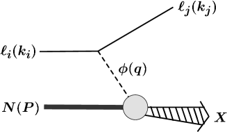
Figure 1: The CLFV lepton-nucleon scattering induced by $t$-channel exchange of the (pseudo-)scalar mediator. The initial and final lepton momenta are $k_{i}$ and $k_{j}$, respectively, and the nucleon momentum is $P$.

In Fig. 1 schematic diagram for the process $\ell_{i}N\to\ell_{j}X_{H}$ is shown, where initial lepton $\ell_{i}$ with a momentum $k_{i}$ and a nucleon $N$ with a momentum $P$ are scattered by exchanging the CLFV mediator $\phi$ with a momentum $q=k_{i}-k_{j}$. The final states are lepton $\ell_{j}$ with momentum $k_{j}$ and an arbitrary hadronic system $X_{H}$ which contains heavy quarks. The amplitude, where the CLFV mediator $\phi$ is exchanged in $t$-channel, is factorized into leptonic and hadronic amplitudes. The cross section $\sigma$ consists of the leptonic and hadronic parts, which are respectively denoted by $L_{\phi}$ and $F_{\phi}$, and is written in the following form:

$$\frac{d\sigma}{dxdy}\left(\ell_{i}N\to\ell_{j}X\right)=\frac{y\left|\rho_{qq}^{\phi}\right|^{2}L_{\phi}(Q^{2})\,F_{\phi}(x,Q^{2})}{16\pi\left(Q^{2}+m_{\phi}^{2}\right)^{2}},$$ (2)

where $m_{\phi}$ is a mediator mass, and the dimensionless variables $x,y$ are defined by

$$x=\frac{Q^{2}}{2P\cdot q},\hskip 28.45274pty=\frac{2P\cdot q}{2P\cdot k_{i}},$$ (3)

with $Q^{2}=-q^{2}=xy(s-m_{N}^{2})$. Here $s=(P+k_{i})^{2}$ is the collision energy squared of the initial lepton-nucleon system, and $m_{N}$ is the nucleon mass.

The leptonic part is given by

$$L_{\phi} = \big{(}|\rho_{ij}^{\phi}|^{2}+|\rho_{ji}^{\phi}|^{2}\big{)}\big{(}Q^{2}+m_{i}^{2}+m_{j}^{2}\big{)}+4\,{\rm Re}\left(\rho_{ij}^{\phi}\rho_{ji}^{\phi}\right)m_{i}m_{j},$$ (4)

with $m_{i(j)}$ being the initial (final) lepton mass, and the hadronic part is called structure function written in a convolution form as

$$F_{\phi}(x,Q^{2}) = \sum_{k}\int_{0}^{1}\frac{d\xi}{\xi}\ C_{\phi,\,k}\left(\frac{x}{\xi}\right)f_{k/N}(\xi,\mu_{f}^{2}),$$ (5)

where $k\in\{g,q,\bar{q}\}$ is a parton which contributes to the process $\phi k\rightarrow X$. The $C_{\phi,k}$ is a coefficient function calculable in perturbative QCD, while the parton distribution function (PDF) $f_{k/N}(x,\mu_{f}^{2})$ is a nonperturbative object which describes a probability of parton $k$ having momentum fraction $\xi$ inside the nucleon $N$ at a factorization scale $\mu_{f}^{2}$. The $\mu_{f}$-dependence is governed by renormalization group equation, so called Dokshitzer-Gribov-Lipatov-Altarelli-Parisi (DGLAP) equation Gribov and Lipatov (1972); Altarelli and Parisi (1977) :

$$\mu_{f}^{2}\frac{\partial~{}}{\partial\mu_{f}^{2}}f_{k/N}(\xi,\mu_{f}^{2}) = \sum_{l}\frac{\alpha_{s}(\mu_{f}^{2})}{2\pi}\int_{\xi}^{1}\frac{d\eta}{\eta}{\cal P}_{kl}\left(\frac{\xi}{\eta}\right)f_{l/N}(\xi,\mu_{f}^{2})+{\cal O}(\alpha_{s}^{2}),$$ (6)

where $l$ runs over possible quark flavors and gluon, and ${\cal P}_{kl}$ is a splitting function at one-loop level. Conventionally the factorization scale is chosen as $\mu_{f}^{2}\sim Q^{2}$ to be the same order as the hard scale in the process. For the heavy quark production, there are two hard scales $Q^{2},m_{q}^{2}$ in the process, and we will adopt a more refined scale setting (see Eq. (26)).

II.2 Cross sections and distribution

In theory discussion it is sometimes convenient to use $x,Q^{2}$ as independent variables instead of $x,y$. The conversion formula is given by

$$\frac{d^{2}\sigma}{dxdQ^{2}}(\ell_{i}N\to\ell_{j}X) = \left(\frac{1}{xs}\right)\frac{d^{2}\sigma}{dxdy}(\ell_{i}N\to\ell_{j}X).$$ (7)

Integrated over $x$ one obtains the differential cross section $d\sigma/dQ^{2}$ as

$$\frac{d\sigma}{dQ^{2}} = \frac{|\rho_{qq}^{\phi}|^{2}}{16\pi s^{2}}\frac{Q^{2}L_{\phi}(Q^{2})M_{\phi}(s,Q^{2})}{(Q^{2}+m_{\phi}^{2})^{2}},$$ (8)

where $M_{\phi}$ is the second inverse moment of the structure function defined by

$$M_{\phi}(s,Q^{2}) \equiv \int_{x_{\rm min}(s,Q^{2})}^{x_{\rm max}(Q^{2})}x^{-2}\,F_{\phi}(x,Q^{2})dx.$$ (9)

The integration region $[x_{\rm min}(s,Q^{2}),x_{\rm max}(Q^{2})]$ depends on partonic processes, and the $x_{\rm min}(s,Q^{2})$ depends on $s$ (see (58)), which introduces the collision energy dependence in the inverse moment. A derivation of the physical region for the CLFV DIS is given in the Appendix.

As a direct observable in collider experiments, we study the momentum distribution of the final lepton. To make our discussion concrete we give a cross section formula for $eN\to\tau X$ for fixed target experiment where the initial nucleon is at the rest. The initial nucleon and electron momenta are parametrized by $k_{e}=(E_{e},0,0,E_{e})$ and $P=(m_{N},0,0,0)$, respectively. Here we ignored the electron mass, and the nucleon mass is set to be $m_{N}=938\,{\rm MeV}$. The electron beam energy $E_{e}$ is related to the collision energy by $E_{e}=\sqrt{(s-m_{N}^{2})/2m_{N}}$. The final $\tau$-momentum at the nucleon rest frame is parametrized as $k_{\tau}=\left(E_{\tau},p_{T},0,p_{Z}\right)$ where $p_{T},p_{Z}$ are related to the dimensionless parameters $x,y$ as

$$p_{Z}=(1-y)E_{e}-xym_{N}-\frac{m_{\tau}^{2}}{2E_{e}},\hskip 14.22636ptp_{T}=\sqrt{(1-y)^{2}E_{e}^{2}-m_{\tau}^{2}-p_{Z}^{2}},$$ (10)

with $E_{\tau}=(1-y)E_{e}$. Then the $\tau$-momentum distribution at the nucleon rest frame is given by

$$\frac{d^{\,2}\sigma}{dp_{T}\,dp_{Z}}(\ell_{i}N\to\ell_{j}X) = \bigg{[}\frac{2p_{T}}{E_{\tau}y(s-m_{N}^{2})}\bigg{]}\frac{d^{2}\sigma}{dxdy}(\ell_{i}N\to\ell_{j}X),$$ (11)

where a Jacobian factor is multiplied in the right-hand side of Eq. (11) to convert the independent variables from $(x,y)$ to $(p_{T},p_{Z})$.

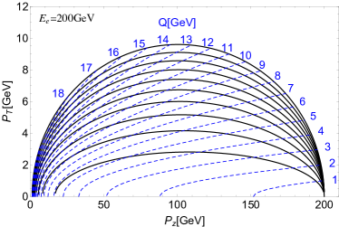
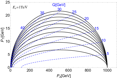
Figure 2: The physical region of the $\tau$-momentum for the process $eN\to\tau X$ in a fixed target experiment. The electron beam energy is $E_{e}=200\,{\rm GeV}$(left panel)/$1\,{\rm TeV}$(right panel). The contour lines of fixed $x$ (black lines) and fixed $Q$ (dashed blue lines) are plotted in the momentum space $(p_{z},p_{T})$.

In Fig. 2 the physical region of the $\tau$-momentum $(p_{Z},p_{T})$ is plotted for the beam energies $E_{e}=200\,{\rm GeV}$ and $1\,{\rm TeV}$ respectively in the left and right panels. The black lines are the contours for $x=0.1,0.2,\cdots,1.0$ from smaller to larger arcs, and the blue dashed lines are the contours for $Q$ values indicated in the plots. For CLFV signal searches in the fixed target experiments it is of great importance to have a reliable theory prediction that covers all the physical regions of Fig. 2.

II.3 Heavy quark contribution to structure function

In the following, we consider the heavy quark production via the CLFV scalar and pseudoscalar interactions. To be concrete we assume that the heavy quark $q$ is bottom or charm quark, which is much heavier than the nucleon, and treat other lighter quarks as massless. Formulae derived here can be also applied to top quark, but the threshold of top quark pair production is too high, and we do not discuss its phenomenology in the present article. The heavy quark mass is so large that its intrinsic partonic content inside the nucleon is zero. Yet the heavy quark can be produced in pair with its anti-quark via a gluon splitting $g\to q\bar{q}$ and subsequently $q$ or $\bar{q}$ is scattered by $\phi=S,P$ via the quark-mediator interaction of ${\cal L}_{\phi}$. In Fig. 3 an example Feynman diagram is shown for such a process.

Figure 3: A Feynman diagram for the heavy quark pair production in the CLFV lepton-nucleon scattering.

The corresponding hadronic part $F_{\phi}$ which contributes to the $\ell_{i}N\to\ell_{j}q\bar{q}X$ is given by

$$F_{\phi}^{{\rm M}}(x,Q^{2}) = \int_{0}^{1}\frac{d\xi}{\xi}\ C_{\phi,g}^{{\rm M}}\left(\frac{x}{\xi},\frac{Q^{2}}{m_{q}^{2}}\right)f_{g/N}(\xi,\mu_{f}^{2}),$$ (12)

where $C_{\phi,g}^{{\rm M}}$ is a heavy quark contribution to the coefficient function. The superscript M indicates that the quantity is computed in massive scheme, where the heavy quark mass is retained in the computation:

$$C_{S,g}^{{\rm M}}\left(\frac{x}{\xi},\frac{Q^{2}}{m_{q}^{2}}\right) = \frac{\alpha_{s}}{2\pi}\frac{T_{F}}{(Q^{2}+w^{2})^{2}}\Theta\left(w^{2}-4m_{q}^{2}\right)\bigg{\{}2Kw^{2}(Q^{2}+4m_{q}^{2})$$ (13)

$$\hskip 28.45274pt+\bigg{[}Q^{2}(Q^{2}+4m_{q}^{2})+(w^{2}-4m_{q}^{2})^{2}\bigg{]}\ln\frac{1+K}{1-K}\bigg{\}},$$

$$C_{P,g}^{{\rm M}}\left(\frac{x}{\xi},\frac{Q^{2}}{m_{q}^{2}}\right) = \frac{\alpha_{s}}{2\pi}\frac{T_{F}}{(Q^{2}+w^{2})^{2}}\Theta\left(w^{2}-4m_{q}^{2}\right)\bigg{\{}2Kw^{2}Q^{2}$$ (14)

$$\hskip 28.45274pt+\bigg{[}Q^{2}(Q^{2}+4m_{q}^{2})+w^{4}\bigg{]}\ln\frac{1+K}{1-K}\bigg{\}},$$

with $T_{F}=1/2$ and $\Theta(x)$ being the Heaviside step function. The $K=\sqrt{1-4m_{q}^{2}/w^{2}}$ is the speed of the heavy quark in the center-of-mass frame of the produced heavy quark pair with $w^{2}=(q+\xi P)^{2}=Q^{2}(\xi/x-1)$ being the invariant mass of $q\bar{q}$. Thus, the step function can be rewritten as $\Theta(w^{2}-4m_{q}^{2})=\Theta\left(\xi-\chi\right)$ with

$$\chi\equiv\left(1+\frac{4m_{q}^{2}}{Q^{2}}\right)x.$$ (15)

The appearance of $\chi$, not $x$, is an important mass effect due to the threshold of pair production of $q\bar{q}$. This leads $\chi$-rescaling prescription Tung et al. (2002); Kretzer et al. (2004) based on an idea of so-called slow-rescaling Barnett (1976), which will be discussed later.

II.4 SACOT scheme

(a)                    (b)  

Figure 4: Feynman diagrams for (a) the heavy quark pair production in scalar-gluon fusion, and (b) heavy quark excitation.

In Eqs.(13) and (14), the heavy quark contribution to the coefficient function is calculated retaining the heavy quark mass, which corresponds to the heavy quark pair production in scalar-gluon fusion (a) in Fig. 4, and its behavior around the threshold $w^{2}\sim 4m_{q}^{2}$ is correctly described order by order in perturbative expansion of $\alpha_{s}$. However when $Q^{2}\gg m_{q}^{2}$ there appears a large logarithm $\ln(Q^{2}/m_{q}^{2})$ in $C_{\phi,g}^{{\rm M}}$, and its appearance deteriorates the perturbative computation for $C_{\phi,g}^{{\rm M}}$. It can be seen by expanding $C_{\phi,g}^{{\rm M}}$ in the limit $(m_{q}^{2}/Q^{2})\to 0$:

$$C_{\phi,g}^{{\rm M}} \approx \int_{0}^{1}\frac{d\eta}{\eta}\bigg{[}C_{\phi,q}^{{\rm ZM}}\left(\frac{x}{\eta}\right)+C_{\phi,\bar{q}}^{{\rm ZM}}\left(\frac{x}{\eta}\right)\bigg{]}\,\Theta(\xi-\eta)\bigg{[}\left(\frac{\alpha_{s}}{2\pi}\right){\cal P}_{qg}\left(\frac{\eta}{\xi}\right)\ln\left(\frac{Q^{2}}{m_{q}^{2}}\right)\bigg{]},$$ (16)

where ${\cal P}_{qg}(z)=T_{F}\big{[}z^{2}+(1-z)^{2}\big{]}$ is a gluon-quark splitting function, and $C_{\phi,q}^{{\rm ZM}}(x),C_{\phi,\bar{q}}^{{\rm ZM}}(x)$ are single heavy quark contributions to the coefficient function in the massless limit, corresponding to the heavy quark excitation diagram (b) in Fig. 4:

$$C_{\phi,q}^{{\rm ZM}}\left(x\right)=C_{\phi,\bar{q}}^{{\rm ZM}}\left(x\right)=\frac{1}{2}\delta\left(1-x\right).$$ (17)

Therefore the high-energy limit of the structure function can be written as

$$F_{\rm\phi}^{{\rm M0}}(x,Q^{2}) = \int_{0}^{1}\frac{d\eta}{\eta}\ 2C_{\phi,q}^{{\rm ZM}}\left(\frac{x}{\eta}\right)\frac{\alpha_{s}}{2\pi}\ln\left(\frac{\mu_{f}^{2}}{m_{q}^{2}}\right)\int_{\eta}^{1}\frac{d\xi}{\xi}{\cal P}_{qg}\left(\frac{\eta}{\xi}\right)f_{g/N}(\xi,\mu_{f}^{2})$$ (18)

where the superscript M0 denotes the leading contribution in the massless limit of the massive scheme structure function. Namely the $F_{\phi}^{{\rm M0}}$ contains the mass singularity of the massive structure function, and $(F_{\phi}^{{\rm M}}-F_{\phi}^{{\rm M0}})$ is finite in the massless limit. Here, the original collinear logarithm existing in Eq. (16) is separated as $\alpha_{s}\ln(Q^{2}/m_{q}^{2})=\alpha_{s}\ln(Q^{2}/\mu_{f}^{2})+\alpha_{s}\ln(\mu_{f}^{2}/m_{q}^{2})$, and the mass singularity $\alpha_{s}\ln(\mu_{f}^{2}/m_{q}^{2})$ is absorbed in Eq. (18).

The relation between the high-energy limit of the massive quark contribution and the $F_{\phi}^{{\rm M0}}$ structure function is nothing but the factorization theorem Collins (1998) of collinear singularities for the QCD structure function, which can be utilized to resum the large collinear logarithms to all orders in $\alpha_{s}$ to make the structure functions stable at high energy. The extracted collinear logarithm $\alpha_{s}\ln(\mu_{f}^{2}/m_{q}^{2})$ has a form, that can be resummed to all orders in $\alpha_{s}$ by means of the standard DGLAP evolution equation, leading to zero-mass (ZM) scheme structure function $F_{\phi}^{{\rm ZM}}$:

$$F_{\phi}^{{\rm ZM}}(x,Q^{2}) = \int_{0}^{1}\frac{d\eta}{\eta}\ 2C_{\phi,q}^{{\rm ZM}}\left(\frac{x}{\eta}\right)\big{[}f_{q/N}(\eta,\mu_{f}^{2})+f_{\bar{q}/N}(\eta,\mu_{f}^{2})\big{]}$$ (19)

$$= \frac{1}{2}\big{[}f_{q/N}(x,\mu_{f}^{2})+f_{\bar{q}/N}(x,\mu_{f}^{2})\big{]}.$$

The heavy quark PDFs $f_{q/N}$ and $f_{\bar{q}/N}$ introduced in Eq. (19) are generated by the gluon splitting into $q\bar{q}$ through the DGLAP evolution equation, and thus reduces to Eq. (18) at the leading order in $\alpha_{s}$ expansion:

$$f_{q/N}(x,\mu_{f}^{2}) = \frac{\alpha_{s}}{2\pi}\ln\left(\frac{\mu_{f}^{2}}{m_{q}^{2}}\right)\int_{x}^{1}\frac{d\xi}{\xi}\ {\cal P}_{qg}\left(\frac{x}{\xi}\right)f_{g/N}(\xi,\mu_{f}^{2})+{\cal O}(\alpha_{s}^{2}).$$ (20)

So far we have defined three types of structure function $F_{\phi}^{\rm M},F_{\phi}^{{\rm M0}}$ and $F_{\phi}^{{\rm ZM}}$. The M-scheme structure function is reliable in low-$Q^{2}$ region but unreliable in the high-$Q^{2}$ region due to the mass singularity, while the ZM scheme structure function is reliable in the high-$Q^{2}$ region but unreliable in the low-$Q^{2}$ region. Therefore these two are complementary to each other. According to these observations, a scheme for the structure function was constructed, which includes heavy quark mass effects near $q\bar{q}$ threshold region and also the large logarithm resummation making the structure function stable even at high-$Q^{2}$ region. The result is a new structure function which consists of three terms as

$$F_{\phi}^{\rm SACOT}\left(x,Q^{2}\right) = F_{\phi}^{\rm M}\left(x,Q^{2}\right)+F_{\phi}^{{\rm ZM}}\left(x,Q^{2}\right)-F_{\phi}^{\rm sub}(x,Q^{2}).$$ (21)

Here the second and third terms are computed by setting heavy quark masses to zero, and this is called Simplified ACOT (SACOT) scheme Krämer et al. (2000); Aivazis et al. (1994b). The first term $F_{\phi}^{\rm M}$ is the contribution of a heavy quark pair to the structure function where the heavy quarks $q,\bar{q}$ are massive and produced in the scalar-gluon fusion. The second term $F_{\phi}^{{\rm ZM}}$ is the contribution of heavy quark excitations, and plays a role to resum the large-collinear logarithm $\ln(Q^{2}/m_{q}^{2})$ to all orders in $\alpha_{s}$ by use of the heavy quark and anti-quark PDFs $\{f_{q/N},f_{\bar{q}/N}\}$. By the construction of $F_{\phi}^{{\rm ZM}}$, there is a double counting of large-logarithm between $F_{\phi}^{\rm M}$ and $F_{\phi}^{{\rm ZM}}$, and this double counting effect should be subtracted by the last term:

$$F_{\phi}^{\rm sub}(x,Q^{2}) = F_{\phi}^{{\rm M0}}(x,Q^{2}).$$ (22)

The physical picture of the SACOT scheme is as follows: the first term $F_{\phi}^{\rm M}$ contains all the mass effects order by order in the expansion of powers of $\alpha_{s}$, and the second term $F_{\phi}^{\rm ZM}$ adds the large logarithmic corrections of $(\alpha_{s}\ln(Q^{2}/m_{q}^{2}))^{n}$ for $n=1,\cdots,\infty$ to improve the high-$Q^{2}$ behavior avoiding the double counting by the last term $F_{\phi}^{\rm sub}$.

II.5 Improvements for threshold behavior

Although we are working on the leading order formulation for the heavy quark structure function, there are a number of important effects, which can be incorporated in the present computation, on the threshold behavior of the structure functions. We take into account such improvements here.

The first such effect is one by so-called $\chi$-rescaling prescriptionTung et al. (2002); Kretzer et al. (2004). The $\chi$-rescaling prescription aims to incorporate threshold kinematics of the heavy quark production into the massless structure function (ZM) and the massless limit (M0) of the massive structure function using $\chi(x,Q^{2})$ introduced in Eq.(15) instead of $x$ variable. This defines structure functions in ZM-$\chi$ and M0-$\chi$ schemes:

$$F_{\phi}^{{\rm ZM\mathchar 45\relax\chi}}(x,Q^{2}) = \frac{1}{2}\big{[}f_{q/N}(\chi(x,Q^{2}),\mu_{f}^{2})+f_{\bar{q}/N}(\chi(x,Q^{2}),\mu_{f}^{2})\big{]},$$ (23)

$$F_{\rm\phi}^{{\rm M0\mathchar 45\relax\chi}}(x,Q^{2}) = \frac{\alpha_{s}}{2\pi}\ln\left(\frac{\mu_{f}^{2}}{m_{q}^{2}}\right)\int_{\chi(x,Q^{2})}^{1}\frac{d\xi}{\xi}{\cal P}_{qg}\left(\frac{\chi(x,Q^{2})}{\xi}\right)f_{g/N}(\xi,\mu_{f}^{2}).$$ (24)

The subtraction term with $\chi$-rescaling is similarly defined by $F_{\phi}^{{\rm sub\mathchar 45\relax\chi}}(x,Q^{2})=F_{\phi}^{{\rm M0\mathchar 45\relax\chi}}(x,Q^{2})$. With these structure functions SACOT-$\chi$ scheme is also defined as

$$F_{\phi}^{{\rm SACOT\mathchar 45\relax\chi}}(x,Q^{2}) \equiv F_{\phi}^{\rm M}\left(x,Q^{2}\right)+\big{[}F_{\phi}^{{\rm ZM\mathchar 45\relax\chi}}\left(x,Q^{2}\right)-F_{\phi}^{{\rm sub\mathchar 45\relax\chi}}(x,Q^{2})\big{]}.$$ (25)

The second improvement is a choice of the factorization scale $\mu_{f}^{2}$. In the traditional DIS analysis the scale choice $\mu_{f}^{2}=Q^{2}$ is commonly used assuming $Q^{2}\gg m_{q}^{2}$. However we are interested in not only high-$Q^{2}$ but also the threshold region of the heavy quark production, especially the contribution from the gluon fusion of Fig. 3, for which $Q^{2}$ can be the same order with $m_{q}^{2}$ or even smaller than $m_{q}^{2}$. For such a case, the scale choice $\mu_{f}^{2}=Q^{2}$ is not suitable, and one needs to take a proper physical scale of the process. To ensure that the factorization scale does not become too low, we take the scale as $\mu_{f}^{2}=\mu_{Q}^{2}$ with

$$\mu_{Q}^{2} = Q^{2}\,\big{[}c\,(1-z_{m})^{n}\,\Theta(1-z_{m})+z_{m}\big{]},$$ (26)

where $z_{m}=m_{q}^{2}/Q^{2}$, $n=2$ and $c=0.5$ are chosen following Ref.Aivazis et al. (1994b).

The SACOT-$\chi$ structure function interpolates between massive $F_{\phi}^{{\rm M}}$ and massless $F_{\phi}^{{\rm ZM\mathchar 45\relax\chi}}$ structure functions. Ideally $F_{\phi}^{{\rm SACOT\mathchar 45\relax\chi}}$ is supposed to reduce to the massive one in the low-$Q^{2}$ region, while in the high-$Q^{2}$ region to the massless one. This expectation holds parametrically at each order in expansion in powers of $\alpha_{s}$, but numerically it can happen that the $F_{\phi}^{{\rm SACOT\mathchar 45\relax\chi}}$ does not converge well to $F_{\phi}^{{\rm M}}$ near the heavy quark threshold $Q^{2}\sim m_{q}^{2}$. If the cancellation between $F_{\phi}^{{\rm ZM\mathchar 45\relax\chi}}$ and $F_{\phi}^{{\rm sub\mathchar 45\relax\chi}}$ in low-$Q^{2}$ region is not effective, it must be due to unsuppressed higher-order terms in powers of $\alpha_{s}$ resummed into $F_{\phi}^{{\rm ZM\mathchar 45\relax\chi}}$. Namely the terms $F_{\phi}^{{\rm ZM\mathchar 45\relax\chi}}-F_{\phi}^{{\rm sub\mathchar 45\relax\chi}}={\cal O}(\alpha_{s}^{k}L^{k})~{}(k\geq 2)$ are too large in the region where the massless approximation is not trustable. Easy solution to avoid this trouble is to suppress the $F_{\phi}^{{\rm ZM\mathchar 45\relax\chi}}-F_{\phi}^{{\rm sub\mathchar 45\relax\chi}}$ in low-$Q^{2}$ region by hand. Thus we define improved structure functions for ZM-$\chi$ and M0-$\chi$ schemes:

$$F_{\phi,\rm thr}^{{\rm ZM\mathchar 45\relax\chi}}\left(x,Q^{2}\right) = F_{\phi}^{{\rm ZM\mathchar 45\relax\chi}}\left(x,Q^{2}\right)S_{\rm thr}(m_{q}^{2}/Q^{2}),$$ (27)

$$F_{\phi,\rm thr}^{{\rm M0\mathchar 45\relax\chi}}\left(x,Q^{2}\right) = F_{\phi,\rm thr}^{\rm sub\chi}\left(x,Q^{2}\right)=F_{\phi}^{{\rm M0\mathchar 45\relax\chi}}(x,Q^{2})S_{\rm thr}(m_{q}^{2}/Q^{2}),$$ (28)

where $S_{\rm thr}(m_{q}^{2}/Q^{2})$ is a function which suppress the structure functions in ZM-$\chi$ and M0-$\chi$ schemes forcing them to smoothly match with correct threshold behavior. The functional form of $S_{\rm thr}(z)$ is somewhat arbitrary but the only requirement is $S_{\rm thr}(z)\stackrel{{\scriptstyle z\to 0}}{{\to}}1$ for the large-logarithm resummation for high $Q^{2}$. For simplicity we choose

$$S_{\rm thr}(z)=\left(1-z\right)^{2}~{}\Theta\left(1-z\right),$$ (29)

in the same form introduced in Ref. Forte et al. (2010). Taking all the improvements we define the SACOT-$\chi$(thr) structure function by

$$F_{\phi,{\rm thr}}^{{\rm SACOT\mathchar 45\relax\chi}}(x,Q^{2}) \equiv F_{\phi}^{{\rm M}}\left(x,Q^{2}\right)+\big{[}F_{\phi,\rm thr}^{{\rm ZM\mathchar 45\relax\chi}}\left(x,Q^{2}\right)-F_{\phi,\rm thr}^{{\rm sub\mathchar 45\relax\chi}}(x,Q^{2})\big{]}.$$ (30)

The combination $\big{[}F_{\phi,\rm thr}^{{\rm ZM\mathchar 45\relax\chi}}-F_{\phi,\rm thr}^{{\rm sub\mathchar 45\relax\chi}}\big{]}$ ensures that the SACOT-$\chi$(thr) structure function reduces to massive one near heavy quark threshold. For the SACOT-$\chi$(thr) scheme, we always adopt the scale setting $\mu_{f}^{2}=\mu_{Q}^{2}$ and the threshold factor $S_{\rm thr}(m_{q}^{2}/Q^{2})$.

III Numerical analysis: Structure functions

We analyze the structure functions for the scalar interaction, i.e. $\phi=S$. The pseudoscalar case ($\phi=P$) is much the same as the scalar case, and we refrain from showing the numerical results for the pseudoscalar case. In the present article we use CT14 LO PDFs Dulat et al. (2016), and present the numerics for the proton with $m_{N}=938\,{\rm MeV}$ as a target nucleon. The scale choice $\mu_{f}^{2}=\mu_{Q}^{2}$ is adopted for all the structure functions.

III.1 Effect of $\chi$-rescaling on the structure functions

Figure 5: The structure functions $F_{\phi}$ computed in the ZM-$\chi$, ZM-$x$, M0-$\chi$, and M0-$x$ schemes are plotted as functions of $Q$ for $x=0.3$ and $x=0.03$ in the left and right columns, respectively. The upper and lower rows show the contributions of the bottom ($q=b$) and charm ($q=c)$ quarks, respectively.

Let us first discuss the importance of $\chi$-rescaling for the structure functions in the ZM and M0 schemes in low-$Q^{2}$ region. For the QCD structure functions effects of $\chi$-rescaling are discussed in Refs. Tung et al. (2002); Kretzer et al. (2004); Stavreva et al. (2012). To make the difference explicit between the structure functions using $x$ and $\chi$ variables, we introduce the following notations: $F_{\phi}^{{\rm ZM\mathchar 45\relax}x}(=F_{\phi}^{{\rm ZM}}),F_{\phi}^{{\rm M0\mathchar 45\relax}x}(=F_{\phi}^{{\rm M0}})$. Hereafter we call them $x$-scheme structure functions when the distinction is necessary. The ZM and M0 structure functions ($x$-scheme) in Eqs.(18) and (19) do not contain any information on the heavy quark threshold. Thus there is no reason to trust $F_{\phi}^{{\rm ZM\mathchar 45\relax}x},F_{\phi}^{{\rm M0\mathchar 45\relax}x}$ near the heavy quark threshold, but it is still expected to have an improvement on the threshold behavior near $Q^{2}=m_{q}^{2}$ by the $\chi$-rescaling. In Fig. 5 the ZM and M0 structure functions are plotted as functions of $Q$. The structure functions for $x=0.3$ and $0.03$ are shown in the left and right columns, and those for bottom and charm quarks are shown in the upper and lower rows. The solid lines represent the ZM-$\chi$ and M0-$\chi$ structure functions, and the dot-dashed lines represent the corresponding $x$-scheme structure functions. One can see that the effect of $\chi$-rescaling is huge and plays an essential role for the threshold suppression near $Q\sim m_{q}$ ($m_{b}=4.75\,{\rm GeV}$ for bottom quark and $m_{c}=1.3\,{\rm GeV}$ for charm quark). The $x$-scheme structure functions are unrealistically large for $Q\sim m_{q}$, and it is remarkable that the $\chi$-rescaling improves the unphysical behavior of the massless structure functions nicely. The effect of $\chi$-rescaling is decreasing in high-$Q^{2}$ region, and the difference between the use of $x$ and $\chi$-rescaling is negligible at $Q=100\,{\rm GeV}$ ($Q=50\,{\rm GeV}$) for bottom (charm) quark. We conclude that the $\chi$-rescaling is effective only in the low-$Q^{2}$ region of $Q\leq 100\,{\rm GeV}~{}(Q\leq 50\,{\rm GeV})$ for bottom (charm) quark.

III.2 Massive vs. zero-mass schemes, and SACOT scheme

Figure 6: The structure functions $F_{\phi}$ in the ZM-$\chi$, M0-$\chi$, M, and SACOT-$\chi$(thr) schemes are plotted as functions of $Q$ for $x=0.3$ and $x=0.03$ in the left and right columns, respectively. The upper and lower rows show the contributions of bottom ($q=b$) and charm ($q=c$) quarks, respectively.

Figure 7: Same as Fig. 6 but for low-$Q^{2}$ region: $x=0.3$ (left column) and $x=0.03$ (right column) for bottom ($q=b)$ and charm ($q=c$) quarks in the two rows.

Here we will compare the structure functions in M, ZM-$\chi$(thr), and SACOT-$\chi$(thr) schemes (for the last two schemes $\chi$-rescaling and the threshold factor are adopted). In Fig. 6 the heavy quark contribution to the structure functions are plotted as functions of $Q$ (up to $Q=300\,{\rm GeV}$) for $x=0.3$ and $x=0.03$. For $x=0.3$ it is seen that the curves for SACOT-$\chi$(thr) and ZM-$\chi$(thr) are broadly similar to each other for bottom and charm quarks, and their values are much larger than the massive scheme result. The difference between the curves of the ZM-$\chi$(thr) and SACOT-$\chi$(thr) schemes is explained by the difference between the M and M0-$\chi$ schemes because $(F_{\phi,\rm thr}^{{\rm SACOT\mathchar 45\relax\chi}}-F_{\phi,\rm thr}^{{\rm ZM\mathchar 45\relax\chi}})=(F_{\phi}^{\rm M}-F_{\phi,\rm thr}^{{\rm M0\mathchar 45\relax\chi}})$. Remember that $F_{\phi,\rm thr}^{{\rm M0\mathchar 45\relax\chi}}$   is the subtraction term of the SACOT-$\chi$(thr) scheme. For $x=0.03$ this agreement between the SACOT-$\chi$(thr) and ZM-$\chi$(thr) schemes becomes tighter, because $(F_{\phi}^{{\rm M}}-F_{\phi,\rm thr}^{{\rm sub\mathchar 45\relax\chi}})_{x=0.03}\simeq 0$. It should be noted that the structure functions for $x=0.03$ are more than two orders of magnitude larger than those of $x=0.3$.

The same plots as Fig. 6, focusing on the range below $Q=30\,{\rm GeV}$, are shown in Fig. 7. It will be seen later that the contributions of the structure functions to the CLFV DIS cross section for $E_{e}\leq 1\,{\rm TeV}$ are dominated by the $Q$ values of this range. Therefore Fig. 7 is more relevant than Fig. 6 for the fixed target experiments at present and in near future. For bottom quark, the M scheme structure function is closer to the SACOT-$\chi$(thr) scheme than ZM-$\chi$(thr) for $x=0.03$. For $x=0.3$ both the curves of M and ZM-$\chi$(thr) are away from the SACOT-$\chi$(thr) but their magnitudes are less than percent level compared to those at $x=0.03$. For charm quark at $x=0.03$, the M scheme structure function is closer to the SACOT-$\chi$(thr) for very low $Q$. For $Q\geq 8.6\,{\rm GeV}$ the ZM-$\chi$(thr) scheme becomes closer to SACOT-$\chi$(thr) especially for the large-$Q^{2}$ region. For charm quark at $x=0.3$, the magnitudes of the structure functions are less than a percent level compared to those at $x=0.03$.

III.3 Threshold factor

In Figs. 6 and 7 the threshold factor $S_{\rm thr}$ had been taken into account for the structure functions $F_{\phi}^{{\rm SACOT\mathchar 45\relax\chi}}$, $F_{\phi}^{{\rm ZM\mathchar 45\relax\chi}}$, and $F_{\phi}^{{\rm M0\mathchar 45\relax\chi}}$. The effect of the threshold factor is limited in low-$Q^{2}$ region: $S_{\rm thr}(m_{b}^{2}/Q^{2})=0.60,0.89,0.95$ for $Q=10,20,30\,{\rm GeV}$ for bottom quark, and $S_{\rm thr}(m_{c}^{2}/Q^{2})=0.87,0.97,0.99$ for $Q=5,10,15\,{\rm GeV}$ for charm quark. These values give about $40\%,11\%,5\%$ suppressions for the structure functions $F_{\phi,\rm thr}^{{\rm ZM\mathchar 45\relax\chi}},F_{\phi,\rm thr}^{{\rm M0\mathchar 45\relax\chi}}$ of bottom quark at $Q=10,20,30\,{\rm GeV}$ compared to those without the threshold factor, and about $13\%,3\%,1\%$ suppressions for the charm quark case at $Q=5,10,15\,{\rm GeV}$. For the SACOT-$\chi$(thr) scheme the relative size of $(F_{\phi,\rm thr}^{{\rm M0\mathchar 45\relax\chi}}-F_{\phi,\rm thr}^{{\rm ZM\mathchar 45\relax\chi}})=S_{\rm thr}(m_{q}^{2}/Q^{2})(F_{\phi}^{{\rm M0\mathchar 45\relax\chi}}-F_{\phi}^{{\rm ZM\mathchar 45\relax\chi}})$ to $F_{\phi}^{{\rm M}}$ determines the effect of $S_{\rm thr}$:

$$\frac{F_{\phi,{\rm thr},b}^{{\rm SACOT\mathchar 45\relax\chi}}}{F_{\phi,b}^{{\rm SACOT\mathchar 45\relax\chi}}}=\bigg{\{}\begin{array}[]{ll}0.94,~{}0.97,~{}0.98&(x=0.3)\\ 0.99,~{}0.99,~{}1.0&(x=0.03)\end{array}~{}~{}~{}\mbox{for}~{}Q=10,20,30\,{\rm GeV},$$ (33)

for bottom quark, and

$$\frac{F_{\phi,{\rm thr},c}^{{\rm SACOT\mathchar 45\relax\chi}}}{F_{\phi,c}^{{\rm SACOT\mathchar 45\relax\chi}}}=\bigg{\{}\begin{array}[]{ll}0.95,~{}0.98,~{}0.99&(x=0.3)\\ 0.99,~{}1.0,~{}1.0&(x=0.03)\end{array}~{}~{}~{}\mbox{for}~{}Q=5,10,15\,{\rm GeV},$$ (36)

for charm quark. It is understood that a major part of the threshold suppression is already taken care by the $\chi$-rescaling, and the effect of $S_{\rm thr}$ became minor for the structure function in the SACOT-$\chi$(thr) scheme.

IV Numerical Analysis: Cross sections

In this section, we investigate how effective the SACOT-$\chi$ scheme and the others are for the description of CLFV process associated with the heavy quark pair productions. As a continuation of the previous section only the scalar case ($\phi=S$) will be studied. As is explained in the previous section, the structure functions are functions of $x$ and $Q^{2}$, and each scheme of the structure functions has validity regions for a specific $Q^{2}$ range. However our concerns are the total cross sections $\sigma$ and differential distributions $d\sigma/d\bm{p}_{\tau}$ of the final $\tau$-momentum. There arises a question of which scheme is the most relevant, and which scheme is the most effective for the description of the CLFV DIS in the full kinematical range of the cross section, which will be answered in this section.

For definiteness we take electron and tau lepton as initial and final leptons, respectively, namely $i=e$ and $j=\tau$. In the numerical analysis we ignore the electron mass, and take the following mass values:

$$m_{b}=4.75\,{\rm GeV},~{}m_{c}=1.3\,{\rm GeV},~{}m_{\tau}=1.78\,{\rm GeV}.$$ (37)

The CLFV couplings $\rho_{ij}^{\phi}$ and quark-mediator coupling $\rho_{qq}^{\phi}$ are a priori not known and we set their values as

$$|\rho^{\phi}_{qq}|^{2}=|\rho_{ij}^{\phi}|^{2}+|\rho_{ji}^{\phi}|^{2}=1.$$ (38)

These coupling constants determine the normalization of the CLFV cross section, and therefore our numerical results need to be multiplied by mode-dependent prefactors to match them with experimental values to be measured. For the choice of the factorization scale $\mu_{f}^{2}$ we adopt $\mu_{f}^{2}=\mu_{Q}^{2}$ defined in Eq. (26). In our numerical analysis, we have applied a kinematical cut of $Q\geq 1.3\,{\rm GeV}$ and $W\equiv\sqrt{(P+q)^{2}}\geq 1.4\,{\rm GeV}$ to ensure that the processes we are considering are in perturbative and deep-inelastic régime, though it turned out that the effect of the cut is tiny and numerically negligible for the CLFV DIS associated with the heavy quark pair productions.

IV.1 Zero-mass schemes

The ZM schemes are the most frequently used schemes for DIS involving heavy quarks as well as the light quarks. This is so even for the CLFV DIS associated with bottom and charm quark productions because of their computational simplicities. However, the use of massless approximation cannot be justified for low $Q^{2}$, and a reliable computational scheme should be the massive scheme there. Nevertheless, it is worthwhile to know limitations of the ZM schemes for the CLFV cross sections. Here we investigate the ZM-$x$ and ZM-$\chi$ schemes to clarify their applicability for the cross section in relatively low collision energies. As example cases, we simulate the cross section for $E_{e}=200\,{\rm GeV}$ and $E_{e}=1\,{\rm TeV}$. Here we do not include the threshold factor $S_{\rm thr}$ for the ZM schemes because it cuts away the low-$Q^{2}$ region and the difference between ZM-$x$ and ZM-$\chi$ are naturally suppressed.

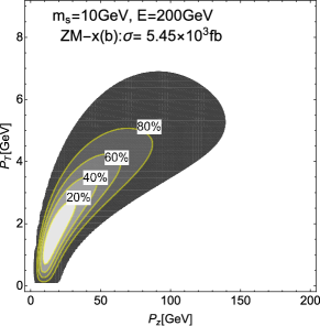
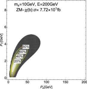
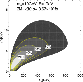
Figure 8: The $\tau$-momentum distributions Eq. (11) for the bottom quark production in the ZM-$x$(left column) and ZM-$\chi$ (right column) schemes. The distributions for the electron beam energies of $E_{e}=200\,{\rm GeV}$ (upper row) and $E_{e}=1\,{\rm TeV}$ (lower row) with scalar mass $m_{S}=10\,{\rm GeV}$ are shown.

In Fig. 8 we show the $\tau$-momentum distributions for the CLFV DIS associated with bottom quark production for $E_{e}=200\,{\rm GeV}$ and $E_{e}=1\,{\rm TeV}$ in the two rows. The scalar mass is set to $m_{S}=10\,{\rm GeV}$. The left and right columns show the distributions in the ZM-$x$ and ZM-$\chi$ schemes, respectively. The contour lines are labeled by percentages ($20\%,40\%,60\%,80\%$) of the cross section of the enclosed region normalized to their total cross section. The colored region contains $99\%$ of total events of the process. The value of the scalar mass $m_{S}$, the beam energy $E_{e}$, and the total cross section $\sigma$ are shown inside each panel. For $E_{e}=200\,{\rm GeV}$ the effect of $\chi$-rescaling is huge suppression for the overall normalization $\sigma$, and the physical regions of $\chi$-scheme distributions are shrunk into a smaller region than those of $x$-schemes. For $E_{e}=1\,{\rm TeV}$ the effect of $\chi$-rescaling is still large for the overall normalization but weak compared to the case of $E_{e}=200\,{\rm GeV}$. The ratio of the total cross section in $x$-scheme to that in $\chi$-scheme is $\sigma^{{\rm ZM\mathchar 45\relax}x}_{b}/\sigma^{{\rm ZM\mathchar 45\relax\chi}}_{b}\sim 70~{}(3.8)$ for $E_{e}=200\,{\rm GeV}~{}(1\,{\rm TeV})$. The large enhancements of the total cross sections in $x$-schemes hold even in the case of heavy scalar mass. For instance, taking $m_{S}=10^{5}\,{\rm GeV}$, the cross section ratio is $\sigma_{b}^{{\rm ZM\mathchar 45\relax}x}/\sigma_{b}^{{\rm ZM\mathchar 45\relax\chi}}\sim 73~{}(3.0)$ for $E_{e}=200\,{\rm GeV}~{}(1\,{\rm TeV})$ for the bottom quark production.

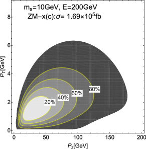
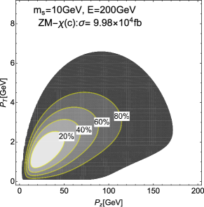
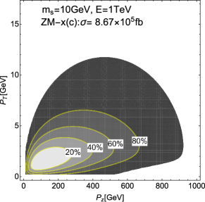
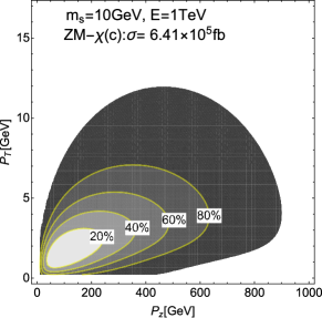
Figure 9: Same as Fig. 8, but heavy quark is charm quark ($q=c$): ZM-$x$ (left column) and ZM-$\chi$ (right column) for $E_{e}=200\,{\rm GeV}$ and $E_{e}=1\,{\rm GeV}$ in the two rows.

In Fig. 9 we show the $\tau$-momentum distributions for $m_{S}=10\,{\rm GeV}$ in the case of charm quark production. Comparing the $x$ and $\chi$ schemes, the shapes of the contour lines look quite similar to each other, but the effect of $\chi$-rescaling is still sizable for the normalization of total cross sections. The ratio is $\sigma_{c}^{{\rm ZM\mathchar 45\relax}x}/\sigma_{c}^{{\rm ZM\mathchar 45\relax\chi}}\sim 1.7~{}(1.4)$ for $E_{e}=200\,{\rm GeV}~{}(1\,{\rm TeV})$. This value is not changed much even for the heavy scalar case. For instance, taking $m_{S}=10^{5}\,{\rm GeV}$, the ratio is $\sigma_{c}^{{\rm ZM\mathchar 45\relax}x}/\sigma_{c}^{{\rm ZM\mathchar 45\relax\chi}}\sim 1.6~{}(1.2)$ for $E_{e}=200\,{\rm GeV}~{}(1\,{\rm TeV})$.

Figure 10: The cross sections for the CLFV DIS in the M, ZM-$x$, and ZM-$\chi$ schemes normalized to the SACOT-$\chi$(thr). The scale of the upper horizontal axis in each panel shows the beam energy in the fixed target experiments. The results for bottom ($q=b$) and charm ($q=c$) quarks are shown in the upper and lower rows, and the results for the scalar masses $m_{S}=10\,{\rm GeV}$ and $m_{S}=10^{5}\,{\rm GeV}$ are shown in the left and right columns.

In Fig. 10 the total cross sections associated with bottom and charm quark productions are plotted respectively in the upper and lower rows, where each cross section is normalized to the value of SACOT-$\chi$(thr). The left and right columns are two cases of scalar mass, $m_{S}=10\,{\rm GeV}$ and $10^{5}\,{\rm GeV}$, respectively. Numerical values of the cross sections are listed in Table 1. In the plots we observe the following:

• For the bottom quark production the curves of M scheme are close to the one of SACOT-$\chi$(thr), i.e. $\sigma_{b}^{\rm M}/\sigma_{{\rm thr},b}^{{\rm SACOT\mathchar 45\relax\chi}}\sim 1$. The cross section in the ZM-$\chi$ scheme for the small scalar mass $m_{S}=10\,{\rm GeV}$ is quite off from that of SACOT-$\chi$(thr) irrespective of the collision energy: $\sigma_{b}^{{\rm ZM\mathchar 45\relax\chi}}/\sigma_{{\rm thr},b}^{{\rm SACOT\mathchar 45\relax\chi}}\lesssim 0.5.$ For the case of the large scalar mass $m_{S}=10^{5}\,{\rm GeV}$, the ZM-$\chi$ and ZM-$x$ curves are gradually approaching to the SACOT-$\chi$ , and around $\sqrt{s}\sim 10^{3}\,{\rm GeV}$ they meet at one point. Notably, the curve of the ZM-$x$ scheme for the bottom production is far off from that of SACOT-$\chi$(thr) in low collision energy.

• Even for the charm quark production, inadequacy of the ZM-$x$ scheme in low collision energy is the same as the case of bottom quark, but the behaviors of the cross sections in the M and ZM-$\chi$ schemes are quite different. Specifics of the charm cross sections are as follows. For the small scalar mass $m_{S}=10\,{\rm GeV}$ the M scheme curve grows with $\sqrt{s}$ and overshoots the SACOT-$\chi$(thr) at $\sqrt{s}\sim 10^{2}\,{\rm GeV}$, while for the large scalar mass $m_{S}=10^{5}\,{\rm GeV}$ it is almost constant and small by a sizable amount compared to the SACOT-$\chi$(thr). For the large scalar mass, the value of the ZM-$\chi$ is close to the one of SACOT-$\chi$(thr) for arbitrary collision energy, and it is expected that charm quark can be treated as massless provided that the $\chi$-rescaling is adopted and the scalar mass is large enough. It will be shown in Fig. 17 that the scalar mass of $m_{S}\sim 50\,{\rm GeV}$ is large enough to validate the treatment of massless charm with $\chi$-rescaling adopted for it.

Table 1: The CLFV total cross sections associated with bottom and charm quark productions in ZM-$x$, ZM-$\chi$, and M schemes. The coupling constants are set to one by Eq. (38).

$m_{S}~{}[\rm{GeV}]$	$E_{e}~{}{\rm[GeV]}$	$\sigma_{b}^{{\rm ZM\mathchar 45\relax}x}~{}{\rm[fb]}$	$\sigma_{b}^{{\rm ZM\mathchar 45\relax\chi}}~{}{\rm[fb]}$	$\sigma_{b}^{\rm M}~{}{\rm[fb]}$
	$10^{2}$	$6.49\times 10^{2}$	$1.02\times 10^{-2}$	$2.08\times 10^{-1}$
	$10^{3}$	$8.67\times 10^{4}$	$2.28\times 10^{4}$	$4.93\times 10^{4}$
$10$	$10^{4}$	$7.84\times 10^{5}$	$3.72\times 10^{5}$	$7.32\times 10^{5}$
	$10^{5}$	$3.24\times 10^{6}$	$1.90\times 10^{6}$	$3.72\times 10^{6}$
	$10^{6}$	$9.12\times 10^{6}$	$5.87\times 10^{6}$	$1.18\times 10^{7}$
	$10^{7}$	$2.11\times 10^{7}$	$1.43\times 10^{7}$	$2.99\times 10^{7}$
	$10^{2}$	$1.51\times 10^{-13}$	$2.02\times 10^{-18}$	$3.17\times 10^{-17}$
	$10^{3}$	$5.64\times 10^{-11}$	$1.89\times 10^{-11}$	$2.23\times 10^{-11}$
$10^{5}$	$10^{4}$	$1.88\times 10^{-9}$	$1.41\times 10^{-9}$	$1.27\times 10^{-9}$
	$10^{5}$	$3.35\times 10^{-9}$	$3.10\times 10^{-8}$	$2.57\times 10^{-8}$
	$10^{6}$	$4.66\times 10^{-7}$	$4.57\times 10^{-7}$	$3.66\times 10^{-7}$
	$10^{6}$	$5.76\times 10^{-6}$	$5.73\times 10^{-6}$	$4.50\times 10^{-6}$
$m_{S}~{}[\rm{GeV}]$	$E_{e}~{}{\rm[GeV]}$	$\sigma_{c}^{{\rm ZM\mathchar 45\relax}x}~{}{\rm[fb]}$	$\sigma_{c}^{{\rm ZM\mathchar 45\relax\chi}}~{}{\rm[fb]}$	$\sigma_{c}^{\rm M}~{}{\rm[fb]}$
	$10^{2}$	$6.57\times 10^{4}$	$2.99\times 10^{4}$	$2.74\times 10^{4}$
	$10^{3}$	$8.67\times 10^{5}$	$6.41\times 10^{5}$	$6.59\times 10^{5}$
$10$	$10^{4}$	$4.10\times 10^{6}$	$3.46\times 10^{6}$	$4.15\times 10^{6}$
	$10^{5}$	$1.15\times 10^{7}$	$1.02\times 10^{7}$	$1.46\times 10^{7}$
	$10^{6}$	$2.45\times 10^{7}$	$2.24\times 10^{7}$	$3.83\times 10^{7}$
	$10^{7}$	$4.68\times 10^{7}$	$4.33\times 10^{7}$	$8.68\times 10^{7}$
	$10^{2}$	$1.00\times 10^{-11}$	$4.75\times 10^{-12}$	$3.86\times 10^{-12}$
	$10^{3}$	$3.03\times 10^{-10}$	$2.55\times 10^{-10}$	$1.93\times 10^{-10}$
$10^{5}$	$10^{4}$	$4.92\times 10^{-9}$	$4.70\times 10^{-9}$	$3.51\times 10^{-9}$
	$10^{5}$	$6.37\times 10^{-8}$	$6.31\times 10^{-8}$	$4.66\times 10^{-8}$
	$10^{6}$	$7.52\times 10^{-7}$	$7.50\times 10^{-7}$	$5.48\times 10^{-7}$
	$10^{6}$	$8.45\times 10^{-6}$	$8.45\times 10^{-6}$	$6.09\times 10^{-6}$

IV.2 SACOT-$\chi$ and its components

In this subsection we study the cross section and the $\tau$-momentum distribution in the SACOT-$\chi$(thr) scheme and its components, for which the $\chi$-rescaling and the threshold factor $S_{\rm thr}$ are adopted. Here and hereafter the word “components” denotes the three contributions, M, ZM-$\chi$(thr), and M0-$\chi$(thr), which constitute the SACOT-$\chi$(thr) scheme.

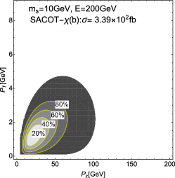
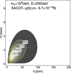
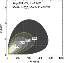
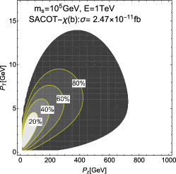
Figure 11: The $\tau$-momentum distribution in the CLFV DIS associated with bottom quark production in the SACOT-$\chi$ (thr) scheme. The threshold factor $S_{\rm thr}$ is included. The results for the scalar masses $m_{S}=10\,{\rm GeV}$ and $m_{S}=10^{5}\,{\rm GeV}$ are shown in the left and right columns, and the results for the initial electron beam energies $E_{e}=200\,{\rm GeV}$ and $E_{e}=1\,{\rm TeV}$ are shown in the two rows.

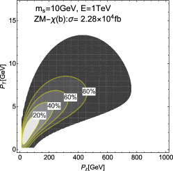
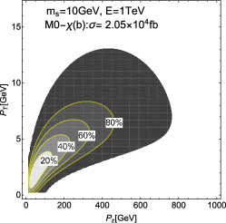
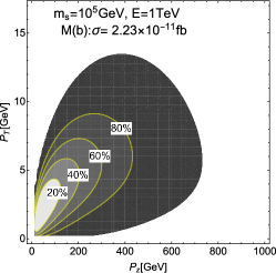
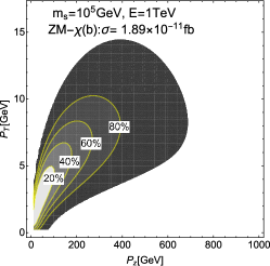
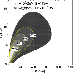
Figure 12: The $\tau$-momentum distribution for the components of SACOT-$\chi$ scheme for the bottom quark production at $E_{e}=1\,{\rm TeV}$. The results for the M, ZM-$\chi$, and M0-$\chi$ without the threshold factor are shown respectively in the first, second, and third columns. The scalar masses are $m_{S}=10\,{\rm GeV}$ and $m_{S}=10^{5}\,{\rm GeV}$ in the upper and lower rows.

In Fig. 11 we show the $\tau$-momentum distribution in the CLFV DIS associated with the bottom quark production in the SACOT-$\chi$(thr) scheme, where a combination of energies $E_{e}=200\,{\rm GeV},~{}1\,{\rm TeV}$ and the scalar masses $m_{S}=10\,{\rm GeV},~{}10^{5}\,{\rm GeV}$ is taken for each plot. One can see that the scalar mass does not affect much the shape of distribution for $E_{e}=200\,{\rm GeV}$, but the overall normalization. For $E_{e}=1\,{\rm TeV}$ there are sizable differences in the shape of the distribution between $m_{S}=10\,{\rm GeV}$ and $10^{5}\,{\rm GeV}$. Decomposing the cross section of SACOT-$\chi$(thr) scheme into the components one obtains the contributions:

$$\small\begin{split}\mbox{(i)}~{}~{}~{}~{}&\sigma_{b}^{{\rm SACOT\mathchar 45\relax\chi}}=\big{[}3.37+0.32(0.77)-0.30(0.75)\big{]}\times 10^{\,2}\,{\rm fb}~{}~{}~{}~{}=3.39(3.38)\times 10^{\,2}\,{\rm fb},\\ \mbox{(ii)}~{}~{}~{}&\sigma_{b}^{{\rm SACOT\mathchar 45\relax\chi}}=\big{[}4.93+1.53(2.28)-1.35(2.05)\big{]}\times 10^{\,4}\,{\rm fb}~{}~{}~{}~{}=5.11(5.15)\times 10^{\,4}\,{\rm fb},\\ \mbox{(iii)}~{}~{}&\sigma_{b}^{{\rm SACOT\mathchar 45\relax\chi}}=\big{[}6.61+1.02(2.24)-0.93(2.12)\big{]}\times 10^{-14}\,{\rm fb}~{}=6.70(6.73)\times 10^{-14}\,{\rm fb},\\ \mbox{(iv)}~{}~{}&\sigma_{b}^{{\rm SACOT\mathchar 45\relax\chi}}=\big{[}2.23+1.47(1.89)-1.22(1.60)\big{]}\times 10^{-11}\,{\rm fb}~{}=2.47(2.52)\times 10^{-11}\,{\rm fb},\end{split}$$ (39)

where the first/second/third number in the square parenthesis represents the M/ZM-$\chi$/M0-$\chi$ component with (without) the threshold factor $S_{\rm thr}$ for cases (i) $E_{e}=200\,{\rm GeV},~{}m_{S}=10\,{\rm GeV}$, (ii) $E_{e}=1\,{\rm TeV},~{}m_{S}=10\,{\rm GeV}$, (iii) $E_{e}=200\,{\rm GeV},~{}m_{S}=10^{5}\,{\rm GeV}$, and (iv) $E_{e}=1\,{\rm TeV},~{}m_{S}=10^{5}\,{\rm GeV}$. It is observed that the values of the ZM-$\chi$ and M0-$\chi$ components receive sizable threshold suppressions by the $S_{\rm thr}$, but the SACOT-$\chi$ cross section is approximately the same irrespective of inclusion of the threshold factor. It is because the contributions of the ZM-$\chi$(thr) and M0-$\chi$(thr) are the same size and cancel each other in the combination of $\big{[}F_{\phi,\rm thr}^{{\rm ZM\mathchar 45\relax\chi}}-F_{\phi,\rm thr}^{{\rm sub\mathchar 45\relax\chi}}\big{]}$ in the SACOT-$\chi$(thr) scheme.

In Fig. 12 we show the $\tau$-momentum distribution of the components for the bottom quark production at $E_{e}=1\,{\rm TeV}$, but without the threshold factor $S_{\rm thr}$. The upper and lower rows are the results for $m_{S}=10\,{\rm GeV}$ and $m_{S}=10^{5}\,{\rm GeV}$ respectively, and the first column is the result of M scheme, and the second and third columns are the results of the ZM-$\chi$ and M0-$\chi$ schemes respectively. It turns out that the largest contribution is coming from the massive scheme cross section. These observations lead that the massive scheme cross section is effective and nearly equal to the SACOT-$\chi$(thr) in the range of collision energy up to $E_{e}=1{\rm TeV}$ ($\sqrt{s}\simeq 45\,{\rm GeV}$). Effectiveness of massive scheme cross section in a wider range of collision energy will be discussed later (see Fig.18).

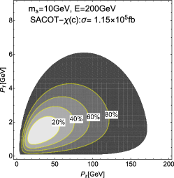
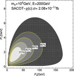
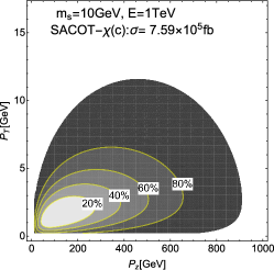
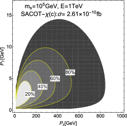
Figure 13: Same as Fig. 11, but for the charm quark productions: $m_{S}=10\,{\rm GeV}$ (left column) and $m_{S}=10^{5}\,{\rm GeV}$ (right column) for $E_{e}=200\,{\rm GeV}$ and $E_{e}=1\,{\rm TeV}$ in the two rows.

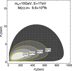
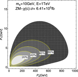
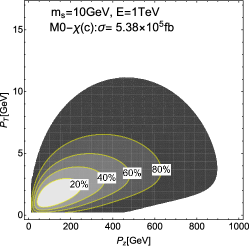
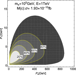
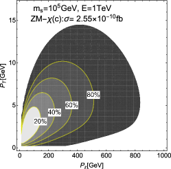
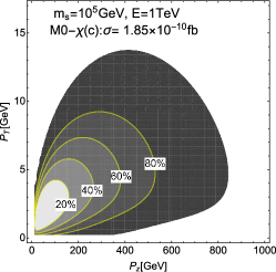
Figure 14: Same as Fig. 12, but for the charm quark productions. The results for the M, ZM-$\chi$, and M0-$\chi$ are shown in the three columns, and the results for $m_{S}=10\,{\rm GeV}$ and $m_{S}=10^{5}\,{\rm GeV}$ are shown in the two rows.

In Fig. 13 the $\tau$-momentum distribution in CLFV DIS associated with charm quark production is shown for $E_{e}=200\,{\rm GeV}$ and $E_{e}=1\,{\rm TeV}$. The distribution is more concentrated in the high-$p_{Z}$ region compared to one of the bottom quark production because the charm quark ($m_{c}=1.3\,{\rm GeV}$) is more relativistic than the bottom quark ($m_{b}=4.75\,{\rm GeV}$). The size of scalar mass affects the normalization and also the shape of the distribution. The cross sections in terms of components are given by:

$$\small\begin{split}\mbox{(i)}~{}~{}\sigma_{{\rm thr},c}^{{\rm SACOT\mathchar 45\relax\chi}}&=\big{[}9.30+8.64(9.98)-6.49(7.60)\big{]}\times 10^{\,4}\,{\rm fb}~{}~{}~{}~{}~{}=1.15(1.17)\times 10^{\,5}\,{\rm fb},\\ \mbox{(ii)}~{}~{}\sigma_{{\rm thr},c}^{{\rm SACOT\mathchar 45\relax\chi}}&=\big{[}6.60+5.85(6.41)-4.86(5.38)\big{]}\times 10^{\,5}\,{\rm fb}~{}~{}~{}~{}~{}=7.59(7.63)\times 10^{\,5}\,{\rm fb},\\ \mbox{(iii)}~{}~{}\sigma_{{\rm thr},c}^{{\rm SACOT\mathchar 45\relax\chi}}&=\big{[}1.56+1.78(1.99)-1.26(1.43)\big{]}\times 10^{-11}\,{\rm fb}~{}~{}=2.08(2.12)\times 10^{-11}\,{\rm fb},\\ \mbox{(iv)}~{}~{}\sigma_{{\rm thr},c}^{{\rm SACOT\mathchar 45\relax\chi}}&=\big{[}1.93+2.43(2.55)-1.75(1.85)\big{]}\times 10^{-10}\,{\rm fb}~{}~{}=2.61(2.62)\times 10^{-10}\,{\rm fb},\end{split}$$ (40)

where the first/second/third number in the square parenthesis represents the M/ZM-$\chi$/M0-$\chi$ contribution with (without) the threshold factor for (i) $E_{e}=200\,{\rm GeV},~{}m_{S}=10\,{\rm GeV}$, (ii) $E_{e}=1\,{\rm TeV},~{}m_{S}=10\,{\rm GeV}$, (iii) $E_{e}=200\,{\rm GeV},~{}m_{S}=10^{5}\,{\rm GeV}$, and (iv) $E_{e}=1\,{\rm TeV},~{}m_{S}=10^{5}\,{\rm GeV}$. In the components of SACOT-$\chi$(thr) cross section, the rates of M and ZM-$\chi$(thr) cross sections are the same size. For the charm quark production, dominance of only one component does not hold for $E_{e}=200\,{\rm GeV}$ and $E_{e}=1\,{\rm TeV}$.

It should be remembered that we have fixed the CLFV couplings by Eq. (38), which control the overall normalization of the cross section. Thus it is of great importance to find a sensitivity to the scalar mass in the shape of the distribution, which can be utilized for a detailed study to discriminate the structure of the CLFV interactions, namely for the separation of effects of coupling constants and of scalar mass.

IV.3 SACOT-$\chi$: $Q$-distribution

Here we rewrite the cross section as

$$\frac{d\sigma}{dQ} = \frac{1}{m_{\phi}^{4}}\,W_{\phi}(m_{\phi}^{2},Q^{2})\widetilde{M}_{\phi}(s,Q^{2}),$$ (41)

$$\widetilde{M}_{\phi}(s,Q^{2}) = \frac{(Q^{2})^{\frac{3}{2}}(Q^{2}+m_{\tau}^{2})}{8\pi s^{2}}M_{\phi}(s,Q^{2}),$$ (42)

$$W_{\phi}(m_{\phi}^{2},Q^{2}) = \left(\frac{m_{\phi}^{2}}{Q^{2}+m_{\phi}^{2}}\right)^{2},$$ (43)

where we have introduced a modified inverse moment $\widetilde{M}$ and a weighting factor $W_{\phi}$. The mediator mass can be set to $m_{\phi}=m_{S}$. Note that the product of $W_{\phi}$ and $\widetilde{M}_{\phi}$ gives $d\sigma/dQ$ not $d\sigma/dQ^{2}$ (up to $m_{\phi}^{4}$). The inverse moment $\widetilde{M}_{\phi}(s,Q^{2})$ is more adequate than the structure function to see which region of $Q$ contributes to the cross section.

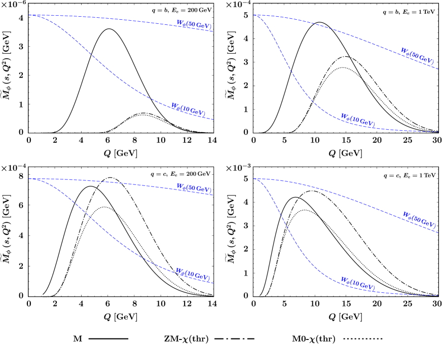
Figure 15: The inverse moment $\widetilde{M}_{\phi}(s,Q^{2})$ for each component of the SACOT-$\chi$(thr), and the weighting factor $W_{\phi}(m_{S}^{2},Q^{2})$ for $m_{S}=10\,{\rm GeV}$ and $m_{S}=50\,{\rm GeV}$. For visualization the weighting factor normalized to appropriate values are plotted. The results for bottom quark ($q=b$) and charm quark ($q=c$) are shown respectively in the upper and lower rows, and the beam energies are $E_{e}={\rm 200\,GeV}$ and $E_{e}={\rm 1\,TeV}$ in the left and right columns.

In Fig. 15, the inverse moments $\widetilde{M}_{\phi}(s,Q^{2})$ are plotted as functions of $Q$ for the bottom and charm quark productions in upper and lower rows, respectively. The results for $E_{e}=200\,{\rm GeV}$ and $E_{e}=1\,{\rm TeV}$ are shown in the left and right columns, respectively. In the plots one can see the following features of the inverse moment:

• The support of the M scheme inverse moment starts at low $Q$: the curve of the $\widetilde{M}_{\phi}$ in the M scheme rises from 0 at $Q\sim 2\,{\rm GeV}$ ($Q\sim 1\,{\rm GeV}$) for the bottom (charm) case. On the other hand, the curve of the $\widetilde{M}_{\phi}$ in the ZM-$\chi$(thr) scheme rises from 0 at $Q\sim 6\,{\rm GeV}$ ($Q\sim 2\,{\rm GeV}$) for the bottom (charm) case. Thus the cross section of the M scheme is superior in magnitude to that of the ZM-$\chi$(thr) in the very low-$Q^{2}$ region.

• The larger the beam energy $E_{e}$ the higher the maximum $Q$ for the support of the inverse moment in all the schemes. The relative size of ZM-$\chi$(thr) to that of the M scheme tends to grow with the beam energy.

These features due to the dynamics of the QCD (properties of the structure functions) together with the $Q$-dependence of the weighting function $W_{\phi}(m_{\phi}^{2},Q^{2})$ determine the relative importance of the M scheme contribution to that of ZM-$\chi$(thr) as a function of $m_{\phi}^{2}$ and $s$.

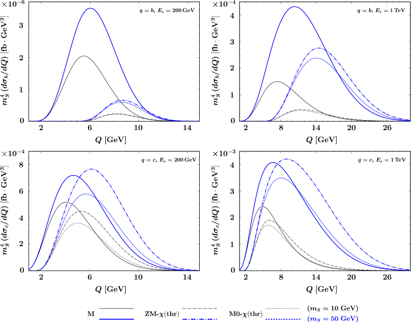
Figure 16: The CLFV DIS cross sections $m_{S}^{4}\,(d\sigma/dQ)$ are plotted as functions of $Q$. The results for bottom quark ($q=b$) and charm quark ($q=c$) are shown respectively in the upper and lower rows, and the beam energies are $E_{e}=200\,{\rm GeV}$ and $E_{e}=1\,{\rm TeV}$ in the left and right columns. The scalar masses are $m_{S}=10\,{\rm GeV}$(black lines) and $m_{S}=50\,{\rm GeV}$(blue lines).

In Fig. 16, the cross section $m_{S}^{4}\,d\sigma/dQ$ is plotted as a function of $Q$ for CLFV DIS associated with the heavy quark production. A prefactor $m_{S}^{4}$ is multiplied to scale out the leading $m_{S}$-dependence in the large-$m_{S}$ limit. The results for the bottom ($q=b$) and charm ($q=c$) quark productions are presented in the upper and lower rows, and the results for the beam energies of $E_{e}=200\,{\rm GeV}$ and $E_{e}=1\,{\rm TeV}$ are presented in the left and right columns. Two representative cases $m_{S}=10\,{\rm GeV}$ (black curves) and $m_{S}=50\,{\rm GeV}$ (blue curves) for the scalar mass are simulated. Note that $m_{S}=50\,{\rm GeV}$ is sufficiently large compared to typical momentum transfer $Q$ for $E_{e}=200\,{\rm GeV}$ and $E_{e}=1\,{\rm TeV}$ (see Figs. 15, 17), thus it corresponds approximately to a case of the large-$m_{S}$ limit. In the plots we observe the following:

• For the bottom quark production, the supports of the cross sections of M and ZM-$\chi$(thr) schemes start respectively at $Q\sim 2\,{\rm GeV}$ and $Q\sim 6\,{\rm GeV}$. The contribution from the region ${\cal R}_{Q}=\{Q|~{}2\,{\rm GeV}\leq Q\leq 6\,{\rm GeV}\}$ to the M scheme cross section is given by $\sigma^{{\rm M}}({\cal R}_{R})=\int_{{\cal R}_{Q}}(d\sigma^{{\rm M}}/dQ)dQ$ and it is large, while the contribution from the same region to ZM-$\chi$(thr) is $\sigma^{{\rm ZM\mathchar 45\relax\chi}}({\cal R}_{Q})=0$. This yields significantly large contribution exclusively to the M scheme cross section, leading the dominance of the M component in the SACOT-$\chi$(thr) cross section for $E_{e}=200\,{\rm GeV}$ and $E_{e}=1\,{\rm TeV}$. The difference $(\sigma_{\phi,{\rm thr}}^{{\rm ZM\mathchar 45\relax\chi}}-\sigma_{\phi,{\rm thr}}^{{\rm M0\mathchar 45\relax\chi}})$ is approximately 0 except the case of $m_{S}=50\,{\rm GeV}$ for $E_{e}=1\,{\rm TeV}$. The effect of the $Q^{2}$ evolution of the bottom PDF to the SACOT-$\chi$(thr) cross section is negligible for $m_{S}=10\,{\rm GeV}$ irrespective of the beam energy, and it is moderate for $m_{S}=10^{5}\,{\rm GeV}$ with $E_{e}=1\,{\rm TeV}$.

• For the charm quark production, all the components are approximately equal in magnitude, and the difference $(\sigma_{\phi,{\rm thr}}^{{\rm ZM\mathchar 45\relax\chi}}-\sigma_{\phi,{\rm thr}}^{{\rm M0\mathchar 45\relax\chi}})$ is large, thus $(\sigma_{\phi,{\rm thr}}^{{\rm SACOT\mathchar 45\relax\chi}}-\sigma_{\phi}^{{\rm M}})$ is also large. This means that the effect of $Q^{2}$ evolution for the charm PDF is large, therefore the deviation of M component from the SACOT-$\chi$(thr) becomes sizable. Breakdown of the M scheme dominance occurs depending on the value of scalar mass and also on beam energy $E_{e}$. Actually the cross section in ZM-$\chi$(thr) becomes dominant for large scalar mass $m_{S}=50\,{\rm GeV}$ (see also the case of $m_{S}=10^{5}\,{\rm GeV}$ in Eq. (40)).

• The M0-$\chi$(thr) curves are close to the ZM-$\chi$(thr) curves in the low-$Q^{2}$ region, while in the higher $Q$ they approach to the M scheme curves. This is expected by its construction; the subtraction term (=M0-$\chi$(thr)) should agree with M scheme contribution for $Q^{2}\gg m_{q}^{2}$ because the leading mass singularities are the same in both schemes, and the subtraction term should agree with ZM-$\chi$(thr) for $Q^{2}\sim m_{q}^{2}$ because the heavy quark PDFs are born in the region $\mu_{f}^{2}\sim m_{q}^{2}$ and $f_{q/N}(x,\mu_{f}^{2})$ are not evolved much. Indeed it is seen in all the plots that curves of M0-$\chi$(thr) interpolate the two schemes from low-$Q^{2}$ to high-$Q^{2}$ region between ZM-$\chi$ and M schemes.

There is one important difference between the CLFV DIS mediated by the massive scalar $\phi$ and standard neutral current DIS $eN\to eX$ where the massless photon is exchanged. The total cross section for the CLFV DIS contains the contribution from all the $Q$ region, and the relative importance of the low-$Q^{2}$ region versus large-$Q^{2}$ region is controlled not only by the collision energy $\sqrt{s}$ but also by the scalar mass $m_{S}$. Here the scalar mass $m_{S}$ plays a role of cut-off for the momentum transfer $Q$, and the contribution from the region of $Q\gtrsim m_{S}$ to the CLFV cross section is suppressed. This is contrasted with the normal DIS where the $Q$ region which contributes to the cross section is controlled solely by the collision energy $\sqrt{s}$.

IV.4 SACOT-$\chi$: Total cross section

Here we discuss the dependences of the total cross sections on the collision energy $\sqrt{s}$ and on the scalar mass $m_{S}$ in the SACOT-$\chi$(thr) scheme. In Fig. 17 the total cross sections $m_{S}^{4}\,\sigma_{q}$ for CLFV DIS associated with heavy quark productions are plotted as functions of scalar mass $m_{S}$. The results for bottom and charm quark productions are presented in the upper and lower rows, respectively, and the beam energies are $E_{e}=200\,{\rm GeV}$ and $E_{e}=1\,{\rm TeV}$ respectively in the left and right columns. The following behaviors concerning to the $m_{S}$-dependence can be read from the plots:

• For the bottom quark production, all the curves for SACOT-$\chi$(thr), M, ZM-$\chi$(thr), and sub-$\chi$(thr) converge to their asymptotic (constant) values in large-$m_{S}$ limit. The SACOT-$\chi$(thr) cross section fitted at the large-$m_{S}$ limit is $\sigma_{{\rm thr},b}^{{\rm SACOT\mathchar 45\relax\chi}}\approx(6.6+1.0-0.9)\cdot 10^{6}\,{\rm fb}\times(m_{S}/1\,{\rm GeV})^{-4}$, decomposing the components for M, ZM-$\chi$(thr), sub-$\chi$(thr), for $E_{e}=200\,{\rm GeV}$ and $\sigma_{{\rm thr},b}^{{\rm SACOT\mathchar 45\relax\chi}}\approx(2.2+1.5-1.2)\cdot 10^{9}\,{\rm fb}\times(m_{S}/1\,{\rm GeV})^{-4}$ for $E_{e}=1\,{\rm TeV}$, which agree with the values for $m_{S}=10^{5}\,{\rm GeV}$ in Eq. (39). The SACOT-$\chi$(thr) cross section evaluated at $m_{S}=50\,{\rm GeV}$ deviates from this asymptotic form by $4\%$ ($13\%$) for $E_{e}=200\,{\rm GeV}$ ($E_{e}=1\,{\rm TeV}$). This bears out that the value of $m_{S}=50\,{\rm GeV}$ can be regarded in a good approximation as the large-$m_{S}$ limit for beam energies $E_{e}\lesssim 1\,{\rm TeV}$. The plots for the bottom cross section also show that the M scheme cross section is a good approximation to the SACOT-$\chi$(thr), regardless of the value of $m_{S}$ for $E_{e}\lesssim 1\,{\rm TeV}$.

• For the charm quark production, all the curves for $E_{e}=200\,{\rm GeV}$ and $E_{e}=1\,{\rm TeV}$ converge to their asymptotic values similarly to the case of bottom quark production. The SACOT-$\chi$(thr) cross section fitted as the large-$m_{S}$ limit is $\sigma_{{\rm thr},c}^{{\rm SACOT\mathchar 45\relax\chi}}\approx(1.6+1.8-1.3)\cdot 10^{9}\,{\rm fb}\times(m_{S}/1\,{\rm GeV})^{-4}$ for $E_{e}=200\,{\rm GeV}$ and $\sigma_{{\rm thr},c}^{{\rm SACOT\mathchar 45\relax\chi}}\approx(1.9+2.4-1.8)\cdot 10^{10}\,{\rm fb}\times(m_{S}/1\,{\rm GeV})^{-4}$ for $E_{e}=1\,{\rm TeV}$, which agree with the values for $m_{S}=10^{5}\,{\rm GeV}$ in Eq. (40). Comparing the asymptotic large-$m_{S}$ limit with the values at $m_{S}=50\,{\rm GeV}$ bears out that $m_{S}=50\,{\rm GeV}$ can be regarded in a good approximation as the asymptotic large $m_{S}$-limit for beam energies $E_{e}\lesssim 1\,{\rm TeV}$. For the charm case, the ZM-$\chi$(thr) cross section is the dominant component for $m_{S}\gtrsim 15\,{\rm GeV}$ and $E_{e}\lesssim 1\,{\rm TeV}$, but there is still sizable corrections from the components M and sub-$\chi$(thr) to match with the value of the SACOT-$\chi$(thr) scheme cross section.

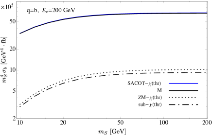
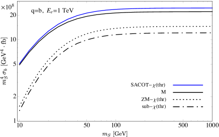
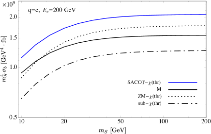
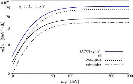
Figure 17: The total cross sections $m_{S}^{4}\,\sigma_{q}$ are plotted as functions of $m_{S}$. The results for bottom quark ($q=b$) and charm quark ($q=c$) are shown respectively in the upper and lower rows, and the beam energies are $E_{e}=200\,{\rm GeV}$ and $E_{e}=1\,{\rm TeV}$ in the left and right columns.

Figure 18: The components M, ZM-$\chi$, and M0-$\chi$ normalized to the SACOT-$\chi$ as functions of the collision energy $\sqrt{s}$: the ticks of upper horizontal axis indicate the corresponding beam energy $E_{e}$. The cross sections for the bottom and charm quark production are shown in the upper and lower rows. The scalar masses are $m_{S}=10\,{\rm GeV}$ and $m_{S}=10^{5}\,{\rm GeV}$ respectively in the left and right columns.

For comparison among the components of SACOT-$\chi$(thr) cross section in a wide range of the collision energy, the total cross sections are plotted in Fig. 18 as functions of $\sqrt{s}$ for bottom and charm quark productions. Numerical values for the cross sections in the SACOT-$\chi$(thr) scheme and its components are listed in Table 2. Concerning to the collision energy dependences following features can be observed from the plots:

• For the bottom quark production the dominance of the M scheme contribution holds for the small scalar mass $m_{S}=10\,{\rm GeV}$ in all the range of $\sqrt{s}$. But for the large scalar mass $m_{S}=10^{5}\,{\rm GeV}$ the ZM-$\chi$(thr) contribution becomes the dominant component for $\sqrt{s}\gtrsim 100\,{\rm GeV}$ ($E_{e}\gtrsim 5\,{\rm TeV}$). In large $\sqrt{s}$ limit for the case of $m_{S}=10^{5}\,{\rm GeV}$ the cross sections in M and ZM-$\chi$(thr) schemes coincide each other above $\sqrt{s}\approx 1\,{\rm TeV}$. Thus the M and sub-$\chi$(thr) terms cancels each other and the SACOT-$\chi$(thr) scheme cross section is approximated by the ZM-$\chi$(thr) cross section for $\sqrt{s}\gtrsim 1\,{\rm TeV}$, i.e. $\sigma_{{\rm thr},b}^{{\rm SACOT\mathchar 45\relax\chi}}\simeq\sigma_{{\rm thr},b}^{{\rm ZM\mathchar 45\relax\chi}}$ for $m_{S}=10^{5}\,{\rm GeV}$ and $\sqrt{s}\gtrsim 1\,{\rm TeV}$.

• For the charm quark production for small scalar mass $m_{S}=10\,{\rm GeV}$, there is no unique component which dominates the cross section in all the energy range, and all the components M, ZM-$\chi$(thr), and sub-$\chi$(thr) are equally important for the total cross section $\sigma_{{\rm thr},c}^{{\rm SACOT\mathchar 45\relax\chi}}$. On the other hand, for the large scalar mass $m_{S}=10^{5}\,{\rm GeV}$, the ZM-$\chi$ cross section describes the SACOT-$\chi$(thr) cross section well for all the energy range except $\sqrt{s}\lesssim 100\,{\rm GeV}$. Starting at $\sqrt{s}\sim 100\,{\rm GeV}$ the M and sub-$\chi$(thr) cross sections coincide so that they cancel each other in the SACOT-$\chi$(thr) cross section, i.e. $\sigma_{{\rm thr},c}^{{\rm SACOT\mathchar 45\relax\chi}}\simeq\sigma_{{\rm thr},c}^{{\rm ZM\mathchar 45\relax\chi}}$ for $m_{S}=10^{5}\,{\rm GeV}$.

Table 2: The total cross sections for CLFV DIS associated with bottom quark production in SACOT-$\chi$-thr and its components. For the ZM-$\chi$, M0-$\chi$ and SACOT-$\chi$ schemes, the threshold factor $S_{\rm thr}$ is taken into account.

$m_{S}~{}[\rm{GeV}]$	$E_{e}~{}{\rm[GeV]}$	$\sigma_{b}^{\rm M}~{}{\rm[fb]}$	$\sigma_{{\rm thr},b}^{{\rm ZM\mathchar 45\relax\chi}}~{}{\rm[fb]}$	$\sigma_{{\rm thr},b}^{{\rm M0\mathchar 45\relax\chi}}~{}{\rm[fb]}$	$\sigma_{{\rm thr},b}^{{\rm SACOT\mathchar 45\relax\chi}}~{}{\rm[fb]}$
	$10^{2}$	$2.08\times 10^{-1}$	$1.95\times 10^{-3}$	$2.32\times 10^{-3}$	$2.07\times 10^{-1}$
	$10^{3}$	$4.93\times 10^{4}$	$1.53\times 10^{4}$	$1.35\times 10^{4}$	$5.11\times 10^{4}$
$10$	$10^{4}$	$7.32\times 10^{5}$	$2.87\times 10^{5}$	$2.66\times 10^{5}$	$7.53\times 10^{5}$
	$10^{5}$	$3.72\times 10^{6}$	$1.54\times 10^{6}$	$1.51\times 10^{6}$	$3.75\times 10^{6}$
	$10^{6}$	$1.18\times 10^{7}$	$4.90\times 10^{6}$	$5.18\times 10^{6}$	$1.15\times 10^{7}$
	$10^{7}$	$2.99\times 10^{7}$	$1.22\times 10^{7}$	$1.39\times 10^{7}$	$2.81\times 10^{7}$
	$10^{2}$	$3.17\times 10^{-17}$	$4.06\times 10^{-19}$	$4.74\times 10^{-19}$	$3.17\times 10^{-17}$
	$10^{3}$	$2.23\times 10^{-11}$	$1.47\times 10^{-11}$	$1.22\times 10^{-11}$	$2.47\times 10^{-11}$
$10^{5}$	$10^{4}$	$1.27\times 10^{-9}$	$1.32\times 10^{-9}$	$1.07\times 10^{-9}$	$1.51\times 10^{-9}$
	$10^{5}$	$2.57\times 10^{-8}$	$3.03\times 10^{-8}$	$2.44\times 10^{-8}$	$3.16\times 10^{-8}$
	$10^{6}$	$3.66\times 10^{-7}$	$4.54\times 10^{-7}$	$3.61\times 10^{-7}$	$4.59\times 10^{-7}$
	$10^{7}$	$4.50\times 10^{-6}$	$5.72\times 10^{-6}$	$4.49\times 10^{-6}$	$5.73\times 10^{-6}$
$m_{S}~{}[\rm{GeV}]$	$E_{e}~{}{\rm[GeV]}$	$\sigma_{c}^{\rm M}~{}{\rm[fb]}$	$\sigma_{{\rm thr},c}^{{\rm ZM\mathchar 45\relax\chi}}~{}{\rm[fb]}$	$\sigma_{{\rm thr},c}^{{\rm M0\mathchar 45\relax\chi}}~{}{\rm[fb]}$	$\sigma_{{\rm thr},c}^{{\rm SACOT\mathchar 45\relax\chi}}~{}{\rm[fb]}$
	$10^{2}$	$2.74\times 10^{4}$	$2.45\times 10^{4}$	$1.79\times 10^{4}$	$3.40\times 10^{4}$
	$10^{3}$	$6.59\times 10^{5}$	$5.85\times 10^{5}$	$4.86\times 10^{5}$	$7.58\times 10^{5}$
$10$	$10^{4}$	$4.15\times 10^{6}$	$3.25\times 10^{6}$	$3.13\times 10^{6}$	$4.27\times 10^{6}$
	$10^{5}$	$1.46\times 10^{7}$	$9.73\times 10^{6}$	$1.11\times 10^{7}$	$1.32\times 10^{7}$
	$10^{6}$	$3.83\times 10^{7}$	$2.15\times 10^{7}$	$2.96\times 10^{7}$	$3.02\times 10^{7}$
	$10^{7}$	$8.68\times 10^{7}$	$4.19\times 10^{7}$	$6.78\times 10^{7}$	$6.09\times 10^{7}$
	$10^{2}$	$3.86\times 10^{-12}$	$3.99\times 10^{-12}$	$2.83\times 10^{-12}$	$5.03\times 10^{-12}$
	$10^{3}$	$1.93\times 10^{-10}$	$2.43\times 10^{-10}$	$1.75\times 10^{-10}$	$2.61\times 10^{-10}$
$10^{5}$	$10^{4}$	$3.51\times 10^{-9}$	$4.64\times 10^{-9}$	$3.41\times 10^{-9}$	$4.75\times 10^{-9}$
	$10^{5}$	$4.66\times 10^{-8}$	$6.29\times 10^{-8}$	$4.62\times 10^{-8}$	$6.33\times 10^{-8}$
	$10^{6}$	$5.48\times 10^{-7}$	$7.50\times 10^{-7}$	$5.47\times 10^{-7}$	$7.50\times 10^{-7}$
	$10^{7}$	$6.09\times 10^{-6}$	$8.45\times 10^{-6}$	$6.09\times 10^{-6}$	$8.44\times 10^{-6}$

V Summary

In this article, we have considered a scenario where a CLFV (pseudo-)scalar mediator couples dominantly to heavy quarks and studied the CLFV DIS associated with heavy quark productions $\ell_{i}N\to\ell_{j}q\bar{q}X$ ($q=b,c$). The CLFV DIS cross sections are written in terms of the leptonic and the hadronic parts. We have computed the heavy quark contributions to the structure function in the SACOT-$\chi$(thr), M, ZM-$\chi$(thr), and M0-$\chi$(thr) schemes and presented their results. We have examined three improvements for the threshold behavior of the structure function: the $\chi$-rescaling, choice of factorization scale $\mu_{f}$, and inclusion of the threshold factor $S_{\rm thr}$. To our best knowledge the present article is the first application of the SACOT-$\chi$(thr) scheme for the CLFV DIS associated with heavy quark productions. We have shown that only the SACOT-$\chi$(thr) scheme provides a reliable theory prediction for the CLFV DIS cross section in the wide kinematical region and in the full parameter space. Thus the systematic study for the CLFV signal search including the full DIS kinematical information will be available in the SACOT-$\chi$(thr) scheme.

For the structure function we have made a comparison among the different computational schemes and observed that the $\chi$-rescaling is effective in $Q\lesssim 100\,(50)$ GeV for the bottom (charm) quark production. It is mandatory to incorporate the $\chi$-rescaling to predict the structure function especially on the threshold behavior of the heavy quark productions.

We also made a detailed analysis on the collision energy dependence and the mediator mass dependence of the heavy quark production cross sections focusing on the beam energies up to $E_{e}=1\,{\rm TeV}$. For the bottom quark production, we showed that the M scheme cross section approximates that of the SACOT-$\chi$(thr) irrespective of the size of the scalar mass. For the charm quark production, we showed that the ZM-$\chi$(thr) cross section approximates that of the SACOT-$\chi$(thr) for $m_{S}\gtrsim 50\,{\rm GeV}$, but for the small scalar mass $\sim 10\,{\rm GeV}$ the M scheme cross section becomes the dominant component for SACOT-$\chi$(thr). We found that the ratio of the contributions in the massive and the zero-mass schemes strongly depends on the mediator mass. This is because when the mediator mass is small, the contributions from the low-$Q^{2}$ region are enhanced, for which the M scheme contribution is superior. We conclude that the SACOT-$\chi$(thr) prescription is indispensable to obtain the reliable sensitivity to the CLFV interactions in the next generation experiments of the energy range $E_{e}\lesssim 1\,{\rm TeV}$.

To utilize the processes for the CLFV signal searches, we propose the measurements of the total cross sections and the momentum distributions $d^{2}\sigma/d\bm{p}$ of the final lepton. The normalizations of the total cross sections depend on the combination of CLFV mediator couplings $|\rho_{qq}^{\phi}|^{2}(|\rho_{ij}^{\phi}|^{2}+|\rho_{ji}^{\phi}|^{2})$ and $m_{S}$, while the (normalized) momentum distributions depend on $m_{S}$. We have shown for the case of $eN\to\tau q\bar{q}X$ that the momentum distributions can have a sensitivity on the size of scalar mass. To make a definite conclusion on the feasibility of the simultaneous determination of the CLFV couplings and the scalar mass, more efforts have to be devoted to improve the precision of the theory computations. The issues of the scale dependence, PDF uncertainties, QCD radiative corrections, etc., have to be addressed together with more detailed simulation study taking the experimental uncertainties into account, which are beyond the scope of the present article, but we render them for a future work.

For the present model Lagrangian, it is known that the other types of subprocesses also contribute to the CLFV DIS via the gluonic operator ($\sim\phi\,G^{a}_{\mu\nu}G^{a\,\mu\nu}$) and the photonic dipole operator ($\sim\bar{\ell}_{i}\sigma_{\mu\nu}\ell_{j}F^{\mu\nu}$) which generate the processes $\ell_{i}g\to\ell_{j}g$ and $\ell_{i}q_{l}\to\ell_{j}q_{l}$ ($q_{l}$ being the light quarks). The comprehensive analysis of the DIS observables taking these subprocesses into account is required to disentangle the type of the CLFV operators and eventually to unravel the properties of CLFV mediators. We leave these issues for our future works.

Appendix A Physical region of DIS kinematics

A.1 Range of $(x,y)$ in generic case

We derive the physical region of kinematical variable $x$ and $y$ for CLFV DIS process $\ell_{i}(k_{i})p(k_{p})\to\ell_{j}(k_{j})\hat{X}(k_{X})$, where $\hat{X}$ can be one particle or a multi-particle system. We assume that the initial QCD parton $p$ is massless with momentum $k_{p}=\xi P$, and other particles are massive: $k_{i}^{2}=m_{i}^{2},k_{p}^{2}=0,k_{j}^{2}=m_{j}^{2}$, and $k_{X}^{2}=w^{2}$. Similar analyses can be found in literatures Albright and Jarlskog (1975); Hagiwara et al. (2003).

First we express the kinematical variables in the center-of-mass frame of lepton and parton, where lepton energies are given by

$$E_{i}~{}=~{}\frac{\hat{s}+m_{i}^{2}}{2\sqrt{\hat{s}}},\hskip 11.38109ptE_{j}~{}=~{}\frac{\hat{s}+m_{j}^{2}-w^{2}}{2\sqrt{\hat{s}}},$$ (44)

where $\hat{s}=(k_{p}+k_{i})^{2}$ is related to the lepton-nucleon collision energy squared $s=(P+k_{i})^{2}$ by $\hat{s}-m_{i}^{2}=\xi\,(s-m_{i}^{2})$. The momentum transfer $Q^{2}=-q^{2}=-(k_{i}-k_{j})^{2}$ is given by $Q^{2}=-(m_{i}^{2}+m_{j}^{2})+2E_{i}E_{j}-2|\bm{k}_{i}||\bm{k}_{j}|\cos\theta_{ij}$ in the center-of-mass frame, where the product of spacial momenta in the last term can be replaced by $|\bm{k}_{i}||\bm{k}_{j}|=\sqrt{E_{i}^{2}-m_{i}^{2}}\sqrt{E_{j}^{2}-m_{j}^{2}}$. Now the angle $\theta_{ij}$ can be written as

$$\begin{split}\cos\theta_{ij}=\frac{2E_{i}E_{j}-xy(s-m_{i}^{2})-(m_{i}^{2}+m_{j}^{2})}{2\sqrt{E_{i}^{2}-m_{i}^{2}}\sqrt{E_{j}^{2}-m_{j}^{2}}},\end{split}$$ (45)

where $Q^{2}=xy(s-m_{i}^{2})$ is used. The constraint $|\cos\theta_{ij}|\leq 1$ leads to an inequality

$$\begin{split}\bigl{[}2E_{i}E_{j}-xy\left(s-m_{i}^{2}\right)-\left(m_{i}^{2}+m_{j}^{2}\right)\bigr{]}^{2}\leq 4(E_{i}^{2}-m_{i}^{2})(E_{j}^{2}-m_{j}^{2}).\end{split}$$ (46)

Substituting the lepton energies by Eq. (44), we obtain

$$y\,\big{\{}(1-y)\big{[}x(s-m_{i}^{2})+m_{i}^{2}\big{]}-m_{j}^{2}\big{\}}\geq 0,$$ (47)

where we used $w^{2}=(k_{p}+q)^{2}=y(\hat{s}-m_{i}^{2})(1-x/\xi)$. This condition determines the upper bound of the inelasticity $y$

$$\begin{split}y\leq 1-\frac{r_{j}}{x+r_{i}}.\end{split}$$ (48)

Here we introduced dimensionless masses $r_{a}~{}(a=i,j)$

$$r_{i} = \frac{m_{i}^{2}}{s-m_{i}^{2}},\hskip 14.22636ptr_{j}~{}=~{}\frac{m_{j}^{2}}{s-m_{i}^{2}}.$$ (49)

The lower one is bound by the partonic phase space. We express the inelasticity parameter $y$ in terms of $x$ and $w^{2}$

$$y = \frac{1}{\xi-x}\left(\frac{w^{2}}{s-m_{i}^{2}}\right).$$ (50)

The momentum fraction $\xi$ is expressed in terms of Lorentz invariance as $\xi=x\,\left(Q^{2}+\omega^{2}\right)/Q^{2}$, and its minimum needs to be less than $x$;

$$\begin{split}\xi=x\left(\frac{Q^{2}+w_{\text{min}}^{2}}{Q^{2}}\right)\geq x.\end{split}$$ (51)

Thus the lower bound of $y$ is given by the production threshold of $w^{2}_{\rm min}$ with maximum momentum fraction $\xi=1$:

$$y\geq\frac{1}{1-x}\left(\frac{w^{2}_{\rm min}}{s-m_{i}^{2}}\right)$$ (52)

Thus the physical range of $y$ for fixed $x$ is given by $y_{\rm min}\leq y\leq y_{\rm max}$ with

$$y_{\rm min}(x)~{}=~{}\frac{r_{\rm min}}{1-x},\hskip 28.45274pty_{\rm max}(x)~{}=~{}1-\frac{r_{j}}{x+r_{i}},$$ (53)

where $r_{\rm min}\equiv w_{\rm min}^{2}/(s-m_{i}^{2})$.

The physical range of $x$ can be obtained by requiring that the lower bound on $y$ should be smaller than the upper one, namely $y_{\rm min}(x)\leq y_{\rm max}(x)$ should hold. This yields a relation

$$\begin{split}x^{2}-(1-r_{i}+r_{j}-r_{\rm min})x-(r_{i}-r_{j}-r_{i}\,r_{\rm min})\leq 0.\end{split}$$ (54)

Solving the quadratic inequality for $x$, we find the range $x_{-}\leq x\leq x_{+}$ with

$$x_{\pm} = \frac{1}{2}\bigg{[}\left(1-r_{i}+r_{j}-r_{\rm min}\right)\pm\sqrt{(1-r_{i}+r_{j}-r_{\rm min})^{2}+4(r_{i}-r_{j}-r_{i}r_{\rm min})}\bigg{]}.$$ (55)

A.2 Heavy quark pair production in terms of $(x,y)$

Here we give concrete expression for the physical region by taking electron and tau leptons as initial and final leptons, and a heavy quark pair of mass $m_{q}$ in the hadronic part, i.e. $\hat{X}=q\bar{q}$. We ignore the electron mass, but tau and heavy quark masses are kept. In this case Eq. (53) reduces to

$$y_{\rm min}(x) = \frac{4m_{q}^{2}}{(1-x)s},\hskip 28.45274pty_{\rm max}(x)~{}=~{}1-\frac{m_{\tau}^{2}}{xs},$$ (56)

and Eq. (55) reduces to

$$x_{\pm} = \frac{1}{2}\bigg{[}1+\frac{m_{\tau}^{2}}{s}-\frac{4m_{q}^{2}}{s}\pm\sqrt{\left(1+\frac{m_{\tau}^{2}}{s}-\frac{4m_{q}^{2}}{s}\right)^{2}-4\frac{m_{\tau}^{2}}{s}}~{}\bigg{]},$$ (57)

where the minimum of $w^{2}$ has been substituted by $4m_{q}^{2}$.

A.3 Heavy quark pair production in terms of $(x,Q^{2})$

When one takes $(x,Q^{2})$ as independent variables instead of $(x,y)$, the relation $xy=Q^{2}/s$ can be used. The physical region for $x$ is given by $x_{\rm min}(s,Q^{2})\leq x\leq x_{\rm max}(Q^{2})$ with

$$x_{\rm min}(s,Q^{2})~{}=~{}\frac{Q^{2}+m_{\tau}^{2}}{s},\hskip 28.45274ptx_{\rm max}(Q^{2})~{}=~{}\frac{Q^{2}}{Q^{2}+4m_{q}^{2}},$$ (58)

and for $Q^{2}$ the physical region is $Q_{-}^{2}\leq Q^{2}\leq Q_{+}^{2}$ with

$$Q^{2}_{\pm} = sx_{\pm}-m_{\tau}^{2},$$ (59)

where $x_{\pm}$ is defined in Eq. (57).

References

- Kuno and Okada (2001) Y. Kuno and Y. Okada, Rev. Mod. Phys. 73, 151 (2001), eprint hep-ph/9909265.
- Raidal et al. (2008) M. Raidal et al., Eur. Phys. J. C57, 13 (2008), eprint 0801.1826.
- Huber (2003) S. J. Huber, Nucl. Phys. B666, 269 (2003), eprint hep-ph/0303183.
- Moreau and Silva-Marcos (2006) G. Moreau and J. Silva-Marcos, JHEP 03, 090 (2006), eprint hep-ph/0602155.
- Agashe et al. (2006) K. Agashe, A. E. Blechman, and F. Petriello, Phys. Rev. D 74, 053011 (2006), eprint hep-ph/0606021.
- Davidson et al. (2008) S. Davidson, G. Isidori, and S. Uhlig, Phys. Lett. B663, 73 (2008), eprint 0711.3376.
- Kanemura et al. (2006) S. Kanemura, T. Ota, and K. Tsumura, Phys. Rev. D 73, 016006 (2006), eprint hep-ph/0505191.
- Davidson and Grenier (2010) S. Davidson and G. J. Grenier, Phys. Rev. D 81, 095016 (2010), eprint 1001.0434.
- Crivellin et al. (2013) A. Crivellin, A. Kokulu, and C. Greub, Phys. Rev. D 87, 094031 (2013), eprint 1303.5877.
- Botella et al. (2016) F. Botella, G. Branco, M. Nebot, and M. Rebelo, Eur. Phys. J. C 76, 161 (2016), eprint 1508.05101.
- Crivellin et al. (2021) A. Crivellin, C. Greub, D. Müller, and F. Saturnino, JHEP 02, 182 (2021), eprint 2010.06593.
- Tsumura and Velasco-Sevilla (2010) K. Tsumura and L. Velasco-Sevilla, Phys. Rev. D 81, 036012 (2010), eprint 0911.2149.
- Agashe et al. (2005) K. Agashe, M. Papucci, G. Perez, and D. Pirjol (2005), eprint hep-ph/0509117.
- Gninenko et al. (2002) S. N. Gninenko, M. M. Kirsanov, N. V. Krasnikov, and V. A. Matveev, Mod. Phys. Lett. A17, 1407 (2002), eprint hep-ph/0106302.
- Sher and Turan (2004) M. Sher and I. Turan, Phys. Rev. D69, 017302 (2004), eprint hep-ph/0309183.
- Kanemura et al. (2005) S. Kanemura, Y. Kuno, M. Kuze, and T. Ota, Phys. Lett. B607, 165 (2005), eprint hep-ph/0410044.
- Gonderinger and Ramsey-Musolf (2010) M. Gonderinger and M. J. Ramsey-Musolf, JHEP 11, 045 (2010), [Erratum: JHEP 05, 047 (2012)], eprint 1006.5063.
- Bolanos et al. (2013) A. Bolanos, A. Fernandez, A. Moyotl, and G. Tavares-Velasco, Phys. Rev. D 87, 016004 (2013), eprint 1212.0904.
- Liao and Wu (2016) W. Liao and X.-H. Wu, Phys. Rev. D 93, 016011 (2016), eprint 1512.01951.
- Abada et al. (2017) A. Abada, V. De Romeri, J. Orloff, and A. Teixeira, Eur. Phys. J. C 77, 304 (2017), eprint 1612.05548.
- Takeuchi et al. (2017) M. Takeuchi, Y. Uesaka, and M. Yamanaka, Phys. Lett. B772, 279 (2017), eprint 1705.01059.
- Gninenko et al. (2018) S. Gninenko, S. Kovalenko, S. Kuleshov, V. E. Lyubovitskij, and A. S. Zhevlakov, Phys. Rev. D 98, 015007 (2018), eprint 1804.05550.
- Antusch et al. (2020) S. Antusch, A. Hammad, and A. Rashed, Phys. Lett. B 810, 135796 (2020), eprint 2003.11091.
- Husek et al. (2021) T. Husek, K. Monsalvez-Pozo, and J. Portoles, JHEP 01, 059 (2021), eprint 2009.10428.
- Cirigliano et al. (2021) V. Cirigliano, K. Fuyuto, C. Lee, E. Mereghetti, and B. Yan, JHEP 03, 256 (2021), eprint 2102.06176.
- Antusch et al. (2021) S. Antusch, A. Hammad, and A. Rashed, JHEP 03, 230 (2021), eprint 2010.08907.
- Cakir et al. (2009) O. Cakir, A. Senol, and A. Tasci, EPL 88, 11002 (2009), eprint 0905.4347.
- Han and Mellado (2010) T. Han and B. Mellado, Phys. Rev. D82, 016009 (2010), eprint 0909.2460.
- Liang et al. (2010) H. Liang, X.-G. He, W.-G. Ma, S.-M. Wang, and R.-Y. Zhang, JHEP 09, 023 (2010), eprint 1006.5534.
- Blaksley et al. (2011) C. Blaksley, M. Blennow, F. Bonnet, P. Coloma, and E. Fernandez-Martinez, Nucl. Phys. B 852, 353 (2011), eprint 1105.0308.
- Biswal et al. (2012) S. S. Biswal, R. M. Godbole, B. Mellado, and S. Raychaudhuri, Phys. Rev. Lett. 109, 261801 (2012), eprint 1203.6285.
- Dutta et al. (2015) S. Dutta, A. Goyal, M. Kumar, and B. Mellado, Eur. Phys. J. C75, 577 (2015), eprint 1307.1688.
- Li et al. (2018) R. Li, X.-M. Shen, K. Wang, T. Xu, L. Zhang, and G. Zhu, Phys. Rev. D97, 075043 (2018), eprint 1711.05607.
- Curtin et al. (2018) D. Curtin, K. Deshpande, O. Fischer, and J. Zurita, JHEP 07, 024 (2018), eprint 1712.07135.
- Li et al. (2019) S.-Y. Li, Z.-G. Si, and X.-H. Yang, Phys. Lett. B 795, 49 (2019), eprint 1811.10313.
- Azuelos et al. (2020) G. Azuelos, M. D’Onofrio, S. Iwamoto, and K. Wang, Phys. Rev. D 101, 095015 (2020), eprint 1912.03823.
- Aktas et al. (2007) A. Aktas et al. (H1), Eur. Phys. J. C 52, 833 (2007), eprint hep-ex/0703004.
- Aaron et al. (2011) F. Aaron et al. (H1), Phys. Lett. B 701, 20 (2011), eprint 1103.4938.
- Accardi et al. (2016) A. Accardi et al., Eur. Phys. J. A 52, 268 (2016), eprint 1212.1701.
- Abelleira Fernandez et al. (2012) J. L. Abelleira Fernandez et al. (LHeC Study Group), J. Phys. G39, 075001 (2012), eprint 1206.2913.
- Aivazis et al. (1994a) M. A. G. Aivazis, F. I. Olness, and W.-K. Tung, Phys. Rev. D 50, 3085 (1994a), eprint hep-ph/9312318.
- Aivazis et al. (1994b) M. A. G. Aivazis, J. C. Collins, F. I. Olness, and W.-K. Tung, Phys. Rev. D50, 3102 (1994b), eprint hep-ph/9312319.
- Buza et al. (1998) M. Buza, Y. Matiounine, J. Smith, and W. L. van Neerven, Eur. Phys. J. C 1, 301 (1998), eprint hep-ph/9612398.
- Cacciari et al. (1998) M. Cacciari, M. Greco, and P. Nason, JHEP 05, 007 (1998), eprint hep-ph/9803400.
- Collins (1998) J. C. Collins, Phys. Rev. D 58, 094002 (1998), eprint hep-ph/9806259.
- Forte et al. (2010) S. Forte, E. Laenen, P. Nason, and J. Rojo, Nucl. Phys. B 834, 116 (2010), eprint 1001.2312.
- Krämer et al. (2000) M. Krämer, F. I. Olness, and D. E. Soper, Phys. Rev. D 62, 096007 (2000), eprint hep-ph/0003035.
- Tung et al. (2002) W.-K. Tung, S. Kretzer, and C. Schmidt, J. Phys. G 28, 983 (2002), eprint hep-ph/0110247.
- Kretzer et al. (2004) S. Kretzer, H. L. Lai, F. I. Olness, and W. K. Tung, Phys. Rev. D 69, 114005 (2004), eprint hep-ph/0307022.
- Stavreva et al. (2012) T. Stavreva, F. I. Olness, I. Schienbein, T. Jezo, A. Kusina, K. Kovarik, and J. Y. Yu, Phys. Rev. D 85, 114014 (2012), eprint 1203.0282.
- Gribov and Lipatov (1972) V. N. Gribov and L. N. Lipatov, Sov. J. Nucl. Phys. 15, 438 (1972).
- Altarelli and Parisi (1977) G. Altarelli and G. Parisi, Nucl. Phys. B 126, 298 (1977).
- Barnett (1976) R. M. Barnett, Phys. Rev. Lett. 36, 1163 (1976).
- Dulat et al. (2016) S. Dulat, T.-J. Hou, J. Gao, M. Guzzi, J. Huston, P. Nadolsky, J. Pumplin, C. Schmidt, D. Stump, and C. P. Yuan, Phys. Rev. D 93, 033006 (2016), eprint 1506.07443.
- Albright and Jarlskog (1975) C. H. Albright and C. Jarlskog, Nucl. Phys. B84, 467 (1975).
- Hagiwara et al. (2003) K. Hagiwara, K. Mawatari, and H. Yokoya, Nucl. Phys. B668, 364 (2003), [Erratum: Nucl. Phys.B701,405(2004)], eprint hep-ph/0305324.