High-frequency expansions for time-periodic Lindblad generators

Abstract

Floquet engineering of isolated systems is often based on the concept of the effective time-independent Floquet Hamiltonian, which describes the stroboscopic evolution of a periodically driven quantum system in steps of the driving period and which is routinely obtained analytically using high-frequency expansions. The generalization of these concepts to open quantum systems described by a Markovian master equation of Lindblad type turns out to be non-trivial: On the one hand, already for a two-level system two different phases can be distinguished, where the effective time-independent Floquet generator (describing the stroboscopic evolution) is either again Markovian and of Lindblad type or not. On the other hand, even though in the high-frequency regime a Lindbladian Floquet generator (Floquet Lindbladian) is numerically found to exist, this behaviour is, curiously, not correctly reproduced within analytical high-frequency expansions. Here, we demonstrate that a proper Floquet Lindbladian can still be obtained from a high-frequency expansion, when treating the problem in a suitably chosen rotating frame. Within this approach, we can then also describe the transition to a phase at lower driving frequencies, where no Floquet Lindbladian exists, and show that the emerging non-Markovianity of the Floquet generator can entirely be attributed to the micromotion of the open driven system.

I Introduction

Floquet engineering, that is the idea of manipulating the properties of a coherent quantum system by means of strong time-periodic driving, has been successfully applied to artificial many-body systems of ultracold atoms in optical lattices Aidelsburger et al. (2011); Struck et al. (2013); Gregor Jotzu AND Michael Messer AND Rémi Desbuquois et al. (2014); Aidelsburger et al. (2015); Fläschner et al. (2016); Eckardt (2017); Tarnowski et al. (2019); Viebahn et al. (2021). These systems are well isolated from their environment and therefore well described by the Schrödinger equation. However, with the recent progress in the engineering of quantum materials as well as complex photonic many-body systems Houck et al. (2012); Georgescu et al. (2014), also the control of these systems via periodic forcing becomes an interesting and promising perspective. They are typically interacting with an environment, which introduces dissipation to the system’s dynamics; see, e.g., Ref. Houck et al. (2012). It is, therefore, desirable to extend the concept of Floquet engineering to open quantum systems. In this context, two questions are of interest. The first one concerns the properties of the non-equilibrium steady state that such open periodically modulated systems approach in the long-time limit Breuer et al. (2000); Ketzmerick and Wustmann (2010); Vorberg et al. (2013); Shirai et al. (2015); Seetharam et al. (2015); Dehghani et al. (2015); Iadecola et al. (2015); Vorberg et al. (2015); Shirai et al. (2016); Letscher et al. (2017); Schnell et al. (2018); Chong et al. (2018); Qin et al. (2018). The second question, which will be discussed in this paper, concerns the transient dynamics of these systems. Here, analogously to the Floquet engineering of isolated quantum systems, one can ask, whether it is possible to find an effective time-independent description of the stroboscopic dynamics of the system Schnell et al. (2020); Haddadfarshi et al. (2015); Reimer et al. (2018); Restrepo et al. (2016); Dai et al. (2016, 2017); Hotz and Schaller (2021); Szczygielski (2021); Gunderson et al. (2021); Mizuta et al. (2021).

While for a closed system the stroboscopic dynamics can always be recast into an effective coherent evolution governed by a time-independent Floquet Hamiltonian Eckardt and Anisimovas (2015); Eckardt (2017), it is not obvious whether such a mapping exists for an open periodically modulated system. More specifically, when considering the Markovian evolution described by Lindblad-type master equations, the question is whether the stroboscopic dynamics can be described by an effective time-independent Floquet generator of the Lindblad type (henceforth addressed as Floquet Lindbladian). The existence of such Floquet Lindbladians has implicitly been assumed in recent works Haddadfarshi et al. (2015); Restrepo et al. (2016); Dai et al. (2016, 2017). However, in Ref. Schnell et al. (2020) it was shown that, already for a simple two-level system, there is no guarantee that such an operator exists. Namely, extensive parameter regions were found, where it does not exist, while in other extensive parameter regions, including the high-frequency limit, it does exist.

The high-frequency regime plays an important role for Floquet engineering of isolated systems. On the one hand, it is appealing because in this regime unwanted heating via resonant excitations is suppressed Eckardt (2017); Eckardt and Anisimovas (2015); Weinberg et al. (2015); Bilitewski and Cooper (2015); Wintersperger et al. (2020). On the other hand, it is possible to calculate the Floquet Hamiltonian by using systematic high-frequency expansions, such as the Magnus expansion Blanes et al. (2009), and thus to analytically predict the properties of the Floquet system. It is, therefore, very natural to generalise such high-frequency expansions to open systems, as it has been done in various recent papers Haddadfarshi et al. (2015); Restrepo et al. (2016); Dai et al. (2016, 2017); Mizuta et al. (2021); Ikeda et al. (2021). However, it was observed that the corresponding expansions usually do not provide time-independent Floquet generators of Lindblad type Haddadfarshi et al. (2015); Reimer et al. (2018); Mizuta et al. (2021). Below we will demonstrate this failure of the Magnus expansion for the model used in Ref. Schnell et al. (2020), despite the fact that the Floquet Lindbladian was explicitly shown to exist.

In this paper, we address the question, whether it is possible to construct a high-frequency expansion that is consistent with respect to the expected Lindblad-type stroboscopic evolution of the model. For this purpose, we compare four different approaches. Firstly, they are distinguished by the expansion technique they are based on, (i) a Magnus expansion Blanes et al. (2009) or (ii) a van-Vleck-type high-frequency expansion Eckardt and Anisimovas (2015). Secondly, they differ by the reference frame, in which the model system is treated, i.e., either (a) in the direct frame or (b) in a suitably chosen rotating frame. We find that it is the appropriately chosen rotating reference frame [approach (b)], which allows to compute Lindblad-type Floquet generators in the high-frequency limit for our model. As a second major result, we find that the break-down of the existence of a Floquet Lindbladian, which was found by using the procedure described in Ref. Schnell et al. (2020), can be related to the micromotion of the system Eckardt and Anisimovas (2015). This becomes apparent when performing the van-Vleck type high-frequency expansion [approach (ii)] in the rotating frame.

The remaining part of this paper is organized as follows. In Sec. II we summarize the results of Ref. Schnell et al. (2020) by outlining the general concept of the Floquet Lindbladian and applying this concept to a driven two-level system. In Sec. III we introduce the Magnus expansion, as well as the extended Floquet Hilbert space for the open system and generalize the related van-Vleck high-frequency expansion to open quantum systems. In Sec. IV we study the problems that arise, when the high-frequency expansions are performed in the direct frame of reference. In Sec. VI we show that both the Magnus and the van-Vleck high-frequency expansions provide a valid Lindbladian in the high-frequency limit, when applied in the rotating frame that we introduce in Sec. V. Moreover, we discuss the non-trivial role played by the micromotion.

II The Floquet Lindbladian

In order to make the considerations self-consistent, we start by briefly sumarizing the main findings of Ref. Schnell et al. (2020), where the existence of the Floquet Lindbladian is discussed.

II.1 Definition of the Floquet Lindbladian and the problem of its existence

We consider the time-dependent Markovian master equation Breuer et al. (2009); Rivas et al. (2014); Breuer et al. (2016); de Vega and Alonso (2017)

$$\partial_{t}{\rho}=\mathcal{L}(t)\rho=-{i}[H(t),\rho]+\mathcal{D}(t)\rho,$$ (1)

for the system’s density operator $\rho$, described by a time-periodic Lindbladian generator $\mathcal{L}(t)=\mathcal{L}(t+T)$. In this work we set $\hbar=1$, therefore all energies are given in units of frequency. The Lindbladian is characterized by a Hermitian time-periodic Hamiltonian $H(t)$ and a dissipator

$$\mathcal{D}(t)\rho=\sum_{i}\gamma_{i}(t)\big{[}L_{i}(t)\rho L_{i}^{\dagger}(t)-\frac{1}{2}\{L_{i}^{\dagger}(t)L_{i}(t),\rho\}\big{]},$$ (2)

with jump operators $L_{i}(t)$ and non-negative rates $\gamma_{i}(t)$, which both, in general, are time periodic with the same period $T$. Note that the time-dependent variation of $\mathcal{L}(t)$ may be due to a time-periodic modulation of the coherent evolution, governed by the Hamiltonian $H(t)$, and/or due to a time-periodic modulation of the dissipative channels, represented by the rates $\gamma_{i}(t)\geqslant 0$ and the jump operators $L_{i}(t)$. This time-local form guarantees that the corresponding evolution – for any time $t$ — can described with a completely positive (CP) and trace preserving (TP) map Breuer et al. (2009). Following the terminology of Ref. Wolf and Cirac (2008), such an evolution is called time-dependent Markovian Wolf and Cirac (2008). Correspondingly, the evolution generated by a time-independent Lindbladian is termed Markovian. We follow this nomenclature (note that there are also alternative terminologies, e.g., time-dependent and time-independent Markovian evolutions can be combined together and simply called ”Markovian” Rivas et al. (2014)).

The time-dependent Markovian evolution generated by time-dependent Lindbladians is the subject of our analysis. Note that the non-negativity of the rates is only a sufficient condition to produce an evolution in the form of a CPTP map for any time $t$. There are cases when the rates can acquire negative values but the resulting map nevertheless remains completely positive and trace preserving  Addis et al. (2014); Siudzińska and Chruściński (2020). We also consider such Lindbladians as relevant evolution generators; important is that the corresponding stroboscopic maps [see Eq. (7)] belong to the CPTP class.

Let us briefly outline the Lindblad master equation for the time-homogeneous case Breuer and Petruccione (2002). A quantum dynamical semigroup is an evolution $\mathcal{P}(t,t_{0})$ of the density matrix $\varrho$ in a Hilbert space $\mathcal{H}$,

$$\varrho(t)=\mathcal{P}(t,t_{0})\varrho(t_{0}),$$ (3)

where henceforth we use the shorthand $\mathcal{P}(t)=\mathcal{P}(t,0)$. The semi-group should obey several constraints: It is continuous, $\lim_{t\to 0^{+}}\mathcal{P}(t)\varrho=\varrho$, trace preserving, $\mathrm{Tr}(\mathcal{P}(t)\varrho)=\mathrm{Tr}(\varrho)$, has the semigroup property, $\mathcal{P}(t+s)=\mathcal{P}(t)\mathcal{P}(s)$, i.e. the evolution has no memory of its history (it is Markovian), and is completely positive, $\mathcal{P}(t)\otimes\mathbf{1}\geq 0$, where $\mathbf{1}$ is the identity on the space $L(\mathcal{H})$ of linear operators acting in Hilbert space $\mathcal{H}$.

As it was shown by Gorini, Kossakowski and Sudarshan Gorini et al. (1976) and Lindblad Lindblad (1976), the superoperator $\mathcal{L}$ that generates this semi-group, i.e.

$$\partial_{t}{\rho}(t)=\mathcal{L}\rho(t),\text{ or equally }\mathcal{P}(t)=\exp(\mathcal{L}t),$$ (4)

has to be of the form

$$\mathcal{L}=-i\left[H,\cdot\right]+\sum_{i,j=1}^{N^{2}-1}d_{ij}\left(A_{i}\cdot A_{j}^{\dagger}-\frac{1}{2}\left\{A_{j}^{\dagger}A_{i},\cdot\right\}\right),$$ (5)

(henceforth refereed to as the Lindblad form), where $H$ is a Hermitian operator (Hamiltonian), $\{A_{i}\}$ is a Schmidt-Hilbert basis in $L(\mathcal{H})$ ($\mathrm{dim}(\mathcal{H})=N$) and $d\geqslant 0$ is a Hermitian and positive semidefinite Kossakowski matrix. The corresponding jump operators $L_{i}$ and rates $\gamma_{i}$ can be found by diagonalizing the Kossakowski matrix.

Let us turn now to the superoperator $\mathcal{P}(t)$ describing the map that is generated by a time-dependent Lindbladian $\mathcal{L}(t)$, as in Eq. (1), which formally yields

$$\mathcal{P}(t)=\mathcal{T}\exp\left(\int_{0}^{t}\mathrm{d}t\mathcal{L}(t)\right).$$ (6)

where $\mathcal{T}$ is the time-ordering operator. By definition, the map $\mathcal{P}(t)$ is completely positive and trace preserving, i.e. it is a quantum channel Holevo (2012).

Since the evolution is time periodic, it is interesting to consider the stroboscopic dynamics, given by the one-cycle evolution map Szczygielski (2014); Hartmann et al. (2017)

$$\mathcal{P}(T)=\mathcal{T}\exp\bigg{[}\int_{0}^{T}\!\mathrm{d}t\,\mathcal{L}(t)\bigg{]}.$$ (7)

The repeated application of it describes the stroboscopic evolution of the system, i.e. for all $\rho(0)$ one has

$$\rho(nT)=\mathcal{P}(T)^{n}\rho(0).$$ (8)

In analogy to the case of a closed system , we can now formally define a Floquet generator, i.e. a time-independent superoperator $\mathcal{K}$, such that

$$\mathcal{P}(T)=\exp\left({\mathcal{K}T}\right)\quad\text{ or }\quad\mathcal{K}=\frac{\log(\mathcal{P})}{T}$$ (9)

for the open driven system described by Eq. (1). As it was discussed in Ref. Schnell et al. (2020), it is not guaranteed that this Floquet generator $\mathcal{K}$ is of Lindblad form. However, if it is of Lindblad form, we will call it Floquet Lindbladian and write

$$\mathcal{L}_{F}=\mathcal{K}.$$ (10)

At first glance, it may appear counter-intuitive that the effective generator $\mathcal{K}$ is not of the Lindblad form. The map $\mathcal{P}(T)$ is time-dependent Markovian Wolf et al. (2008) and therefore is CP-divisible Wolf and Cirac (2008); Rivas et al. (2014); Breuer et al. (2016); de Vega and Alonso (2017); Chakraborty and Chruściński (2019). I.e., for any $t$ and $t^{\prime}$, $0<t^{\prime},t<T$, the map can be split as $\mathcal{P}(t)=\mathcal{P}(t,t^{\prime})\mathcal{P}(t^{\prime})$, with $\mathcal{P}(t,t^{\prime})$ being a CPTP map. Here, as a result of time-inhomogeneity, $\mathcal{P}(t,t’)$ is not simply a function of the time difference $t-t’$. The set of dynamical maps that are time-dependent Markovian is larger than the set of Markovian maps Wolf et al. (2008). Hence, by implementing a time-dependent protocol, one may end up with a CPTP map that can only be obtain with a time-independent generator of a non-Lindblad form. Therefore, the existence of a Floquet-Lindbladian is not guaranteed.

Whether the Floquet-generator is of the Lindblad form or not is relevant for Floquet engineering. Namely, if it is of the Lindblad form, the stroboscopic evolution can be interpreted as the result of a time-independent Lindblad-type master equation, which is just monitored stroboscopically. If, in turn, no Floquet Lindbladian exists, the stroboscopic evolution, despite being Markovian by construction, cannot be interpreted as a stroboscopically monitored continuous time-independent Markovian process.

Note that, due to the multi-branch structure of the complex logarithm, there is a whole family of Floquet superoperators $\mathcal{K}_{\mathbf{x}}$, labeled by a set of integers ${\mathbf{x}}=\{x_{1},...,x_{n_{c}}\}$ that specifies a particular branch of the logarithm, where $n_{c}$ is the number of complex conjugated pairs in the spectrum of $\mathcal{P}(T)$. In order to find a Floquet Lindbladian or refute its existence, we have to check whether at least one of these candidates $\mathcal{K}_{\mathbf{x}}$ is of the Lindblad form. Details on this procedure can be found in Appendix A. In short, the test is checking two conditions, which require that $\mathcal{K}_{\mathbf{x}}$ has to (i) preserve Hermiticity and (ii) has to be conditionally completely positive Wolf et al. (2008). Also note that, given that one has extracted operator $\mathcal{K}_{\mathbf{x}}$ from the matrix logarithm, one can always recast it in a quasi-Lindblad form, formally given by Eq. (5), with some operator $H$ and Kossakowski matrix $d$. The implementation of the test is then equivalent to testing $H$ for Hermiticity and $d$ for positive semi-definiteness, $d\geqslant 0$. We will use this test when performing the high-frequency expansions in Sections IV and VI.

If there is no set of integers ${\mathbf{x}}$ such that condition (i) and (ii) are fulfilled, then no Floquet Lindbladian exists. In this situation, it is instructive to quantify the distance from Markovianity for the non-Lindbladian generator $\mathcal{K}_{\mathbf{x}}$, by picking the branch giving the minimal distance. For this purpose, we compute the measure for non-Markovianity proposed by Wolf et al. Wolf et al. (2008). This measure is based on adding a noise term $\mu\mathcal{N}$ of strength $\mu$ to the generator and determining the minimal strength required to make at least one of the candidates Lindbladian, i.e.

$$\mu_{\mathrm{min}}=\min_{\mathbf{x}\in\mathbb{Z}^{n_{c}}}\min\left\{\mu\geq 0{\Big{|}}\begin{array}[]{l}\mathcal{K}_{\mathbf{x}}+\mu\mathcal{N}\text{ is a valid}\\ \text{Lindblad generator}\end{array}\right\}.$$ (13)

Here, $\mathcal{N}$ is the generator of the depolarizing channel $\exp(T\mu\mathcal{N})\rho=e^{-\mu T}\rho+[1-e^{-\mu T}]\frac{\mathbf{1}}{N}$.

Various other measures for non-Markovianity have been proposed in the literature Chruściński et al. (2011); Chruściński and Maniscalco (2014). Besides the one introduced above, in Ref. Schnell et al. (2020) we also calculated a measure that qualifies the violation of the positivity of the Choi representation of the map Rivas et al. (2010) and found that for our specific model (up to a factor of 1/2) it coincides with the measure of Ref. Wolf et al. (2008). However, while these measures might provide different values for the distance from Markovianity in the regions where no Floquet Lindbladian exists, all of them will classify the same regions in parameter space as Markovian (those where the Floquet generator can be brought into the Lindblad form). Thus, the phase diagram will be independent of the chosen Markovianity measure.

II.2 Model

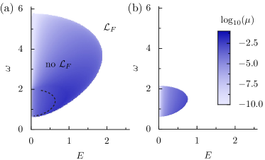
Figure 1: Distance to Markovianity $\mu_{\mathrm{min}}$ of the Floquet generator $\mathcal{K}$ obtained from the one-cycle evolution superoperator as a function of driving strength $E$ and frequency $\omega$, for weak dissipation $\gamma=0.01$ and two driving phases (a) $\varphi=0$ and (b) $\varphi=\pi/2$. In the white region, where $\mu_{\text{min}}=0$, it is of Lindblad type, so that a Floquet Lindbladian $\mathcal{L}_{F}$ exists. On the dashed line the Floquet map $\mathcal{P}(T)$ pair of eigenvalues coincide when crossing the negative real semi-axis.

To illustrate the problem, we consider a driven two-level system described by the master equation $\partial_{\tau}\varrho(\tau)=\mathcal{L}(\tau)\varrho(\tau)$ with time-periodic Lindbladian generator $\mathcal{L}(\tau)=-{i}[H(\tau),\cdot]+\kappa\,\left(\sigma_{-}\cdot\sigma_{+}-\frac{1}{2}\{\sigma_{+}\sigma_{-},\cdot\}\right),$ with $H(\tau)=\frac{\Delta}{2}\sigma_{z}+\mathcal{E}\cos(\Omega\tau-\varphi)\,\sigma_{x}.$ Here $\sigma_{x}$, $\sigma_{z}$, and $\sigma_{-}$ are standard Pauli and lowering operators. After introducing $t=\tau\Delta$, i.e. using $1/\Delta$ as unit for time, we find $\partial_{t}\varrho(t)=\mathcal{L}(t)\varrho(t)$ with

$$\mathcal{L}(t)=-{i}[H(t),\cdot]+\gamma\,\left(\sigma_{-}\cdot\sigma_{+}-\frac{1}{2}\{\sigma_{+}\sigma_{-},\cdot\}\right),$$ (14)

and

$$H(t)=\frac{1}{2}\sigma_{z}+{E}\cos(\omega t-\varphi)\,\sigma_{x}.$$ (15)

This model is characterized by four dimensionless parameters: the relative dissipation strength $\gamma=\kappa/\Delta$ as well as the relative strength $E=\mathcal{E}/\Delta$, frequency $\omega=\Omega/\Delta$ and phase $\varphi$ of the driving.

In Fig. 1 we present the distance from Markovianity for the effective time-independent Floquet generator of our model, obtained using the procedure described in the previous section. Note that the spectrum of a CPTP map is invariant under complex conjugation. Thus for the two-level system we have at most one pair of complex eigenvalues and, therefore, have to check a single integer $x$ labelling the branches of the operator logarithm. If we find a branch $x_{0}$ with a generator of the Lindblad form, then this would be our Floquet Lindbladian $\mathcal{L}_{F}=\mathcal{K}_{x_{0}}$. In Fig. 1(a), we mark the region where such a branch was found and therefore the Floquet Lindbladian exists with white color. In the region where no such branch exists, we plot the distance from Markovianity $\mu_{\text{min}}$ for the closest branch. For weak dissipation $\gamma=0.01$ and $\varphi=0$, an extended non-Lindbladian phase is surrounded by a Lindbladian phase (white region) where $\mu_{\text{min}}=0$ so that $\mathcal{L}_{F}$ can be constructed.

For sufficiently large and small driving frequencies $\omega$ as well as for zero driving ($E=0$) and in the regime of strong driving amplitudes $E$, a Floquet Lindbladian is found to exist. Only for intermediate driving frequencies $\omega$ and sufficiently small (but finite) driving strengths $E$, a lobe-shaped region exists, where the Floquet generator is not markovian, i.e. not of Lindblad-type.

Figure 1(b) shows the phase diagram for another driving phase, $\varphi=\pi/2$. Remarkably, compared to $\varphi=0$, Fig. 1(a), the non-Lindbladian phase covers now a much smaller region of the parameter space. In Fig. 2 we plot the same phase diagram again, but for multiple intermediate values of the driving phase $\varphi$ and observe how the non-Lindbladian region continuously changes its shape with driving phase and appears to be smallest for $\varphi=\pi/2$. The phase boundaries therefore depend on the driving phase or, in other words, on when during the driving period we monitor the stroboscopic evolution of the system.

In the coherent case ($\gamma=0$ for our model), we can decompose the time evolution operator of a Floquet system from time $t_{0}$ to time $t$ like (see, e.g., Ref. Eckardt and Anisimovas (2015))

$$U(t,t_{0})=U_{F}(t)\exp[-i(t-t_{0})H_{\text{eff}}]U_{F}^{\dagger}(t_{0}),$$ (16)

where $U_{F}(t)=U(t+T)$ is a unitary operator describing the time-periodic micromotion of the Floquet states of the system and $H_{\text{eff}}$ is a time-independent effective Hamiltonian. The Floquet Hamiltonian $H^{F}_{t_{0}}$, defined via $U(t_{0}+T,t_{0})=\exp(-iTH^{F}_{t_{0}})$ so that it describes the stroboscopic evolution of the system at times $t_{0}$, $t_{0}+T$, …, is for general $t_{0}$ then given by (see, e.g., Ref. Eckardt and Anisimovas (2015))

$$H^{F}_{t_{0}}=U_{F}(t_{0})H_{\text{eff}}U_{F}^{\dagger}(t_{0}).$$ (17)

Thus the operator $H^{F}_{t_{0}}$ depends on the micromotion via a $t_{0}$-dependent unitary rotation. However, in the dissipative system the micromotion will no longer be captured with a unitary operator. This explains why the effective time-independent generator of the stroboscopic evolution can change its character in a nontrivial fashion, e.g. from Lindbladian to non-Lindbladian form, as a function of $t_{0}$ (or, equivalently, of the driving phase $\varphi$). In Sec. VI, we will present strong evidence for the fact that the breakdown of ‘Lindbladianity’ of the Floquet generator is entirely due to the impact of the micromotion operator.

(a) $\varphi=0.1\pi$

(b) $\varphi=0.2\pi$

(c) $\varphi=0.3\pi$

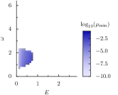
(d) $\varphi=0.4\pi$

Figure 2: Distance to Markovianity $\mu_{\mathrm{min}}$ for different values of the driving phase $\varphi$. Other parameters are as in Fig. 1.

The fact that the Floquet generator for the stroboscopic evolution $\mathcal{K}$ is found to be of Lindblad form in the high-frequency regime (Fig. 1), suggests that it is possible to analytically approximate this Floquet Lindbladian by using systematic high-frequency expansions. However, in the literature it was found that one of the most conventional high-frequency expansions, the Magnus expansion Blanes et al. (2009), generally does not produce a valid Lindblad generator Reimer et al. (2018); Haddadfarshi et al. (2015). Below, in Sec. IV we show that this is also the case, when directly applying the Magnus expansion to our model (14). We will then show how a high-frequency expansion that is consistent with the phase diagrams of Fig. 1 can still be obtained by conducting it in a suitably chosen rotating frame. In the rotating frame, it even explains the transition to the non-Lindbladian phase as a consequence of the non-unitary micromotion, when the frequency is lowered.

III High-frequency expansions and extended Floquet space for open quantum systems

A standard tool to extract the Floquet Hamiltonian in the high-frequency limit is the Magnus expansion Blanes et al. (2009). In line with what has been developed in the literature Reimer et al. (2018); Haddadfarshi et al. (2015) we apply the Magnus expansion to the special case of a time-periodic Lindblad superoperator. For a two-level system it takes the general form

$$\mathcal{L}(H,{d})=-i\left[H,\cdot\right]+\sum_{n,m}d_{nm}\,\left(\sigma_{n}\cdot\sigma_{m}-\frac{1}{2}\left\{\sigma_{m}\sigma_{n},\cdot\right\}\right),$$ (18)

with traceless Hamiltonian $H$ governing the coherent evolution and Kossakowski matrix ${d}$ governing the dissipative component of the evolution. Recall that for the evolution to be physical, i.e. completely positive and trace-preserving, the Kossakowski matrix has to be positive semi-definite, ${d}\geqslant 0$. With this notation, commutators of Lindblad superoperators can be evaluated by using the general expressions for the commutators of two general two-level system Lindblad superoperators (see Appendix D).

As an alternative approach to compute the Floquet generator of an open system, we will also work out a non-Hermitian version of van-Vleck degenerate perturbation theory in the Floquet space of time-periodic density matrices. This extended Floquet state space is given by the product space of the original state space of density matrices with that of time-periodic functions. This approach is a generalisation of the method described in Ref. Eckardt and Anisimovas (2015) for isolated driven quantum systems. It has the advantage that it clearly isolates the effect of the micromotion. Namely, it gives rise to an effective generator that is independent of the driving phase. Combining this object with a driving-phase dependent micromotion operator, then provides the Floquet generator for the stroboscopic evolution.

III.1 The Magnus expansion

Because the Lindblad superoperator is time periodic, we can expand it in the Fourier series,

$$\mathcal{L}(t) =\sum_{n\in\mathbb{Z}}e^{i\omega nt}\mathcal{L}_{n}.$$ (19)

The Magnus expansion Blanes et al. (2009) is a general high-frequency expansion for linear differential equations with periodic coefficients. Therefore it can be directly applied to our problem. It gives rise to one candidate $\mathcal{K}$ for $\mathcal{L}_{F}$. Let us denote this expansion of the generator by

$$\mathcal{K}_{\mathrm{Mag}} =\sum_{n=1}^{\infty}\mathcal{K}^{(n)},$$ (20)

which we approximate by truncating the series after some order $k$, giving

$$\mathcal{K}_{\mathrm{Mag,k}} =\sum_{n=1}^{k}\mathcal{K}^{(n)}.$$ (21)

The leading coefficients read

$$\mathcal{K}^{(1)} =\frac{1}{T}\int_{0}^{T}\mathrm{d}t\mathcal{L}(t)=\mathcal{L}_{0}$$ (22)

$$\mathcal{K}^{(2)} =\frac{1}{2T}\int_{0}^{T}\mathrm{d}t\int_{0}^{t}\mathrm{d}t^{\prime}\left[\mathcal{L}(t),\mathcal{L}(t^{\prime})\right]$$ (23)

$$=i\sum_{n=1}^{\infty}\frac{\left[\mathcal{L}_{n},\mathcal{L}_{-n}\right]+\left[\mathcal{L}_{0},\mathcal{L}_{n}-\mathcal{L}_{-n}\right]}{n\omega},$$ (24)

$$\begin{split}\mathcal{K}^{(3)}&=\frac{1}{6T}\int_{0}^{T}\mathrm{d}t\int_{0}^{t}\mathrm{d}t^{\prime}\int_{0}^{t^{\prime}}\mathrm{d}t^{\prime\prime}\bigl{(}\left[\mathcal{L}(t),\left[\mathcal{L}(t^{\prime}),\mathcal{L}(t^{\prime\prime})\right]\right]\\ &\qquad\qquad+\left[\mathcal{L}(t^{\prime\prime}),\left[\mathcal{L}(t^{\prime}),\mathcal{L}(t)\right]\right]\bigr{)}.\end{split}$$ (25)

For an expression of the third-order contribution in terms of the Fourier components of $\mathcal{L}(t)$ see Appendix B.

III.2 Floquet space

Since $\mathcal{L}(t)$ is periodic, we can apply Floquet’s theorem to Eq. (1) and find that the fundamental solutions of Eq. (1) are Floquet states of the form

$$\varrho_{a}(t)=e^{-i\Omega_{a}t}\,\Phi_{a}(t)$$ (26)

where index $a$ runs over all $N^{2}$ fundamental solutions, with complex numbers $\Omega_{a}$ (replacing the quasienergies in the case of an isolated system) and time-periodic operators $\Phi_{a}(t)=\Phi_{a}(t+T)$ (replacing the Floquet modes). Note that the representation in Eq. (26) is not unique, namely by setting

$$\Omega_{a} \longrightarrow\Omega_{a}+m\omega,\qquad m\in\mathbb{Z}$$ (27)

$$\Phi_{a}(t) \longrightarrow\mathrm{e}^{im\omega t}\Phi_{a}(t)$$ (28)

we could find an equivalent representation of Eq. (26), that will later appear as a (seemingly) independent solution in the Floquet space formalism.

We can expand the time-periodic operators $\Phi_{a}$ in a Fourier series

$$\Phi_{a}(t) =\sum_{n\in\mathbb{Z}}e^{i\omega nt}\,\Phi_{a,n}.$$ (29)

Plugging both Fourier expansions, Eq. (19) and Eq. (29), into Eq. (1), we find

$$\sum_{n}(-i\Omega_{a}+i\omega n)\,\Phi_{a,n}e^{i\omega nt}=\sum_{k,m}\mathcal{L}_{k}\Phi_{a,m}\,e^{i\omega(k+m)t}.$$ (30)

Recall that the $\mathcal{L}_{n}$ are superoperators that act on the $\Phi_{a,n}$, which are linear operators on $\mathcal{H}$, $\Phi_{a,n}\in L(\mathcal{H})$.

By comparing the prefactors of the exponential functions, we find an eigenvalue equation in the ‘extended’ Hilbert space $L(\mathcal{H})\otimes\mathcal{T}$, where $\mathcal{T}$ shall denote the space of time-periodic functions with period $T$. It reads

$$\Omega_{a}\Phi_{a,n}=\sum_{m}(i\mathcal{L}_{n-m}+\delta_{nm}\,m\omega\,\mathbf{1})\,\Phi_{a,m}=\sum_{m}\bar{\mathcal{Q}}_{nm}\,\Phi_{a,m},$$ (31)

where $\bar{\mathcal{Q}}$ is the extended-space representation of the superoperator,

$$Q(t)=i\mathcal{L}(t)-i\partial_{t}.$$ (32)

This superoperator is the generalization of the quasienergy operator $H(t)-i\partial_{t}$ found for isolated systems to the open system.

Similar to the case of isolated systems, Eq. (31) possesses a transparent block structure

$$\Omega_{a}\begin{pmatrix}\dots\\ {\Phi_{a,-1}}\\ {\Phi_{a,0}}\\ {\Phi_{a,1}}\\ \dots\end{pmatrix}=\begin{pmatrix}\dots&\\ &i\mathcal{L}_{0}-\omega\,\mathbf{1}&i\mathcal{L}_{-1}&i\mathcal{L}_{-2}\\ &i\mathcal{L}_{1}&i\mathcal{L}_{0}&i\mathcal{L}_{-1}\\ &i\mathcal{L}_{2}&i\mathcal{L}_{1}&i\mathcal{L}_{0}+\omega\,\mathbf{1}\\ &&&&\dots\end{pmatrix}\begin{pmatrix}\dots\\ {\Phi_{a,-1}}\\ {\Phi_{a,0}}\\ {\Phi_{a,1}}\\ \dots\end{pmatrix},$$ (33)

however the entries in the vectors are now operators and the entries in the matrix are nonhermitian (but Hermiticity-preserving) superoperators.

III.3 van-Vleck high-frequency expansion

The aim of the van-Vleck high-frequency expansion is to find a rotation $\bar{\mathcal{D}}$ that block diagonalizes the problem in the extended space,

$$\bar{\mathcal{Q}}^{\prime}=\bar{\mathcal{D}}^{-1}\bar{\mathcal{Q}}\bar{\mathcal{D}},$$ (34)

such that

$$\bar{\mathcal{Q}}^{\prime}_{nm}=\delta_{nm}(i\mathcal{K}_{\mathrm{eff}}+\,m\omega\,\mathbf{1}).$$ (35)

This transformation to a block-diagonal form is desired, since Eq. (33) is block diagonal for a time-independent generator. As we will see, this transformation therefore leads into a frame where the dynamics is governed by the time-independent generator $\mathcal{K}_{\mathrm{eff}}$. However, in contrast to the closed system, $\bar{\mathcal{Q}}$ is not necessarily Hermitian, so the rotation $\mathcal{D}$ is in general not a unitary transformation. Still, the spectrum $\Omega_{a}$ is of course invariant under this transformation.

In analogy to the coherent case Eckardt and Anisimovas (2015), it suffices to take into account time-periodic transformations $\mathcal{D}(t)=\sum_{n}e^{i\omega nt}\mathcal{D}_{n}$, therefore in extended space the operator $\bar{\mathcal{D}}_{nm}$ may only depend on the difference of the phonon indices $\bar{\mathcal{D}}_{nm}=\mathcal{D}_{n-m}$. First of all, we observe that for two time-local time-periodic superoperators,

$$\mathcal{A}(t)=\sum_{n\in\mathbb{Z}}e^{i\omega nt}\mathcal{A}_{n}\quad\text{and}\quad\mathcal{B}(t)=\sum_{n\in\mathbb{Z}}e^{i\omega nt}\mathcal{B}_{n},$$ (36)

the product of both operators in the time domain

$$\mathcal{C}(t) =\mathcal{A}(t)\mathcal{B}(t)=\sum_{n,m\in\mathbb{Z}}e^{i\omega(n+m)t}\mathcal{A}_{n}\mathcal{B}_{m}$$ (37)

$$=\sum_{n,m\in\mathbb{Z}}e^{i\omega nt}\mathcal{A}_{n-m}\mathcal{B}_{m},$$ (38)

leads in the extend space to

$$\bar{\mathcal{C}}_{nm} =\mathcal{C}_{n-m}=\sum_{k\in\mathbb{Z}}\mathcal{A}_{n-m-k}\mathcal{B}_{k}$$ (39)

$$=\sum_{k\in\mathbb{Z}}\mathcal{A}_{n-k}\mathcal{B}_{k-m}=(\bar{\mathcal{A}}\bar{\mathcal{B}})_{nm}.$$ (40)

Therefore, products in the time domain directly translate into products in the extended space and vice versa. As a result, the inverse transformation $\bar{\mathcal{D}}^{-1}$ in the extended space is just the representation of the inverse transformation in time,

$$\mathcal{D}^{-1}(t)=\sum_{n}e^{i\omega nt}(\mathcal{D}^{-1})_{n}\quad\text{with}\quad\mathcal{D}^{-1}(t)\mathcal{D}(t)=1,$$ (41)

i.e. we have $(\bar{\mathcal{D}}^{-1})_{nm}=(\mathcal{D}^{-1})_{n-m}$.

Thus, the transformation in Eq. (34) becomes $\Phi_{a}^{\prime}(t)={\mathcal{D}}^{-1}(t)\Phi_{a}(t)$, and therefore $\varrho^{\prime}(t)={\mathcal{D}}^{-1}(t)\varrho(t)$. The equation of motion in the transformed frame reads

$$\partial_{t}{\varrho}^{\prime}(t) =(\partial_{t}\mathcal{D}^{-1}(t))\varrho(t)+\mathcal{D}^{-1}(t)\partial_{t}\varrho(t)$$

$$\equiv{\mathcal{L}}^{\prime}(t){\varrho}^{\prime}(t)$$ (42)

Thus, much like to the coherent case, this transformation is equivalent to

$${\mathcal{L}}^{\prime}(t)[\cdot] =(\partial_{t}\mathcal{D}^{-1}(t))\mathcal{D}(t)\cdot+\mathcal{D}^{-1}(t)\mathcal{L}(t)[\mathcal{D}(t)\cdot].$$ (43)

resembling a gauge transformation.

As pointed out already in the literature Dai et al. (2017) and in analogy to the closed system, Eq. (16), the effective generator $\mathcal{K}_{\text{eff}}$ appearing in Eq. (35) fulfills

$$\mathcal{P}(t,t_{0})=\mathcal{D}(t)\exp[(t-t_{0})\mathcal{K}_{\text{eff}}]\mathcal{D}^{-1}(t_{0}).$$ (44)

It is the time-independent generator describing the evolution in a “rotating frame of reference”. However, since the dynamics is dissipative, the time-periodic “micromotion” operator $\mathcal{D}(t)$ that describes this transformation, is generally not unitary anymore. Defining a general Floquet generator $\mathcal{K}_{t_{0}}$ via

$$\mathcal{P}(t_{0}+T,t_{0})=\exp\left(\mathcal{K}_{t_{0}}T\right),$$ (45)

so that $\mathcal{K}=\mathcal{K}_{0}$ corresponds to the Floquet generator defined by Eq. (9) for the case of $t_{0}=0$, it can be expressed in terms of the effective generator $\mathcal{K}_{\text{eff}}$ and the micromotion operator $\mathcal{D}(t)$,

$$\mathcal{K}_{t_{0}}=\mathcal{D}(T+t_{0})\mathcal{K}_{\text{eff}}\mathcal{D}^{-1}(t_{0}).$$ (46)

Since the micromotion superoperator $\mathcal{D}(t_{0})$ is generically non-unitary, it is possible that it maps a Lindbladian effective generator $\mathcal{K}$ to a non-Lindbladian Floquet generator $\mathcal{K}_{t_{0}}$. This explains the driving-phase dependence (which is equivalent to a dependence on $t_{0}$) observed in Fig.  1. Moreover, below we find strong evidence suggesting that $\mathcal{K}_{\text{eff}}$ is always of Lindblad type, so that the non-Markovianity of $\mathcal{K_{t_{0}}}$, as it is found in the non-Lindbladian lobes of Fig. 1, must entirely entirely be to the micromotion captured by $\mathcal{D}(t_{0})$.

In Ref. Dai et al. (2017) a high-frequency expansion for both the effective generator $\mathcal{K}_{\mathrm{eff}}$ and the micromotion superoperator $\mathcal{D}(t)$ were derived. Here we present an alternative derivation of such a high-frequency expansion by applying van-Vleck-type degenerate perturbation theory the extended Floquet space. Genealizing the reasoning of Ref. Eckardt and Anisimovas (2015) to the non-Hermitian problem of the open system, we decompose $\mathcal{Q}$ into an unperturbed blockdiagonal part $\bar{\mathcal{Q}}_{0}$ and a perturbation $\bar{\mathcal{V}}$ that can also contain block-off-diagonal terms,

$$\bar{\mathcal{Q}}=\bar{\mathcal{Q}}_{0}+\lambda\bar{\mathcal{V}},$$ (47)

with $(\bar{\mathcal{Q}}_{0})_{nm}=\delta_{nm}m\omega\mathbf{1}$. Applying van Vleck perturbation theory, we obtain (Appendix C)

$$\mathcal{K}_{\text{eff}} = \sum_{n=1}^{\infty}\mathcal{K}^{(n)}_{\text{eff}}$$ (48)

$$\mathcal{D}(t) = \exp(\mathcal{G}(t))\quad\text{ with }\quad\mathcal{G}(t)=\sum_{n=1}^{\infty}\mathcal{G}^{(n)}(t),$$ (49)

where (see also Dai et al. (2017))

$$\mathcal{K}^{(1)}_{\text{eff}} =\mathcal{L}_{0},$$ (50)

$$\mathcal{K}^{(2)}_{\text{eff}} =i\sum_{n=1}^{\infty}\frac{\left[\mathcal{L}_{n},\mathcal{L}_{-n}\right]}{n\omega},$$ (51)

$$\mathcal{K}^{(3)}_{\text{eff}} =-\sum_{n\neq 0}\left(\frac{\left[\mathcal{L}_{n},\left[\mathcal{L}_{0},\mathcal{L}_{-n}\right]\right]}{2n^{2}\omega^{2}}+\sum_{\begin{subarray}{c}m\neq 0,\\ m\neq n\end{subarray}}\frac{\left[\mathcal{L}_{m},\left[\mathcal{L}_{n-m},\mathcal{L}_{-n}\right]\right]}{3nm\omega^{2}}\right).$$ (52)

and

$$\mathcal{G}^{(1)}(t) =-i\sum_{n\neq 0}e^{in\omega t}\frac{\mathcal{L}_{n}}{n\omega},$$ (53)

$$\mathcal{G}^{(2)}(t) =-\sum_{n\neq 0}e^{in\omega t}\left(\frac{\left[\mathcal{L}_{0},\mathcal{L}_{n}\right]}{n^{2}\omega^{2}}+\sum_{\begin{subarray}{c}m\neq 0,\\ m\neq n\end{subarray}}\frac{\left[\mathcal{L}_{n-m},\mathcal{L}_{m}\right]}{2mn\omega^{2}}\right).$$ (54)

These expressions take exactly the same structure as those found for isolated systems Eckardt and Anisimovas (2015).

IV High-frequency expansion: Direct frame

Let us now apply both types of high-frequency expansion described in the previous section to our model system. Although a Lindblad-type Floquet generator is found numerically to exist in the high-frequency regime, this behaviour is not reproduced by both the Magnus and the van-Vleck-type expansion when directly applied to the model (14).

IV.1 Emergence of non-Lindbladian terms in the Magnus expansion

Let us compute the leading terms of the Magnus expansion for the effective Floquet generator for the two-level system defined in Eq. (14) with driving phase $\varphi=0$. The Fourier-expansion of our model yields three non-vanishing terms,

$$\mathcal{L}_{0} =-i\left[\frac{\sigma_{z}}{2},\cdot\right]+\gamma\,\left(\sigma_{-}\cdot\sigma_{+}-\frac{1}{2}\{\sigma_{+}\sigma_{-},\cdot\}\right)$$ (55)

and

$$\mathcal{L}_{1} =\mathcal{L}_{-1}=-i\frac{E}{2}\left[\sigma_{x},\cdot\right].$$ (56)

The second order of the expansion drops out, $\mathcal{K}^{(2)}=0$, (as well as all other even orders). Using Eq. (25), up to the third order we, therefore, find

$$\mathcal{K}_{\mathrm{Mag,3}}=\mathcal{L}_{0}+\frac{2}{\omega^{2}}\left[\mathcal{L}_{0},\left[\mathcal{L}_{0},\mathcal{L}_{1}\right]\right]-\frac{1}{\omega^{2}}\left[\mathcal{L}_{1},\left[\mathcal{L}_{0},\mathcal{L}_{1}\right]\right].$$ (57)

By using the general expressions for the commutator of two general two-level system Lindblad superoperators that we present in Appendix D, we compute

$$\left[\mathcal{L}_{0},\mathcal{L}_{1}\right]=\mathcal{L}(H_{a},{d_{a}}),$$ (58)

with

$$\text{ with }H_{a}=\frac{E}{2}\sigma_{y}\quad\text{ and }\quad d_{a}=\gamma E\begin{pmatrix}0&0&-i\\ 0&0&-1\\ i&-1&0\end{pmatrix},$$ (59)

where $\mathcal{L}(H,{d})$ is defined in Eq. (18). Similarly, we find

$$\left[\mathcal{L}_{0},\left[\mathcal{L}_{0},\mathcal{L}_{1}\right]\right]=\mathcal{L}(H_{b},{d}_{b}),$$ (60)

with

$$H_{b}=-\frac{E}{2}\sigma_{x}\quad\text{ and }\quad{d}_{b}=2\gamma E\begin{pmatrix}0&0&1\\ 0&0&-i\\ 1&i&0\end{pmatrix},$$ (61)

as well as

$$\left[\mathcal{L}_{1},\left[\mathcal{L}_{0},\mathcal{L}_{1}\right]\right]=\mathcal{L}(H_{c},{d}_{c}),$$ (62)

with

$$H_{c}=\frac{E^{2}}{2}\sigma_{z}+\mathcal{O}(\gamma^{2})\text{ and }{d}_{c}=\gamma E^{2}\begin{pmatrix}0&i&0\\ -i&2&0\\ 0&0&-2\end{pmatrix}+\mathcal{O}(\gamma^{2}).$$ (63)

Altogether, in third order Magnus expansion (and first order in $\gamma$), the Floquet generator is approximated by

$$\mathcal{K}_{\mathrm{Mag,3}} =\mathcal{L}(H_{\mathrm{Mag,3}},{d}_{\mathrm{Mag,3}}),$$ (64)

with

$$H_{\mathrm{Mag,3}}=-\frac{\varepsilon}{\omega}\sigma_{x}+\frac{1}{2}\left(1-\varepsilon^{2}\right)\sigma_{z}$$ (65)

and

$${d}_{\mathrm{Mag,3}}=\gamma\begin{pmatrix}1&i(1-\varepsilon^{2})&4\varepsilon/\omega\\ -i(1-\varepsilon^{2})&1-2\varepsilon^{2}&-4i\varepsilon/\omega\\ 4\varepsilon/\omega&4i\varepsilon/\omega&2\varepsilon^{2}\end{pmatrix},$$ (66)

where $\varepsilon={E}/{\omega}$.

The matrix distance of the matrix representation of the superoperator $\mathcal{K}_{\mathrm{Mag,3}}$ to the matrix representation of the exact Floquet generator $\mathcal{K}$ is shown in Fig. 3(a). Note that although for high frequencies, $\omega\to\infty$, this distance approaches zero, for any finite $\gamma\neq 0$ the generator $\mathcal{K}_{\mathrm{Mag,3}}$ is not a valid Lindbladian generator in the whole region of the parameters. This can be seen from the characteristic polynomial of its dissipator matrix ${d}_{\mathrm{Mag,3}}$, which apart from the prefactor $\gamma$ reads

$$f(\lambda) =\mathrm{det}({d_{\mathrm{Mag,3}}}/\gamma-\lambda\mathbf{1})$$ (67)

$$=-\lambda^{3}+2\lambda^{2}-\lambda\left(4\varepsilon^{2}-5\varepsilon^{4}-\frac{32\varepsilon^{2}}{\omega^{2}}\right)-2\varepsilon^{6}.$$ (68)

As illustrated in Fig. 3(b), for $\lambda\rightarrow-\infty$ we have $f(\lambda)\rightarrow\infty$, but at the same time one finds $f(0)=-2\varepsilon^{6}<0$. Therefore there will always be a negative eigenvalue $\lambda$ and the Kossakowski matrix ${d}_{\mathrm{Mag,3}}$ is not positive semi-definite. As a result, the third-order Magnus approximation of the Floquet generator $\mathcal{K}_{\mathrm{Mag,3}}$ is not of Lindblad form. This is unsatisfactory, since the Floquet generator has been shown to be of Lindblad form numerically in the limit of large driving frequencies.

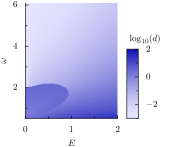
(a)

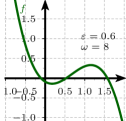
(b)

Figure 3: (a) Distance (the Frobenius norm) $d=||\mathcal{K}_{\mathrm{Mag,3}}-\mathcal{K}_{x_{0}}||_{F}$ between the generator $\mathcal{K}_{\mathrm{Mag,3}}$ obtained with the third-order Magnus expansion in the direct frame and the exact generator $\mathcal{K}_{x_{0}}\in\mathrm{log}(\mathcal{P}(T))/T$ from branch closest to a Lindblad generator. (b) Typical graph $f(\lambda)$ of the characteristic polynomial of matrix ${d}_{\mathrm{Mag,3}}/\gamma$ of the third order Magnus expansion $\mathcal{K}_{\mathrm{Mag,3}}$ of the Floquet generator. The matrix ${d}_{\mathrm{Mag,3}}$ therefore has one negative eigenvalue for all parameters $\varepsilon,\omega$ and $\gamma>0$.

As was already pointed out in the literature Haddadfarshi et al. (2015), the negative eigenvalue emerges due to the fact that the characteristic polynomial has terms that are of higher order than $1/\omega^{2}$ up to which the Magnus expansion was performed. It is indeed expected, that the characteristic polynomial is correct only up to this order,

$$f(\lambda)=-\lambda^{3}+2\lambda^{2}-4\varepsilon^{2}\lambda,$$ (69)

and that the next higher order will only be revealed after evaluating the Magnus expansion up to fourth order and so on. Note that if we only take into account the terms up to order $1/\omega^{2}$, Eq. (69), indeed, the characteristic polynomial only has nonnegative eigenvalues, so one could argue that complete positivity is only violated in orders higher than $1/\omega^{2}$. However, if one would want to find a generator that is a valid Lindbladian in this order $1/\omega^{2}$, there is no well-defined procedure on how to modify the terms in the dissipator matrix ${d}$, such that its characteristic polynomial is exactly the one in Eq. (69).

The problem of an non-Lindbladian generator $\mathcal{K}_{\mathrm{Mag}}$ is not originating from a wrong choice of branch for $\mathcal{K}_{\mathrm{Mag}}$. We have also checked the other branches of $\mathcal{K}_{\mathrm{Mag}}$ numerically and they also do not yield a valid Lindbladian generator. In the high-frequency limit $\omega\to\infty$, we generally expect that it suffices to investigate the principal branch. This is because for the high-frequency expansion $\mathcal{K}_{\mathrm{Mag}}(\omega)$ one has (cf. Appendix A)

$$\mathcal{K}_{\mathrm{Mag},\mathbf{x}}(\omega)=\mathcal{K}_{\mathrm{Mag}}(\omega)+i\omega\sum_{c=1}^{n_{c}}x_{c}\left(P_{c}(\omega)-P_{c*}(\omega)\right).$$ (70)

In the high-frequency limit, the principal branch $\mathcal{K}_{\mathrm{Mag}}(\omega)$ converges to the diabatic (or rotating-wave) Lindbladian $\mathcal{K}_{\mathrm{Mag}}(\omega)\rightarrow\mathcal{L}_{0}$, therefore all the projectors will also converge, $P_{c}(\omega)\rightarrow P_{c}(\infty)$. As long as

$$\Phi_{\perp}(P_{c}(\infty)-P_{c*}(\infty))^{\Gamma}\Phi_{\perp}\neq 0$$ (71)

the matrices $V_{c}$ in the Markovianity test, Eq. (162), will scale linearly with $\omega$ in that limit. Therefore, for $\omega\to\infty$ all matrices $V_{\mathbf{x}}(\omega)$ for branches different from $\mathbf{x}=0$ will diverge, leaving only the principal branch as a candidate.

IV.2 Non-Lindbladian terms in the van-Vleck high-frequency expansion

Let us now investigate the effective generator $\mathcal{K}_{\text{eff}}$ using the van-Vleck high-frequency expansion. Since again the second order vanishes, it provides in third-order high-frequency approximation and first order with respect to $\gamma$

$$\mathcal{K}_{\mathrm{eff},3}=\mathcal{L}_{0}-\frac{1}{\omega^{2}}\left[\mathcal{L}_{1},\left[\mathcal{L}_{0},\mathcal{L}_{1}\right]\right].$$ (72)

Employing Eq. (63), we obtain

$$\mathcal{K}_{\mathrm{eff,3}}=\mathcal{L}(H_{\mathrm{eff,3}},{d}_{\mathrm{eff,3}}),$$ (73)

with

$$H_{\mathrm{eff,3}}=\frac{1}{2}\left(1-\varepsilon^{2}\right)\sigma_{z},$$ (74)

and

$${d}_{\mathrm{eff,3}}=\gamma\begin{pmatrix}1&i(1-\varepsilon^{2})&0\\ -i(1-\varepsilon^{2})&1-2\varepsilon^{2}&0\\ 0&0&2\varepsilon^{2}\end{pmatrix}.$$ (75)

Here we may directly read off one eigenvalue of ${d}_{\mathrm{eff,3}}/\gamma$

$$\lambda_{3}=2\varepsilon^{2}.$$ (76)

The other eigenvalues follow from solving

$$0=\tilde{f}(\lambda)=\lambda^{2}-2(1-\varepsilon^{2})\lambda-\varepsilon^{4}.$$ (77)

Again, $\tilde{f}(0)=-\varepsilon^{4}<0$ while asymptotically $\tilde{f}$ is positive, therefore there must be one negative eigenvalue, and also the effective generator is non-Lindbladian. Thus, the van-Vleck high-frequency expansion shares the problems of the Magnus expansion that it does not provide an effective generator of Lindblad form in the high-frequency limit.

V Rotating frame of reference

When considering Floquet engineering in the high-frequency limit, we know from isolated systems that often the regime of strong driving, with the driving amplitude comparable to $\omega$ (which is large compared to other relevant system parameters), is of special interest, since here the driving leads to a noticeable modification of the system properties. A prominent example is coherent destruction of tunneling Grossmann et al. (1991); Eckardt et al. (2005, 2009), occurring when the amplitude of the energy modulation between two tunnel-coupled states is equal to about $2.4\omega$. To, nevertheless, be able to treat this regime using high-frequency expansions, typically a gauge transformation to a rotating frame of reference is performed, before conducting the high-frequency expansion. This frame is defined so that it integrates out the strong driving term, corresponding to the transition to the interaction picture with the driving term playing the role of the unperturbed Hamiltonian. Comparing the results of a high-frequency expansion in the original frame with those obtained in the rotating frame, the terms of the latter correspond to a partial resummation of infinitely many terms of the previous. Namely, while in the original frame, the $n$th order contains powers of the driving amplitude $\leq n$, each order of the rotating-frame expansion can contain arbitrary powers of the driving amplitude. The rotating frame expansion is, thus, non-perturbative with respect to the driving amplitude.

We will now perform such a transformation to a rotating frame also for the open quantum system. However, differently from the case of isolated systems, it will now not only improve the convergence properties of the high-frequency expansion for strong driving. Rather remarkably, it also ensures that the leading orders of the expansion give rise to approximations to the Floquet generator that can be of Lindblad type. Thus, the problem discussed in the previous section, namely that the Magnus and the van-Vleck expansion do not provide Lindblad-type generators when directly applied to our model system, is cured when conducting the high-frequency expansions in the rotating frame of reference.

V.1 Rotating frame of reference

We decompose the time-dependent Lindbladian into its time-average and a driving term,

$$\mathcal{L}(t)=\mathcal{L}_{0}+\mathcal{L}_{d}(t),$$ (78)

with

$$\mathcal{L}_{d}(t)=\sum_{n\neq 0}e^{in\omega t}\mathcal{L}_{n}.$$ (79)

Let us, for the sake of simplicity, assume that $\mathcal{L}_{d}(t)$ commutes with itself at different times,

$$\left[\mathcal{L}_{d}(t),\mathcal{L}_{d}(t^{\prime})\right]=0,\quad\forall t,t^{\prime},$$ (80)

which is equivalent to $\left[\mathcal{L}_{n},\mathcal{L}_{m}\right]=0$, $\forall n,m\neq 0$. In analogy to the coherent case of isolated systems, we consider the transformation generated by the driving term,

$$\tilde{\varrho}(t)=\Lambda^{-1}(t)\varrho(t),$$ (81)

with

$$\Lambda^{-1}(t)=\exp\left(-\int_{0}^{t}\mathrm{d}t^{\prime}\mathcal{L}_{d}(t^{\prime})\right).$$ (82)

We denote operators in the rotating frame with a tilde. In case that only the coherent part of the Lindbladian (i.e. the Hamiltonian) is driven, $\mathcal{L}_{d}(t)=-i\left[H_{d}(t),\cdot\right]$, this transformation reduces to a unitary rotation of the density matrix,

$$\tilde{\varrho}(t)=U^{\dagger}(t)\varrho(t)U(t),$$ (83)

with

$$U(t)=\exp\left(-i\int_{0}^{t}\mathrm{d}t^{\prime}H_{d}(t^{\prime})\right).$$ (84)

The equation of motion in the rotating frame reads

$$\partial_{t}\tilde{\varrho}(t) =(\partial_{t}\Lambda^{-1}(t))\varrho(t)+\Lambda^{-1}(t)\partial_{t}\varrho(t)\equiv\tilde{\mathcal{L}}(t)\tilde{\varrho}(t)$$ (85)

with gauge-transformed Lindbladian

$$\tilde{\mathcal{L}}(t)[\cdot] =(\partial_{t}\Lambda^{-1}(t))\Lambda(t)\cdot+\Lambda^{-1}(t)\mathcal{L}(t)[\Lambda(t)\cdot].$$ (86)

Now, because $\mathcal{L}_{d}(t)$ commutes with itself at different times, also $\Lambda(t)$ commutes with $\mathcal{L}_{d}(t)$, therefore we find

$$\tilde{\mathcal{L}}(t)[\cdot] =-\mathcal{L}_{d}(t)\cdot+\Lambda^{-1}(t)\mathcal{L}_{d}(t)[\Lambda(t)\cdot]+\Lambda^{-1}(t)\mathcal{L}_{0}[\Lambda(t)\cdot]$$ (87)

$$=\Lambda^{-1}(t)\mathcal{L}_{0}[\Lambda(t)\cdot].$$ (88)

By construction, we have eliminated the driving term, at the expense that the transformed static term has now acquired a periodic time-dependence.

From the time evolution operator in the rotating frame, $\tilde{\mathcal{P}}(t)$ (where here and in the following the initial time of the evolution is always understood to be $t=0$), we can define the Floquet Lindbladian $\tilde{\mathcal{K}}$ in the rotating frame in analogy to Eq. (9),

$$\tilde{\mathcal{P}}(T)=\exp({\tilde{\mathcal{K}}T}).$$ (89)

Since for our choice of the driving term $\mathcal{L}_{d}(t)$, one has $\int_{0}^{\nu T}\mathrm{d}t\mathcal{L}_{d}(t)=0$, $\nu\in\mathbb{N}_{0}$, the transformation $\Lambda(t)$ becomes the identity at stroboscopic times $t=\nu T$. Thus, at stroboscopic times the rest frame and the rotating frame coincide, so that

$$\tilde{\varrho}(\nu T)=\varrho(\nu T)$$ (90)

as well as

$$\tilde{\mathcal{P}}(\nu T)=\mathcal{P}(\nu T).$$ (91)

In particular, one has $\tilde{\mathcal{P}}(T)=\mathcal{P}(T)$, which implies that

$$\tilde{\mathcal{K}}=\mathcal{K}.$$ (92)

Note that this is not true for a general choice of $\mathcal{L}_{d}(t)$, e.g., if $\mathcal{L}_{d}(t)$ does not commute with itself at different times.

V.2 Explicit transformation for our model system

We now work out the transformation to the rotating frame for our model system [Eq. (14)]. Since only the Hamiltonian is driven, the transformation is unitary,

$$\tilde{\varrho}(t)=U^{\dagger}(t)\varrho(t)U(t),$$ (93)

where

$$U(t)=\exp\left(-i\chi(t)\sigma_{x}\right),\quad\text{with}\quad\chi(t)=\frac{E}{\omega}\sin(\omega t).$$ (94)

We again consider driving phase $\varphi=0$ only. We find

$$\begin{split}\tilde{\mathcal{L}}(t)[\cdot]=&-i\left[\frac{1}{2}\tilde{\sigma}_{z}(t),\cdot\right]\\ &+\gamma\,\left(\tilde{\sigma}_{-}(t)\cdot\tilde{\sigma}_{+}(t)-\frac{1}{2}\{\tilde{\sigma}_{+}(t)\tilde{\sigma}_{-}(t),\cdot\}\right).\end{split}$$ (95)

Here the rotated Pauli operators read

$$\begin{split}\tilde{\sigma}_{z}(t)&=U^{\dagger}(t)\sigma_{z}U(t)\\ &=\cos(2\chi(t))\sigma_{z}+\sin(2\chi(t))\sigma_{y},\end{split}$$ (96)

$$\begin{split}\tilde{\sigma}_{\pm}(t)&=U^{\dagger}(t)\sigma_{\pm}U(t)\\ &=\sigma_{x}\pm i\left[\cos(2\chi(t))\sigma_{y}-\sin(2\chi(t))\sigma_{z}\right].\end{split}$$ (97)

In order to perform the high-frequency expansions in the rotating frame, let us now determine the Fourier components of the transformed Lindbladian $\tilde{\mathcal{L}}(t)$, Eq. (95). Using the definition $z=2E/\omega$, we may rewrite the Fourier transform

$$\mathcal{F}_{n}[\cos(2\chi(t))]\equiv\frac{1}{T}\int_{0}^{T}\cos(2\chi(t))e^{-in\omega t}\mathrm{d}t$$ (98)

$$=\frac{1}{T}\int_{0}^{T}\frac{1}{2}\left(e^{iz\sin(\omega t)}+e^{-iz\sin(\omega t)}\right)e^{-in\omega t}\mathrm{d}t$$ (99)

$$=\frac{1}{2}\left[J_{n}(z)+J_{-n}(z)\right]=e_{n}J_{n}(z).$$ (100)

Here $J_{n}(z)$ is the $n$-th Bessel function of the first kind, we have used $J_{-n}(z)=(-1)^{n}J_{n}(z)$ and defined

$$e_{n}=\left\{\begin{array}[]{cc}1,&n\text{ even,}\\ 0,&n\text{ odd,}\end{array}\right.\quad\text{and}\quad o_{n}=\left\{\begin{array}[]{cc}0,&n\text{ even,}\\ 1,&n\text{ odd.}\end{array}\right.$$ (105)

Similarly, we find

$$\mathcal{F}_{n}[\sin(2\chi(t))] =-io_{n}J_{n}(z),$$ (106)

$$\mathcal{F}_{n}[\sin(2\chi(t))\cos(2\chi(t))] =-i\frac{o_{n}}{2}J_{n}(2z),$$ (107)

$$\mathcal{F}_{n}[\cos(2\chi(t))^{2}] =\frac{1}{2}\left[\delta_{n0}+e_{n}J_{n}(2z)\right],$$ (108)

$$\mathcal{F}_{n}[\sin(2\chi(t))^{2}] =\frac{1}{2}\left[\delta_{n0}-e_{n}J_{n}(2z)\right],$$ (109)

so that the Fourier components of the Lindblad generator in the rotating frame read

$$\tilde{\mathcal{L}}_{n} =\mathcal{L}(H_{n},{d}_{n}),$$ (110)

with

$$H_{n}=\frac{J_{n}(z)}{2}\left(e_{n}\sigma_{z}-io_{n}\sigma_{y}\right)$$ (111)

and

$${d}_{n} =\gamma\begin{pmatrix}\delta_{n0}&ie_{n}J_{n}(z)&-o_{n}J_{n}(z)\\ -ie_{n}J_{n}(z)&\frac{\delta_{n0}+e_{n}J_{n}(2z)}{2}&\frac{i}{2}o_{n}J_{n}(2z)\\ o_{n}J_{n}(z)&\frac{i}{2}o_{n}J_{n}(2z)&\frac{\delta_{n0}-e_{n}J_{n}(2z)}{2}\end{pmatrix}.$$ (112)

(Note that each of the individual Fourier-components $\tilde{\mathcal{L}}_{n}$ can be brought to Lindblad form simply by the multiplication with a suitable phase factor.)

VI High-frequency expansion: Rotating frame

Let us now perform both types of high-frequency expansion in the rotating frame of reference.

VI.1 Magnus expansion in the rotating frame

VI.1.1 First order Magnus expansion in the rotating frame

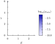
(a)

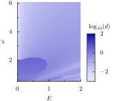
(b)

Figure 4: (a) Distance to Markovianity $\mu_{\mathrm{min}}$ of the Floquet generator $\tilde{\mathcal{K}}_{\mathrm{Mag},1}$($=\tilde{\mathcal{K}}_{\mathrm{eff},1}=\tilde{\mathcal{K}}_{\mathrm{vV},1}$) obtained with the first-order Magnus expansion in the rotating frame for the same model and parameter $\gamma=0.01$ as in Fig. 1(a). The generator is a valid Lindbladian for for all parameters $(E,\omega)$. (b) Distance (the Frobenius norm) $d=||\tilde{\mathcal{K}}-\mathcal{K}_{x_{0}}||_{F}$ between the generator $\tilde{\mathcal{K}}$ obtained by the first-order Magnus expansion $\tilde{\mathcal{K}}_{\mathrm{Mag},1}$ in the rotating frame and the candidate $\mathcal{K}_{x_{0}}\in\mathrm{log}(\mathcal{P}(T))/T$ for the Floquet-Lindbladian $\mathcal{L}_{F}$ of branch ${x_{0}}$, which is closest to the valid Lindbladian generator.

The lowest order of the Magnus expansion in the rotating frame reads

$$\tilde{\mathcal{K}}_{\mathrm{Mag,1}} =\tilde{\mathcal{L}}_{0}=\mathcal{L}(H_{\mathrm{Mag,1}},{d}_{\mathrm{Mag,1}}),$$ (113)

with

$$H_{\mathrm{Mag,1}}=\frac{J_{0}(z)}{2}\sigma_{z}$$ (114)

and

$${d}_{\mathrm{Mag,1}} =\gamma\begin{pmatrix}1&iJ_{0}(z)&0\\ -iJ_{0}(z)&\frac{1}{2}[1+J_{0}(2z)]&0\\ 0&0&\frac{1}{2}[1-J_{0}(2z)]\end{pmatrix}.$$ (115)

where, again, $z=2E/\omega$. Note that for $z\to 0$, i.e. for $E\to 0$ or $\omega\to\infty$ (such that $J_{0}(z)\to 1$) we recover the static Hamiltonian and dissipator, as expected. In Fig. 4(b) we plot the distance of the matrix representation of the superoperator of this approximation $\tilde{\mathcal{K}}$ to the exact Floquet generator and see a much better agreement than what one finds for the lowest order in the direct frame [cf. Fig. 3(a)], especially for smaller values of $\omega$. This is expected because the transformation to the rotating frame integrates out the driving term which corresponds to a partial resummation of infinitely many orders in $E/\omega$, here entering via the nonlinear function Bessel function $J_{0}$. In the direct frame, however, the leading order correction in the Magnus expansion only captures terms up to order $(E/\omega)^{2}$.

The eigenvalues of the coefficient matrix ${d}_{\mathrm{Mag,1}}$ read

$$\lambda_{1/2} =\gamma\left[\mu(z)\pm\sqrt{\mu(z)^{2}+J_{0}(z)^{2}-\frac{1}{2}[1+J_{0}(2z)]}\right],$$ (116)

$$\lambda_{3} =\frac{\gamma}{2}[1-J_{0}(2z)],$$ (117)

with $\mu(z)=[3+J_{0}(2z)]/4$. The corresponding generator is a valid Lindbladian generator only if all three eigenvalues are non-negative. This is generally the case, since

$$J_{0}(z)^{2}-\frac{1}{2}[1+J_{0}(2z)]$$ (118)

$$=J_{0}(z)^{2}-\frac{1}{2}\sum_{k\in\mathbb{Z}}J_{k}(z)^{2}-\frac{1}{2}\sum_{k\in\mathbb{Z}}J_{k}(z)J_{-k}(z)$$ (119)

$$=J_{0}(z)^{2}-\sum_{k\in\mathbb{Z}}J_{2k}(z)^{2}=-\sum_{k\neq 0}J_{2k}(z)^{2}\leq 0,$$ (120)

In the first step we have used the identity $J_{n}(y+z)=\sum_{k\in\mathbb{Z}}J_{k}(y)J_{n-k}(z)$ and that $1=\sum_{k\in\mathbb{Z}}J_{k}(z)^{2}$. This shows that the values that the square root in Eq. (116) takes will be smaller than $\mu(z)$. Therefore, the first order expansion in the rotating frame produces a nontrivial generator $\tilde{\mathcal{K}}_{\mathrm{Mag,1}}$ that is a valid Lindbladian for all parameter values [Fig. 4(a)].

When comparing the result that we obtain in the rotating frame, Eq. (113), to the one that we obtain when directly performing the Magnus expansion, Eq. (64), we find that by expanding the Bessel function to second order, $J_{0}(z)\approx 1-z^{2}/4$, by using $z=2\varepsilon$ we recover the terms $\propto\varepsilon^{2}$ in Eq. (64), while the terms $\propto\varepsilon/\omega$ will be found in the next order of the rotating-frame Magnus expansion.

VI.1.2 Second order Magnus expansion in the rotating frame

The second order term of the rotating-frame Magnus expansion reads

$$\tilde{\mathcal{K}}^{(2)} =i\sum_{n>0}\frac{\left[\tilde{\mathcal{L}}_{n},\tilde{\mathcal{L}}_{-n}\right]+\left[\tilde{\mathcal{L}}_{0},\tilde{\mathcal{L}}_{n}-\tilde{\mathcal{L}}_{-n}\right]}{n\omega}=\sum_{n>0}2o_{n}\frac{\left[\tilde{\mathcal{L}}_{0},i\tilde{\mathcal{L}}_{n}\right]}{n\omega},$$ (121)

where in the second step we have used that for the Fourier components in Eq. (110) we have $\tilde{\mathcal{L}}_{-n}=(-1)^{n}\tilde{\mathcal{L}}_{n}$.

By employing the general expressions derived in Appendix D, we find that for odd $n$

$$\left[\tilde{\mathcal{L}}_{0},i\tilde{\mathcal{L}}_{n}\right]=\mathcal{L}(H_{n},{d}_{n}),$$ (122)

with

$$H_{n}=-\frac{J_{0}(z)J_{n}(z)}{2}\sigma_{x},$$ (123)

and

$$\quad{d}_{n}=\frac{\gamma}{2}\begin{pmatrix}0&0&f_{n}(z)\\ 0&0&-4iJ_{0}(z)J_{n}(z)\\ f_{n}(z)&4iJ_{0}(z)J_{n}(z)&0\end{pmatrix},$$ (124)

where $f_{n}(z)=J_{n}(z)[1+J_{0}(2z)]+J_{n}(2z)J_{0}(z)$. Moreover, we ignored terms of second or higher order in $\gamma$. Thus, up to second order, the Magnus expansion in the rotating frame reads

$$\tilde{\mathcal{K}}_{\mathrm{Mag,2}}=\mathcal{L}(H_{\mathrm{Mag,2}},{d}_{\mathrm{Mag,2}}),$$ (125)

with

$$H_{\mathrm{Mag,2}}=J_{0}(z)\left[\frac{1}{2}\sigma_{z}-{\frac{\nu(z)}{\omega}}\sigma_{x}\right]$$ (126)

and

$${d}_{\mathrm{Mag,2}}=\gamma\begin{pmatrix}1&iJ_{0}(z)&\frac{1}{\omega}[{\nu(z)(1+J_{0}(2z))+J_{0}(z)\nu(2z)}]\\ -iJ_{0}(z)&\frac{1}{2}[1+J_{0}(2z)]&-\frac{4i}{\omega}J_{0}(z)\nu(z)\\ \frac{1}{\omega}[{\nu(z)(1+J_{0}(2z))+J_{0}(z)\nu(2z)}]&\frac{4i}{\omega}J_{0}(z)\nu(z)&\frac{1}{2}[1-J_{0}(2z)]\end{pmatrix},$$ (127)

where we have introduced $\nu(z)=\sum_{n>0}[o_{n}J_{n}(z)/n]$. Since in leading order order $\nu(z)\simeq z/2$, we also recover the terms $\propto\varepsilon/\omega$ in Eq. (64).

In Fig. 5(b) we show the distance of the matrix representation of the superoperator of $\tilde{\mathcal{K}}_{\mathrm{Mag,2}}$ to the exact Floquet generator and see a small improvement compared to the first-order result in Fig. 4(b). However, the distance from Markovianity, which is plotted in Fig. 4(a), acquires qualitatively different behaviour in second order. While the Floquet generator was always Markovian (i.e. of Lindblad form) in first order, in second order we can now distinguish parameter regions, where it is of Lindblad type, from others, where it is not. Remarkably, the map shown in Fig. 5(a) resembles very much the exact phase diagram of Fig. 1(a). Namely, we can clearly observe a lobe-shape region, where the Floquet generator is non-Markovian. While this region is larger than in the exact phase diagram, the transition between Lindbladian and non-Lindbladian Floquet generator is qualitatively captured correctly by the Floquet-Mangus expansion. Only at very low frequencies, where we cannot expect the high-frequency expansion to provide meaningful results, we find as an artifact a thin non-Markovian stripe, which is not present in the exact phase diagram.

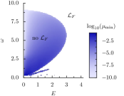
(a)

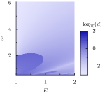
(b)

Figure 5: (a) Distance to Markovianity $\mu_{\mathrm{min}}$ of the Floquet generator $\tilde{\mathcal{K}}_{\mathrm{Mag},2}$ obtained with the second-order Magnus expansion in the rotating frame for the same model and parameter $\gamma=0.01$ as in Fig. 1. Note that we only calculate distances for $\omega\geq 0.3$, values below this are drawn in white. (b) Matrix distance $d$ of the candidate $\tilde{\mathcal{K}}_{\mathrm{Mag},2}$ to the candidate $\mathcal{K}$ obtained from the logarithm of $\mathcal{P}(T)$.

VI.2 Van-Vleck high-frequency expansion in the rotating frame

After having seen that, starting from the rotating frame of reference, the Magnus expansion qualitatively reproduces the exact phase diagram, let us now also evaluate the leading orders of the van-Vleck expansion. Different, however, from the previous section, where we were able to derive analytic expressions for the Magnus expansion, here calculations get quite involved and so we treat this expansion numerically. For this purpose, it is convenient to first discuss the action of the transformation to the rotating frame, $\Lambda(t)$ in the extended Floquet space.

VI.2.1 Floquet-space formalism

Both the rotating-frame transformation $\Lambda(t)$ and the micromotion $\mathcal{D}(t)$ are generalized gauge transformations. Instead of finding $\mathcal{D}(t)$ directly, however, we may first perform a transformation to the rotating frame, $\tilde{\varrho}(t)=\Lambda^{-1}(t)\varrho(t)$, and then find the micromotion transformation there. Since $\Lambda(t)$ is periodic, we have

$$\Lambda(t)=\sum_{n}e^{in\omega t}\Lambda_{n},$$ (128)

so we also may represent it in extended space $\bar{\Lambda}_{nm}=\Lambda_{n-m}$. Note that this representation is only possible since we assume the driving term $\mathcal{L}_{d}(t)$ to commute with itself at different times, so that no time-ordering is needed. As a result $\Lambda(t)$ is a time-local, and thus also time-periodic, superoperator.

As a result, in the rotating frame the generalized quasi-energy operator reads

$$\bar{\tilde{\mathcal{Q}}}=\bar{\Lambda}^{-1}\bar{{\mathcal{Q}}}\bar{\Lambda}.$$ (129)

Like in the direct frame, the goal is to find a transformation $\tilde{\mathcal{D}}$ such that

$$\bar{{\mathcal{Q}}}^{\prime}=\bar{\tilde{\mathcal{D}}}^{-1}\bar{\tilde{\mathcal{Q}}}\bar{\tilde{\mathcal{D}}}$$ (130)

where $\bar{{\mathcal{Q}}}^{\prime}$ is block diagonal.

With respect to the original frame of reference, the micromotion operator is given by the combination

$${\mathcal{D}}(t)=\Lambda(t)\tilde{\mathcal{D}}(t).$$ (131)

From this expression, we can once more directly see that for strong driving the high-frequency expansion in the direct frame will at least have a slow convergence only. Namely, the transformation $\Lambda$ involves a summation of infinitely many terms in $E/\omega$.

In the regular (non-extended) superoperator-space, the rotating-frame quasienergy operator, reads

$$\tilde{\mathcal{Q}}(t)=i\tilde{\mathcal{L}}(t)-i\partial_{t}.$$ (132)

Here the time-periodic Lindbladian generator in the rotating frame, $\tilde{\mathcal{L}}$, is given by Eq. (88). Its Fourier-components $\tilde{\mathcal{L}}_{n}$ are directly related to its Floquet-space representation,

$$\bar{\tilde{\mathcal{L}}}=\bar{\Lambda}^{-1}\bar{{\mathcal{L}_{0}}}\bar{\Lambda}\quad\text{ i.e. }\quad\bar{\tilde{\mathcal{L}}}_{nm}=\tilde{\mathcal{L}}_{n-m}=\sum_{k}\Lambda^{-1}_{n-k}\mathcal{L}_{0}\Lambda_{k-m},$$ (133)

which allows for their efficient numerical calculation. To this end let us determine the coefficients $\Lambda_{n}$. In Appendix F we show that for driving terms of the form

$$\mathcal{L}_{d}(t)=\phi(t)\mathcal{L}_{d}^{\prime},$$ (134)

with scalar function $\phi(t)=\sum_{m\neq 0}e^{im\omega t}\phi_{m}$, one finds the explicit Floquet-space expression:

$$\bar{\Lambda} =\prod_{m\neq 0}\bar{f}^{(m)}\left(\frac{\phi_{m}\mathcal{L}_{d}^{\prime}}{im\omega}\right)\bar{g}^{(m)}\left(\frac{\phi_{m}\mathcal{L}_{d}^{\prime}}{im\omega}\right).$$ (135)

Here we have introduced $\bar{f}^{(m)}_{nl}=f^{(m)}_{n-l}$, $\bar{g}^{(m)}_{nl}=g^{(m)}_{n-l}$ as well as

$$f^{(m)}_{n}(x) =\left\{\begin{array}[]{cc}J_{k}(x)&\text{ if }n=km,k\in\mathbb{Z},\\ 0&\text{ else. }\end{array}\right.$$ (138)

$$g^{(m)}_{n}(x) =\left\{\begin{array}[]{cc}e^{-x}I_{k}(x)&\text{ if }n=km,k\in\mathbb{Z},\\ 0&\text{ else, }\end{array}\right.$$ (141)

with Bessel functions of first kind, $J_{k}$, and modified Bessel functions of first kind, $I_{k}$,. Since $\Lambda^{-1}(t)$ is directly obtained from $\Lambda(t)$ by setting $\phi(t)\rightarrow-\phi(t)$, we find $\bar{\Lambda}^{-1}$ from Eq. (135) by setting $\phi_{m}\rightarrow-\phi_{m}$.

For our example system we have

$$\phi(t)={2}\cos(\omega t),\qquad\mathcal{L}_{d}^{\prime}=\mathcal{L}_{1}=\mathcal{L}_{-1}=-i\left[\frac{E}{2}\sigma_{x},\cdot\right]$$ (142)

From Eq. (135) (or an explicit calculation) we find

$$\Lambda_{n}=J_{n}\left(\frac{2\mathcal{L}_{1}}{i\omega}\right),$$ (143)

which finally yields

$$\tilde{\mathcal{L}}_{n}=\sum_{k}J_{n-k}\left(-\frac{2\mathcal{L}_{1}}{i\omega}\right)\mathcal{L}_{0}J_{k}\left(\frac{2\mathcal{L}_{1}}{i\omega}\right).$$ (144)

By translating superoperators into $N^{2}\times N^{2}$-dimensional matrices as shown in Appendix E, we therefore have an alternative procedure to the one we obtained in Section V.2 to calculate the operators $\tilde{\mathcal{L}}_{n}$ and from this the van-Vleck high-frequency expansion. An explicit calculation of $\tilde{\mathcal{L}}_{n}$ using this matrix representation is given in Appendix G. [Plugging this result into the first order of the Magnus expansion, Eq. (22), one recovers $\tilde{\mathcal{K}}_{\mathrm{Mag,1}}$ of Section VI.1.1.]

Equation (144) is a good starting point for numerical investigations, because it can be evaluated easily, after having represented the superoperators $\mathcal{L}_{0},\mathcal{L}_{1}$ by $N^{2}\times N^{2}$-dimensional matrices. From the expressions in Section III.3 we can then compute the terms of the van-Vleck high-frequency expansion in the rotating frame. We compute both the approximate effective generator, $\tilde{\mathcal{K}}_{\mathrm{eff},n}=\sum_{k=1}^{n}\tilde{\mathcal{K}}_{\mathrm{eff}}^{(k)}$, as well as the approximate micromotion operator $\tilde{\mathcal{D}}_{n}(t)=\exp(\sum_{k=1}^{n}\mathcal{G}_{k}(t))$. Note that for the latter, the expansion of the exponent is truncated, rather than that of the full exponential function. For isolated systems, this makes sure that the micromotion operator is unitary also in finite orders of the approximation Eckardt and Anisimovas (2015). Combining both approximations, we can compute the $n$th order approximation to the Floquet generator

$$\tilde{\mathcal{K}}_{\mathrm{vV},n}=\tilde{\mathcal{D}}_{n-1}(0)\tilde{\mathcal{K}}_{\mathrm{eff},n}\tilde{\mathcal{D}}_{n-1}^{-1}(0).$$ (145)

Here we only need to consider the micromotion correction up to the order of $n-1$, since all terms contained in $\tilde{\mathcal{K}}_{\mathrm{eff},n}$ are of order one or higher. The approximation (145) is generally different from the one obtained from the truncated Magnus expansion in the rotating frame. If, instead, we had expanded and truncated $\tilde{\mathcal{D}}_{n}(t)$ directly, rather than its exponent, we would have recovered the Magnus approximation.

VI.2.2 First order van-Vleck high-frequency expansion in the rotating frame

Note that from comparing Eq. (22) to Eq. (50) we learn that in the leading first order (i.e. zeroth order in $1/\omega$), the van-Vleck high-frequency expansion of the effective generator $\tilde{\mathcal{K}}_{\mathrm{eff}}$ and the Magnus expansion $\tilde{\mathcal{K}}_{\mathrm{Mag}}$ coincide, $\tilde{\mathcal{K}}_{\mathrm{eff,1}}=\tilde{\mathcal{K}}_{\mathrm{Mag,1}}$, therefore in first order also the effective generator exists for all parameter values. Additionally, in leading (zeroth) order the micromotion operator is simply the identiy, $\tilde{\mathcal{D}}_{0}(0)=\mathbf{1}$, so that in leading (first) order, the Floquet generator is equal to the effective generator,

$$\tilde{\mathcal{K}}_{\mathrm{vV},1}=\tilde{\mathcal{K}}_{\mathrm{eff},1}=\tilde{\mathcal{K}}_{\mathrm{Mag,1}}.$$ (146)

Thus, in the rotating frame for the first-order van-Vleck Floquet generator $\tilde{\mathcal{K}}_{\mathrm{vV},1}$ both the distance to Markovianity as well as the distance from the exact Floquet generator are identical to the ones shown in Fig. 4. In particular, $\tilde{\mathcal{K}}_{\mathrm{vV},1}$ is of Lindblad type in the whole parameter plane $(E,\omega)$ [cf. Fig. 4(a)].

VI.2.3 Second order van-Vleck high-frequency expansion in the rotating frame

From the second order on, the truncated van-Vleck expansion for the Floquet generator, $\tilde{\mathcal{K}}_{\mathrm{vV},n}$, deviates both from the effective generator $\tilde{\mathcal{K}}_{\mathrm{eff},n}$ and from the truncated Magnus expansion of the Floquet generator, $\tilde{\mathcal{K}}_{\mathrm{Mag},n}$. However, since for our model we have $\tilde{\mathcal{L}}_{-n}=(-1)^{n}\tilde{\mathcal{L}}_{n}$ and, therefore, $[\tilde{\mathcal{L}}_{n},\tilde{\mathcal{L}}_{-n}]=0$, the second-order contribution to the effective generator vanishes, so that

$$\tilde{\mathcal{K}}_{\mathrm{eff,2}}=\tilde{\mathcal{K}}_{\mathrm{eff,1}}.$$ (147)

Thus, the only new contribution to the Floquet generator

$$\tilde{\mathcal{K}}_{\mathrm{vV},2}=\tilde{\mathcal{D}}_{1}(0)\tilde{\mathcal{K}}_{\mathrm{eff,2}}\tilde{\mathcal{D}}_{1}^{-1}(0)=\tilde{\mathcal{D}}_{1}(0)\tilde{\mathcal{K}}_{\mathrm{eff,1}}\tilde{\mathcal{D}}_{1}^{-1}(0)$$ (148)

stems from the micromoton operator $\tilde{\mathcal{D}}_{1}(0)$.

In Fig. 6, we plot the distance from Markovianity (a) [as well as the distance from the exact Floquet generator for $\tilde{\mathcal{K}}_{\mathrm{vV,2}}$ (b)]. Apart from some artifacts at very low frequencies, we find a lobe-shaped non-Markovian region, where no Floquet-Lindbladian can be found. Thus, like the Magnus expansion, also the van-Vleck expansion explains the structure of the exact phase diagram shown in Fig. 1(a). However, the phase boundaries obtained within the second-order van-Vleck approximation [Fig. 6(a)] are closer to the exact ones [Fig. 1(a)] than those obtained with the Magnus expansion [Fig 4(a)].

Apart from providing a quantitatively better approximation to the exact results, the van-Vleck expansion has another (and more important) advantage compared to the Magnus expansion. Namely, it disentangles effects that result from the micromotion, which are contained in $\tilde{\mathcal{D}}(t_{0})$, from those contained in the $t_{0}$-independent effective generator $\tilde{\mathcal{K}}_{\mathrm{eff}}$. Since $\tilde{\mathcal{K}}_{\mathrm{eff},2}$ is Markovian in the whole parameter plane $(E,\omega)$, we can now clearly see that for our model system the origin of the region with non-Markovian Floquet generator lies (entirely) in the non-unitary micromotion. While this statement is obtained from a second-order high-frequency van-Vleck expansion only, the very good agreement with the exact phase diagram, strongly suggests that this statement remains true also beyond this approximation. This is confirmed also by the third order van-Vleck approximation, which is discussed below. Note that the phase diagram will not be changed further, when transforming from the rotating to the direct frame of reference, because both are related by a unitary transformation for our model system, since the driving term is hermitian.

The relation of regions with non-Markovian Floquet generator with the non-unitary micromotion of the system, is consistent also with the strong dependence of the phase diagram on the driving phase, which is equivalent to a variation of the time $t_{0}$, with $t_{0}=\varphi T/2\pi$. Compare Figs. 1(a) and (b) corresponding to $\varphi=0$ and $\varphi=\pi/2$, respectively or the subfigures of Fig. 2. In order to explain why the non-Markovian lobe in the phase diagram is largest for $\varphi=t_{0}=0$ and shrinks with increasing $\varphi$, until it finds its smallest extent for $\varphi=\pi/2$ or $t_{0}=T/4$, let us inspect the first-order van-Vleck approximation of the micromotion operator (which describes the role of the micromotion in the second-order approximation of the Floquet generator). It reads

$$\tilde{\mathcal{D}}_{1}(t_{0}) =\exp\left(-i\sum_{n\neq 0}e^{in\omega t_{0}}\frac{\tilde{\mathcal{L}}_{n}}{n\omega}\right)$$ (149)

$$=\exp\left(-i\sum_{k=1}^{\infty}2\left[o_{k}\cos(k\omega t_{0})+e_{k}i\sin(k\omega t_{0})\right]\frac{\tilde{\mathcal{L}}_{k}}{k\omega}\right),$$ (150)

where in the second step we have employed that for our model $\tilde{\mathcal{L}}_{-n}=(-1)^{n}\tilde{\mathcal{L}}_{n}$. When the exponent of this expression becomes small, the micromotion operator approaches the identity, which describes a unitary rotation that does not induce any non-Markovian behavior. The largest contribution to the exponent stems from the $k=1$ term, which vanishes precisely when $t_{0}=T/4$ corresponding to the driving phase $\varphi=\pi/2$ at which the non-Markovian region is smallest. Thus, the van-Vleck expansion provides analytical insight into the origin of the phase dependence of the phase diagram.

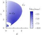
(a)

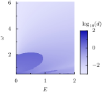
(b)

Figure 6: (a) Distance to Markovianity $\mu_{\mathrm{min}}$ of the Floquet generator ${\mathcal{K}}$ obtained with the second-order van-Vleck high-frequency expansion $\tilde{\mathcal{K}}_{\mathrm{vV},2}$ in the rotating frame, where we do not expand the exponential in $\tilde{\mathcal{D}}(t)=\exp(\tilde{\mathcal{G}}(t))$. We present the same model and parameter $\gamma=0.01$ as in Fig. 1(a). Note that we only calculate distances for $\omega\geq 0.3$, values below this are drawn in white. (b) Distance $d$ of the candidate $\tilde{\mathcal{K}}_{\mathrm{vV},2}$ to the exact candidate $\mathcal{K}$ obtained from the logarithm of $\mathcal{P}(T)$.

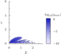
Figure 7: Distance to Markovianity $\mu_{\mathrm{min}}$ of the candidate $\tilde{\mathcal{K}}_{\mathrm{eff},3}$ for the effective generator obtained from a third order van-Vleck high-frequency expansion in the rotating frame for the same model and parameter $\gamma=0.01$ as in Fig. 1. We only calculate for $\omega\geq 0.1$, values below this are drawn in white.

VI.2.4 Third order van-Vleck high-frequency expansion in the rotating frame

In order to support the conclusions drawn from the second-order van-Vleck expansion in the previous section, let us now briefly disucuss the third order. Calculating numerically the effective generator $\tilde{\mathcal{K}}_{\mathrm{eff},3}$, in Figure 7 we show the resulting distance from Markovianity. Apart from artifacts appearing at very small frequencies, $\tilde{\mathcal{K}}_{\mathrm{eff},3}$ is of Lindblad form essentially everywhere in the parameter plane $(E,\omega)$. This confirms that non-Markovian behavior must be an effect of the micromotion.

It is interesting to see that the high-frequency expansion is able to capture the transition between the two phases and it is remarkable that rather good agreement with the exact phase diagram is found also down to quite low frequencies. But for very low frequencies, eventually also qualitative deviations from the exact result become visible. This is not surprising, since the high-frequency expansion cannot be expected to converge in this regime. For the Magnus expansion (and thus also for the van-Vleck expansion), convergence is guaranteed as long as Blanes et al. (2009); Moan and Niesen (2008)

$$\int_{0}^{T}||\mathcal{L}(t)||_{2}\mathrm{d}t<\pi.$$ (151)

Here, $||A||_{2}=\max_{||x||_{2}=1}||Ax||_{2}$ is the induced 2-norm.

We can gain a very rough estimate for the region of convergence by discussing the undriven limit of $E=0$ and $\gamma=0$. As shown in Appendix G, the matrix representation of the generator then reads $\mathcal{L}|_{E=0,\gamma=0}=\mathrm{diag}(0,-i,i,0)$, therefore $||(\mathcal{L}|_{E=0,\gamma=0})||_{2}=1$. Thus, for $E=0$ and $\gamma=0$ we find that the Magnus expansion is only expected to converge for $\omega>2$. For finite values of the driving strength $E$ the norm of $\mathcal{L}(t)$ will increase and thus the radius of convergence will decrease even further.

As a result, Figure 7 shows that within the region of convergence of the Magnus expansion, $\tilde{\mathcal{K}}_{\mathrm{eff},3}$ is a valid Lindbladian. Our hypothesis, that the effective Lindbladian could exist for all parameters, is therefore not violated by the third order of the van-Vleck high-frequency expansion in the rotating frame.

VII Summary and outlook

In this paper, we have studied the description of a time-periodically driven open quantum system using high-frequency expansions (Magnus- or van-Vleck-type). In particular, we have focused on the resulting approximations for the effective time-independent Floquet generator, which is defined so that it describes the stroboscopic evolution of the system in steps of the driving period. Our work is generally motivated by the interesting perspective to apply the concepts of Floquet engineering also to open quantum systems. More specifically, it was initiated by a discrepancy that arose from two observations: On the one hand we found in previous work that the Floquet generator of a simple open periodically driven Markovian two-level system is of Lindblad type in the high-frequency regime Schnell et al. (2020). On the other hand it was pointed out that the Floquet generator resulting from a high-frequency expansion is generally not of Lindblad type Reimer et al. (2018); Haddadfarshi et al. (2015); Mizuta et al. (2021). We have found that high-frequency expansions can correctly describe the behaviour of the system, when applied in a rotating frame of reference. Moreover, by going beyond the leading first order, the high-frequency expansion can even explain the transition to another regime, where the Floquet generator is not of Lindblad type. By isolating the effect of the micromotion within the van Vleck approach, this transition can be attributed entirely to the properties of the non-unitary micromotion of the system, and its dependence on the driving phase can be explained.

Our analysis emphasizes that the approach that some recent works Mizuta et al. (2021) take to argue about the non-existence of a Floquet Lindbladian in an interacting system on the basis of the performance of high-frequency expansions might not be conclusive.

We hope that our results will stimulate further research of periodically driven open quantum systems. Since we focused on a specific model, it is, for instance, a very natural question under what conditions our findings can be generalized to other models. For instance, to the case of non-Markovian completely positive stroboscopic evolution when time-dependent rates $\gamma_{i}(t)$ can become negative  Addis et al. (2014); Siudzińska and Chruściński (2020). Such behaviour may arise from a microscopic derivation of the equation of motion of a (Floquet) system coupled to a heat bath Bastidas et al. (2018); Scopa et al. (2019) and is typically neglected in the Floquet-Born-Markov secular formalism  Kohler et al. (1997); Grifoni and Hänggi (1998). Applying our approach to such microscopically derived master equations is, therefore, another interesting perspective.

Finally, it is an open question, whether the observation that the origin of the non-Markovianity of the Floquet generator lies in the micromotion, which was made here based on a high-frequency expansion of a specific model, generalizes to all or a subclass of time-periodically Markovian quantum systems.

VIII Acknowledgments

S.D. acknowledges support by the Russian Science Foundation through Grant No. 19-72-20086 and A.S. and A.E. by the German Research Foundation (DFG) via the Research Unit FOR 2414 (project No. 277974659). A part of this work is a result of the activity of the MPIPKS Advanced Study Group “Open quantum systems far from equilibrium”.

Appendix A Finding the Floquet generator from the exact map $\mathcal{P}(T)$

Here, we summarize the results of Ref. Schnell et al. (2020) concerning the question of the existence of a Floquet Lindbladian. In the time-periodically modulated isolated system, i.e. in our notation Eq. (1) with $\gamma_{i}(t)=0$ for all $i$, it is well known that there always exists an effective time-independent Hamiltonian $H_{F}$, the Floquet Hamiltonian, such that

$$\mathcal{P}(T)=\exp\left(-{i}\left[H_{F},\cdot\right]T\right).$$ (152)

How can one see that such a Floquet Hamiltonian $H_{F}$ exists? For the coherent dynamics, the evolution operator reduces to a unitary rotation of the density matrix

$$\mathcal{P}(T)=U(T)\cdot U(T)^{\dagger}.$$ (153)

The unitary one-cycle evolution operator $U(T)$,

$$U(T)=\mathcal{T}\exp\big{[}-{i}\int_{0}^{T}\!\mathrm{d}t^{\prime}H(t^{\prime})\big{]}$$ (154)

yields a countably infinite set of Hermitian generators, $H_{U,\{x_{1},...,x_{N}\}}$, $x_{a}\in\mathbb{Z}$, $U(T)=e^{-iH_{U}T}$, parametrized by a choice of a branch of the logarithm $\log U(T)$. This can be seen most easily by representing the evolution operator $U(T)$, Eq. (154), in its spectral decomposition. Since it is unitary we may represent it as

$$U(T)=\sum_{a=1}^{N}e^{-i\varepsilon_{a}T}P_{a}$$ (155)

with real numbers $\varepsilon_{a}$ and (Hermitian) orthogonal projectors $P_{a}$ onto the eigenspace $a$. Now it becomes apparent that, when computing the logarithm of $U(T)$, for every subspace $a$ there is a freedom to pick a branch of the complex logarithm giving a whole set

$$\mathrm{log}\left[U(T)\right]_{\{x_{1},...,x_{N}\}}=-i\sum_{a=1}^{N}\left(\varepsilon_{a}T+2\pi x_{a}\right)P_{a}.$$ (156)

parameterized by $N$ integer numbers $x_{a}\in\mathbb{Z}$. For the corresponding Hermitian generator,

$$H_{U,\{x_{1},...,x_{N}\}}=\sum_{a=1}^{N}\left(\varepsilon_{a}+\omega x_{a}\right)P_{a},$$ (157)

this change of branch corresponds to a redefinition of the ‘energy’ $\varepsilon_{a}\rightarrow\varepsilon_{a}+\omega x_{a}$, where $\omega=2\pi/T$ is the driving frequency. That means, the ‘energies’ $\varepsilon_{a}$ are only defined up to integer multiples of $\omega$, which is why they are typically referred to as quasi-energies. Note that in the case of the coherent dynamics, any of these generators can be chosen as Floquet Hamiltonian $H_{F}$, since all of the generators $H_{U,\{x_{1},...,x_{N}\}}$ are Hermitian. This choice can be made, e.g, by using the principal branch, $\forall x_{s}\equiv 0$, or the branch closest to the time-averaged Hamiltonian $\overline{H(t)}$.

Since $\mathcal{P}(T)$ is a hermiticity-preserving map, its spectrum is invariant under complex conjugation. Thus, its $N^{2}$ eigenvalues are either real or appear as complex conjugated pairs (we denote the numbers of real eigenvalues and complex pairs by $n_{r}$ and $n_{c}$, respectively). The Jordan normal form of the map $\mathcal{P}(T)$ can thus be represented as

$$\mathcal{P}(T)=\sum_{r=1}^{n_{r}}\lambda_{r}P_{r}+\sum_{c=1}^{n_{c}}\left(\lambda_{c}P_{c}+\lambda_{c}^{*}P_{c*}\right),$$ (158)

where $\lambda_{r}$ are the real eigenvalues, $\lambda_{c},\lambda_{c}^{*}$ the pairs of complex eigenvalues, and $P_{x}$ the corresponding (not necessarily Hermitian) orthogonal projectors on the corresponding subspaces.

Again, due to the nature of the complex logarithm, the Floquet generator $\mathcal{K}$ in Eq. (9) is not uniquely defined, but for every branch of the logarithm we get a different operator. A straight-forward procedure to test whether a given candidate $\mathcal{K}$ is a valid Lindblad generator is the Markovianity test proposed by Wolf et al. in Refs. Wolf et al. (2008); Cubitt et al. (2012), which is based on two conditions: (i) The operator $\mathcal{K}$ must perserve Hermiticity, i.e.

$$\mathcal{K}\sigma=\mathcal{K}\sigma^{\dagger}$$

for all $\sigma\in L(\mathcal{H})$ that are Hermitian, $\sigma=\sigma^{\dagger}$. (ii) For the second test, the operator $\mathcal{K}$ has to be conditionally completely positive Wolf et al. (2008), i.e. it has to fulfill

$$\Phi_{\perp}\mathcal{K}^{\Gamma}\Phi_{\perp}\geq 0.$$ (159)

Here $\Phi_{\perp}=\mathbf{1}-{\left|\Phi\right\rangle}{\left\langle\Phi\right|}$ is the projector on the orthorgonal complement of the maximally entangled state ${\left|\Phi\right\rangle}=\sum_{i=1}^{N}\left({\left|i\right\rangle}\otimes{\left|i\right\rangle}\right)/\sqrt{N}$ with $\{{\left|i\right\rangle}\}$ denoting the canonical basis of ${\mathcal{H}}$. Moreover, $\mathcal{K}^{\Gamma}=N(\mathcal{K}\otimes\mathbf{1})[{\left|\Phi\right\rangle}{\left\langle\Phi\right|}]\in L(\mathcal{H}^{2})$ is the Choi matrix of $\mathcal{K}$. If one of the branches of the operator logarithm obeys both conditions it can be called Floquet Lindblaian $\mathcal{L}_{F}$. Already here the contrast with the unitary case becomes apparent: it is not guaranteed that such branch exists and if it exists, the other branches do typically not provide a Lindbladian Floquet generator as well.

Condition (i) simply demands that the spectrum of the candidate $\mathcal{K}$ has to be invariant under complex conjugation. This means, in turn, that the spectrum of the map $\mathcal{P}(T)$ should not contain negative real eigenvalues $\lambda_{r}=-|\lambda_{r}|$ (strictly speaking, there must be no negative eigenvalues of odd degeneracy). That is, because if one would set the logarithm of such an occasion e.g. to $\log(\lambda_{r})=i\pi+\log(|\lambda_{r}|)$, the spectrum is not invariant under conjugation anymore. In this case there is no Floquet Lindbladian.

If $\mathcal{P}(T)$ has no negative real eigenvalues, we find that we may represent the family of all candidates $\mathcal{K}_{\{x_{1},...,x_{n_{c}}\}}$ as

$$\mathcal{K}_{\{x_{1},...,x_{n_{c}}\}}=\mathcal{K}_{0}+i\omega\sum_{c=1}^{n_{c}}x_{c}\left(P_{c}-P_{c*}\right),$$ (160)

where $\mathcal{K}_{0}$ is the generator that follows from the principal branch of the logarithm of $\mathcal{P}(T)$. We have the freedom to pick integer numbers $\mathbf{x}=\{x_{c}\}\in\mathbb{Z}^{n_{c}}$ that determine the branch of the logarithm for every pair of complex eigenvalues. Note that for the isolated system all eigenvalues of $\mathcal{P}(T)$ lie on the unit circle, therefore all eigenvalues of $\mathcal{K}$ are purely imaginary (or zero). In the isolated system, with the freedom in Eq. (160) we recover that the eigenvalues of the Floquet Hamiltonian $H_{F}$, the quasi-energies, are only defined up to multiples of the driving frequency $\omega$, so all branches lead to a valid Lindbladian evolution. For the open system, typically only a few, sometimes even none of the branches lead to a generator that is of Lindblad form.

For that, we need to check condition (ii), which is more complicated and involves properties of the eigenelements of the Floquet map. As coined in Refs. Wolf et al. (2008); Cubitt et al. (2012), by plugging the candidates, Eq. (160), into the test for conditional complete positivity, Eq. (159), it comes in handy to define a set of $n_{c}+1$ Hermitian matrices

$$V_{0}=\Phi_{\perp}\mathcal{K}_{0}^{\Gamma}\Phi_{\perp},\quad V_{c}=i\omega\Phi_{\perp}(P_{c}-P_{c}*)^{\Gamma}\Phi_{\perp},\quad c=1,\dots,n_{c}.$$ (161)

The condition is fulfilled, if there is a set of $n_{c}$ integers, $\mathbf{x}\in\mathbb{Z}^{n_{c}}$, such that

$$V_{\mathbf{x}}=V_{0}+\sum_{c=1}^{n_{c}}x_{c}V_{c}\geq 0.$$ (162)

Finally, when the test is successful for one branch, the Floquet Lindbladian $\mathcal{L}_{F}$ is found, and we can extract from it the corresponding time-independent Hamiltonian and jump operators.

Appendix B Discrepancy to the Magnus expansions presented in the literature

Here, we discuss a discrepancy in the general expressions of the second order of the Magnus expansion (in terms of the Fourier components of the generator) that are presented in Refs. Haddadfarshi et al. (2015); Leskes et al. (2010). One should therefore be cautious when using these expressions.

As it was shown in the literature Haddadfarshi et al. (2015); Leskes et al. (2010), by plugging the Fourier expansion, Eq. (19), into the conventional Magnus expansion Blanes et al. (2009) one finds on the lowest orders

$$\mathcal{K}^{(1)} =\mathcal{L}_{0},$$ (163)

$$\mathcal{K}^{(2)} =\ \sum_{n=1}^{\infty}\frac{\left[\mathcal{L}_{n},\mathcal{L}_{-n}\right]+\left[\mathcal{L}_{0},\mathcal{L}_{n}-\mathcal{L}_{-n}\right]}{n\omega}.$$ (164)

However on third order there is a discrepancy between the results in the different works. In Ref. Haddadfarshi et al. (2015) it is presented

$$\begin{split}\mathcal{K}^{(3)}_{\mathrm{FCM}}=&\sum_{n\neq 0}\sum_{m\neq 0}\left(\frac{\left[\left[\mathcal{L}_{n},\mathcal{L}_{-n}\right],\mathcal{L}_{m}\right]}{2nm\omega^{2}}-\frac{\left[\mathcal{L}_{n},\left[\mathcal{L}_{m},\mathcal{L}_{-n-m}\right]\right]}{3nm\omega^{2}}\right)\\ &-\sum_{n\neq 0}\sum_{m\neq 0,m\neq n}\frac{\left[\mathcal{L}_{n},\left[\mathcal{L}_{0},\mathcal{L}_{m}\right]\right]}{2nm\omega^{2}}\\ &+\sum_{n=1}^{\infty}\sum_{m\neq 0,m\neq-n}\frac{\left[\left[\mathcal{L}_{n},\mathcal{L}_{m}\right]+\left[\mathcal{L}_{-n},\mathcal{L}_{-m}\right],\mathcal{L}_{0}\right]}{2n(n+m)\omega^{2}},\end{split}$$ (165)

while in Ref. Leskes et al. (2010) it was found

$$\begin{split}\mathcal{K}^{(3)}_{\mathrm{LMV}}=&-\sum_{n\neq 0}\sum_{m\neq 0}\left(\frac{\left[\mathcal{L}_{m},\left[\mathcal{L}_{-m},\mathcal{L}_{n}\right]\right]}{nm\omega^{2}}+\frac{\left[\mathcal{L}_{m},\left[\mathcal{L}_{n},\mathcal{L}_{0}\right]\right]}{2nm\omega^{2}}\right)\\ &-\sum_{n\neq 0}\sum_{m\neq 0,m\neq n}\frac{\left[\mathcal{L}_{m},\left[\mathcal{L}_{n-m},\mathcal{L}_{-n}\right]\right]}{3nm\omega^{2}}\\ &+\sum_{n\neq 0}\left(\frac{\left[\mathcal{L}_{0},\left[\mathcal{L}_{0},\mathcal{L}_{n}\right]\right]}{2n^{2}\omega^{2}}-\frac{\left[\mathcal{L}_{n},\left[\mathcal{L}_{0},\mathcal{L}_{-n}\right]\right]}{2n^{2}\omega^{2}}\right),\end{split}$$ (166)

where we have adapted the expression to our notation for the dissipative Floquet system. Here, by $n\neq 0$ we denote the sum over $n\in\mathbb{Z}\setminus\{0\}$.

Note that with these expressions for our two-level system model with $\varphi=0$ we find

$$\mathcal{K}^{(3)}_{\mathrm{FCM}} =\frac{1}{\omega^{2}}\left[\mathcal{L}_{0},\left[\mathcal{L}_{0},\mathcal{L}_{1}\right]\right]+\frac{1}{3\omega^{2}}\left[\mathcal{L}_{1},\left[\mathcal{L}_{0},\mathcal{L}_{1}\right]\right],$$ (167)

$$\mathcal{K}^{(3)}_{\mathrm{LMV}} =\frac{1}{\omega^{2}}\left[\mathcal{L}_{0},\left[\mathcal{L}_{0},\mathcal{L}_{1}\right]\right]-\frac{1}{\omega^{2}}\left[\mathcal{L}_{1},\left[\mathcal{L}_{0},\mathcal{L}_{1}\right]\right],$$ (168)

which differ by the prefactors of both terms from the direct calculation

$$\mathcal{K}^{(3)} =\frac{2}{\omega^{2}}\left[\mathcal{L}_{0},\left[\mathcal{L}_{0},\mathcal{L}_{1}\right]\right]-\frac{1}{\omega^{2}}\left[\mathcal{L}_{1},\left[\mathcal{L}_{0},\mathcal{L}_{1}\right]\right].$$ (169)

This is worrisome because the result of the direct calculation was obtained in the same way, but for a special choice of the driving, so in principle all expressions should coincide.

However, in Ref. Leskes et al. (2010) another expression for the second order term is presented. This expression was obtained by performing the Floquet-Magnus expansion, yielding an effective Hamiltonian/generator in the rotated basis (the basis rotation $D_{F}$ is unitary, if the dynamics is coherent)

$$\Lambda(t)=D_{F}e^{\bar{\mathcal{L}}_{F}t}D_{F}^{-1}\equiv e^{{\mathcal{L}}_{F}t}.$$ (170)

The Floquet Lindbladian ${\mathcal{L}}_{F}$ can then be obtained in second order in $1/\omega$ by finding $\bar{\mathcal{L}}_{F}$ up to second order combined with the second order of the expansion of the rotation matrix

$$D_{F}=\exp\left[i(S^{(1)}/\omega+S^{(2)}/\omega^{2})\right].$$ (171)

With this identification it is found

$$\mathcal{K}^{(1)^{\prime}} =\mathcal{K}^{(1)},\quad\mathcal{K}^{(2)^{\prime}}=\mathcal{K}^{(2)},$$ (172)

$$\mathcal{K}^{(3)^{\prime}}_{\mathrm{LMV}} =\mathcal{K}^{(3)}_{\mathrm{LMV}}-\sum_{n\neq 0}\sum_{m\neq 0}\frac{\left[\mathcal{L}_{0},\left[\mathcal{L}_{m},\mathcal{L}_{n-m}\right]\right]}{nm\omega^{2}}$$ (173)

and argued that the difference between the both expressions is due to approximations in the derivation of the Floquet-Magnus expansion Leskes et al. (2010).

Interestingly, in our case of the driven two-level system, by calculating

$$\mathcal{K}^{(3)^{\prime}}_{\mathrm{LMV}}=\frac{2}{\omega^{2}}\left[\mathcal{L}_{0},\left[\mathcal{L}_{0},\mathcal{L}_{1}\right]\right]-\frac{1}{\omega^{2}}\left[\mathcal{L}_{1},\left[\mathcal{L}_{0},\mathcal{L}_{1}\right]\right]$$ (174)

we recover the expression in Eq. (169) that we found by directly performing the conventional Magnus expansion. We therefore expect that there could be a small error in the direct derivation of $\mathcal{K}^{(3)}_{\mathrm{LMV}}$ via the Magnus expansion and that it maybe also holds that $\mathcal{K}^{(3)}_{\mathrm{LMV}}=\mathcal{K}^{(3)^{\prime}}_{\mathrm{LMV}}$.

As a result, the only expression that could be correct is $\mathcal{K}^{(3)^{\prime}}_{\mathrm{LMV}}$.

Appendix C Degenerate perturbation theory in extended space for the dissipative system

For the coherent system, it was shown Eckardt and Anisimovas (2015) that a high-frequency expansion can be derived from a canonical van-Vleck degenerate perturbation theory in the extended Hilbert space. Here we list the steps that are necessary to generalize this ansatz to the open system.

To this end, let us suppose that we may divide the quasienergy superoperator in the following fashion

$$\bar{\mathcal{Q}}=\bar{\mathcal{Q}}_{0}+\lambda\bar{\mathcal{V}}$$ (175)

where the spectrum of the operator $\bar{\mathcal{Q}}_{0}$ is known. Note that since the system is dissipative, we need to consider the right eigenvectors

$$\bar{\mathcal{Q}}_{0}{\left|a,m\right\rrangle}=\Omega^{(0)}_{a,m}$$

as well as the left eigenvectors

$${\left\llangle\tilde{a},m\right|}\bar{\mathcal{Q}}_{0}={\left\llangle\tilde{a},m\right|}\Omega^{(0)}_{a,m}$$ (176)

since for non-hermitian operators these will differ in general. Here we split the photon index $m$ from the eigenindex, since the spectrum will obey

$$\Omega^{(0)}_{a,m+n}=\Omega^{(0)}_{a,m}+n\omega.$$ (177)

It holds the orthogonality relation

$${\left\llangle\tilde{a},m\,|b,n\right\rrangle}=\delta_{ab}\delta_{mn}.$$ (178)

Note that even though we denote the eigenvectors as ket- and bra-vectors, they are actually density matrices, so e.g. in Eq. (178) the inner product that is occurring is actually relying on the Frobenius inner product

$$(A,B)_{F}=\mathrm{tr}(A^{\dagger}B).$$ (179)

Let us elaborate a bit on this point. The eigenvectors have the form

$${\left|a,m\right\rrangle} \equiv\begin{pmatrix}\dots\\ {\Phi_{a,m,-1}}\\ {\Phi_{a,m,0}}\\ {\Phi_{a,m,1}}\\ \dots\end{pmatrix},$$ (180)

$${\left\llangle\tilde{a},m\right|} \equiv\begin{pmatrix}\dots&{\tilde{\Phi}_{a,m,-1}}&{\tilde{\Phi}_{a,m,0}}&{\tilde{\Phi}_{a,m,1}}&\dots\end{pmatrix},$$ (181)

As we show in Appendix E as an example for the two-level system, it is possible to map density matrices $\Phi_{ij}$ (here, $i,j$ are the matrix indices) in the $N$-dimensional Hilbert space $\mathcal{H}$ onto $N^{2}$-dimensional vectors ${\left|\Phi\right\rangle}={\left|\Phi_{11},\dots\Phi_{1N},\Phi_{21},\dots,\Phi_{NN}\right\rangle}$. Then, superoperators are just (non-hermitian) matrices of shape $N^{2}\times N^{2}$. We can then use standard linear algebra to diagonalize the matrix representation of the superoperator. For this matrix we find eigenvectors ${\left|\Phi_{b}\right\rangle},{\left\langle\tilde{\Phi}_{a}\right|}$ fulfilling ${\left\langle\tilde{\Phi}_{a}\,|\Phi_{b}\right\rangle}=\delta_{ab}$. Translating it back to density matrices we find

$$\delta_{ab}={\left\langle\tilde{\Phi}_{a}\,|\Phi_{b}\right\rangle}=\sum_{i,j}\left(\tilde{\Phi}_{a}\right)^{*}_{ij}\left(\Phi_{b}\right)_{ij}=\mathrm{tr}({\tilde{\Phi}_{a}}^{\dagger}{\Phi_{b}})=({\tilde{\Phi}_{a}},{\Phi_{b}})_{F}.$$ (182)

Therefore, the inner product in the extended Hilbert space, Eq. (178), reads

$${\left\llangle\tilde{a},m\,|b,n\right\rrangle}=\sum_{k}({\tilde{\Phi}_{a,m,k}},\Phi_{b,n,k})_{F}.$$ (183)

Remarkably, using this language, one is able to generalize the perturbative procedure that was found in Ref. Eckardt and Anisimovas (2015). The aim is to find a transformation to the new basis states of the perturbed problem,

$${\left|a,m\right\rrangle}_{B}=\bar{\mathcal{D}}{\left|a,m\right\rrangle},\qquad\ _{B}{\left\llangle\tilde{a},m\right|}={\left\llangle\tilde{a},m\right|}\bar{\mathcal{D}}^{-1},$$ (184)

such that in the transformed basis the quasi-energy operator is block diagonal,

$$\ {}_{B}{\left\llangle\tilde{b},m\right|}\bar{\mathcal{Q}}{\left|a,n\right\rrangle}_{B}=0,\quad\forall m\neq n.$$ (185)

It is clear that the left eigenvectors have to transform with $\bar{\mathcal{D}}^{-1}$, because also in the transformed basis, it has to hold$\ {}_{B}{\left\llangle\tilde{a},m\,|b,n\right\rrangle}_{B}=\delta_{ab}\delta_{mn}$.

Now, like in the coherent case Eckardt and Anisimovas (2015), we can separate the block-diagonal part of this equation

$$\left[\bar{\mathcal{D}}^{-1}(\bar{\mathcal{Q}}_{0}+\lambda\bar{\mathcal{V}}_{D}+\lambda\bar{\mathcal{V}}_{X})\bar{\mathcal{D}}\right]_{D} =\bar{\mathcal{Q}}_{0}+\bar{\mathcal{W}}_{D},$$ (186)

from the block-off-diagonal part

$$\left[\bar{\mathcal{D}}^{-1}(\bar{\mathcal{Q}}_{0}+\lambda\bar{\mathcal{V}}_{D}+\lambda\bar{\mathcal{V}}_{X})\bar{\mathcal{D}}\right]_{X} =0.$$ (187)

with some block diagonal operator $\bar{\mathcal{W}}=\bar{\mathcal{W}}_{D}$. Here, we use the convention

$$\bar{\mathcal{A}}_{D}=\sum_{m}\bar{\mathcal{P}}_{m}\bar{\mathcal{A}}\bar{\mathcal{P}}_{m},\qquad\bar{\mathcal{A}}_{X}=\sum_{m\neq n}\bar{\mathcal{P}}_{m}\bar{\mathcal{A}}\bar{\mathcal{P}}_{n}$$ (188)

with projector $\bar{\mathcal{P}}_{m}=\sum_{a}{\left|a,m\right\rrangle}{\left\llangle\tilde{a},m\right|}$. By representing the rotation as

$$\bar{\mathcal{D}}=\exp(\bar{\mathcal{G}}_{X})\quad\text{ it directly follows}\quad\bar{\mathcal{D}}^{-1}=\exp(-\bar{\mathcal{G}}_{X}).$$ (189)

Here the rotation $\bar{\mathcal{G}}=\bar{\mathcal{G}}_{X}$ is chosen such that it does not affect the blocks with the same photon number $m$. We then can expand the operators

$$\bar{\mathcal{G}}_{X}=\sum_{n=1}^{\infty}\lambda^{n}\bar{\mathcal{G}}^{(n)}_{X},\qquad\bar{\mathcal{W}}_{D}=\sum_{n=1}^{\infty}\lambda^{n}\bar{\mathcal{W}}^{(n)}_{D},$$ (190)

plug this into Eq. (186) and Eq. (187), sort it by orders of $\lambda$ and find exactly the same expressions as in Appendix C of Ref. Eckardt and Anisimovas (2015). Let us just present the first nontrivial order $\propto\lambda^{1}$, where it has to hold

$$\bar{\mathcal{W}}^{(1)}_{D}=\bar{\mathcal{V}}_{D},\quad\text{ as well as }\quad\left[\bar{\mathcal{G}}^{(1)}_{X},\bar{\mathcal{Q}}_{0}\right]=\bar{\mathcal{V}}_{X}.$$ (191)

Very similar to the coherent case, the occurring commutators $\left[\bar{\mathcal{G}}^{(n)}_{X},\bar{\mathcal{Q}}_{0}\right]$ may be unraveled by taking matrix elements of the form

$${\left\llangle\tilde{a},m\right|}\left[\bar{\mathcal{G}}^{(1)}_{X},\bar{\mathcal{Q}}_{0}\right]{\left|b,n\right\rrangle} =(\Omega_{a,m}-\Omega_{b,n}){\left\llangle\tilde{a},m\right|}\bar{\mathcal{G}}^{(1)}_{X}{\left|b,n\right\rrangle}$$ (192)

$$={\left\llangle\tilde{a},m\right|}\bar{\mathcal{V}}_{X}{\left|b,n\right\rrangle},$$ (193)

with $m\neq n$. Therefore, we see that the argumentation for the closed system can be directly translated to the open system by replacing the real quasienergies $\varepsilon^{(0)}_{a,m}$ with the complex eigenvalues $\Omega^{(0)}_{a,m}$, the bra-vectos ${\left\llangle a,m\right|}$ with left eigenvectors ${\left\llangle\tilde{a},m\right|}$ and the rotation $\bar{{U}}$ with $\bar{\mathcal{D}}$ as well as $\bar{{U}}^{\dagger}$ with $\bar{\mathcal{D}}^{-1}$.

Thus, like in the coherent case, we may find a high-frequency expansion of the superoperator by taking

$$\mathcal{Q}_{0}=-i\partial_{t},\quad\text{ such that }\quad\mathcal{Q}_{0}{\left|a,m\right\rrangle}=m\omega{\left|a,m\right\rrangle}$$ (194)

and with the natural basis ${\left|a,m\right\rrangle}$. Note that $\mathcal{Q}_{0}$ is hermitian, therefore the left eigenvectors are just ${\left\llangle a,m\right|}$.

Appendix D Commutator of two general two-level system Lindblad superoperators

Here we derive general expressions for the commutator of two arbitrary Lindbladians $\mathcal{L}^{(1)}$ and $\mathcal{L}^{(2)}$ for a two-level system system.

The Lindbladians $\mathcal{L}^{(1)}$ and $\mathcal{L}^{(2)}$ can be represented as

$$\mathcal{L}^{(i)}=-i[H^{(i)},\cdot]+\sum_{nm}d^{(i)}_{nm}\,\left(\sigma_{n}\cdot\sigma_{m}-\frac{1}{2}\left\{\sigma_{m}\sigma_{n},\cdot\right\}\right),$$ (195)

where the indices $n,m$ in the following run over $1,2,3$. Their commutator therefore reads

$$\begin{split}\left[\mathcal{L}^{(1)},\mathcal{L}^{(2)}\right]&=-\left[H^{(1)},\left[H^{(2)},\cdot\right]\right]+\left[H^{(2)},\left[H^{(1)},\cdot\right]\right]\\ -i\sum_{nm}d_{nm}^{(1)}&\left(\sigma_{n}\left[H^{(2)},\cdot\right]\sigma_{m}-\frac{1}{2}\left\{\sigma_{m}\sigma_{n},\left[H^{(2)},\cdot\right]\right\}\right.\\ &\left.-\left[H^{(2)},\sigma_{n}\cdot\sigma_{m}\right]+\frac{1}{2}\left[H^{(2)},\left\{\sigma_{m}\sigma_{n},\cdot\right\}\right]\right)\\ +i\sum_{nm}d_{nm}^{(2)}&\left(\sigma_{n}\left[H^{(1)},\cdot\right]\sigma_{m}-\frac{1}{2}\left\{\sigma_{m}\sigma_{n},\left[H^{(1)},\cdot\right]\right\}\right.\\ &\left.-\left[H^{(1)},\sigma_{n}\cdot\sigma_{m}\right]+\frac{1}{2}\left[H^{(1)},\left\{\sigma_{m}\sigma_{n},\cdot\right\}\right]\right)\\ +\sum_{nm,kl}(d_{nm}^{(1)}&d_{kl}^{(2)}-d_{kl}^{(1)}d_{nm}^{(2)})\left[\sigma_{n}\left(\sigma_{k}\cdot\sigma_{l}-\frac{1}{2}\left\{\sigma_{l}\sigma_{k},\cdot\right\}\right)\sigma_{m}\right.\\ &\left.-\frac{1}{2}\left\{\sigma_{m}\sigma_{n},\sigma_{k}\cdot\sigma_{l}-\frac{1}{2}\left\{\sigma_{l}\sigma_{k},\cdot\right\}\right\}\right].\end{split}$$ (196)

This can be simplified to read

$$\begin{split}\left[\mathcal{L}^{(1)},\mathcal{L}^{(2)}\right]&=-i\left[H^{\mathrm{coh}},\cdot\right]+i\sum_{nm}d_{nm}^{(1)}\left(\left[H^{(2)},\sigma_{n}\right]\cdot\sigma_{m}\right.\\ &\left.+\sigma_{n}\cdot\left[H^{(2)},\sigma_{m}\right]-\frac{1}{2}\left\{\left[H^{(2)},\sigma_{m}\sigma_{n}\right],\cdot\right\}\right)\\ -i\sum_{nm}d_{nm}^{(2)}&\left(\left[H^{(1)},\sigma_{n}\right]\cdot\sigma_{m}+\sigma_{n}\cdot\left[H^{(1)},\sigma_{m}\right]-\frac{1}{2}\left\{\left[H^{(1)},\sigma_{m}\sigma_{n}\right],\cdot\right\}\right)\\ +\sum_{nm,kl}(d_{nm}^{(1)}&d_{kl}^{(2)}-d_{kl}^{(1)}d_{nm}^{(2)})\left[\sigma_{n}\left(\sigma_{k}\cdot\sigma_{l}-\frac{1}{2}\left\{\sigma_{l}\sigma_{k},\cdot\right\}\right)\sigma_{m}\right.\\ &\left.-\frac{1}{2}\left\{\sigma_{m}\sigma_{n},\sigma_{k}\cdot\sigma_{l}-\frac{1}{2}\left\{\sigma_{l}\sigma_{k},\cdot\right\}\right\}\right].\end{split}$$ (197)

with resulting Hamiltonian due to the coherent parts

$$H^{\mathrm{coh}}=-i\left[H^{(1)},H^{(2)}\right]=2\sum_{kql}\varepsilon_{kql}h^{(1)}_{k}h^{(2)}_{q}\sigma_{l}.$$ (198)

In the last step we have represented the Hamiltonians in the Pauli basis,

$$H^{(i)}=h^{(i)}_{0}\mathbf{1}+\sum_{k}h^{(i)}_{k}\sigma_{k}.$$ (199)

Note that the first three lines of Eq. (197) are already in Lindblad form. The third line, however, needs more work, but one can show that it can be brought to Lindblad form

$$\begin{split}\sum_{nm,kl}&(d_{nm}^{(1)}d_{kl}^{(2)}-d_{kl}^{(1)}d_{nm}^{(2)})\left[\sigma_{n}\left(\sigma_{k}\cdot\sigma_{l}-\frac{1}{2}\left\{\sigma_{l}\sigma_{k},\cdot\right\}\right)\sigma_{m}\right.\\ &\left.-\frac{1}{2}\left\{\sigma_{m}\sigma_{n},\sigma_{k}\cdot\sigma_{l}-\frac{1}{2}\left\{\sigma_{l}\sigma_{k},\cdot\right\}\right\}\right]\end{split}$$ (200)

$$=-i\left[H^{\mathrm{diss}},\cdot\right]+\sum_{mn}d^{\mathrm{diss}}_{mn}\,\left(\sigma_{m}\cdot\sigma_{n}-\frac{1}{2}\left\{\sigma_{m}\sigma_{n},\cdot\right\}\right)$$ (201)

with resulting hamiltonian due to the dissipative parts,

$$H^{\mathrm{diss}}=-2\sum_{nmkq}\varepsilon_{nmq}\mathrm{Re}(d^{(1)}_{nk})\mathrm{Re}(d^{(2)}_{mk})\sigma_{q},$$ (202)

as well as

$$d^{\mathrm{diss}}_{nm}=2i\sum_{k}\mathrm{Im}(d_{nk}^{(1)}d_{mk}^{(2)}-d_{mk}^{(1)}d_{nk}^{(2)}).$$ (203)

Therefore, in total the commutator reads

$$\begin{split}\left[\mathcal{L}^{(1)},\mathcal{L}^{(2)}\right]&=-i\left[H^{\mathrm{coh}}+H^{\mathrm{diss}},\cdot\right]\\ &+\sum_{nm}(d^{\mathrm{c-d}}_{nm}+d^{\mathrm{diss}}_{nm})\,\left[\sigma_{n}\cdot\sigma_{m}-\frac{1}{2}\left\{\sigma_{m}\sigma_{n},\cdot\right\}\right]\end{split}$$ (204)

where we have also evaluated the terms coming from the mixed coherent and dissipative terms

$$\begin{split}d^{\mathrm{c-d}}_{nm}=2\sum_{kl}&\left[\left(d_{lm}^{(1)}h^{(2)}_{k}-d_{lm}^{(2)}h^{(1)}_{k}\right)\varepsilon_{knl}\right.\\ &\left.+\left(d_{nl}^{(1)}h^{(2)}_{k}-d_{nl}^{(2)}h^{(1)}_{k}\right)\varepsilon_{kml}\right].\end{split}$$ (205)

Appendix E Matrix representation of the most general two-level system Lindbladian

For the two-level system the Hilbert space is $\mathcal{H}=\mathbb{C}^{2}$. Under the identification

$$\varrho=\begin{pmatrix}a&b\\ c&d\end{pmatrix}\quad\rightarrow\quad{\left|\varrho\right\rangle}=\begin{pmatrix}a\\ b\\ c\\ d\end{pmatrix}$$ (206)

we may represent density matrices as vectors and superoperators as matrices. Here we provide an explicit translation table of the superoperator into matrix notation for the most general static two-level system Lindbladian.

The most general Lindbladian has the form

$$\mathcal{L}=-i\left[\sum_{k}h_{k}\sigma_{k},\cdot\right]+\sum_{mn}d_{mn}\,\left(\sigma_{m}\cdot\sigma_{n}-\frac{1}{2}\{\sigma_{n}\sigma_{m},\cdot\}\right)$$ (207)

with coefficient matrix

$${d}=\begin{pmatrix}a&d+ie&f+ig\\ d-ie&b&s+it\\ f-ig&s+it&c\end{pmatrix}.$$ (208)

After some algebra one finds its matrix form as

$$\mathcal{L}=\begin{pmatrix}-a-b-2e&ih_{1}-h_{2}+f+is&-ih_{1}-h_{2}+f-is&a+b-2e\\ ih_{1}+h_{2}+f-is-2ig-2t&-2ih_{3}-a-b-2c&a-b-2id&-ih_{1}-h_{2}-f+is-2ig-2t\\ -ih_{1}+h_{2}+f+is+2ig-2t&a-b+2id&2ih_{3}-a-b-2c&ih_{1}-h_{2}-f-is+2ig-2t\\ a+b+2e&-ih_{1}+h_{2}-f-is&ih_{1}+h_{2}-f+is&-a-b+2e\end{pmatrix}.$$ (209)

Appendix F Fourier components of the superoperator generating the rotating frame transformation

Here we prove Eq. (135) which provides an explicit expression of the extended-space superoperator $\bar{\Lambda}$ generating the (generalized) rotating frame transformation for an operator of the form of Eq. (134).

By definition

$$\Lambda_{n}=\frac{1}{T}\int_{0}^{T}\mathrm{d}te^{-in\omega t}\exp\left({\int_{0}^{t}\mathrm{d}t^{\prime}\mathcal{L}_{d}(t^{\prime})}\right).$$ (210)

We can further evaluate this expression if we assume that, like for our model system, it holds that

$$\mathcal{L}_{d}(t)=\phi(t)\mathcal{L}_{d}^{\prime}$$ (211)

with some periodic scalar function $\phi(t)=\sum_{m\neq 0}e^{im\omega t}\phi_{m}$. Then we may evaluate

$$\int_{0}^{t}\mathrm{d}t^{\prime}\mathcal{L}_{d}(t^{\prime})=\chi(t)\mathcal{L}_{d}^{\prime}$$ (212)

with

$$\chi(t)=\int_{0}^{t}\mathrm{d}t^{\prime}\phi(t^{\prime})=\sum_{m\neq 0}\frac{e^{im\omega t}-1}{im\omega}\phi_{m}.$$ (213)

We may rewrite $e^{im\omega t}-1=\cos(m\omega t)-1+i\sin(m\omega t)$. This gives

$$\begin{split}\Lambda_{n}=\frac{1}{T}\int_{0}^{T}\mathrm{d}te^{-in\omega t}&\exp\left(\sum_{m\neq 0}\frac{\sin(m\omega t)}{m\omega}\phi_{m}\mathcal{L}_{d}^{\prime}\right.\\ &\left.+\sum_{m\neq 0}\frac{\cos(m\omega t)-1}{im\omega}\phi_{m}\mathcal{L}_{d}^{\prime}\right)\end{split}$$ (214)

$$\begin{split}=\frac{1}{T}\int_{0}^{T}\mathrm{d}te^{-in\omega t}\prod_{m\neq 0}&\exp\left(\frac{\sin(m\omega t)}{m\omega}\phi_{m}\mathcal{L}_{d}^{\prime}\right)\\ &\exp\left(\frac{\cos(m\omega t)-1}{im\omega}\phi_{m}\mathcal{L}_{d}^{\prime}\right)\end{split}$$ (215)

We may now represent $\mathcal{L}_{d}^{\prime}$ using its spectral decomposition

$$\mathcal{L}_{d}^{\prime}=\sum_{a}\lambda_{a}{\left|\Phi^{(d)}_{a}\right\rrangle}{\left\llangle\tilde{\Phi}^{(d)}_{a}\right|}$$ (216)

and may use the Bessel functions of first kind $J_{n}$ to evaluate

$$f^{(m)}_{n}(x) =\frac{1}{T}\int_{0}^{T}\mathrm{d}te^{-in\omega t+ix\sin(m\omega t)}$$ (217)

$$=\frac{1}{T}\int_{0}^{T}\mathrm{d}te^{-in\omega t}\sum_{k\in\mathbb{Z}}J_{k}(x)e^{ikm\omega t}$$ (218)

$$=\left\{\begin{array}[]{cc}J_{n/m}(x)&\text{ if }n=km,k\in\mathbb{Z}\\ 0&\text{ else. }\end{array}\right.$$ (221)

Similarly, with the modified Bessel functions of first kind $I_{n}$ we find

$$g^{(m)}_{n}(x) =\frac{1}{T}e^{-x}\int_{0}^{T}\mathrm{d}te^{-in\omega t+x\cos(m\omega t)}$$ (222)

$$=\left\{\begin{array}[]{cc}e^{-x}I_{n/m}(x)&\text{ if }n=km,k\in\mathbb{Z}\\ 0&\text{ else. }\end{array}\right.$$ (225)

Note that in Eq. (215) occurs the Fourier transform of a product of the functions that we transformed above, which gives rise to a relatively involved structure. A compact form can be obtained in extended Hilbert space where it holds

$$\bar{\Lambda} =\sum_{a}\prod_{m\neq 0}\bar{f}^{(m)}\left(\frac{\phi_{m}\lambda_{a}}{im\omega}\right)\bar{g}^{(m)}\left(\frac{\phi_{m}\lambda_{a}}{im\omega}\right){\left|\Phi^{(d)}_{a}\right\rrangle}{\left\llangle\tilde{\Phi}^{(d)}_{a}\right|}$$ (226)

$$=\prod_{m\neq 0}\bar{f}^{(m)}\left(\frac{\phi_{m}\mathcal{L}_{d}^{\prime}}{im\omega}\right)\bar{g}^{(m)}\left(\frac{\phi_{m}\mathcal{L}_{d}^{\prime}}{im\omega}\right).$$ (227)

Appendix G Explicit calculation of the perturbative expansion in extended space for the driven-dissipative two-level system

Instead of the explicit rotating-frame transformation on the level of the superoperator, as presented in Sec. (V.2) for the driven-dissipative two-level system, here we calculate the components $\tilde{\mathcal{L}}_{n}$ in matrix representation by using Eq. (144). This matrix representation can be used to evaluate the Floquet-Magnus expansion numerically.

For our model system, by using Eq. (209) we find the matrix representations

$$A =i\mathcal{L}_{1}=i\mathcal{L}_{-1}=\frac{E}{2}\begin{pmatrix}0&-1&\phantom{-}1&0\\ -1&0&0&\phantom{-}1\\ \phantom{-}1&0&0&-1\\ 0&\phantom{-}1&-1&0\end{pmatrix}$$ (228)

and

$$\mathcal{L}_{0} =\begin{pmatrix}-4\gamma&0&0&0\\ 0&-i-2\gamma&0&0\\ 0&0&i-2\gamma&0\\ 4\gamma&0&0&0\end{pmatrix}.$$ (229)

We start by diagonalizing the Hermitian matrix $A$. One can show that $A=UDU^{\dagger}$ with

$$U=\frac{1}{2}\begin{pmatrix}-1&0&\sqrt{2}&-1\\ -1&\sqrt{2}&0&\phantom{-}1\\ \phantom{-}1&\sqrt{2}&0&-1\\ \phantom{-}1&0&\sqrt{2}&\phantom{-}1\end{pmatrix}\text{ and }D=\begin{pmatrix}-E&0&0&0\\ 0&0&0&0\\ 0&0&0&0\\ 0&0&0&E\end{pmatrix}.$$ (230)

As can be seen from the power series of $J_{k}$ it holds that $J_{k}(-2A/\omega)=UJ_{k}(-2D/\omega)U^{\dagger}$ yielding

$$J_{k}\left(-\frac{2A}{\omega}\right)=\frac{1}{2}\begin{pmatrix}\phantom{-}a_{k}&\phantom{-}c_{k}&-c_{k}&\phantom{-}b_{k}\\ \phantom{-}c_{k}&\phantom{-}a_{k}&\phantom{-}b_{k}&-c_{k}\\ -c_{k}&\phantom{-}b_{k}&\phantom{-}a_{k}&\phantom{-}c_{k}\\ \phantom{-}b_{k}&-c_{k}&\phantom{-}c_{k}&\phantom{-}a_{k}\end{pmatrix}(z).$$ (231)

where we set $z=2E/\omega$ and define the functions

$$a_{k}(z) =e_{k}J_{k}(z)+\delta_{k0},$$ (232)

$$b_{k}(z) =-e_{k}J_{k}(z)+\delta_{k0},$$ (233)

$$c_{k}(z) =o_{k}J_{k}(z)$$ (234)

Here we have used that $J_{k}(0)=\delta_{k0}$, $J_{k}(-z)=(-1)^{k}J_{k}(z)$ and the definitions

$$e_{k}=\left\{\begin{array}[]{cc}1,&k\text{ even,}\\ 0,&k\text{ odd,}\end{array}\right.\text{ and }o_{k}=\left\{\begin{array}[]{cc}0,&k\text{ even,}\\ 1,&k\text{ odd.}\end{array}\right.$$ (239)

With this, we evaluate

$$\begin{split}&\mathcal{L}_{0}J_{k}\left(-\frac{2A}{\omega}\right)=\\ &\begin{pmatrix}-4\gamma a_{k}&-4\gamma c_{k}&-4\gamma c_{k}&4\gamma b_{k}\\ (-i-2\gamma)c_{k}&(-i-2\gamma)a_{k}&(-i-2\gamma)b_{k}&(i+2\gamma)c_{k}\\ (-i+2\gamma)c_{k}&(i-2\gamma)b_{k}&(i-2\gamma)a_{k}&(i-2\gamma)c_{k}\\ 4\gamma a_{k}&4\gamma c_{k}&-4\gamma c_{k}&4\gamma b_{k}\end{pmatrix}(z),\end{split}$$ (240)

and

$$\begin{split}\tilde{\mathcal{L}}_{n}&=\sum_{k\in\mathbb{Z}}J_{k-n}\left(-\frac{2A}{\omega}\right){\mathcal{L}}_{0}J_{k}\left(-\frac{2A}{\omega}\right)\\ &=-\gamma\sum_{k\in\mathbb{Z}}J_{k-n}\left(z\right)J_{k}\left(z\right)\begin{pmatrix}\phantom{-}e_{n}p_{k}&\phantom{-}o_{n}q_{k}&-o_{n}q_{k}&{-}e_{n}p_{k}\\ \phantom{-}o_{n}p_{k}&\phantom{-}e_{n}q_{k}&-e_{n}q_{k}&{-}o_{n}p_{k}\\ {-}o_{n}p_{k}&{-}e_{n}q_{k}&\phantom{-}e_{n}q_{k}&\phantom{-}o_{n}p_{k}\\ {-}e_{n}p_{k}&{-}o_{n}q_{k}&\phantom{-}o_{n}q_{k}&\phantom{-}e_{n}p_{k}\end{pmatrix}-\gamma\delta_{n0}\begin{pmatrix}0&0&0&0\\ 0&1&1&0\\ 0&1&1&0\\ 0&0&0&0\end{pmatrix}\\ &+\frac{1}{2}\begin{pmatrix}-4\gamma e_{n}J_{0}&-io_{n}J_{0}&-io_{n}J_{0}&-4\gamma e_{n}J_{0}\\ o_{n}(-4\gamma J_{0}-iJ_{n})&-ie_{n}(J_{0}+J_{n})&-ie_{n}(J_{0}-J_{n})&o_{n}(-4\gamma J_{0}+iJ_{n})\\ o_{n}(4\gamma J_{0}+J_{n})&-ie_{n}(-J_{0}+J_{n})&-ie_{n}(-J_{0}-J_{n})&o_{n}(4\gamma J_{0}+iJ_{n})\\ 4\gamma e_{n}J_{0}&io_{n}J_{0}&io_{n}J_{0}&4\gamma e_{n}J_{0}\end{pmatrix}\left(z\right),\end{split}$$ (241)

with $p_{k}=2e_{k}+o_{k}$, as well as $q_{k}=2o_{k}+e_{k}$. Therefore, we finally find the representation of the zeroth order expansion

$$\begin{split}\mathcal{K}^{(1)}=\tilde{\mathcal{L}}_{0}=\begin{pmatrix}-\gamma[2J_{0}+2f+g]&0&0&-\gamma[2J_{0}-2f-g]\\ 0&-iJ_{0}-\gamma[1+f+2g]&-\gamma[1-f-2g]&0\\ 0&-\gamma[1-f-2g]&iJ_{0}-\gamma[1+f+2g]&0\\ \gamma[2J_{0}+2f+g]&0&0&\gamma[2J_{0}-2f-g]\end{pmatrix}(z)\end{split}$$ (242)

where we define $f(z)=\sum_{k\in\mathbb{Z}}e_{k}J_{k}(z)^{2}$ as well as $g(z)=\sum_{k\in\mathbb{Z}}o_{k}J_{k}(z)^{2}$. Note that it holds,

$$f(z)+g(z)=\sum_{k\in\mathbb{Z}}J_{k}(z)^{2}=1,$$ (243)

which allows to express $\mathcal{K}^{(1)}$ in terms of $J_{0}(z)$ and $g(z)$ only

$$\begin{split}\mathcal{K}^{(1)}=\begin{pmatrix}-\gamma[2J_{0}+2-g]&0&0&-\gamma[2J_{0}-2+g]\\ 0&-iJ_{0}-\gamma[2+g]&\gamma g&0\\ 0&\gamma g&iJ_{0}-\gamma[2+g]&0\\ \gamma[2J_{0}+2-g]&0&0&\gamma[2J_{0}-2+g]\end{pmatrix}(z).\end{split}$$ (244)

By comparing the matrix representation $\mathcal{K}^{(1)}$ to the most general form of the two-level system Lindbladian, Eq. (209), we find the Hamiltonian and the dissipator matrix,

$$\mathcal{K}^{(0)}=\mathcal{L}(H,{d}),\text{ with }H=\frac{J_{0}(z)}{2}\sigma_{z}\text{ and }{d}=\gamma\begin{pmatrix}1&iJ_{0}(z)&0\\ -iJ_{0}(z)&1-g(z)&0\\ 0&0&g(z)\end{pmatrix}.$$ (245)

Note that this is exactly the same result that we obtained in Eq. (113). To see this, we use the Bessel function identity $J_{n}(y+z)=\sum_{k\in\mathbb{Z}}J_{k}(y)J_{n-k}(z)$ to rewrite

$$J_{0}(2z) =\sum_{k\in\mathbb{Z}}J_{k}(z)J_{-k}(z)=\sum_{k\in\mathbb{Z}}(-1)^{k}J_{k}(z)^{2}$$ (246)

$$=\sum_{k\in\mathbb{Z}}e_{k}J_{k}(z)^{2}-\sum_{k\in\mathbb{Z}}o_{k}J_{k}(z)^{2}=f(z)-g(z).$$

Together with $f(z)+g(z)=1$ we find that

$$g(z)=\frac{1}{2}\left[1-J_{0}(2z)\right].$$ (247)

References

• Aidelsburger et al. (2011) M. Aidelsburger, M. Atala, S. Nascimbène, S. Trotzky, Y.-A. Chen,  and I. Bloch, Phys. Rev. Lett. 107, 255301 (2011).
• Struck et al. (2013) J. Struck, M. Weinberg, C. Ölschläger, P. Windpassinger, J. Simonet, K. Sengstock, R. Höppner, P. Hauke, A. Eckardt, M. Lewenstein,  and L. Mathey, Nat. Phys. 9, 738 (2013).
• Gregor Jotzu AND Michael Messer AND Rémi Desbuquois et al. (2014) T. U. Gregor Jotzu AND Michael Messer AND Rémi Desbuquois, Martin Lebrat, D. Greif,  and T. Esslinger, Nature 515, 237 (2014).
• Aidelsburger et al. (2015) M. Aidelsburger, M. Lohse, C. Schweizer, M. Atala, J. T. Barreiro, S. Nascimbène, N. R. Cooper, I. Bloch,  and N. Goldman, Nat. Phys. 1, 162 (2015).
• Fläschner et al. (2016) N. Fläschner, B. S. Rem, M. Tarnowski, D. Vogel, D.-S. Lühmann, K. Sengstock,  and C. Weitenberg, Science 352, 1091 (2016).
• Eckardt (2017) A. Eckardt, Rev. Mod. Phys. 89, 011004 (2017).
• Tarnowski et al. (2019) M. Tarnowski, F. N. Ünal, N. Fläschner, B. S. Rem, A. Eckardt, K. Sengstock,  and C. Weitenberg, Nature Communications 10, 1 (2019).
• Viebahn et al. (2021) K. Viebahn, J. Minguzzi, K. Sandholzer, A.-S. Walter, M. Sajnani, F. Görg,  and T. Esslinger, Phys. Rev. X 11, 011057 (2021).
• Houck et al. (2012) A. A. Houck, H. E. Türeci,  and J. Koch, Nature Phys. 8, 292 (2012).
• Georgescu et al. (2014) I. M. Georgescu, S. Ashhab,  and F. Nori, Rev. Mod. Phys. 86, 153 (2014).
• Breuer et al. (2000) H.-P. Breuer, W. Huber,  and F. Petruccione, Phys. Rev. E 61, 4883 (2000).
• Ketzmerick and Wustmann (2010) R. Ketzmerick and W. Wustmann, Phys. Rev. E 82, 021114 (2010).
• Vorberg et al. (2013) D. Vorberg, W. Wustmann, R. Ketzmerick,  and A. Eckardt, Phys. Rev. Lett. 111, 240405 (2013).
• Shirai et al. (2015) T. Shirai, T. Mori,  and S. Miyashita, Phys. Rev. E 91, 030101 (2015).
• Seetharam et al. (2015) K. I. Seetharam, C.-E. Bardyn, N. H. Lindner, M. S. Rudner,  and G. Refael, Phys. Rev. X 5, 041050 (2015).
• Dehghani et al. (2015) H. Dehghani, T. Oka,  and A. Mitra, Phys. Rev. B 91, 155422 (2015).
• Iadecola et al. (2015) T. Iadecola, T. Neupert,  and C. Chamon, Phys. Rev. B 91, 235133 (2015).
• Vorberg et al. (2015) D. Vorberg, W. Wustmann, H. Schomerus, R. Ketzmerick,  and A. Eckardt, Phys. Rev. E 92, 062119 (2015).
• Shirai et al. (2016) T. Shirai, J. Thingna, T. Mori, S. Denisov, P. Hänggi,  and S. Miyashita, New J. Phys. 18, 053008 (2016).
• Letscher et al. (2017) F. Letscher, O. Thomas, T. Niederprüm, M. Fleischhauer,  and H. Ott, Phys. Rev. X 7, 021020 (2017).
• Schnell et al. (2018) A. Schnell, R. Ketzmerick,  and A. Eckardt, Phys. Rev. E 97, 032136 (2018).
• Chong et al. (2018) K. O. Chong, J.-R. Kim, J. Kim, S. Yoon, S. Kang,  and K. An, Nature Communications Physics 1, 25 (2018).
• Qin et al. (2018) T. Qin, A. Schnell, K. Sengstock, C. Weitenberg, A. Eckardt,  and W. Hofstetter, Phys. Rev. A 98, 033601 (2018).
• Schnell et al. (2020) A. Schnell, A. Eckardt,  and S. Denisov, Phys. Rev. B 101, 100301 (2020).
• Haddadfarshi et al. (2015) F. Haddadfarshi, J. Cui,  and F. Mintert, Phys. Rev. Lett. 114, 130402 (2015).
• Reimer et al. (2018) V. Reimer, K. G. L. Pedersen, N. Tanger, M. Pletyukhov,  and V. Gritsev, Phys. Rev. A 97, 043851 (2018).
• Restrepo et al. (2016) S. Restrepo, J. Cerrillo, V. M. Bastidas, D. G. Angelakis,  and T. Brandes, Phys. Rev. Lett. 117, 250401 (2016).
• Dai et al. (2016) C. M. Dai, Z. C. Shi,  and X. X. Yi, Phys. Rev. A 93, 032121 (2016).
• Dai et al. (2017) C. Dai, H. Li, W. Wang,  and X. Yi, arXiv:1707.05030  (2017).
• Hotz and Schaller (2021) R. Hotz and G. Schaller, “Coarse-graining master equation for periodically driven systems,”  (2021), arXiv:2102.03063 [quant-ph] .
• Szczygielski (2021) K. Szczygielski, Linear Algebra and its Applications 609, 176 (2021).
• Gunderson et al. (2021) J. Gunderson, J. Muldoon, K. W. Murch,  and Y. N. Joglekar, Phys. Rev. A 103, 023718 (2021).
• Mizuta et al. (2021) K. Mizuta, K. Takasan,  and N. Kawakami, Phys. Rev. A 103, L020202 (2021).
• Eckardt and Anisimovas (2015) A. Eckardt and E. Anisimovas, New J. Phys. 17, 093039 (2015).
• Weinberg et al. (2015) M. Weinberg, C. Ölschläger, C. Sträter, S. Prelle, A. Eckardt, K. Sengstock,  and J. Simonet, Phys. Rev. A 92, 043621 (2015).
• Bilitewski and Cooper (2015) T. Bilitewski and N. R. Cooper, Phys. Rev. A 91, 063611 (2015).
• Wintersperger et al. (2020) K. Wintersperger, M. Bukov, J. Näger, S. Lellouch, E. Demler, U. Schneider, I. Bloch, N. Goldman,  and M. Aidelsburger, Phys. Rev. X 10, 011030 (2020).
• Blanes et al. (2009) S. Blanes, F. Casas, J. A. Oteo,  and J. Ros, Physics Reports 470, 151 (2009).
• Ikeda et al. (2021) T. N. Ikeda, K. Chinzei,  and M. Sato, arXiv preprint arXiv:2107.07911  (2021).
• Breuer et al. (2009) H.-P. Breuer, E.-M. Laine,  and J. Piilo, Phys. Rev. Lett. 103, 210401 (2009).
• Rivas et al. (2014) Á. Rivas, S. F. Huelga,  and M. B. Plenio, Reports on Progress in Physics 77, 094001 (2014).
• Breuer et al. (2016) H.-P. Breuer, E.-M. Laine, J. Piilo,  and B. Vacchini, Rev. Mod. Phys. 88, 021002 (2016).
• de Vega and Alonso (2017) I. de Vega and D. Alonso, Rev. Mod. Phys. 89, 015001 (2017).
• Wolf and Cirac (2008) M. M. Wolf and J. I. Cirac, Communications in Mathematical Physics 279, 147 (2008).
• Addis et al. (2014) C. Addis, B. Bylicka, D. Chruściński,  and S. Maniscalco, Phys. Rev. A 90, 052103 (2014).
• Siudzińska and Chruściński (2020) K. Siudzińska and D. Chruściński, Journal of Physics A: Mathematical and Theoretical 53, 375305 (2020).
• Breuer and Petruccione (2002) H. Breuer and F. Petruccione, The Theory of Open Quantum Systems (Oxford University Press, Oxford & New York, 2002).
• Gorini et al. (1976) V. Gorini, A. Kossakowski,  and E. C. G. Sudarshan, J. Math. Phys. 17, 821 (1976).
• Lindblad (1976) G. Lindblad, Comm. Math. Phys. 48, 119 (1976).
• Holevo (2012) A. S. Holevo, Quantum systems, channels, information: a mathematical introduction, Vol. 16 (Walter de Gruyter, 2012).
• Szczygielski (2014) K. Szczygielski, J. Math. Phys. 55, 083506 (2014).
• Hartmann et al. (2017) M. Hartmann, D. Poletti, M. Ivanchenko, S. Denisov,  and P. Hänggi, New J. Phys. 19, 083011 (2017).
• Note (1) Note that, despite the fact that the Floquet generator of an isolated system is Hermitian and can, thus, be considered a Floquet Hamiltonian, its properties can be rather different from those of a Hamiltonian of an undriven system. Namely, for generic (interacting non-integrable) systems, the eigenstates of the Floquet Hamiltonian are expected to be superpositions of states at all energies corresponding to infinite-temperature ensembles in the sense of eigenstate thermalisation Lazarides et al. (2014); D’Alessio and Rigol (2014).
• Wolf et al. (2008) M. M. Wolf, J. Eisert, T. S. Cubitt,  and J. I. Cirac, Phys. Rev. Lett. 101 (2008).
• Chakraborty and Chruściński (2019) S. Chakraborty and D. Chruściński, Phys. Rev. A 99, 042105 (2019).
• Chruściński et al. (2011) D. Chruściński, A. Kossakowski,  and A. Rivas, Phys. Rev. A 83, 052128 (2011).
• Chruściński and Maniscalco (2014) D. Chruściński and S. Maniscalco, Phys. Rev. Lett. 112, 120404 (2014).
• Rivas et al. (2010) Á. Rivas, S. F. Huelga,  and M. B. Plenio, Phys. Rev. Lett. 105, 050403 (2010).
• Grossmann et al. (1991) F. Grossmann, T. Dittrich, P. Jung,  and P. Hänggi, Phys. Rev. Lett. 67, 516 (1991).
• Eckardt et al. (2005) A. Eckardt, C. Weiss,  and M. Holthaus, Phys. Rev. Lett. 95, 260404 (2005).
• Eckardt et al. (2009) A. Eckardt, M. Holthaus, H. Lignier, A. Zenesini, D. Ciampini, O. Morsch,  and E. Arimondo, Phys. Rev. A 79, 013611 (2009).
• Moan and Niesen (2008) P. C. Moan and J. Niesen, Foundations of Computational Mathematics 8, 291 (2008).
• Bastidas et al. (2018) V. M. Bastidas, T. H. Kyaw, J. Tangpanitanon, G. Romero, L.-C. Kwek,  and D. G. Angelakis, New Journal of Physics 20, 093004 (2018).
• Scopa et al. (2019) S. Scopa, G. T. Landi, A. Hammoumi,  and D. Karevski, Phys. Rev. A 99, 022105 (2019).
• Kohler et al. (1997) S. Kohler, T. Dittrich, P. Hänggi,  and T. Dittrich, Phys. Rev. E 55, 300 (1997).
• Grifoni and Hänggi (1998) M. Grifoni and P. Hänggi, Phys. Rep. 304, 229 (1998).
• Cubitt et al. (2012) T. S. Cubitt, J. Eisert,  and M. M. Wolf, Comm. Math. Phys. 310, 383 (2012).
• Leskes et al. (2010) M. Leskes, P. Madhu,  and S. Vega, Progress in Nuclear Magnetic Resonance Spectroscopy 57, 345 (2010).
• Lazarides et al. (2014) A. Lazarides, A. Das,  and R. Moessner, Phys. Rev. E 90, 012110 (2014).
• D’Alessio and Rigol (2014) L. D’Alessio and M. Rigol, Phys. Rev. X 4, 041048 (2014).