Symplectic topology and ideal-valued measures

Abstract

We adapt Gromov’s notion of ideal-valued measures to symplectic topology, and use it for proving new results on symplectic rigidity and symplectic intersections. Furthermore, it allows us to discuss three “big fiber theorems,” the Centerpoint Theorem in combinatorial geometry, the Maximal Fiber Inequality in topology, and the Non-displaceable Fiber Theorem in symplectic topology, from a unified viewpoint. Our main technical tool is an enhancement of the symplectic cohomology theory recently developed by Varolgunes.

1 Introduction and main results

1.1 Three big fiber theorems

In various fields of mathematics there exist “big fiber” theorems, which are of the following type:

For any map $f{:\ }X\to Y$ in a suitable class there is $y_{0}\in Y$ such that the fiber $f^{-1}(y_{0})$ is big.

The “suitable class” and “big” have different interpretations in different fields. Here we will present three results which exemplify this principle.

Theorem 1.1 (Maximal fiber inequality, Gromov [11, p.758], [12, p.425]).

Let $Y$ be a metric space of covering dimension $d$, and let $p,n$ be positive integers such that $n\geq p(d+1)$. Then for any continuous map $f{:\ }{\mathbb{T}}^{n}\to Y$ there is $y_{0}\in Y$ such that

$$\operatorname{rk}\big{(}\check{H}^{*}({\mathbb{T}}^{n})\to\check{H}^{*}(f^{-1}(y_{0}))\big{)}\geq 2^{p}\,.$$

Here $\check{H}^{*}$ stands for Čech cohomology with field coefficients. The suitable class consists of continuous maps into metric spaces of a given covering dimension and the result is that there is a “big” fiber, namely the restriction map from the cohomology of the ambient space ${\mathbb{T}}^{n}$ to that of the fiber has large rank.

Theorem 1.2 (Topological centerpoint theorem, Karasev, [13, Theorem 5.1]).

Let $Y$ be a metric space of covering dimension $d$, let $p$ be a positive integer, let $n=p(d+1)$ and let $\Delta^{n}$ be the $n$-simplex. Then for any continuous map $f{:\ }\Delta^{n}\to Y$ there is $y_{0}\in Y$ such that $f^{-1}(y_{0})$ intersects all the $pd$-dimensional faces of $\Delta^{n}$.

Here we have continuous maps from simplexes into metric spaces of a given covering dimension, while a fiber is “big” if it intersects all the high-dimensional faces of the simplex. The affine version of this theorem can be found in [6], a classical result proved in a slightly different language by Rado, 1946 [22].

Our final sample result belongs to the field of symplectic topology. Recall that a symplectic manifold is a pair $(M,\omega)$ where $M$ is a manifold and $\omega$ is a closed $2$-form on $M$ which is also nondegenerate, meaning that $\omega^{\wedge\frac{1}{2}\dim M}$ is a volume form. Given $f\in C^{\infty}(M)$ its Hamiltonian vector field $X_{f}$ is uniquely determined by the equation $\iota_{X_{f}}\omega=-df$. The Poisson bracket of $f,g\in C^{\infty}(M)$ is the function $\{f,g\}=-\omega(X_{f},X_{g})=df(X_{g})$; $f,g$ Poisson commute if $\{f,g\}=0$. If $f\in C^{\infty}(M\times[0,1])$ is a time-dependent function, then integrating the Hamiltonian vector field $X^{t}_{f}$ of $f_{t}\equiv f(\cdot,t)$ yields a Hamiltonian isotopy $\phi_{f}^{t}$. The set of $\phi_{f}^{1}$ for all such $f$ is the Hamiltonian group $\operatorname{Ham}(M,\omega)$ of $(M,\omega)$. A set $S\subset M$ is displaceable if there is $\phi\in\operatorname{Ham}(M,\omega)$ such that $\phi(S)\cap\overline{S}=\varnothing$, and non-displaceable otherwise.

Let us describe the suitable class of maps defined on symplectic manifolds.

Definition 1.3.

Let $(M,\omega)$ be a symplectic manifold and let $B$ be a smooth manifold. We call a smooth map $\pi{:\ }M\to B$ involutive if for all $f,g\in C^{\infty}(B)$ we have $\{\pi^{*}f,\pi^{*}g\}\equiv 0$.

Theorem 1.4 (Non-displaceable fiber theorem, Entov–Polterovich, [7]).

 

Let $(M,\omega)$ be a closed symplectic manifold. Then for any involutive map $\pi{:\ }M\to B$ there is $b_{0}\in B$ such that $\pi^{-1}(b_{0})$ is non-displaceable.

Non-displaceable sets in a symplectic manifold are “big,” so this can be interpreted as a “big fiber” theorem in symplectic topology.

Concepts used in the proofs of the above theorems.

Both Gromov’s maximal fiber inequality and Karasev’s topological centerpoint theorem can be proved using Gromov’s notion of ideal-valued measures coming from Čech cohomology. Ideal-valued measures are the subject of Definition 1.6, and they are used to prove the aforementioned results in Section 1.2. By contrast, Entov–Polterovich’s result is proved using partial symplectic quasi-states defined using Floer homology, which are seemingly unrelated concepts.

Our idea is to unify the two approaches, using a generalization of ideal-valued measures to what we call symplectic ideal-valued quasi-measures (Definition 1.24), defined on symplectic manifolds, the main examples coming from U. Varolgunes’s relative symplectic cohomology [27]. Armed with these, we

• Refine the non-displaceable fiber theorem, see Theorem 1.37 and Corollary 1.41;

• Prove a symplectic version of the centerpoint theorem, see Theorem 1.42, and use it to produce a new example of symplectic rigidity, Theorem 1.43;

• Define SH-heavy subsets of a symplectic manifold, which are a variant of Entov–Polterovich’s notion of heavy subsets [8], and provide a simple algebraic criterion which guarantees that two SH-heavy sets intersect, see Definition 1.45 and Proposition 1.48. In Section 1.6 we adress a question about the connection between SH-heavy and heavy sets and prove that under certain assumptions heavy sets are necessarily SH-heavy.

Remark 1.5.

In [8] it is shown that a heavy set is non-displaceable, but beyond that it was unclear when two heavy sets should intersect. For instance, if $L,L^{\prime}\subset{\mathbb{T}}^{2}$ are meridians, then both of them are heavy, but they may or may not be displaceable from one another. The two situations are when $L,L^{\prime}$ lie in distinct homology classes versus when they represent the same homology class and have zero geometric intersection number. Using our notion of SH-heavy sets and the intersection criterion, we are able to distinguish between the two situations, see Example 1.51.

1.2 Gromov’s ideal-valued measures: a review

In this section we review Gromov’s notion of ideal-valued measures, provide examples, and indicate how to use them to prove Theorems 1.1 and 1.2.

An algebra $(A,*)$ is called graded if it decomposes as a direct sum $A=\bigoplus_{i\in{\mathbb{Z}}/(2k)}A^{i}$ of graded components, such that $A^{i}*A^{j}\subset A^{i+j}$, where $k$ is a nonnegative integer. We say that $A$ is skew-commutative if for homogeneous $a,b\in A$ we have $ab=(-1)^{|a||b|}ba$, where $|\cdot|$ denotes the degree. If the ground field has characteristic $2$, skew-commutativity is equivalent to commutativity. In the rest of the paper by an algebra we mean a graded skew-commutative associative unital algebra. A typical example is the cohomology ring of a space.

For future use note that if $A$ is a ${\mathbb{Z}}$-graded algebra, then we can produce a ${\mathbb{Z}}_{2k}$-graded algebra $B$ as follows:

$$B^{[i]}=\bigoplus_{j\equiv i\bmod 2k}A^{j}\quad\text{for }[i]\in{\mathbb{Z}}_{2k}\,.$$

We denote this algebra by $A^{*\bmod 2k}$ and call it the mod $2k$ regrading of $A$.

An ideal $I\subset A$ is graded if it decomposes as the direct sum of its graded components, that is $I=\bigoplus_{i}(I\cap A^{i})$. Equivalently, $I$ is the kernel of a graded algebra morphism $A\to B$. Note that in skew-commutative algebras left, right, and two-sided ideals are equivalent notions. We let ${\mathcal{I}}(A)$ be the collection of graded ideals of $A$. We say that $A$ is graded Noetherian if every ascending sequence of graded ideals stabilizes. This is the case, for instance, if $A$ is Noetherian, in particular if it is finite-dimensional.

Definition 1.6.

(Gromov, [12, Section 4.1]) Let $X$ be a topological space and let $A$ be an algebra. An $A$-ideal-valued measure (an $A$-IVM) is an assignment $U\mapsto\mu(U)\in{\mathcal{I}}(A)$, where $U\subset X$ runs over open sets, such that the following properties hold:

1. (normalization): $\mu(\varnothing)=0$ and $\mu(X)=A$;

2. (monotonicity): $\mu(U)\subset\mu(U^{\prime})$ if $U\subset U^{\prime}$;

3. (continuity): if $U_{1}\subset U_{2}\subset\dots$ and $U=\bigcup_{i}U_{i}$, then $\mu(U)=\bigcup_{i}\mu(U_{i})$;

4. (additivity): $\mu(U\cup U^{\prime})=\mu(U)+\mu(U^{\prime})$ for disjoint $U,U^{\prime}$;

5. (multiplicativity): $\mu(U)*\mu(U^{\prime})\subset\mu(U\cap U^{\prime})$;

6. (intersection): if $U,U^{\prime}$ cover $X$, then $\mu(U\cap U^{\prime})=\mu(U)\cap\mu(U^{\prime})$.

Remark 1.7.

The condition $\mu(X)=A$ is called fullness in [12], however we opted to include it as part of the normalization condition because we will only use IVMs which satisfy it. Also, in Gromov’s definition additivity and intersection are stated for countably many sets.

Remark 1.8.

Given an $A$-IVM $\mu$ on a compact Hausdorff space we will use its natural extension to compact sets defined by

$$\mu(K)=\bigcap_{U\text{ open}\supset K}\mu(U)\,.$$

This extended function then satisfies the analogs of the monotonicity, additivity, multiplicativity, and intersection properties. Note that the values of $\mu$ on open sets are recoverable from those on compact sets via $\mu(U)=\bigcup_{K\text{ compact}\subset U}\mu(K)$.

Example 1.9.

Given any algebra $A$ and a compact connected Hausdorff space $X$, the trivial $A$-IVM on $X$ is given by $\mu(U)=0$ for all $U\subsetneq X$ and $\mu(X)=A$.

Example 1.10.

Here we describe two fundamental examples of IVMs: the Čech cohomology IVM and the singular cohomology IVM.

• Let $\check{H}^{*}$ denote Čech cohomology with coefficients in a field. Letting $X$ be a compact Hausdorff space and $A=\check{H}^{*}(X)$ and putting

  $$\mu(U)=\ker\big{(}\check{H}^{*}(X)\to\check{H}^{*}(X\setminus U)\big{)}$$

  for open $U\subset X$ yields an IVM, called the Čech cohomology IVM (Gromov, [12, Section 4.1]). Note that $A$ is ${\mathbb{Z}}$-graded.

• In this example $H^{*}$ stands for singular cohomology with fixed field coefficients. We will describe the singular cohomology IVM on a compact Hausdorff space $X$. Let $A=H^{*}(X)$ and note that $A$ is likewise ${\mathbb{Z}}$-graded. The idea is to take the construction of the previous example and regularize it: for compact $K\subset X$ we put

  $$\mu(K)=\bigcap_{U\text{ open}\supset K}\ker\big{(}H^{*}(X)\to H^{*}(X\setminus U)\big{)}\,,$$

  and for open $U\subset X$ we let

  $$\mu(U)=\bigcup_{K\text{ compact}\subset U}\mu(K)\,.$$

Remark 1.11.

• Regularization refers to the standard approximation of compact sets by open sets and of open sets by compacts.

• The reason we first define the singular cohomology IVM for compact sets is to make it similar to our definition of ideal-valued quasi-measures based on Varolgunes’s relative symplectic cohomology, where we must use restriction maps to compact sets, see Definition 1.32.

• If $X$ is a closed manifold, then the singular cohomology and the Čech cohomology IVM coincide, because singular cohomology and Čech cohomology coincide on codimension zero compact submanifolds of $X$ with boundary, and any compact set $K$ can be approximated by such submanifolds containing $K$ in their interior. Henceforth we will refer to either IVM on $X$ as the cohomology IVM, and denote it by $\mu_{\mathrm{coh}}$.

IVMs provide a conceptual framework in which to prove Karasev’s topological centerpoint theorem 1.2. We start with the following abstract centerpoint theorem for IVMs:

Theorem 1.12.

Let $Y$ be a compact metric space of covering dimension $d$, let $A$ be an algebra, and let $I\in{\mathcal{I}}(A)$ be a graded ideal with $I^{*(d+1)}\neq 0$. For an $A$-IVM $\nu$ on $Y$ put

$${\mathcal{X}}_{I,\nu}=\{Z\subset Y\,|\,Z\text{ compact with }I\subset\nu(Z)\}\,.$$

Then $\bigcap_{Z\in{\mathcal{X}}_{I,\nu}}Z\neq\varnothing$.

We refer to a point in the above intersection as a centerpoint of $\nu$ with respect to $I$.

Proof.

Assume on the contrary that $\bigcap_{Z\in{\mathcal{X}}_{I,\nu}}Z=\varnothing$. Then $(Z^{c})_{Z\in{\mathcal{X}}_{I,\nu}}$ is an open covering of $Y$, therefore by the assumption on the covering dimension on $Y$ and by the Palais lemma (see [17]), this covering admits a finite refinement $\{V_{ij}\}_{i,j}$ where $i=0,\dots,d$ and $V_{ij}\cap V_{ij^{\prime}}=\varnothing$ if $j\neq j^{\prime}$. Let $Y_{i}=\bigcup_{j}V_{ij}$. For each $i,j$ there is $Z\in{\mathcal{X}}_{I,\nu}$ with $V_{ij}\subset Z^{c}$, therefore by monotonicity $I\subset\nu(Z)\subset\nu(V_{ij}^{c})$. Since $Y=V_{ij}^{c}\cup V_{ij^{\prime}}^{c}$ for any $j\neq j^{\prime}$, by the intersection property we have

$$\textstyle\nu(Y_{i}^{c})=\nu\Big{(}\bigcap_{j}V_{ij}^{c}\Big{)}=\bigcap_{j}\nu(V_{ij}^{c})\supset I\,,$$

and by multiplicativity and normalization we obtain

$$\textstyle 0\neq I^{*(d+1)}\subset\prod_{i=0}^{d}\nu(Y_{i}^{c})\subset\nu\left(\bigcap_{i=0}^{d}Y_{i}^{c}\right)=\nu(\varnothing)=0\,,$$

which is a contradiction. ∎

This abstract theorem has the following consequence, which will be used for the proof of Gromov’s version of the centerpoint theorem 1.21.

Corollary 1.13.

Under the assumptions of Theorem 1.12, and under the additional assumption that $A$ is graded Noetherian, a centerpoint $y_{0}\in Y$ satisfies $I\not\subset\nu(Y\setminus\{y_{0}\})$.

Proof.

Otherwise $I\subset\nu(Y\setminus\{y_{0}\})$, therefore by continuity

$$I\subset\nu(Y\setminus\{y_{0}\})=\nu\bigg{(}\bigcup_{i\in{\mathbb{N}}}Y\setminus\overline{B}_{y_{0}}(\tfrac{1}{i})\bigg{)}=\bigcup_{i\in{\mathbb{N}}}\nu(Y\setminus\overline{B}_{y_{0}}(\tfrac{1}{i}))\,,$$

and by the graded Noetherian property the ascending chain of graded ideals in the union stabilizes, which means that there is $i_{0}\in{\mathbb{N}}$ such that $I\subset\nu(Y\setminus\overline{B}_{y_{0}}(\tfrac{1}{i_{0}}))$. By monotonicity it follows that $I\subset\nu(Y\setminus B_{y_{0}}(\tfrac{1}{i_{0}}))$, which, thanks to the fact that $y_{0}$ is a centerpoint of $\nu$ with respect to $I$, means that $y_{0}\in Y\setminus B_{y_{0}}(\tfrac{1}{i_{0}})$, which is absurd. ∎

We will derive the following from Theorem 1.12:

Corollary 1.14.

Let $X$ be a compact Hausdorff space, let $A$ be an algebra, and let $\mu$ be an $A$-IVM. Let $I\in{\mathcal{I}}(A)$ be a graded ideal such that $I^{*(d+1)}\neq 0$ for some $d\geq 1$. Let $Y$ be a metric space of covering dimension $d$. Then any continuous map $f{:\ }X\to Y$ has a fiber which intersects all the members of ${\mathcal{X}}_{I,\mu}$.

We call such a fiber a central fiber of $f$ with respect to $I$. To deduce Corollary 1.14 from Theorem 1.12, we need the notion of pushforward for IVMs.

Definition 1.15.

Let $A$ be an algebra, let $f{:\ }X\to Y$ be a continuous map, and let $\mu$ be an $A$-IVM on $X$. The pushforward of $\mu$ by $f$ is the set function $f_{*}\mu$ defined on the open sets of $Y$ by $f_{*}\mu(V)=\mu(f^{-1}(V))$.

Remark 1.16.

• The pushforward construction makes sense for any ${\mathcal{I}}(A)$-valued function defined on open or closed subsets of $X$, not necessarily an $A$-IVM. We will use this below.

• It is easy to see that $f_{*}\mu$ is an $A$-IVM on $Y$. If $X,Y$ are Hausdorff and $X$ is in addition compact, then the extension of $f_{*}\mu$ to the compact subsets of $Y$, as described in Remark 1.8, coincides with the pushforward of the extension of $\mu$ to the compact subsets of $X$.

Proof of Corollary 1.14.

Without loss of generality assume that $Y$ is compact and that $f$ is onto. Applying Theorem 1.12 to the $A$-IVM $\nu=f_{*}\mu$, we obtain a point $y_{0}$ contained in any compact $Y^{\prime}\subset Y$ with $I\subset\nu(Y^{\prime})$. If $Z\in{\mathcal{X}}_{I,\mu}$, then, since $Z\subset f^{-1}(f(Z))$, we have

$$I\subset\mu(Z)\subset\mu(f^{-1}(f(Z))=\nu(f(Z))\,,$$

therefore $y_{0}\in f(Z)$, as claimed. ∎

Karasev’s topological centerpoint theorem 1.2 follows from a trick from toric geometry appearing in Karasev’s original proof [13], in combination with the following result, which itself easily follows from Corollary 1.14.

Theorem 1.17.

Let $n=p(d+1)$, where $p,d$ are positive integers. Then for any continuous map $g{:\ }{\mathbb{C}}P^{n}\to Y$, where $Y$ is a metric space of covering dimension $d$, there exists $y_{0}\in Y$ such that $g^{-1}(y_{0})$ intersects all the $pd$-dimensional projective subspaces of ${\mathbb{C}}P^{n}$.

Proof.

Let $\mu$ be the cohomology IVM on ${\mathbb{C}}P^{n}$, let $h\in H^{2}({\mathbb{C}}P^{n})$ be a generator and consider the graded ideal $I=\langle h^{p}\rangle$. Then $I^{\smile(d+1)}\neq 0$. Moreover, if $C\subset{\mathbb{C}}P^{n}$ is a $pd$-dimensional complex projective subspace, then, since $h^{p}$ is Poincaré dual to $C$, it follows that for every open neighborhood $U\supset C$ we have $h|_{{\mathbb{C}}P^{n}\setminus U}=0$, which means that $I\subset\mu(C)$, in particular $C\in{\mathcal{X}}_{I,\mu}$, using the notation of Theorem 1.12. Corollary 1.14 then implies that $g$ has a fiber intersecting all the members of ${\mathcal{X}}_{I,\mu}$, and in particular each $pd$-dimensional projective subspace. ∎

We can now present

Proof of Theorem 1.2.

Consider a continuous map $f{:\ }\Delta^{n}\to Y$, where $Y$ is a metric space of covering dimension $d$ and $n=p(d+1)$. Consider the standard toric moment map $\Phi{:\ }{\mathbb{C}}P^{n}\to\Delta^{n}$, and let $g=f\circ\Phi$. Let $y_{0}\in Y$ be the point whose existence is guaranteed by Theorem 1.17. If $Z\subset\Delta^{n}$ is a $pd$-dimensional face, then $\Phi^{-1}(Z)$ is a $pd$-dimensional complex projective subspace, therefore

$$\varnothing\neq g^{-1}(y_{0})\cap\Phi^{-1}(Z)=\Phi^{-1}(f^{-1}(y_{0}))\cap\Phi^{-1}(Z)=\Phi^{-1}(f^{-1}(y_{0})\cap Z)\,,$$

whence $f^{-1}(y_{0})\cap Z\neq\varnothing$, as claimed. ∎

Similarly, Gromov’s Theorem 1.1 can be proved using a general result about IVMs, Theorem 1.21, also due to Gromov [12, Section 4.2]. To state it, we need to define multiplicative ranks of algebras, defined ibid.

Definition 1.18.

Let $A$ be a finite-dimensional algebra. For $r\geq 1$ put

$$A^{/r}=\bigcap\{I\in{\mathcal{I}}(A)\,|\,\dim A/I<r\}\,.$$

For $d\geq 1$, the $d$-rank of $A$, denoted $\operatorname{rk}_{d}A$, is defined as the maximal $r$ for which $(A^{/r})^{*d}\neq 0$.

Example 1.19.

Note that $A^{/1}=A$. If $A\neq 0$, this implies that $\operatorname{rk}_{d}A\geq 1$ for all $d$. Also note that $A^{/\dim A+1}=0$, therefore $\operatorname{rk}_{d}A\leq\dim A$ for all $d$.

Example 1.20.

([12, Section 4.1]) If $X$ is a closed oriented manifold, then Poincaré duality implies that any nonzero graded ideal in $H^{*}(X)$ must contain the orientation class $[X]$. If $X_{1},\dots,X_{d}$ are closed oriented manifolds such that $\dim H^{*}(X_{i})\geq m$ for all $i$, and $X=\prod_{i=1}^{d}X_{i}$, Künneth’s formula implies that

$$H^{*}(X)=\bigotimes_{i=1}^{d}H^{*}(X_{i})$$

as graded skew-commutative algebras. The natural inclusion map

$$\iota_{i}{:\ }H^{*}(X_{i})\to H^{*}(X)\,,\qquad a\mapsto 1^{\otimes(i-1)}\otimes a\otimes 1^{\otimes(d-i)}$$

is a graded algebra morphism. If $K\subset H^{*}(X)$ is a graded ideal of codimension $<m$, then $\iota_{i}^{-1}(K)$ is a nonzero graded ideal in $H^{*}(X_{i})$, which then contains $[X_{i}]$ by the above. It follows that $K$ contains $\iota_{i}([X_{i}])=1^{\otimes(i-1)}\otimes[X_{i}]\otimes 1^{\otimes(d-i)}$, and therefore so does $H^{*}(X)^{/m}$. Since

$$\prod_{i=1}^{d}\iota_{i}([X_{i}])=[X_{1}]\otimes\dots\otimes[X_{d}]=[X]\neq 0\,,$$

it follows that

$$\operatorname{rk}_{d}H^{*}(X)\geq\min_{i}\dim H^{*}(X_{i})\,.$$

If $n\geq p(d+1)$, then for the torus ${\mathbb{T}}^{n}=({\mathbb{T}}^{p})^{d}\times{\mathbb{T}}^{n-pd}$, we obtain

$$\operatorname{rk}_{d+1}{\mathbb{T}}^{n}\geq\dim H^{*}({\mathbb{T}}^{p})=2^{p}\,.$$

Gromov’s centerpoint theorem now reads as follows.

Theorem 1.21 (Gromov, [12]).

Let $Y$ be a compact metric space of covering dimension $d$, let $A$ be a finite-dimensional algebra, and let $\mu$ be an $A$-IVM on $X$. Then there is $y_{0}\in Y$ such that

$$\dim A/\mu\big{(}Y\setminus\{y_{0}\}\big{)}\geq\operatorname{rk}_{d+1}A\,.$$

Proof.

Put $r=\operatorname{rk}_{d+1}(A)$. By definition, $(A^{/r})^{*(d+1)}\neq 0$, therefore by Corollary 1.13, a centerpoint $y_{0}\in Y$ of $\mu$ with respect to $A^{/r}$ satisfies $A^{/r}\not\subset\mu(Y\setminus\{y_{0}\})$. Thus $\dim A/\mu(Y\setminus\{y_{0}\})\geq r$ by the definition of $A^{/r}$.∎

This result implies Gromov’s Theorem 1.1.

Proof of Theorem 1.1.

Recall that we have a map $f{:\ }{\mathbb{T}}^{n}\to Y$, where $Y$ is a metric space of covering dimension $d$ and $n\geq p(d+1)$. Without loss of generality assume that $f$ is onto and that $Y$ is compact. Let $\mu$ be the cohomology IVM on ${\mathbb{T}}^{n}$ and let $\nu=f_{*}\mu$. Theorem 1.21 implies that there is $y_{0}\in Y$ such that

$$\dim\check{H}^{*}({\mathbb{T}}^{n})/\nu(Y\setminus\{y_{0}\})\geq\operatorname{rk}_{d+1}\check{H}^{*}({\mathbb{T}}^{n})\,.$$

Example 1.20 implies that $\operatorname{rk}_{d+1}\check{H}^{*}({\mathbb{T}}^{n})\geq 2^{p}$, therefore

$$\dim\check{H}^{*}({\mathbb{T}}^{n})/\mu({\mathbb{T}}^{n}\setminus f^{-1}(y_{0}))\geq 2^{p}\,.$$

By the definition in Example 1.10 we have

$$\mu({\mathbb{T}}^{n}\setminus f^{-1}(y_{0}))=\ker\big{(}\check{H}^{*}({\mathbb{T}}^{n})\to\check{H}^{*}(f^{-1}(y_{0}))\big{)}\,,$$

therefore

$$\operatorname{rk}\big{(}\check{H}^{*}({\mathbb{T}}^{n})\to\check{H}^{*}(f^{-1}(y_{0}))\big{)}=\dim\check{H}^{*}({\mathbb{T}}^{n})-\dim\ker\big{(}\check{H}^{*}({\mathbb{T}}^{n})\to\check{H}^{*}(f^{-1}(y_{0}))\big{)}\geq 2^{p}\,.$$

∎

1.3 Symplectic ideal-valued quasi-measures

Here we present a new notion, symplectic ideal-valued quasi-measures, and our main contribution, namely their existence on all closed symplectic manifolds. Symplectic ideal-valued quasi-measures are a suitable generalization of IVMs for symplectic manifolds, and are central to the results of the present paper.

Definition 1.22.

Let $(M,\omega)$ be a closed symplectic manifold. We say that two compact subsets $K,K^{\prime}\subset M$ commute if there are Poisson-commuting $f,f^{\prime}\in C^{\infty}(M,[0,1])$ such that $K=f^{-1}(0),K^{\prime}=f^{\prime-1}(0)$. Two open sets commute if their complements commute.

Example 1.23.

If $M$ is closed and $\pi{:\ }M\to B$ is an involutive map, then preimages of closed sets commute, as do preimages of open sets. In particular if $f,f^{\prime}$ are as in the definition, then for any $s,s^{\prime}\in[0,1]$ the sets $f^{-1}([0,s]),f^{\prime-1}([0,s^{\prime}])$ commute, and so do the sets $f^{-1}([0,s)),f^{\prime-1}([0,s^{\prime}))$.

In what follows, $\operatorname{Symp}_{0}(M,\omega)$ stands for the identity component of the group of symplectomorphisms of $(M,\omega)$.

Definition 1.24.

Fix an algebra $A$. A symplectic $A$-ideal-valued quasi-measure (symplectic $A$-IVQM) on a closed symplectic manifold $(M,\omega)$ is an assignment $U\mapsto\tau(U)\in{\mathcal{I}}(A)$, where $U$ ranges over open subsets of $M$, such that $\tau$ satisfies all of the properties of an $A$-IVM, with the exception of the multiplicativity axiom, which is replaced by the weaker

• (quasi-multiplicativity): $\tau(U)*\tau(U^{\prime})\subset\tau(U\cap U^{\prime})$ whenever $U,U^{\prime}$ commute.

Definition 1.25.

For a symplectic $A$-IVQM $\tau$ we define two further properties:

• (invariance): if $\phi\in\operatorname{Symp}_{0}(M,\omega)$, then $\tau(\phi(U))=\tau(U)$ for all $U$.

• (vanishing): if $K\subset M$ is a displaceable compact set, then $\tau(M\setminus K)=A$, and there is an open $U$ such that $K\subset U$ and $\tau(U)=0$.

Remark 1.26.

• Any $A$-IVM on $M$ is also a symplectic $A$-IVQM.

• For brevity, from this point on we will refer to symplectic IVQMs simply as IVQMs.

• We only construct and use $A$-IVQMs satisfying invariance and vanishing, therefore henceforth all IVQMs are assumed to have these two properties.

• Analogously to IVMs, we extend an $A$-IVQM $\tau$ to compact sets by

  $$\tau(K)=\bigcap_{U\text{ open}\supset K}\tau(U)\,.$$

  This satisfies the analogs of the monotonicity, additivity, quasi-multiplicativity, intersection, and invariance properties. Thanks to the second half of the vanishing property, if $K$ is a displaceable compact set, then the extension satsifes $\tau(K)=0$. If $A$ is in addition finite-dimensional, then the second half of the vanishing property can be restated as follows: if $K$ is displaceable, then $\tau(K)=0$.

• In the concrete examples of IVQMs we will construct the quasi-multiplicativity actually holds for more general pairs of subsets, see Sections 2.1, 4.8.3, but the stated property suffices for applications.

Remark 1.27.

The trivial $A$-IVM (see Example 1.9 above) satisfies the invariance property. If $A\neq 0$ and $M$ has positive dimension, then the trivial $A$-IVM does not satisfy the vanishing property.

Theorem 1.28 (Main theorem).

Every closed symplectic manifold carries an IVQM with respect to some nonzero finite-dimensional algebra over a suitable field.

The proof of the main theorem uses Floer theory. However, on $S^{2}$, we can describe an IVQM in elementary terms.

Convention.

For the rest of the paper, by a region in a closed manifold we mean a compact codimension zero submanifold with (possibly empty) boundary.

We now have the following result, whose proof uses methods of $2$-dimensional geometry and topology and is omitted:

Proposition 1.29.

Fix an algebra $A$. Then there exists a unique $A$-IVQM $\tau$ on $S^{2}$ with the following property: if $Q\subset S^{2}$ is a connected region contained in a closed disk of area $<\frac{1}{2}$, then $\tau(Q)=0$, otherwise $\tau(Q)=A$. ∎

Our results are based on a specific IVQM coming from Varolgunes’s relative symplectic cohomology [27], which we now briefly review. Fix a base field ${\mathbb{F}}$. The corresponding Novikov field is

$$\Lambda=\left\{\sum_{i=0}^{\infty}c_{i}T^{\lambda_{i}}\,\Big{|}\,c_{i}\in{\mathbb{F}}\,,{\mathbb{R}}\ni\lambda_{i}\xrightarrow[i\to\infty]{}\infty\right\}\,,$$

and the Novikov ring is the subring

$$\Lambda_{\geq 0}=\left\{\sum_{i=0}^{\infty}c_{i}T^{\lambda_{i}}\in\Lambda\,\Big{|}\,\forall i\,:\lambda_{i}\geq 0\right\}\,.$$

The quantum cohomology of $M$ with coefficients in $\Lambda$ is additively the singular cohomology

$$QH^{*}(M)=H^{*\operatorname{mod}2N_{M}}(M;\Lambda)$$

regraded modulo $2N_{M}$, where $N_{M}$ is the minimal Chern number of $M$. The product operation on $QH^{*}(M)$ is given by the quantum product [16], where the matrix coefficient corresponding to a holomorphic sphere $u$ is multiplied by $T^{E(u)}$, where $E(u)=\int_{S^{2}}u^{*}\omega$ is its symplectic area.

Given a compact $K\subset M$ the relative symplectic cohomology of $K$ in $M$ is

$$SH^{*}(K;\Lambda)=H^{*}\Big{(}\textstyle\widehat{\varinjlim_{i}}\,CF^{*}(H_{i})\Big{)}\otimes_{\Lambda_{\geq 0}}\Lambda\,,$$ (1)

where $H_{i}$ is a pointwise increasing sequence of non-degenerate time-periodic Hamiltonians on $M$ such that $H_{i}|_{K}<0$, and such that

$$\lim_{i\to\infty}H_{i}(x)=\left\{\begin{array}[]{ll}0\,,&x\in K\\ \infty\,,&x\notin K\end{array}\right.\,;$$

$CF^{*}(H_{i})$ stands for the Floer complex

$$CF^{*}(H_{i})=\bigoplus_{x\in{\mathcal{P}}^{\circ}(H_{i})}\Lambda_{\geq 0}\cdot x\,,$$ (2)

where ${\mathcal{P}}^{\circ}(H_{i})$ is the set of contractible $1$-periodic orbits of $H_{i}$. The complexes $CF^{*}(H_{i})$ are connected by Floer continuation maps. Finally, the hat stands for the completion of $\Lambda_{\geq 0}$-modules. See Section 4 and [27] for more details.

Remark 1.30.

Varolgunes uses the notation $SH_{M}^{*}$ to explicitly point out the symplectic manifold. We drop the subscript _M throughout, trusting that the context will resolve the ambiguity.

This invariant has the following properties, among others:

• Each $SH^{*}(K;\Lambda)$ is a ${\mathbb{Z}}_{2N_{M}}$-graded unital associative skew-commutative algebra, and $SH^{*}(M;\Lambda)=QH^{*}(M)$ as an algebra [25];

• For $K\subset K^{\prime}$ there is a restriction map $\operatorname{res}^{K^{\prime}}_{K}{:\ }SH^{*}(K^{\prime};\Lambda)\to SH^{*}(K;\Lambda)$, which is a graded unital algebra morphism, and if $K\subset K^{\prime}\subset K^{\prime\prime}$, then $\operatorname{res}^{K^{\prime}}_{K}\circ\operatorname{res}^{K^{\prime\prime}}_{K^{\prime}}=\operatorname{res}^{K^{\prime\prime}}_{K}$;

• The Mayer–Vietoris property: if $K,K^{\prime}$ commute, the restriction maps fit into a long exact sequence

  $$\dots\to SH^{*}(K\cup K^{\prime};\Lambda)\xrightarrow{\big{(}\operatorname{res}^{K\cup K^{\prime}}_{K},\,\operatorname{res}^{K\cup K^{\prime}}_{K^{\prime}}\big{)}}SH^{*}(K)\oplus SH^{*}(K^{\prime})\\ \xrightarrow{\operatorname{res}^{K}_{K\cap K^{\prime}}-\operatorname{res}^{K^{\prime}}_{K\cap K^{\prime}}}SH^{*}(K\cap K^{\prime})\xrightarrow{+1}\dots{}$$

• If $K$ is displaceable, then $SH^{*}(K;\Lambda)=0$.

Remark 1.31.

Unlike the original definition by Varolgunes, we only consider contractible periodic orbits. The reason for this is that we are only interested in kernels of restriction maps defined on $SH^{*}(M;\Lambda)$, which on the homology level is generated by contractible orbits, and chain level restriction maps preserve the free homotopy class of periodic orbits and thus preserve the contractible component. Also, since we only consider contractible orbits, the grading can be taken modulo $2N_{M}$ rather than merely modulo $2$.

Definition 1.32.

Let $(M,\omega)$ be a closed symplectic manifold and let $A=QH^{*}(M)$ be its quantum cohomology algebra. The quantum cohomology IVQM $\tau$ is defined as follows:

$$\tau(K)=\bigcap_{U\text{ open}\supset K}\ker\operatorname{res}^{M}_{M\setminus U}$$

for compact $K\subset M$ while for open $U\subset M$ we put

$$\tau(U)=\bigcup_{K\text{ compact}\subset U}\tau(K)\,.$$

Remark 1.33.

Note that if $K$ is compact, then $\tau(K)=\bigcap_{U\text{ open}\supset K}\tau(U)$. In other words, had we used the values of $\tau$ on open sets and extended it to compact sets as in Remark 1.8, we would have recovered the values in Definition 1.32.

The next result is a more explicit version of our main result, Theorem 1.28 above; it is proved in Section 3.

Theorem 1.34.

The quantum cohomology IVQM is a symplectic $QH^{*}(M)$-IVQM.

Proof of Theorem 1.28.

The quantum cohomology algebra $QH^{*}(M)$ is a nonzero finite-dimensional algebra over the Novikov field $\Lambda$. The quantum cohomology IVQM $\tau$ is a symplectic $QH^{*}(M)$-IVQM, thanks to Theorem 1.34. ∎

Example 1.35.

Let $M=S^{2}$ with an area form $\omega$ which is normalized to have area $1$. The quantum cohomology algebra of $M$ is $QH^{*}(M)=\Lambda\langle 1,h\rangle$, where $1$ is the unit class while $h=[\omega]$ is the area class. The grading is modulo $2N_{S^{2}}=4$, $|1|=0$, $|h|=2$. The multiplication is completely determined by $h^{2}=T\cdot 1$.

If $D\subset M$ is a smooth closed disk of area $<\frac{1}{2}$, then $D$ is displaceable, and thus $SH^{*}(D;\Lambda)=0$. If $D$ has area $>\frac{1}{2}$, then $SH^{*}(D;\Lambda)=SH^{*}(M;\Lambda)=QH^{*}(S^{2})$, and moreover $\operatorname{res}^{M}_{D}$ is the identity, which can be inferred from the Mayer–Vietoris property of $SH^{*}$. It follows that the quantum cohomology IVQM $\tau$ on $S^{2}$ satisfies

$$\tau(D)=\left\{\begin{array}[]{ll}0\,,&\text{if }\operatorname{area}(D)<\frac{1}{2}\,,\\ QH^{*}(S^{2})\,,&\text{if }\operatorname{area}(D)\geq\frac{1}{2}\,,\end{array}\right.$$

for a closed disk $D\subset S^{2}$. From this it is not hard to show that $\tau$ is precisely the unique $QH^{*}(S^{2})$-IVQM described in Proposition 1.29.

Let us pass to applications of IVQMs to symplectic topology.

1.4 Quantitative non-displaceable fiber theorem

In this section we formulate and prove a refinement of Theorem 1.4.

Definition 1.36.

Let $(M,\omega)$ be a symplectic manifold and let $Y$ be a topological space. We call a continuous map $f{:\ }M\to Y$ involutive if there is a (smooth) involutive map $\pi{:\ }M\to B$ and a continuous map $\overline{f}{:\ }B\to Y$ such that $f=\overline{f}\circ\pi$.

Note that smooth involutive maps are involutive in this generalized sense.

Theorem 1.37.

Let $A$ be a finite-dimensional algebra. Let $(M,\omega)$ be a closed symplectic manifold equipped with an $A$-IVQM $\tau$. Let $Y$ be a metric space of covering dimension $d$. Then for any involutive map $f{:\ }M\to Y$ there is $y_{0}\in Y$ such that

$$\dim A/\tau\big{(}M\setminus f^{-1}(y_{0})\big{)}\geq\operatorname{rk}_{d+1}A\,.$$

The proof appears below; it relies on Theorem 1.12 and the relation of the pushforward construction, see Remark 1.16, to involutive maps.

Proposition 1.38.

Let $(M,\omega)$ be a closed symplectic manifold and let $\pi{:\ }M\to B$ be a smooth involutive map. If $A$ is an algebra and $\tau$ is a $A$-IVQM on $M$, then $\pi_{*}\tau$ is an $A$-IVM on $B$.

Proof.

All the axioms of an $A$-IVM are satisfied automatically, except multiplicativity. If $U,U^{\prime}\subset B$ are open, then by Example 1.23 their preimages Poisson commute, therefore quasi-multiplicativity implies

$$\pi_{*}\tau(U)*\pi_{*}\tau(U^{\prime})=\tau(\pi^{-1}(U))*\tau(\pi^{-1}(U^{\prime}))\subset\tau(\pi^{-1}(U)\cap\pi^{-1}(U^{\prime}))=\pi_{*}\tau(U\cap U^{\prime})\,,$$

as required. ∎

Remark 1.39.

Remark 1.16 applies here as well, that is the pushforward of the extension of $\tau$ to compact subsets of $M$ coincides with the extension to compact subsets of $B$ of the pushforward of $\tau$, because $M$ and $B$ are Hausdorff and $M$ is in addition compact.

Corollary 1.40.

Let $(M,\omega)$ be a closed symplectic manifold. Then for any continuous involutive map $f{:\ }M\to Y$ the pushforward $f_{*}\tau$ of an $A$-IVQM is an $A$-IVM.

Proof.

Factor $f$ as $M\xrightarrow{\pi}B\xrightarrow{\overline{f}}Y$, where $\pi$ is a smooth involutive map. Then $\pi_{*}\tau$ is an $A$-IVM on $B$ according to Proposition 1.38. Therefore $f_{*}\tau=\overline{f}_{*}(\pi_{*}\tau)$ is an $A$-IVM on $Y$. ∎

Proof of Theorem 1.37.

Apply Theorem 1.21 to the $A$-IVM $f_{*}\tau$. ∎

In the next corollary $\tau$ stands for the quantum cohomology IVQM we described above.

Corollary 1.41.

Let $(M,\omega)$ be a closed symplectic manifold, let $Y$ be a metric space of covering dimension $d$, and let $f{:\ }M\to Y$ be a continuous involutive map. Then there is $y_{0}\in Y$ such that

$$\dim_{\Lambda}QH^{*}(M)/\tau\big{(}M\setminus f^{-1}(y_{0})\big{)}\geq\operatorname{rk}_{d+1}QH^{*}(M)\,.$$

In particular $f^{-1}(y_{0})$ is non-displaceable.

Proof.

This is a special case of Theorem 1.37. Since $QH^{*}(M)$ is a nonzero unital finite-dimensional algebra, it follows that $\operatorname{rk}_{d+1}QH^{*}(M)\geq 1$ for all $d$, and in particular $\tau(M\setminus f^{-1}(y_{0}))\neq QH^{*}(M)$, which by the vanishing property of $\tau$ implies that $f^{-1}(y_{0})$ is non-displaceable. ∎

1.5 Central fibers of involutive maps and symplectic rigidity

Here we extend the existence of central fibers (as in Corollary 1.14 above) to the context of involutive maps of symplectic manifolds. Let $A$ be an algebra.

Theorem 1.42.

Let $(M,\omega)$ be a closed symplectic manifold equipped with an $A$-IVQM $\tau$. Let $I\in{\mathcal{I}}(A)$ be a graded ideal such that $I^{*(d+1)}\neq 0$ for some $d\geq 1$. If $Y$ is a metric space of covering dimension $d$, then any continuous involutive map $f{:\ }M\to Y$ has a fiber which intersects all the members of ${\mathcal{X}}_{I,\tau}$.

Proof.

Without loss of generality assume that $Y$ is compact and that $f$ is onto. Let $\mu=f_{*}\tau$ and note that this is an $A$-IVM on $Y$ thanks to Corollary 1.40. Theorem 1.12 implies that there is $y_{0}\in Y$ contained in every compact $Y^{\prime}\subset Y$ such that $I\subset\mu(Y^{\prime})$. If $Z\in{\mathcal{X}}_{I,\tau}$, then

$$I\subset\tau(Z)\subset\tau(f^{-1}(f(Z)))=\mu(f(Z))\,,$$

therefore $y_{0}\in f(Z)$, as claimed. ∎

We will now deduce a new example of symplectic rigidity from this result. Consider the standard symplectic $6$-torus ${\mathbb{T}}^{6}$ with coordinates $p_{i},q_{i}$, $i=1,2,3$ and symplectic form $\omega=dp\wedge dq$. For $a,b,c\in{\mathbb{T}}^{2}$ consider the following coisotropic subtori:

$$T_{1}(a) =\{(p,q)\in{\mathbb{T}}^{6}\,|\,(q_{1},q_{2})=a\}\,,$$

$$T_{2}(b) =\{(p,q)\in{\mathbb{T}}^{6}\,|\,(p_{1},p_{3})=b\}\,,$$

$$T_{3}(c) =\{(p,q)\in{\mathbb{T}}^{6}\,|\,(p_{2},q_{3})=c\}\,.$$

Let

$$T(a,b,c)=T_{1}(a)\cup T_{2}(b)\cup T_{3}(c)\,.$$

In the next theorem an equator is any smoothly embedded circle in $S^{2}$ dividing it into two disks of equal area.

Theorem 1.43.

Let $B$ be a surface. Then any involutive map ${\mathbb{T}}^{6}\times S^{2}\to B$ has a fiber which intersects every set of the form

$$T(a,b,c)\times\text{equator}\,.$$

Remark 1.44.

Let us comment on the sharpness of the various assumptions in this theorem:

• The dimension of $B$ cannot be increased. Indeed, consider the involutive map ${\mathbb{T}}^{6}\times S^{2}\to{\mathbb{T}}^{3}$, $(p,q;z)\mapsto(q_{1},p_{2},p_{3})$. It maps $T(a,b,c)\times\text{equator}$ to the union of the coordinate planes $\{q_{1}=a_{1}\}\cup\{p_{2}=c_{1}\}\cup\{p_{3}=b_{2}\}$, and in particular any fiber over a point not in this union is disjoint from $T(a,b,c)\times\text{equator}$.

• The involutivity assumption is essential. Consider the non-involutive projection $\pi{:\ }{\mathbb{T}}^{6}\times S^{2}\to S^{2}$. If $y_{0}\in S^{2}$ and $L\subset S^{2}$ is an equator not containing $y_{0}$, then $\pi^{-1}(y_{0})$ is disjoint from $T(a,b,c)\times L$, meaning that for any $y_{0}\in S^{2}$ the corresponding fiber doesn’t meet all the above sets.

• The union of just two coisotropic tori does not work: consider the involutive map ${\mathbb{T}}^{6}\times S^{2}\to{\mathbb{T}}^{2}$, $(p,q;z)\mapsto(q_{1},p_{3})$. Then $(T_{1}(a)\cup T_{2}(b))\times S^{2}$ maps to the union of coordinate planes $\{q_{1}=a_{1}\}\cup\{p_{3}=b_{2}\}$ and thus the fibers over points not in this union are disjoint from $(T_{1}(a)\cup T_{2}(b))\times S^{2}$.

1.6 SH-heavy sets

In [8] Entov–Polterovich defined a special class of compact subsets of a closed symplectic manifold $(M,\omega)$, the so-called heavy sets. They proved that a heavy subset is non-displaceable, however it remained unclear in general when two heavy sets should intersect. Here we address this problem to a degree. First, let us introduce the suitable class of subsets.

Definition 1.45.

Let $(M,\omega)$ be a closed symplectic manifold and let $\tau$ be the quantum cohomology IVQM on $M$. We call a compact set $K\subset M$ SH-heavy if $\tau(K)\neq 0$.

Remark 1.46.

A different hierarchy of rigid subsets of symplectic manifolds based on Varolgunes’s relative symplectic cohomology was introduced in [25], [2]. It would be interesting to explore its relation to SH-heaviness. Here we will only point out the fact that for a compact set $K\subset M$ we have $\tau(K)=QH^{*}(M)$ if and only if $K$ is SH-full in the terminology of [25], that is $SH^{*}(K^{\prime})=0$ for each compact $K^{\prime}\subset M$ disjoint from $K$. Indeed, if $K$ is SH-full and $U\supset K$ is open, then $SH^{*}(M\setminus U)=0$, therefore $\tau(K)=\bigcap_{U\text{open}\supset K}\ker\big{(}SH^{*}(M)\to SH^{*}(M\setminus U)\big{)}=SH^{*}(M)=QH^{*}(M)$. Conversely, if $\tau(K)=QH^{*}(M)$ and $K^{\prime}$ is compact and disjoint from $K$, then from the definition of $\tau$ it follows that $\ker\big{(}SH^{*}(M)\to SH^{*}(K^{\prime})\big{)}=SH^{*}(M)$, or equivalently that the unit of $QH^{*}(M)$ is killed by the restriction $\operatorname{res}^{M}_{K^{\prime}}$. Since restriction maps are unital ([25]), it follows that the unit of the algebra $SH^{*}(K^{\prime})$ vanishes, therefore $SH^{*}(K^{\prime})=0$.

The following is an immediate consequence of the vanishing property of $\tau$:

Proposition 1.47.

SH-heavy sets are non-displaceable. ∎

Next we formulate an algebraic criterion which guarantees that two SH-heavy sets cannot be displaced from one another.

Proposition 1.48.

Let $K,K^{\prime}\subset M$ be compact sets. If $\tau(K)*\tau(K^{\prime})\neq 0$, then $K,K^{\prime}$ are SH-heavy and cannot be displaced from one another by a symplectic isotopy.

Proof.

The assumption clearly implies that $\tau(K),\tau(K^{\prime})\neq 0$, whence the first assertion. If $\phi\in\operatorname{Symp}_{0}(M,\omega)$ displaces $K^{\prime}$ from $K$, then by the invariance and multiplicativity properties we have:

$$\tau(K)*\tau(K^{\prime})=\tau(K)*\tau(\phi(K^{\prime}))\subset\tau(K\cap\phi(K^{\prime}))=\tau(\varnothing)=0\,,$$

contradicting the assumption. ∎

The following theorem provides examples of SH-heavy subsets in standard symplectic tori. Let us call a subset $S\subset{\mathbb{T}}^{n}$ a polyinterval if there are intervals $J_{1},\dots,J_{n}\subset S^{1}$ such that $S=J_{1}\times\dots\times J_{n}$, where an interval can be a point or the whole circle.

Theorem 1.49.

Let $M={\mathbb{T}}^{2n}={\mathbb{T}}^{n}(p)\times{\mathbb{T}}^{n}(q)$ be endowed with the symplectic form $\omega=dp\wedge dq$, let $S\subset{\mathbb{T}}^{n}$ be a closed polyinterval, let $K=S\times{\mathbb{T}}^{n}\subset{\mathbb{T}}^{n}\times{\mathbb{T}}^{n}=M$, and let $\tau$ be the quantum cohomology IVQM on $M$. Then

$$\tau(K)=\ker\big{(}H^{*}(M;\Lambda)\to H^{*}(M\setminus K;\Lambda)\big{)}=\\ \ker\big{(}H^{*}({\mathbb{T}}^{n};\Lambda)\to H^{*}({\mathbb{T}}^{n}\setminus S;\Lambda)\big{)}\otimes H^{*}({\mathbb{T}}^{n};\Lambda)\subset H^{*}({\mathbb{T}}^{n};\Lambda)\otimes H^{*}({\mathbb{T}}^{n};\Lambda)=H^{*}(M;\Lambda)\,.$$

It follows that if $S\neq\varnothing$, then in particular $K$ is SH-heavy. The same results hold if $S$ is an open polyinterval.

Here we used the Künneth formula $H^{*}({\mathbb{T}}^{n};\Lambda)\otimes H^{*}({\mathbb{T}}^{n};\Lambda)=H^{*}({\mathbb{T}}^{n}\times{\mathbb{T}}^{n};\Lambda)$. This theorem is proved in Section 5.2 as a consequence of Theorem 1.56, see Section 1.7, where we also present additional computations of symplectic cohomology.

We will now present a nontrivial instance of the use of Proposition 1.48, based on Theorem 1.49 and on the following Künneth-type lemma, proved in Section 5.1:

Lemma 1.50.

Let $M,N$ be closed symplectic manifolds and let $K\subset M$, $L\subset N$ be compact sets. If $N\setminus L$ decomposes into a finite number of pairwise disjoint displaceable subsets, then $\tau(L)=SH^{*}(N;\Lambda)$, and moreover the Künneth isomorphism

$$\psi\colon SH^{*}(M;\Lambda)\otimes SH^{*}(N;\Lambda)\to SH^{*}(M\times N;\Lambda)$$

maps $\tau(K)\otimes\tau(L)=\tau(K)\otimes SH^{*}(N;\Lambda)$ into $\tau(K\times L)$.

We refer the reader to [26] for the definition of the Künneth morphism for compact subsets of $M,N$. In general it is neither injective nor surjective, however when the sets in question are $M$ and $N$ themselves, it can be shown to be an isomorphism.

Example 1.51.

Let $L=\{\operatorname{pt}\}\times{\mathbb{T}}^{n}(q),\,L^{\prime}={\mathbb{T}}^{n}(p)\times\{\operatorname{pt}\}\subset{\mathbb{T}}^{2n}$ be linear Lagrangian tori. Since $\ker\big{(}H^{*}({\mathbb{T}}^{n};\Lambda)\to H^{*}({\mathbb{T}}^{n}\setminus\operatorname{pt};\Lambda)\big{)}$ is spanned by the volume class, we have, according to Theorem 1.49:

$$\tau(L)=\Lambda\cdot[dp_{1}\wedge\dots\wedge dp_{n}]\otimes H^{*}({\mathbb{T}}^{n};\Lambda)=H^{*}({\mathbb{T}}^{2n};\Lambda)\cdot\langle[dp_{1}\wedge\dots\wedge dp_{n}]\rangle\,,$$

$$\text{and similarly}\quad\tau(L^{\prime})=H^{*}({\mathbb{T}}^{2n};\Lambda)\cdot\langle[dq_{1}\wedge\dots\wedge dq_{n}]\rangle\,.$$

In particular we see that $\tau(L)*\tau(L^{\prime})$ is spanned by $[\omega^{n}]$, therefore nonzero. By Proposition 1.48, $L,L^{\prime}$ cannot be displaced from one another by a symplectic isotopy. Of course, since the homological intersection number of $L,L^{\prime}$ is nonzero, they in fact cannot be displaced from one another even by a smooth isotopy. To obtain a nontrivial example, we take the product with an equator $E\subset S^{2}$, namely let us identify $SH^{*}({\mathbb{T}}^{2n};\Lambda)\otimes SH^{*}(S^{2};\Lambda)$ with $SH^{*}({\mathbb{T}}^{2n}\times S^{2})$ by means of the Künneth isomorphism $\psi$ from the lemma, which then implies

$$\tau(L\times E)\supset\tau(L)\otimes QH^{*}(S^{2})\,,\qquad\tau(L^{\prime}\times E)\supset\tau(L^{\prime})\otimes QH^{*}(S^{2})\,,$$

whence

$$\tau(L\times E)*\tau(L^{\prime}\times E)\supset(\tau(L)\otimes QH^{*}(S^{2}))*(\tau(L^{\prime})\otimes QH^{*}(S^{2}))\\ =(\tau(L)*\tau(L^{\prime}))\otimes QH^{*}(S^{2})=H^{*}({\mathbb{T}}^{2n};\Lambda)\cdot\langle[\omega^{n}]\rangle\otimes QH^{*}(S^{2})\neq 0\,,$$

which by Proposition 1.48 implies that $L\times E$ and $L^{\prime}\times E$ cannot be displaced from one another by a symplectic isotopy. This was also proved in [14] by different techniques. Note that the intersection number argument no longer applies, and indeed $L\times E,L^{\prime}\times E$ can be displaced from one another by a smooth isotopy. Note as well that $L\times E,L^{\prime}\times E$ are heavy, but the technology of [8] cannot guarantee a rigid intersection for them.

It would be interesting to understand the connection between heavy and SH-heavy sets. In fact, we propose the following

Conjecture 1.52.

A compact subset of a closed symplectic manifold is heavy if and only if it is SH-heavy.

Here we would like to prove that under certain assumptions, heavy sets are SH-heavy. First, recall that a symplectic manifold $(M,\omega)$ is symplectically aspherical if $\omega$ and $c_{1}(M)$ vanish on $\pi_{2}(M)$. Next, a cooriented hypersurface $\Sigma\subset M$ is of contact type if there exists a vector field $Y$ defined on a neighborhood of $\Sigma$ satisfying ${\mathcal{L}}_{Y}\omega=\omega$, and such that along $\Sigma$, $Y$ points everywhere in the positive direction. Note that in this case $\alpha:=\iota_{Y}\omega|_{\Sigma}$ is a contact form on $\Sigma$. Next we say that $\Sigma$ is incompressible if the map $\pi_{1}(\Sigma)\to\pi_{1}(M)$, induced by the inclusion, is injective.

If $\Sigma$ is an incompressible cooriented hypersurface of contact type in a symplectically aspherical manifold $(M,\omega)$ and all the contractible Reeb orbits of $\alpha$ on $\Sigma$ are nondegenerate, then we can unambiguously assign a Conley–Zehnder index to each such orbit $\gamma$, as follows: $\gamma$ admits a contracting disk $u$ in $\Sigma$, and if $\xi=\ker\alpha$ is the contact structure on $\Sigma$, then $u^{*}\xi$ is trivializable and a trivialization allows us to assign an index to $\gamma$. Since $c_{1}(\xi)=c_{1}(M)|_{\Sigma}$ and $c_{1}(M)|_{\pi_{2}(M)}=0$ by the symplectic asphericity, the index is independent of the choice of the contracting disk.

Definition 1.53 (See [25]).

Let $(M,\omega)$ be symplectically aspherical and let $\Sigma\subset M$ be an incompressible cooriented hypersurface of contact type, such that all the contractible Reeb orbits are nondegenerate. We say that $\Sigma$ is index-bounded if for each $k\in{\mathbb{Z}}$ the set of periods of the contractible Reeb orbits of Conley–Zehnder index $k$ is bounded.

If $W\subset M$ is a region, we say that $W$ has contact-type boundary or that it is a contact-type region if $\partial W$ is of contact type relative to the outward coorientation. We then have:

Theorem 1.54.

Let $(M,\omega)$ be symplectically aspherical. Let $K\subset M$ be a compact set such that there is a sequence $W_{i}$ of contact-type regions with incompressible index-bounded boundary such that $K\subset\operatorname{Int}W_{i}$ for each $i$ and such that $K=\bigcap_{i}W_{i}$. If $K$ is heavy, then for each $i$ we have

$$[\operatorname{Vol}]\in\ker\operatorname{res}^{M}_{\overline{W_{i}^{c}}}\,,$$

which implies that $[\operatorname{Vol}]\in\tau(K)=\bigcap_{i}\ker\operatorname{res}^{M}_{\overline{W_{i}^{c}}}$, and in particular that $K$ is SH-heavy.

Here $[\operatorname{Vol}]\in H^{2n}(M;\Lambda)$ is the volume class. Theorem 1.54 is proved in Section 5.6. We have the following immediate consequence.

Corollary 1.55.

If $(M,\omega)$ is symplectically aspherical and $K$ is a heavy contact-type region with incompressible index-bounded boundary, then $K$ is SH-heavy.

Proof.

Let $\Sigma=\partial K$. Then there is a neighborhood of $\Sigma$ which is diffeomorphic to $\Sigma\times(1-\epsilon,1+\epsilon)_{r}$, such that the vector field $\partial_{r}$ points outward along $\Sigma=\Sigma\times\{0\}$, and such that ${\mathcal{L}}_{\partial_{r}}\omega=\omega$. In particular $W_{i}=K\cup\Sigma\times[0,\epsilon/{2i}]$ are as in the theorem and the assertion follows. ∎

1.7 Quantum IVQM versus cohomology IVM

In this section $(M,\omega)$ stands for a closed symplectically aspherical symplectic manifold. Theorem 1.49 is a special case of the following result, proved in Section 5.5:

Theorem 1.56.

Let $K\subset M$ be a region with $\Sigma=\partial K$, such that $\Sigma\hookrightarrow M$ extends to a smooth embedding $(-\epsilon,\epsilon)\times\Sigma\hookrightarrow M$ such that no $\{\rho\}\times\Sigma$ carries closed characteristics which are contractible in $M$. Then $SH^{*}(K;\Lambda)=H^{*}(K;\Lambda)$ and the restriction map $SH^{*}(M;\Lambda)\to SH^{*}(K;\Lambda)$ coincides with $H^{*}(M;\Lambda)\to H^{*}(K;\Lambda)$.

We also include results regarding regions with contact-type incompressible index-bounded boundary. In Section 5.3 we will prove the following result:

Theorem 1.57.

Let $K\subset M$ be a contact-type region with incompressible index-bounded boundary. Then $SH^{*}(K;\Lambda)$ is canonically isomorphic to the classical symplectic cohomology $SH^{*}(\widehat{K};\Lambda)$. Moreover

$$\ker\big{(}H^{*}(M;\Lambda)\to H^{*}(K;\Lambda)\big{)}\subset\ker\operatorname{res}^{M}_{K}{:\ }SH^{*}(M;\Lambda)\to SH^{*}(K;\Lambda)\,.$$

Here $\widehat{K}$ stands for the completion of $K$, obtained by attaching to it the positive end of the symplectization of $\partial K$. We specify in Section 5.3.2 what exactly we mean by $SH^{*}(\widehat{K};\Lambda)$.

Write now $\mu$ for the cohomology IVM on $M$ (see Example 1.10 above) and $\tau$ for the quantum cohomology IVQM. As an immediate consequence we get that under the assumptions of Theorems 1.56 and 1.57, $\tau(M\setminus K)\supset\mu(M\setminus K)$.

For additional computations of relative symplectic cohomology under related assumptions see [24].

1.8 Discussion

1.8.1 Persistence modules and symplectic cohomology

Varolgunes’s symplectic cohomology is constructed as a module over the Novikov ring $\Lambda_{\geq 0}$, and here we have only used its torsion-free part, obtained by tensoring with the Novikov field $\Lambda$. The passage to the torsion-free part is unnecessary for many constructions in this paper. It would be interesting to understand and apply the additional information carried by the torsion part.

Novikov modules, that is modules over $\Lambda_{\geq 0}$, can carry an additional structure, namely a valuation, which in turn gives rise to persistence modules (see for instance [21] for preliminaries on persistence modules in the symplectic context). All the symplectic cohomology modules come with natural valuations. Some elementary examples show that the cokernel of the restriction map $SH^{*}(M)\to SH^{*}(M\setminus U)$ is a Novikov module which can have non-trivial torsion. The latter can be interpreted as a persistence module whose structure is encoded by combinatorial invariants, the barcodes (see ibid.). Thus, to every subset of $M$ there correspond a persistence module and its barcodes. Understanding the algebraic structure behind this correspondence should undoubtedly lead to new applications of symplectic cohomology.

1.8.2 Rigidity of open covers and multi-intersections

In [7], Entov and Polterovich showed that no closed symplectic manifold $M$ admits a finite cover by displaceable Poisson commuting subsets. Using symplectic IVQMs one can generalize this result as follows. Fix an algebra $A$ and write $\tau$ for a symplectic $A$-IVQM on $M$.

Theorem 1.58.

Let $\{U_{i}\}$ be a finite open cover of $M$ such that

$$\prod_{i}\tau(M\setminus U_{i})\neq 0\,.$$ (3)

Then there are $i\neq j$ such that $U_{i}$ and $U_{j}$ do not commute.

Note that if each $U_{i}$ is displaceable, $\tau(M\setminus U_{i})=A$ by the vanishing property and hence (3) holds.

For the proof of Theorem 1.58, we need the following auxiliary result.

Lemma 1.59.

Let $P,Q,R\subset M$ be three closed subsets, such that the pairs $P,R$ and $Q,R$ commute. Then $P\cap Q,R$ commute.

Proof.

There are smooth functions $p,q,r{:\ }M\to{\mathbb{R}}$ such that $P=p^{-1}(0)$, $Q=q^{-1}(0)$, $R=r^{-1}(0)$ and $\{p,r\}=\{q,r\}=0$. Thus $P\cap Q=(p^{2}+q^{2})^{-1}(0)$ and $\{p^{2}+q^{2},r\}=0$, as required. ∎

Proof of Theorem 1.58.

Assume on the contrary that the sets $D_{i}:=M\setminus U_{i}$ pairwise commute. Applying Lemma 1.59 along with the quasi-multiplicativity property of $\tau$ we arrive at the contradiction

$$0=\tau\Big{(}\bigcap_{i}D_{i}\Big{)}\supset\prod\tau(D_{i})\neq 0\;.$$

∎

Example 1.60.

Let $M$ be the two-dimensional torus $\mathbb{R}^{2}/\mathbb{Z}^{2}$ equipped with the form $dp\wedge dq$ and let $\tau$ be the quantum cohomology IVQM on $M$. Consider annuli $Q=\{0<q<a\}$ and $P=\{0<p<b\}$ with $a,b\in(0,1)$. Consider the rectangle $M\setminus(P\cup Q)$, and denote by $R$ a slightly bigger open rectangle. Clearly, $P,Q,R$ is an open cover of $M$ by non-commuting subsets. By Theorem 1.49 we have $\tau(P^{c})=A\cdot[dp]$, $\tau(Q^{c})=A\cdot[dq]$ and $\tau(R^{c})=A$, where $A=QH^{*}(M)$. It follows that (3) holds for $P,Q,R$. Therefore, by the invariance property of $\tau$ and Theorem 1.58, for every triple of symplectomorphisms $f,g,h\in\operatorname{Symp}_{0}(M)$ the images $f(P),g(Q),h(R)$ cannot form a Poisson commuting cover of $M$.

We say that two sets $P,Q$ in a symplectic manifold $M$ virtually commute if there exists a symplectomorphism $f\in\text{Symp}_{0}(M)$ such that $f(P)$ and $Q$ Poisson commute. Example 1.60 naturally leads to the following question.

Question 1.61.

Do the annuli $P,Q\subset\mathbb{T}^{2}$ virtually commute? What about their stabilizations $P\times\text{equator}$ and $Q\times\text{equator}$ in $\mathbb{T}^{2}\times S^{2}$?

It is likely that using methods of two-dimensional topology one can answer the first question in the negative. The second one apparently requires new ideas.

The following multi-intersection problem is a counterpart of the covering problem considered above.

Question 1.62.

Given closed subsets $D_{1},\ldots,D_{N}$ of a closed symplectic manifold $(M,\omega)$, do there exist Hamiltonian diffeomorphisms $\varphi_{1},\ldots,\varphi_{N}$ such that

$$\bigcap_{i}\varphi_{i}(D_{i})=\varnothing\;?$$ (4)

For $N=2$, non-trivial constraints come from “hard” symplectic topology. In contrast to this, for $N\geq 3$ it is quite likely that the multi-intersection problem is “soft.”

Conjecture 1.63.

For $N\geq 3$, Question 1.62 has an affirmative answer provided there exist elements $\varphi_{i}$ lying in the identity component of the group of volume-preserving diffeomorphisms and satisfying (4).

There are two obvious necessary conditions for the existence of such volume-preserving diffeomorphisms:

• (no topological obstructions) The cup product $\prod_{i}\mu_{\mathrm{coh}}(D_{i})$ vanishes;

• (no volume obstructions) $\sum_{i}\operatorname{Vol}(D_{i})<\operatorname{Vol}(M)$.

It would be interesting to understand whether these conditions are also sufficient. The techniques of [23] should be useful in proving Conjecture 1.63.

However, if one additionally requires that in (4) the sets $\varphi_{i}(D_{i})$ pairwise commute, equation (3) gives rise to a “hard” constraint $\prod_{i}\tau(D_{i})\neq 0$. Here the product is the quantum product in $QH^{*}(M)$. Note that this constraint is the symplectic counterpart of the above topological assumption (i).

Note as well that in [27] Varolgunes defined an invariant $SH^{*}(K_{1},\dots,K_{r})$ for arbitrary compact $K_{1},\dots,K_{r}\subset M$, which vanishes if the $K_{i}$ pairwise commute. This invariant then measures, in a sense, the non-commutativity of the given sets. It is interesting to understand how this invariant is related to the problems raised in this section.

1.8.3 Lagrangian IVQMs

Fix a closed Lagrangian submanifold $L\subset M$. In [25] Tonkonog and Varolgunes presented an extension of Varolgunes’s relative symplectic cohomology to the Lagrangian setting, where the Hamiltonian Floer cohomology $HF^{*}(H)$ of a Hamiltonian $H$ is replaced by the Lagrangian Floer cohomology $HF^{*}(L,H)$. It is natural to expect that, arguing along the lines of the present paper, one can arrive at an IVQM on $M$ based on the Lagrangian quantum ring $QH^{*}(L)$ (see the paper [1] by Biran and Cornea for a detailed introduction to this ring for monotone Lagrangian submanifolds). Note that this ring is graded, but in general not skew-commutative, so one has to work out how to extend the notion of an IVQM to non-commutative algebras.

“Big fiber” theorems for such a $QH^{*}(L)$-IVQM should yield further symplectic intersection results. For instance, an analogue of Theorem 1.37 above should yield the following result due to Varolgunes: Every involutive map $M\to B$ admits a fiber which cannot be displaced from $L$ by a Hamiltonian isotopy (see [27, Theorem 1.4.1] and [14, Corollary 1.11]).

Organization of the paper: In Section 2 we introduce axioms for a relative symplectic cohomology of a pair. In Section 3 we use this notion in order to prove Main Theorem 1.34 stating that the quantum cohomology IVQM is indeed an IVQM. In Section 4 we present a construction of a symplectic cohomology of pairs by combining methods of Floer theory with homotopical algebra. Finally, in Section 5 we present the proofs of the results formulated in Section 1.7, and also prove our results on symplectic intersections from Section 1.5 and on SH-heavy sets stated in Section 1.6.

2 Relative symplectic cohomology of pairs

Fix a closed symplectic manifold $(M,\omega)$. Here we formulate the axioms for relative symplectic cohomology of pairs of compact subsets of $M$. It is an extension of Varolgunes’s relative symplectic cohomology. The axioms are reminiscent of those of Eilenberg–Steenrod for cohomology, see the paper [4] by Cieliebak and Oancea. This is not the most extensive list, but it is reasonably complete, and it contains all the properties we need to prove our results. Section 3 contains the proof of our Main Theorem 1.34 based on the axioms.

Let ${\mathcal{C}}$ denote the category of compact subsets of $M$, where the morphisms are inclusions, and let ${\mathcal{C}}{\mathcal{P}}$ denote the category of compact pairs of subsets of $M$, that is the objects are pairs $(K,K^{\prime})$ of compact subsets of $M$ such that $K^{\prime}\subset K$, and there is exactly one morphism $(K,K^{\prime})\to(L,L^{\prime})$ if $K\subset L$ and $K^{\prime}\subset L^{\prime}$.

Recall that if $P,Q$ are graded modules with graded components $P^{i},Q^{i}$, respectively, then a module map $f{:\ }P\to Q$ is graded of degree $d$ if $f(P^{i})\subset Q^{i+d}$ for all $i$. We write $|f|$ for the degree of $f$.

2.1 Axioms for relative symplectic cohomology of pairs

Fix a commutative $\Lambda_{\geq 0}$-algebra $R$; in applications $R$ is either $\Lambda_{\geq 0}$ or $\Lambda$. Let ${\mathcal{M}}$ be the category of ${\mathbb{Z}}_{2N_{M}}$-graded $R$-modules and graded module maps of arbitrary degree and let $\widetilde{\mathcal{A}}\subset{\mathcal{M}}$ be the subcategory consisting of associative skew-commutative non-unital $R$-algebras and degree zero algebra morphisms. Varolgunes’s symplectic cohomology is a contravariant functor $SH^{*}(\cdot){:\ }{\mathcal{C}}\to\widetilde{\mathcal{A}}$ where the coefficients are in $\Lambda_{\geq 0}$; if $R$ is a general commutative $\Lambda_{\geq 0}$-algebra, we extend the definition in (1) by setting $SH^{*}(\cdot;R):=SH^{*}(\cdot)\otimes_{\Lambda_{\geq 0}}R$. We refer the reader to the discussion in Section 2.2 regarding the product structures on $SH^{*}(\cdot)$ and $SH^{*}(\cdot;\Lambda)$.

For the definition we need the so-called descent property for pairs of compact sets. It is defined in [27], and we recall the definition in Section 4.8.3. As Varolgunes proves in [27], if two compact sets commute, they are in particular in descent; therefore descent can be interpreted as a kind of “algebraic commutation” condition.

We define a relative symplectic cohomology of pairs with coefficients in $R$ as any contravariant functor $SH^{*}(\cdot,\cdot;R){:\ }{\mathcal{C}}{\mathcal{P}}\to\widetilde{\mathcal{A}}$ satisfying the properties appearing below. Note that the functor property means that for each compact pair $(K,K^{\prime})$ we have the corresponding graded algebra $SH^{*}(K,K^{\prime};R)$, and that for each inclusion of pairs $(K,K^{\prime})\subset(L,L^{\prime})$ there is a restriction map

$$\operatorname{res}^{(L,L^{\prime})}_{(K,K^{\prime})}{:\ }SH^{*}(L,L^{\prime};R)\to SH^{*}(K,K^{\prime};R)\,,$$

which is a degree zero algebra morphism, such that if $(P,P^{\prime})$ is another pair containing $(L,L^{\prime})$, then

$$\operatorname{res}^{(L,L^{\prime})}_{(K,K^{\prime})}\circ\operatorname{res}^{(P,P^{\prime})}_{(L,L^{\prime})}=\operatorname{res}^{(P,P^{\prime})}_{(K,K^{\prime})}\,,$$

and such that $\operatorname{res}^{(K,K^{\prime})}_{(K,K^{\prime})}=\operatorname{id}_{SH^{*}(K,K^{\prime};R)}$. The properties are as follows:

• (normalization): Let $\iota{:\ }{\mathcal{C}}\to{\mathcal{C}}{\mathcal{P}}$ be the inclusion functor $\iota{:\ }K\mapsto(K,\varnothing)$. There is a natural isomorphism between the composition $SH^{*}(\cdot,\cdot;R)\circ\iota$ and $SH^{*}(\cdot;R)$, meaning that for each $K\in{\mathcal{C}}$ there is an isomorphism $SH^{*}(K,\varnothing;R)=SH^{*}(K;R)$ in $\widetilde{\mathcal{A}}$ commuting with restrictions.

  Notation 2.1.

  We let $q_{K}{:\ }SH^{*}(M,K;R)\to SH^{*}(M;R)$ be the composition of $\operatorname{res}^{(M,K)}_{(M,\varnothing)}$ and the isomorphism $SH^{*}(M,\varnothing;R)=SH^{*}(M;R)$.

• (triangle): Let $\Pi{:\ }{\mathcal{C}}{\mathcal{P}}\to{\mathcal{C}}$ be the functor projecting onto the second factor, that is $(K,K^{\prime})\mapsto K^{\prime}$. Then there is a natural transformation $\delta^{*}$ from the composition of the forgetful functor $\widetilde{\mathcal{A}}\hookrightarrow{\mathcal{M}}$ with $SH^{*}(\cdot;R)\circ\Pi$ to the composition of the forgetful functor $\widetilde{\mathcal{A}}\hookrightarrow{\mathcal{M}}$ with $SH^{*}(\cdot,\cdot;R)[1]$, that is for each compact pair $(K,K^{\prime})$ we have a degree zero module map $\delta^{*}{:\ }SH^{*}(K^{\prime};R)\to SH^{*}(K,K^{\prime};R)[1]$, compatible with restrictions. Moreover, this morphism fits into an exact triangle

  where the horizontal arrow is the restriction $\operatorname{res}^{(K,K^{\prime})}_{(K,\varnothing)}$ composed with the natural isomorphism $SH^{*}(K,\varnothing;R)=SH^{*}(K;R)$.

• (product): Let

  $$\mathcal{CTD}=\{(K,K^{\prime},K^{\prime\prime})\in{\mathcal{C}}^{3}\,|\,K^{\prime},K^{\prime\prime}\subset K\text{ and }K^{\prime},K^{\prime\prime}\text{ are in descent}\}$$

  be the category of triples where the last two sets are subsets of the first one and are in descent. Let $\Pi_{1,2}{:\ }\mathcal{CTD}\to{\mathcal{C}}{\mathcal{P}}$ be the projection functors $\Pi_{1}(K,K^{\prime},K^{\prime\prime})=(K,K^{\prime})$, $\Pi_{2}(K,K^{\prime},K^{\prime\prime})=(K,K^{\prime\prime})$, and let $U{:\ }\mathcal{CTD}\to{\mathcal{C}}{\mathcal{P}}$ be the union functor, that is $(K,K^{\prime},K^{\prime\prime})\mapsto(K,K^{\prime}\cup K^{\prime\prime})$. There is a natural transformation of functors $\mathcal{CTD}\to\widetilde{\mathcal{A}}$, called product:

  $$*{:\ }SH(\cdot,\cdot;R)\circ\Pi_{1}\otimes SH(\cdot,\cdot;R)\circ\Pi_{2}\to SH(\cdot,\cdot;R)\circ U\,,$$

  that is for $(K,K^{\prime},K^{\prime\prime})\in\mathcal{CTD}$ there is a degree zero algebra morphism

  $$*{:\ }SH(K,K^{\prime};R)\otimes SH(K,K^{\prime\prime};R)\to SH(K,K^{\prime}\cup K^{\prime\prime};R)\,,$$

  compatible with restriction morphisms.

• (Mayer–Vietoris): Let $I{:\ }\mathcal{CTD}\to{\mathcal{C}}{\mathcal{P}}$ be the intersection functor $(K,K^{\prime},K^{\prime\prime})\mapsto(K,K^{\prime}\cap K^{\prime\prime})$. There is then a natural transformation from the composition of the forgetful functor $\widetilde{\mathcal{A}}\hookrightarrow{\mathcal{M}}$ with $SH(\cdot,\cdot;R)\circ I$ to the composition of the forgetful functor $\widetilde{\mathcal{A}}\hookrightarrow{\mathcal{M}}$ with $SH(\cdot,\cdot;R)[1]\circ U$, as functors $\mathcal{CTD}\to{\mathcal{M}}$, meaning whenever $(K,K^{\prime},K^{\prime\prime})\in\mathcal{CTD}$, then we have a degree zero linear map

  $$SH^{*}(K,K^{\prime}\cap K^{\prime\prime};R)\to SH^{*}(K,K^{\prime}\cup K^{\prime\prime};R)[1]$$

  compatible with restrictions. It moreover fits into the exact Mayer–Vietoris triangle

  where the top arrow is the direct sum of restrictions and the right slanted arrow is the difference of restrictions.

In Section 4, we prove

Theorem 2.2.

There exists a relative symplectic cohomology of pairs with coefficients in $\Lambda_{\geq 0}$.

We prove the normalization and the triangle property in full detail in Section 4.10. The Mayer–Vietoris property is elaborated upon, with the exception of the compatibility of the natural transformation with restrictions, but this compatibility can be proved using techniques appearing in Section 4.10. Finally, we only elaborate on the existence of the product, but not its compatibility with restrictions, which likewise can be proved using the techniques of Section 4.10.

It is plausible that the triangle property can be generalized to a long exact sequence of a general triple, just like in ordinary cohomology. It is also conceivable that other axioms can be formulated and proved for the relative symplectic cohomology of a pair.

If $R$ is any flat $\Lambda_{\geq 0}$-algebra, for instance $R=\Lambda$, then we have the following result.

Corollary 2.3.

Let $SH^{*}(\cdot,\cdot)$ be a relative symplectic cohomology of pairs with coefficients in $\Lambda_{\geq 0}$. Then $SH^{*}(\cdot,\cdot;R):=SH^{*}(\cdot,\cdot)\otimes_{\Lambda_{\geq 0}}R$ is a relative symplectic cohomology of pairs with coefficients in $R$. ∎

2.2 Discussion

The product structure on $SH^{*}(\cdot)$.

In [25] Tonkonog and Varolgunes construct an associative skew-commutative product on $SH^{*}(K;\Lambda)$, and show that it possesses a unit, and that restriction maps are unital algebra morphisms. To this end they define so-called raised symplectic cohomology, and construct the product and the unit on the level of cohomology. They note in Remark 5.16, that it is possible to construct the product directly on $SH^{*}(K)$ without tensoring with $\Lambda$.

It is in fact possible to construct such a product already on the chain level, without the need for raised cohomology, and we use this in order to construct the product on $SH^{*}(\cdot,\cdot;R)$. The main technical issue seems to be the ability to choose a Hamiltonian $1$-form with nonnegative curvature, which extends the given Hamiltonians on the ends of the pair-of-pants surface, as in [25]. An elementary construction shows that this is indeed possible. Although this product cannot carry a unit, as explained in Remark 5.16 in [25], it does have a similar structure, which upon tensoring with $\Lambda$ furnishes a unit. This structure consists of a family of elements $T^{\lambda}_{K}\in SH^{0}(K)$ for $\lambda>0$, with the property that $T^{\lambda}_{K}*\alpha=T^{\lambda}\alpha$ for $\alpha\in SH^{*}(K)$, and such that $\operatorname{res}^{K}_{K^{\prime}}(T^{\lambda}_{K})=T^{\lambda}_{K^{\prime}}$ for $K^{\prime}\subset K$. These elements are defined as follows: under the canonical isomorphism $SH^{*}(M)=H^{*}(M)\otimes\Lambda_{>0}$, let $T^{\lambda}_{M}\in SH^{0}(M)$ be the element corresponding to $1\otimes T^{\lambda}$, and put $T^{\lambda}_{K}:=\operatorname{res}^{M}_{K}(T^{\lambda}_{M})$.

It is possible to show, using standard Floer-theoretic techniques, that the product

$$SH^{*}(M)\otimes SH^{*}(K)\to SH^{*}(K)$$

maps $T^{\lambda}_{M}\otimes\alpha\mapsto T^{\lambda}\alpha$. It then follows from the compatibility of the product with restrictions that

$$T^{\lambda}_{K}*\alpha=\operatorname{res}^{M}_{K}(T^{\lambda}_{M})*\alpha=T^{\lambda}_{M}*\alpha=T^{\lambda}\alpha\,,$$

as claimed.

The product structure on $SH^{*}(\cdot,\cdot)$ and the Mayer–Vietoris property.

Let us provide intuition for the fact that the descent property, which holds, for instance, when the sets Poisson commute, appears in the seemingly unrelated narrative about the product on symplectic cohomology of pairs. We employ an informal analogy between symplectic topology and basic algebraic topology via the following glossary: the relative symplectic cohomology corresponds to the singular cohomology, and the relative symplectic cohomology of a pair corresponds to the singular cohomology of a pair. Since the relative symplectic cohomologies of subsets in descent satisfy the Mayer-Vietoris property (see [27]), the starting point of our discussion is a pair of subspaces $A,B$ of a topological space $X$ satisfying the Mayer-Vietoris short exact sequence

$$0\rightarrow C_{*}(A\cap B)\rightarrow C_{*}(A)\oplus C_{*}(B)\rightarrow C_{*}(A\cup B)\rightarrow 0\,,$$

where $C_{*}$ stands for the singular complex. Compare it with the obvious short exact sequence

$$0\rightarrow C_{*}(A\cap B)\rightarrow C_{*}(A)\oplus C_{*}(B)\rightarrow C_{*}(A)+C_{*}(B)\rightarrow 0\;,$$

where $C_{*}(A)+C_{*}(B)\subset C_{*}(X)$ stands for the sum of the subspaces $C_{*}(A),C_{*}(B)\subset C_{*}(X)$. From the long exact homology sequences and the 5-lemma, we see that the natural chain map

$$C_{*}(A)+C_{*}(B)\to C_{*}(A\cup B)$$

induces an isomorphism in homology. Thus $A,B$ is an excisive pair in the terminology of [5, Definition 3.2]. As explained ibid., for such a pair one has a well-defined cup product on relative cohomology

$$H^{p}(X,A)\otimes H^{q}(X,B)\to H^{p+q}(X,A\cup B)\;.$$

Roughly speaking, in Section 4.9 below we elaborate on the implication “Varolgunes’s Mayer-Vietoris $\Rightarrow$ product on $SH^{*}(\cdot,\cdot)$” for subsets in descent in the context of symplectic cohomology, which is the subject of the product property stated above. The main technical difficulty is that various diagrams, including those containing the Mayer-Vietoris short exact sequence, commute only up to homotopy, forcing us to use tools of homotopical algebra.

An exact triangle.

For the regions appearing in Theorem 1.57 we will prove the following result, relating $SH^{*}(M,K;\Lambda)$ to the $SH^{+}$-invariant of $K$ (see [4] and Section 5.4 for the definition) and to $H^{*}(M,K;\Lambda)$.

Theorem 2.4.

Under the assumptions of Theorem 1.57 there exists an exact triangle

$$\lx@xy@svg{\hbox{\raise 0.0pt\hbox{\kern 30.49023pt\hbox{\ignorespaces\ignorespaces\ignorespaces\hbox{\vtop{\kern 0.0pt\offinterlineskip\halign{\entry@#!@&&\entry@@#!@\cr&&\\&&\crcr}}}\ignorespaces{\hbox{\kern-30.49023pt\raise 0.0pt\hbox{\hbox{\kern 0.0pt\raise 0.0pt\hbox{\hbox{\kern 3.0pt\raise 0.0pt\hbox{$\textstyle{{H^{*}(M,K;\Lambda)}\ignorespaces\ignorespaces\ignorespaces\ignorespaces}$}}}}}}}\ignorespaces\ignorespaces\ignorespaces\ignorespaces{}{\hbox{\lx@xy@droprule}}\ignorespaces{\hbox{\kern 138.4791pt\raise 0.0pt\hbox{\hbox{\kern 0.0pt\raise 0.0pt\hbox{\lx@xy@tip{1}\lx@xy@tip{-1}}}}}}{\hbox{\lx@xy@droprule}}{\hbox{\lx@xy@droprule}}{\hbox{\kern 81.48466pt\raise 0.0pt\hbox{\hbox{\kern 0.0pt\raise 0.0pt\hbox{\hbox{\kern 3.0pt\raise 0.0pt\hbox{$\textstyle{}$}}}}}}}{\hbox{\kern 138.4791pt\raise 0.0pt\hbox{\hbox{\kern 0.0pt\raise 0.0pt\hbox{\hbox{\kern 3.0pt\raise 0.0pt\hbox{$\textstyle{{SH^{*}(M,K)}\ignorespaces\ignorespaces\ignorespaces\ignorespaces}$}}}}}}}\ignorespaces\ignorespaces\ignorespaces{}\ignorespaces\ignorespaces{\hbox{\lx@xy@drawline@}}\ignorespaces{\hbox{\kern 107.57472pt\raise-29.33472pt\hbox{\hbox{\kern 0.0pt\raise 0.0pt\hbox{\lx@xy@tip{1}\lx@xy@tip{-1}}}}}}\ignorespaces\ignorespaces{\hbox{\lx@xy@drawline@}}\ignorespaces{\hbox{\lx@xy@drawline@}}{\hbox{\kern-3.0pt\raise-40.80136pt\hbox{\hbox{\kern 0.0pt\raise 0.0pt\hbox{\hbox{\kern 3.0pt\raise 0.0pt\hbox{$\textstyle{}$}}}}}}}{\hbox{\kern 54.49023pt\raise-40.80136pt\hbox{\hbox{\kern 0.0pt\raise 0.0pt\hbox{\hbox{\kern 3.0pt\raise 0.0pt\hbox{$\textstyle{SH^{+,*}(\widehat{K})[-1]\ignorespaces\ignorespaces\ignorespaces\ignorespaces}$}}}}}}}\ignorespaces\ignorespaces\ignorespaces{}\ignorespaces\ignorespaces{\hbox{\lx@xy@drawline@}}\ignorespaces\ignorespaces\ignorespaces{\hbox{\kern 31.15076pt\raise-25.94789pt\hbox{{}\hbox{\kern 0.0pt\raise 0.0pt\hbox{\hbox{\kern 3.0pt\hbox{\hbox{\kern 0.0pt\raise-1.9639pt\hbox{$\scriptstyle{+1}$}}}\kern 3.0pt}}}}}}\ignorespaces{\hbox{\kern 11.38135pt\raise-5.5pt\hbox{\hbox{\kern 0.0pt\raise 0.0pt\hbox{\lx@xy@tip{1}\lx@xy@tip{-1}}}}}}\ignorespaces\ignorespaces{\hbox{\lx@xy@drawline@}}\ignorespaces{\hbox{\lx@xy@drawline@}}{\hbox{\kern 163.62906pt\raise-40.80136pt\hbox{\hbox{\kern 0.0pt\raise 0.0pt\hbox{\hbox{\kern 3.0pt\raise 0.0pt\hbox{$\textstyle{}$}}}}}}}\ignorespaces}}}}\ignorespaces, \textstyle{{H^{*}(M,K;\Lambda)}\ignorespaces\ignorespaces\ignorespaces\ignorespaces} \textstyle{{SH^{*}(M,K)}\ignorespaces\ignorespaces\ignorespaces\ignorespaces} \textstyle{SH^{+,*}(\widehat{K})[-1]\ignorespaces\ignorespaces\ignorespaces\ignorespaces} \scriptstyle{+1} \textstyle{{H^{*}(M,K;\Lambda)}\ignorespaces\ignorespaces\ignorespaces\ignorespaces} \textstyle{{SH^{*}(M,K)}\ignorespaces\ignorespaces\ignorespaces\ignorespaces} \textstyle{SH^{+,*}(\widehat{K})[-1]\ignorespaces\ignorespaces\ignorespaces\ignorespaces} \scriptstyle{+1}$$ (5)

The proof is given is Section 5.4 below. It would be interesting to explore possible extensions of this triangle to more general symplectic manifolds and regions.

3 Proof of Main Theorem 1.34

For open $U\subset M$ put

$$\theta(U):=\ker\big{(}\operatorname{res}^{M}_{M\setminus U}{:\ }SH^{*}(M;\Lambda)\to SH^{*}(M\setminus U;\Lambda)\big{)}\subset SH^{*}(M;\Lambda)=QH^{*}(M)\,.$$

The idea is to express $\tau$ via $\theta$, prove that $\theta$ behaves similarly to an IVQM, and deduce that $\tau$ is an actual IVQM based on that.

First, let us relate $\theta$ and $\tau$. Using Definition 1.32 it can easily be shown that

$$\tau(U)=\bigcup\{\theta(U^{\prime})\,|\,U^{\prime}\text{ open with }\overline{U^{\prime}}\subset U\}\,.$$ (6)

Since $SH^{*}(\cdot;\Lambda)$ is a functor with respect to inclusion, it follows that $\theta$ is monotone: $\theta(U)\subset\theta(V)$ if $U\subset V$. Given an open $U\subset M$, an approximating chain for $U$ is a sequence $\{U_{j}\}_{j}$ of open subsets of $U$ with $\overline{U_{j}}\subset U_{j+1}$ for all $j$ and such that $U=\bigcup_{j}U_{j}$. Note that every open set has an approximating chain. We will use the following elementary fact multiple times: if $K\subset U$ is compact and $\{U_{j}\}_{j}$ is an approximating chain for $U$, then there is $j$ such that $K\subset U_{j}$. In particular, any two approximating chains $\{U_{j}\}_{j},\{U_{j}^{\prime}\}_{j}$ dominate each other, meaning for each $j$ there is $j^{\prime}$ such that $\overline{U_{j}}\subset U^{\prime}_{j^{\prime}}$ and vice versa. Since $QH^{*}(M)$ is finite-dimensional, the increasing sequence of ideals $\{\theta(U_{j})\}_{j}$ stabilizes, that is there is $I\in{\mathcal{I}}(QH^{*}(M))$ such that $\theta(U_{j})=I$ for all $j$ large enough. It follows from (6) that $\tau(U)=I$.

Next, we have the following result.

Proposition 3.1.

The function $\theta$ satisfies all the properties of an IVQM, except continuity and additivity, instead of which we have

(weak additivity): $\theta(U\cup V)=\theta(U)+\theta(V)$ if $U,V\subset M$ are open sets with disjoint closures.

Let us use this to show that $\tau$ is an IVQM.

(Normalization): Trivial.

(Monotonicity): Let $U,V\subset M$ be open and assume $U\subset V$. Let $\{U_{j}\}_{j},\{V_{j}\}_{j}$ be approximating chains for $U,V$, respectively. We can pick $j$ such that $\tau(U)=\theta(U_{j})$, $\tau(V)=\theta(V_{j})$, and $U_{j}\subset V_{j}$. It follows that $\tau(U)\subset\tau(V)$ by the monotonicity of $\theta$.

(Continuity): Let $W\subset M$ be open and let

$$W^{(1)}\subset W^{(2)}\subset\cdots\subset W$$

be open subsets whose union equals $W$. Denote by $\{W^{(k)}_{i}\}$ an approximating chain for $W^{(k)}$. For every $k$, one can choose $i(k)$ large enough so that $\theta\big{(}W^{(k)}_{i(k)}\big{)}=\tau(W^{(k)})$ and so that the sequence $\{W^{(k)}_{i(k)}\}$ is an approximating chain for $W$. It follows that $\tau(W)=\tau(W^{(k)})$ for $k$ large enough, and the desired continuity follows.

(Additivity): Let $U,V\subset M$ be disjoint open sets and let $\{U_{j}\}_{j},\{V_{j}\}_{j}$ be approximating chains for $U,V$, respectively. It is easy to show that $\{U_{j}\cup V_{j}\}_{j}$ is an approximating chain for $U\cup V$. There is $j$ such that $\tau(U)=\theta(U_{j})$, $\tau(V)=\theta(V_{j})$, $\tau(U\cup V)=\theta(U_{j}\cup V_{j})$. Since $U_{j},V_{j}$ clearly have disjoint closures, it follows from the weak additivity of $\theta$ that $\theta(U_{j}\cup V_{j})=\theta(U_{j})+\theta(V_{j})$ and the claim follows.

(Quasi-multiplicativity): First, we have the following lemma, proved below.

Lemma 3.2.

If $U,V\subset M$ are open commuting sets, then there are approximating chains $\{U_{j}\}_{j},\{V_{j}\}_{j}$ such that $U_{j},V_{j}$ commute for each $j$.

Assuming the lemma for the moment, let $U,V\subset M$ be open commuting sets and pick approximating chains as in the lemma. Since

$$\overline{U_{j}\cap V_{j}}\subset\overline{U_{j}}\cap\overline{V_{j}}\subset U_{j+1}\cap V_{j+1}\quad\text{and}\quad\bigcup_{j}(U_{j}\cap V_{j})=\bigcup_{j}U_{j}\cap\bigcup_{j}V_{j}=U\cap V\,,$$

it follows that $\{U_{j}\cap V_{j}\}_{j}$ is an approximating chain for $U\cap V$, therefore there is $j$ such that $\tau(U)=\theta(U_{j})$, $\tau(V)=\theta(V_{j})$, $\tau(U\cap V)=\theta(U_{j}\cap V_{j})$, and thus

$$\tau(U)*\tau(V)=\theta(U_{j})*\theta(V_{j})\subset\theta(U_{j}\cap V_{j})=\tau(U\cap V)\,,$$

where the containment is thanks to the quasi-multiplicativity of $\theta$.

(Intersection): Let $U,V\subset M$ be open sets which cover $M$ and let $\{U_{j}\}_{j},\{V_{j}\}_{j}$ be approximating chains for them. We claim that there is $j$ such that $U_{j},V_{j}$ cover $M$. Assuming this, we can increase $j$ so that in addition we have $\tau(U)=\theta(U_{j})$, $\tau(V)=\theta(V_{j})$. Since, as we have seen, $\{U_{j}\cap V_{j}\}_{j}$ is an approximating chain for $U\cap V$, we can further increase $j$ so that we also have $\tau(U\cap V)=\theta(U_{j}\cap V_{j})$. Since $U_{j},V_{j}$ cover $M$, by the intersection property of $\theta$ we have

$$\tau(U\cap V)=\theta(U_{j}\cap V_{j})=\theta(U_{j})\cap\theta(V_{j})=\tau(U)\cap\tau(V)\,.$$

To prove the claim, note that $U^{c}\subset V$ is compact, therefore there is $j$ so that $U^{c}\subset V_{j}$, whence $V_{j}^{c}\subset U$, therefore there is $k$ so that $V_{j}^{c}\subset U_{k}$, which means that $V_{j},U_{k}$ cover $M$, therefore a fortiori $U_{l},V_{l}$ cover $M$ for $l=\max\{j,k\}$.

(Invariance): If $U\subset M$ is open, $\{U_{j}\}_{j}$ is an approximating chain for $U$, and $\phi\in\operatorname{Symp}_{0}(M)$, then $\{\phi(U_{j})\}_{j}$ is an approximation chain for $\phi(U)$. We can pick $j$ so that $\tau(U)=\theta(U_{j})$, $\tau(\phi(U))=\theta(\phi(U_{j}))$, and the invariance of $\tau$ follows from that of $\theta$.

(Vanishing): Let $K\subset M$ be displaceable and let $\{U_{j}\}_{j}$ be an approximating chain for $M\setminus K$. It follows that for $j$ large enough, $M\setminus U_{j}$ is displaceable, whence $\theta(U_{j})=\theta\big{(}M\setminus(M\setminus U_{j})\big{)}=QH^{*}(M)$, and taking $j$ large enough so that $\tau(M\setminus K)=\theta(U_{j})$ we obtain $\tau(M\setminus K)=QH^{*}(M)$. For the second part of the vanishing property, let $U\supset K$ be open such that $\theta(U)=0$. If $V$ is an open set with $\overline{V}\subset U$, then by the monotonicity of $\theta$ we have $\theta(V)=0$, whence

$$\tau(U)=\bigcup\{\theta(V)\,|\,V\text{ open with }\overline{V}\subset U\}=0\,.$$

This completes the proof of Theorem 1.34 modulo Lemma 3.2 and Proposition 3.1, which we will now prove.

Proof of Lemma 3.2.

By definition there are Poisson-commuting $f,g\in C^{\infty}(M,[0,1])$ such that $M\setminus U=f^{-1}(0),\,M\setminus V=g^{-1}(0)$. For every $\alpha\in(0,1]$ consider the compact sets $U_{\alpha}=f^{-1}((\alpha,1])$ and $V_{\alpha}=g^{-1}((\alpha,1])$. Note that for every $0<\beta<\alpha\leq 1$ we have $\overline{U_{\alpha}}\subset U_{\beta}$ and $\overline{V_{\alpha}}\subset V_{\beta}$, moreover,

$$U=\bigcup_{\alpha\in(0,1]}U_{\alpha},\,\,\,\text{and}\,\,\,V=\bigcup_{\alpha\in(0,1]}V_{\alpha}$$

We claim that $U_{\alpha}$ and $V_{\alpha}$ commute. Indeed, let $\psi_{\alpha}:[0,1]\to[0,1]$ be a smooth function such that $\psi_{\alpha}^{-1}(0)=[0,\alpha]$. The functions $\psi_{\alpha}\circ f$, $\psi_{\alpha}\circ g$ Poisson commute and satisfy

$$M\setminus U_{\alpha}=(\psi_{\alpha}\circ f)^{-1}(0),\,\,\,M\setminus V_{\alpha}=(\psi_{\alpha}\circ g)^{-1}(0).$$

Therefore $U_{\alpha}$ and $V_{\alpha}$ commute.

Finally, the sequences $\{U_{j}:=U_{1/j}\}_{j\in{\mathbb{N}}}$ and $\{V_{j}:=V_{1/j}\}_{j\in{\mathbb{N}}}$ are approximating chains as claimed. ∎

Proof of Proposition 3.1.

We have already remarked that $\theta$ is monotone. Thus it remains to show that $\theta$ satisfies normalization, weak additivity, quasi-multiplicativity, intersection, invariance, and vanishing.

(Normalization): Since $\operatorname{res}^{M}_{M}{:\ }SH^{*}(M;\Lambda)\to SH^{*}(M;\Lambda)$ is the identity, we conclude that $\theta(\varnothing)=0$; $\theta(M)=\ker(SH^{*}(M;\Lambda)\to SH^{*}(\varnothing;\Lambda)=0)=SH^{*}(M;\Lambda)$.

(Weak additivity): Let $U,V$ be open subsets with disjoint closures. Denote $A=M\setminus U$ and $B=M\setminus V$. Note that $\{A,B\}$ is a cover of $M$ by compact sets with disjoint boundaries. By definition we have

$$\theta(U)=\ker\operatorname{res}^{M}_{A},\,\,\theta(V)=\ker\operatorname{res}^{M}_{B},\,\,\theta(U\cup V)=\ker\operatorname{res}^{M}_{A\cap B}.$$

Thus we need to show that

$$\ker\operatorname{res}^{M}_{A\cap B}=\ker\operatorname{res}^{M}_{A}+\ker\operatorname{res}^{M}_{B}.$$

Note that the inclusion

$$\ker\operatorname{res}^{M}_{A\cap B}\supset\ker\operatorname{res}^{M}_{A}+\ker\operatorname{res}^{M}_{B}$$

is trivial. On the other hand, since $A,B$ cover $M$ we get that $SH^{*}(M,A\cup B;\Lambda)=SH^{*}(M,M;\Lambda)=0$. Since $\partial A\cap\partial B=\varnothing$, the subsets $A,B$ commute. Therefore, from the Mayer-Vietoris property for a relative symplectic cohomology of pairs and the Mayer-Vietoris sequence for relative symplectic cohomology [27] we get the commutative diagram

consisting of exact triangles in the top, middle and bottom slices, while the vertical sequences are exact at the middle term.

Using the exactness of the top triangle we get that

$$SH^{*}(M,A;\Lambda)\oplus SH^{*}(M,B;\Lambda)\cong SH^{*}(M,A\cap B;\Lambda).$$

Denote this isomorphism by $f{:\ }SH^{*}(M,A;\Lambda)\oplus SH^{*}(M,B;\Lambda)\to SH^{*}(M,A\cap B;\Lambda)$.

Now, let $x\in\ker\operatorname{res}^{M}_{A\cap B}$. From the exactness of the right vertical column, there exists $y\in SH^{*}(M,A\cap B;\Lambda)$ such that $q_{A\cap B}(y)=x$. Since $f$ is an isomorphism, we can find a unique pair $(y_{1},y_{2})\in SH^{*}(M,A;\Lambda)\oplus SH^{*}(M,B;\Lambda)$ such that $f(y_{1},y_{2})=y$. Denote $x_{1}=q_{A}(y_{1}),x_{2}=q_{B}(y_{2})$. Using the exactness, we get that $x_{1}\in\ker\operatorname{res}^{M}_{A}$ and $x_{2}\in\ker\operatorname{res}^{M}_{B}$. Finally, by the commutativity of the diagram, we get that $x=(\operatorname{proj}_{1}-\operatorname{proj}_{2})(x_{1},x_{2})=x_{1}-x_{2}\in\ker\operatorname{res}^{M}_{A}+\ker\operatorname{res}^{M}_{B}$.

This proves that $\ker\operatorname{res}^{M}_{A\cap B}\subset\ker\operatorname{res}^{M}_{A}+\ker\operatorname{res}^{M}_{B}$, and therefore that

$$\ker\operatorname{res}^{M}_{A\cap B}=\ker\operatorname{res}^{M}_{A}+\ker\operatorname{res}^{M}_{B}.$$

(Quasi-multiplicativity): Let $U,V\subset M$ be open commuting subsets. Then their complements $M\setminus U,M\setminus V$ are compact commuting subsets. Let $a\in\theta(U)$ and $b\in\theta(V)$. By the triangle property of a relative symplectic cohomology of pairs there are $x\in SH^{*}(M,M\setminus U;\Lambda)$ and $y\in SH^{*}(M,M\setminus V;\Lambda)$ such that $q_{M\setminus U}(x)=a$ and $q_{M\setminus V}(y)=b$. From the product property of $SH^{*}(\cdot,\cdot;\Lambda)$ we get that

$$a*b=q_{M\setminus U}(x)*q_{M\setminus V}(y)=q_{(M\setminus U)\cup(M\setminus V)}(x*y)=q_{M\setminus(U\cap V)}(x*y).$$

Using the triangle property again, we obtain

$$\operatorname{im}q_{M\setminus(U\cap V)}=\ker\operatorname{res}^{M}_{M\setminus(U\cap V)}=\theta(U\cap V).$$

This implies that $a*b\in\theta(U\cap V)$, hence $\theta(U)*\theta(V)\subset\theta(U\cap V)$.

(Intersection): Let $U,V$ be two open subsets that cover $M$. Note that $M\setminus U,M\setminus V$ are disjoint compact subsets, therefore $M\setminus U,M\setminus V$ commute. By Theorem 4.8.1 and Lemma 2.4.3 from [27] we can use Mayer-Vietoris, that is

$$SH^{*}(M\setminus(U\cap V);\Lambda)=SH^{*}((M\setminus U)\cup(M\setminus V);\Lambda)\cong SH^{*}(M\setminus U;\Lambda)\oplus SH^{*}(M\setminus V;\Lambda),$$

since $(M\setminus U)\cap(M\setminus V)=M\setminus(U\cup V)=\varnothing$ and $SH^{*}(\varnothing;\Lambda)=0$. The isomorphism is given by

$$\Big{(}\operatorname{res}^{M\setminus(U\cap V)}_{M\setminus U},\operatorname{res}^{M\setminus(U\cap V)}_{M\setminus V}\Big{)}{:\ }SH^{*}(M\setminus(U\cap V);\Lambda)\to SH^{*}(M\setminus U;\Lambda)\oplus SH^{*}(M\setminus V;\Lambda).$$

Since

$$\operatorname{res}^{M}_{M\setminus U}=\operatorname{res}^{M\setminus(U\cap V)}_{M\setminus U}\circ\operatorname{res}^{M}_{M\setminus(U\cap V)}\quad\text{and}\quad\operatorname{res}^{M}_{M\setminus V}=\operatorname{res}^{M\setminus(U\cap V)}_{M\setminus V}\circ\operatorname{res}^{M}_{M\setminus(U\cap V)}\,,$$

we conclude that

$$\theta(U\cap V)=\ker\operatorname{res}^{M}_{M\setminus(U\cap V)}=\ker\operatorname{res}^{M}_{M\setminus U}\cap\,\ker\operatorname{res}^{M}_{M\setminus V}=\theta(U)\cap\theta(V)\,,$$

as required.

(Invariance): Varolgunes proved that the symplectic cohomology and the restriction maps are invariant under $\operatorname{Ham}(M,\omega)$-action, see [26, Theorem 1.3.1]. It is not hard to show, using essentially Morse-theoretic arguments, that the natural action of $\operatorname{Symp}_{0}(M,\omega)$ on $SH^{*}(M)$ is trivial, which implies that if $\phi\in\operatorname{Symp}_{0}(M,\omega)$, then $\theta(\phi(K))=\theta(K)$, and this yields the invariance property of $\theta$.

(Vanishing): Let $K\subset M$ be a displaceable compact subset. Varolgunes proved that $SH^{*}(K;\Lambda)=0$, see [26, Theorem 1.3.1]. This shows that

$$\theta(M\setminus K)=\ker\operatorname{res}^{M}_{M\setminus(M-K)}=\ker\operatorname{res}^{M}_{K}=SH^{*}(M;\Lambda).$$

Additionally, since $K$ is a displaceable compact subset, there exists a displaceable region $W$ which contains $K$ in its interior. Let $Z$ be the closure of the complement of $W$ and denote $U=\operatorname{Int}(W)$. The compact sets $W,Z$ commute and since their intersection is a displaceable compact, we get that $SH^{*}(W\cap Z)=\{0\}$. Using Mayer-Vietoris we get that

$$SH^{*}(M;\Lambda)=SH^{*}(Z\cup W;\Lambda)\cong SH^{*}(Z;\Lambda)\oplus SH^{*}(W;\Lambda)=SH^{*}(Z;\Lambda).$$

Thus $\operatorname{res}^{M}_{Z}:SH^{*}(M;\Lambda)\to SH^{*}(Z;\Lambda)$ is an isomorphism, therefore

$$\theta(U)=\ker\operatorname{res}^{M}_{M\setminus U}=\ker\operatorname{res}^{M}_{Z}=\{0\}.$$

∎

4 Proofs of properties of symplectic cohomology of pairs

In this section we construct a relative symplectic cohomology of pairs with coefficients in $\Lambda_{\geq 0}$ and prove its properties as announced in Section 2, thereby proving Theorem 2.2. The construction and the proofs occupy Sections 4.9, 4.10. This relies on the algebraic language of cubes, which we outline in Sections 4.2–4.7. The language of cubes was introduced by Varolgunes in [27]. This theory is an explicit realization of some $\infty$-categorical aspects of cochain complexes. The highlight of this section is the construction of the product on relative symplectic cohomology of pairs in Section 4.9.

4.1 Completion for $\Lambda_{\geq 0}$-modules

Completion of $\Lambda_{\geq 0}$-modules plays an essential role in Varolgunes’s definition of symplectic cohomology, therefore we describe it here. First, the Novikov field $\Lambda$ carries a valuation $\nu{:\ }\Lambda\to{\mathbb{R}}\cup\{+\infty\}$ given by $\nu(0)=\infty$ and

$$\nu\Big{(}\textstyle\sum_{i=1}^{\infty}c_{i}T^{\lambda_{i}}\Big{)}=\lambda_{1}$$

provided the $\lambda_{i}$ form a strictly increasing sequence and $c_{1}\neq 0$. Using $\nu$, we can define the interval modules

$$\Lambda_{\geq r}=\nu^{-1}([r,\infty])\,,\qquad\Lambda_{>r}=\nu^{-1}((r,\infty])\,,\qquad\Lambda_{[a,b)}=\Lambda_{\geq a}/\Lambda_{\geq b}\text{ for }a<b\,.$$

Given a $\Lambda_{\geq 0}$-module $A$, its completion is the $\Lambda_{\geq 0}$-module

$$\widehat{A}:=\varprojlim_{r\to\infty}A\otimes\Lambda_{[0,r)}\,.$$

Completion is an endofunctor on the category of $\Lambda_{\geq 0}$-modules. We extend it to the category of graded $\Lambda_{\geq 0}$-modules by completing degree-wise. From the universal property of inverse limits we obtain a morphism

$$A\to\widehat{A}$$

called completion. We say that $A$ is complete if the completion morphism is an isomorphism. The interval modules are typical examples. On the other hand, $\widehat{\Lambda}=0$. Since completion commutes with finite direct sums, a finite direct sum of interval modules is likewise complete.

4.2 Cubes

The language of cubes is very convenient in order to work with the algebraic data arising when defining relative symplectic cohomology. Throughout we fix a unital commutative ring $R$ and we work in the category of graded $R$-modules and graded maps, where the grading is over ${\mathbb{Z}}$ or over ${\mathbb{Z}}_{k}$ with $k$ even. Recall that given graded modules $C,D$ with graded components $C^{i},D^{i}$, a module map $f{:\ }C\to D$ is graded of degree $d$ if $f(C^{i})\subset D^{i+d}$. We denote the degree of $f$ by $|f|$.

Fix a nonnegative integer $n$. We call a subset of $[0,1]^{n}$ a face if it is given by setting some of the coordinates to either $0$ or $1$; the rest of the coordinates are referred to as the free coordinates of $F$. Given a face $F$ its dimension, denoted $|F|$, is the number of its free coordinates, while its initial vertex $\operatorname{ini}F$ and terminal vertex $\operatorname{ter}F$, are the points of $F$ closest to or farthest from the origin, respectively; in this case we write $F{:\ }v\to v^{\prime}$, where $v=\operatorname{ini}F$, $v^{\prime}=\operatorname{ter}F$. Note that $F$ is determined by its initial and final vertices. If $F^{\prime},F^{\prime\prime}$ are faces, we write $F=F^{\prime}\cdot F^{\prime\prime}$ to denote the situation in which

$$\operatorname{ini}F=\operatorname{ini}F^{\prime}\,,\quad\operatorname{ter}F^{\prime}=\operatorname{ini}F^{\prime\prime}\,,\quad\operatorname{ter}F^{\prime\prime}=\operatorname{ter}F\,.$$

An (algebraic) $n$-cube ${\mathcal{C}}$ is a pair $(\{{\mathcal{C}}^{v}\}_{v\in\{0,1\}^{n}},\{f^{\mathcal{C}}_{F}\}_{F\subset[0,1]^{n}\text{ a face}})$, where each ${\mathcal{C}}^{v}$ is a graded module, and for every face $F\subset[0,1]^{n}$ we have a graded module morphism $f^{\mathcal{C}}_{F}{:\ }{\mathcal{C}}^{\operatorname{ini}F}\to{\mathcal{C}}^{\operatorname{ter}F}$ of degree $1-|F|$, subject to the condition that for each face $F$ we have

$$\sum_{F=F^{\prime}\cdot F^{\prime\prime}}(-1)^{|F^{\prime}|}\operatorname{sgn}(F^{\prime},F^{\prime\prime})f^{\mathcal{C}}_{F^{\prime\prime}}f^{\mathcal{C}}_{F^{\prime}}=0\,,$$ (7)

where $\operatorname{sgn}(F^{\prime},F^{\prime\prime})$ is a sign defined as follows. Any face of $[0,1]^{n}$ comes equipped with a natural orientation coming from the ordering of its free coordinates. Then $\operatorname{sgn}(F^{\prime},F^{\prime\prime})$ is the intersection index of $F^{\prime},F^{\prime\prime}$ inside $F$. For a more explicit description, assume first that we have a linearly ordered finite set $S=\{s_{1}<\dots<s_{k+l}\}$. Recall that a $(k,l)$-shuffle on $S$ is a permutation $\sigma\in S_{S}$ such that $\sigma(s_{1})<\dots<\sigma(s_{k})$ and $\sigma(s_{k+1})<\dots<\sigma(s_{k+l})$. If $S=S^{\prime}\uplus S^{\prime\prime}$, then there is a unique $(|S^{\prime}|,|S^{\prime\prime}|)$-shuffle $\sigma_{S^{\prime},S^{\prime\prime}}$ such that $\sigma(\{s_{1},\dots,s_{k}\})=S^{\prime}$, $\sigma(\{s_{k+1},\dots,s_{k+l}\})=S^{\prime\prime}$. Now let $S\subset\{1,\dots,n\}$ be the set of free coordinates of $F$, $S^{\prime}$ the set of free coordinates of $F^{\prime}$ and $S^{\prime\prime}$ the set of free coordinates of $F^{\prime\prime}$, so that $S=S^{\prime}\uplus S^{\prime\prime}$. Endow $S$ with the order induced from $\{1,\dots,n\}$. Then $\operatorname{sgn}(F^{\prime},F^{\prime\prime}):=\operatorname{sgn}\sigma_{S^{\prime},S^{\prime\prime}}$.

The above relations mean in particular that for each vertex $v$, $({\mathcal{C}}^{v},f^{\mathcal{C}}_{\{v\}})$ is a cochain complex, each $1$-dimensional edge yields a cochain map between its vertex modules, each $2$-dimensional face yields a homotopy between the two compositions of the maps running along its perimeter, and so on.

Note that the above sign only depends on the internal ordering of the free coordinates of $F^{\prime},F^{\prime\prime}$, which means that for any face $G\subset[0,1]^{n}$ the pair $(\{{\mathcal{C}}^{v}\}_{v},\{f^{\mathcal{C}}_{F}\}_{F})$ where $v$ ranges over the vertices of $G$ while $F$ over the subfaces of $G$, is itself a cube, provided we renumber the coordinates in their natural order in $\{1,\dots,n\}$. We will refer to such a cube as a subcube of ${\mathcal{C}}$, or, when the face $G$ is given, the subcube obtained by restricting ${\mathcal{C}}$ to $G$, and we denote it by ${\mathcal{C}}|_{G}$.

If ${\mathcal{A}}_{0},{\mathcal{A}}_{1}$ are $n$-cubes, a map from ${\mathcal{A}}_{0}$ to ${\mathcal{A}}_{1}$ is an $(n+1)$-cube ${\mathcal{C}}$ such that ${\mathcal{A}}_{i}={\mathcal{C}}|_{[0,1]^{n}\times\{i\}}$, $i=0,1$. In this case we write ${\mathcal{A}}_{0}\xrightarrow{{\mathcal{C}}}{\mathcal{A}}_{1}$. We define the corresponding negated map ${\mathcal{A}}_{0}\xrightarrow{-{\mathcal{C}}}{\mathcal{A}}_{1}$ by negating all the maps going from the vertices of ${\mathcal{A}}_{0}$ to those of ${\mathcal{A}}_{1}$. A trivial check shows that this is indeed a map. Note that if $F\subset[0,1]^{n}$ is a face and ${\mathcal{C}}^{\prime}={\mathcal{C}}|_{F\times[0,1]},{\mathcal{A}}^{\prime}_{i}={\mathcal{A}}_{i}|_{F}={\mathcal{C}}|_{F\times\{i\}}$, $i=0,1$, then ${\mathcal{C}}^{\prime}$ is a map from ${\mathcal{A}}_{0}^{\prime}$ to ${\mathcal{A}}_{1}^{\prime}$: ${\mathcal{A}}_{0}^{\prime}\xrightarrow{{\mathcal{C}}^{\prime}}{\mathcal{A}}_{1}^{\prime}$.

In Section 4.6 below we’ll define pullbacks for V-shaped diagrams, which are a particular case of a so-called partial cube, which is given by vertex modules assigned to a subset of the vertices, and face maps between these, such that they satisfy the cube relation (7) whenever all the maps in it are defined.

4.3 Direct sums and tensor products

In various constructions related to the definition and proof of properties of the symplectic cohomology of a pair we will need direct sums and tensor products of cubes.

If ${\mathcal{A}},{\mathcal{B}}$ are $n$-cubes, their direct sum ${\mathcal{A}}\oplus{\mathcal{B}}$ is defined as the cube with vertices $({\mathcal{A}}\oplus{\mathcal{B}})^{v}={\mathcal{A}}^{v}\oplus{\mathcal{B}}^{v}$ and face maps $f^{{\mathcal{A}}\oplus{\mathcal{B}}}_{F}=f^{\mathcal{A}}_{F}\oplus f^{\mathcal{B}}_{F}$. A trivial verification shows that this is indeed a cube. Note that in particular taking direct sums commutes with passing to subcubes, thus restricting ${\mathcal{A}}\oplus{\mathcal{A}}^{\prime}\xrightarrow{{\mathcal{C}}\oplus{\mathcal{C}}^{\prime}}{\mathcal{B}}\oplus{\mathcal{B}}^{\prime}$ to a face $\widehat{F}=F\times[0,1]$ yields ${\mathcal{A}}|_{F}\oplus{\mathcal{C}}^{\prime}|_{F}\xrightarrow{{\mathcal{C}}|_{\widehat{F}}\oplus{\mathcal{C}}|_{\widehat{F}}}{\mathcal{B}}|_{F}\oplus{\mathcal{B}}^{\prime}|_{F}$.

Before we define tensor products of cubes, let us recall the notion of graded tensor product of graded maps: if $V,V^{\prime},W,V^{\prime}$ are graded modules and if $f{:\ }V\to W$, $f^{\prime}{:\ }V^{\prime}\to W^{\prime}$ are graded maps, their graded tensor product $f\otimes f^{\prime}{:\ }V\otimes V^{\prime}\to W\otimes W^{\prime}$ is defined by $(f\otimes f^{\prime})(v\otimes v^{\prime})=(-1)^{|f^{\prime}||v|}f(v)\otimes f^{\prime}(v^{\prime})$. All the tensor products of graded maps below are taken in the graded sense.

If $(C,d)$, $(C^{\prime},d^{\prime})$ are modules endowed with differentials, that is degree $1$ maps squaring to zero, their tensor product is the graded module $(C\otimes C^{\prime},d\otimes\operatorname{id}_{C^{\prime}}+\operatorname{id}_{C}\otimes d^{\prime})$, where the tensor product is taken in the graded sense. This amounts to the usual Leibnitz rule for differentials on the tensor product of graded modules.

Let now ${\mathcal{A}},{\mathcal{B}}$ be a $k$-cube and an $l$-cube, respectively. We are going to define their tensor product ${\mathcal{A}}\otimes{\mathcal{B}}$, which is a $(k+l)$-cube, as follows. The vertex modules are

$$({\mathcal{A}}\otimes{\mathcal{B}})^{i_{1}\dots i_{k+l}}={\mathcal{A}}^{i_{1}\dots i_{k}}\otimes{\mathcal{B}}^{i_{k+1}\dots i_{k+l}}\,.$$

The face maps $f^{{\mathcal{A}}\otimes{\mathcal{B}}}_{F}$ are defined as follows. If $F=\{(v_{1},\dots,v_{k},w_{1},\dots,w_{l})\}$ has dimension zero and we let $v=(v_{1},\dots,v_{k})$, $w=(w_{1},\dots,w_{l})$, then the corresponding face map, that is the differential on the module ${\mathcal{A}}^{v}\otimes{\mathcal{B}}^{w}$, is simply the differential on the tensor product (in the graded sense!):

$$f^{{\mathcal{A}}\otimes{\mathcal{B}}}_{F}=f^{\mathcal{A}}_{\{v\}}\otimes\operatorname{id}_{{\mathcal{B}}^{w}}+\operatorname{id}_{{\mathcal{A}}^{v}}\otimes f^{\mathcal{B}}_{\{w\}}\,.$$

If $F$ has positive dimension, let $F^{\prime}\subset[0,1]^{k}$, $F^{\prime\prime}\subset[0,1]^{l}$ be faces such that $F=F^{\prime}\times F^{\prime\prime}\subset[0,1]^{k}\times[0,1]^{l}=[0,1]^{k+l}$. We have three cases:

1. $|F^{\prime}|,|F^{\prime\prime}|>0$: in this case $f^{{\mathcal{A}}\otimes{\mathcal{B}}}_{F}=0$.

2. $|F^{\prime\prime}|=0$: let $F^{\prime\prime}=\{w\}$; then

   $$f^{{\mathcal{A}}\otimes{\mathcal{B}}}_{F}=f^{\mathcal{A}}_{F^{\prime}}\otimes\operatorname{id}_{{\mathcal{B}}^{w}}{:\ }{\mathcal{A}}^{v}\otimes{\mathcal{B}}^{w}\to{\mathcal{A}}^{v^{\prime}}\otimes{\mathcal{B}}^{w}\,,$$

   where $v=\operatorname{ini}F^{\prime},v^{\prime}=\operatorname{ter}F^{\prime}$;

3. $|F^{\prime}|=0$: let $F^{\prime}=\{v\}$; then

   $$f^{{\mathcal{A}}\otimes{\mathcal{B}}}_{F}=\operatorname{id}_{{\mathcal{A}}^{v}}\otimes f^{\mathcal{B}}_{F^{\prime\prime}}{:\ }{\mathcal{A}}^{v}\otimes{\mathcal{B}}^{w}\to{\mathcal{A}}^{v}\otimes{\mathcal{B}}^{w^{\prime}}\,,$$

   where $w=\operatorname{ini}F^{\prime\prime}$, $w^{\prime}=\operatorname{ter}F^{\prime\prime}$.

The following is obtained by unraveling the definitions:

Proposition 4.1.

The tensor product of cubes is a cube. ∎

We will also use a more general tensor product corresponding to a $(k,l)$-shuffle $\sigma\in S_{k+l}$, denoted ${\mathcal{A}}\otimes_{\sigma}{\mathcal{B}}$. The above case corresponds to the identity shuffle. The vertex modules of the general tensor product are given by

$$({\mathcal{A}}\otimes_{\sigma}{\mathcal{B}})^{i_{1}\dots i_{k+l}}={\mathcal{A}}^{i_{\sigma(1)}\dots i_{\sigma(k)}}\otimes{\mathcal{B}}^{i_{\sigma(k+1)}\dots i_{\sigma(k+l)}}\,,$$

and the face maps are defined analogously to the case $\sigma=\operatorname{id}$, except we need to renumber coordinates according to $\sigma$. The formulas are exactly the same, except the notation becomes more complicated.

We will need special cases of the tensor product construction: tensoring with a chain complex, the identity map, the diagonal map and the sum map.

Tensoring with a chain complex

Let ${\mathcal{C}}$ be a cube and let $(A,d)$ be a chain complex, that is a $0$-cube. We can then form their tensor product ${\mathcal{C}}\otimes A$. Its vertices are $({\mathcal{C}}\otimes A)^{v}={\mathcal{C}}^{v}\otimes A$, the differential on such a vertex is the above tensor of the respective differentials, and if $F$ is a positive-dimensional face of $[0,1]^{n}$, then $f^{{\mathcal{C}}\otimes A}_{F}=f^{\mathcal{C}}_{F}\otimes\operatorname{id}_{A}$. We can likewise form the tensor product $A\otimes{\mathcal{C}}$, which differs from ${\mathcal{C}}\otimes A$ by signs of the differentials.

The simplest example is as follows. Let $R$ be viewed as a graded module over itself, concentrated in degree zero, and given the zero differential. Then, using the canonical isomorphism $C\otimes_{R}R=C=R\otimes_{R}C$ for an $R$-module $C$, we obtain canonically ${\mathcal{C}}\otimes R={\mathcal{C}}=R\otimes{\mathcal{C}}$.

Similarly we can consider the module $R\oplus R$ sitting in degree zero, also with the zero differential. In this case, given a cube ${\mathcal{C}}$, we have a canonical isomorphism ${\mathcal{C}}\oplus{\mathcal{C}}\equiv{\mathcal{C}}\otimes(R\oplus R)$.

The identity map

Given an $n$-cube ${\mathcal{C}}$ and a direction $i\in\{1,\dots,n+1\}$, the identity map in the $i$-th direction is the tensor product ${\mathcal{C}}\otimes_{\sigma_{i}}\operatorname{id}_{R}$, where $\sigma_{i}$ is the unique $(n,1)$-shuffle mapping $n+1\mapsto i$, and $\operatorname{id}_{R}{:\ }R\to R$ is the identity map, viewed as a $1$-cube. The most common case we will need is when $i=n+1$, in which case $\sigma=\operatorname{id}$. In this case we will denote ${\mathcal{C}}\otimes\operatorname{id}_{R}\equiv{\mathcal{C}}\xrightarrow{\operatorname{id}}{\mathcal{C}}$. Note that this is a map from ${\mathcal{C}}$ to itself in the above sense.

Note that if $F\subset[0,1]^{n}$ is a face, then the restriction of the identity map ${\mathcal{C}}\xrightarrow{\operatorname{id}}{\mathcal{C}}$ to the face $F\times[0,1]$ yields the identity map ${\mathcal{C}}|_{F}\xrightarrow{\operatorname{id}}{\mathcal{C}}|_{F}$.

The diagonal map

Consider the diagonal map $\Delta_{R}{:\ }R\to R\oplus R$ as a $1$-cube. If ${\mathcal{C}}$ is an $n$-cube, the corresponding diagonal map is the $(n+1)$-cube ${\mathcal{C}}\otimes\Delta_{R}$. Computing, we see that it is a map ${\mathcal{C}}\xrightarrow{\Delta_{\mathcal{C}}}{\mathcal{C}}\oplus{\mathcal{C}}$, where the only nonzero maps in the $(n+1)$-st direction are the diagonal maps ${\mathcal{C}}^{v}\to{\mathcal{C}}^{v}\oplus{\mathcal{C}}^{v}$.

The sum map

Consider now the sum map $\Sigma{:\ }R\oplus R\to R$, again considered as a $1$-cube. Tensoring a cube ${\mathcal{C}}$ with it, we obtain, after suitable identifications, the sum map ${\mathcal{C}}\oplus{\mathcal{C}}\xrightarrow{\Sigma_{\mathcal{C}}}{\mathcal{C}}$, whose only nonzero horizontal maps are sums ${\mathcal{C}}^{v}\oplus{\mathcal{C}}^{v}\to{\mathcal{C}}^{v}$.

4.4 Cones, cocones

In homotopy theory, cones and cocones afford explicit models for homotopy cokernels and homotopy kernels, respectively. Here we review the corresponding notions for cubes, as defined in [27].

Fix $i\in\{1,\dots,n\}$. Identify ${\mathbb{R}}^{n-1}$ with the hyperplane $\{x_{i}=0\}\subset{\mathbb{R}}^{n}$, let $\pi{:\ }{\mathbb{R}}^{n}\to{\mathbb{R}}^{n-1}$ be the map turning the $i$-th coordinate to $0$, and let $\iota_{j}{:\ }{\mathbb{R}}^{n-1}\to{\mathbb{R}}^{n}$ be the inclusions $(x_{1},\dots,0,\dots,x_{n})\mapsto(x_{1},\dots,j,\dots,x_{n})$ for $j=0,1$. For $\overline{F}\subset[0,1]^{n-1}\subset{\mathbb{R}}^{n-1}$ let $F=(\pi|_{[0,1]^{n}})^{-1}(\overline{F})$, $F_{j}=\iota_{j}(\overline{F})$. Let ${\mathcal{C}}$ be an $n$-cube. Its cone in the $i$-th direction is the $(n-1)$-cube $\operatorname{cone}_{i}{\mathcal{C}}$, defined as follows. For a vertex $v\in\{0,1\}^{n-1}$ we have

$$(\operatorname{cone}_{i}{\mathcal{C}})^{v}={\mathcal{C}}^{\iota_{0}(v)}[1]\oplus{\mathcal{C}}^{\iota_{1}(v)}\,.$$

For a face $\overline{F}\subset[0,1]^{n-1}$ the corresponding face map $f^{\operatorname{cone}_{i}{\mathcal{C}}}_{\overline{F}}$ is given by the triangular matrix

$$\left(\begin{array}[]{rl}-(-1)^{|F_{0}|}f^{\mathcal{C}}_{F_{0}}&0\\ -(-1)^{\sharp(i,F)}f^{\mathcal{C}}_{F}&f_{F_{1}}\end{array}\right)\,,$$

where $\sharp(i,F)$ denotes the number of the $i$-th coordinate among the free coordinates of $F$. Note in particular that the differentials are negated in the shifted modules, while those in unshifted ones retain their sign, and that face maps corresponding to edges always come with the positive sign.

The following is obtained from the definitions:

Proposition 4.2.

$\operatorname{cone}_{i}{\mathcal{C}}$ is a cube. ∎

It also follows that the cone operation behaves well with respect to restrictions: if $F\subset[0,1]^{n}$ is a face containing the $i$-the direction as one of its free coordinates, then for any $n$-cube ${\mathcal{C}}$ we have

$$(\operatorname{cone}_{i}{\mathcal{C}})|_{\pi(F)}=\operatorname{cone}_{\sharp(i,F)}({\mathcal{C}}|_{F})\,.$$

We will need the $k$-th iterated cone in the first direction, $\operatorname{cone}^{\circ k}:=\operatorname{cone}_{1}\circ\dots\circ\operatorname{cone}_{1}$, which maps $n$-cubes into $(n-k)$-cubes.

We also need to discuss a particular property of cones, also described in [27]. Given a module $A$, we call it $k$-coniform if it comes with a decomposition into $2^{k}$ submodules:

$$A=\bigoplus_{i_{1},\dots,i_{k}=0}^{1}A^{i_{1}\dots i_{k}}\,.$$

Given two such modules $A,B$, we say that a map $f{:\ }A\to B$ is $k$-coniform if the composition

$$A^{i_{1}\dots i_{k}}\to A\xrightarrow{f}B\to B^{i_{1}^{\prime}\dots,i_{k}^{\prime}}$$

vanishes unless $i_{j}\leq i_{j}^{\prime}$ for $j=1,\dots,k$; here the first map is the inclusion while the last one is the projection. Finally, we say that a cube ${\mathcal{C}}$ is $k$-coniform if so is every vertex module and every face map of ${\mathcal{C}}$. The very definition of cones implies the following

Proposition 4.3.

The iterated cone operation $\operatorname{cone}^{\circ k}$ establishes a bijective correspondence between $n$-cubes and $k$-coniform $(n-k)$-cubes. In particular, given an $n$-coniform cochain complex $(A,d)$, there is a well-defined $n$-cube $(\operatorname{cone}^{\circ n})^{-1}A$. ∎

If ${\mathcal{C}}$ is a cube, we let ${\mathcal{C}}[k]$ be the cube whose vertex modules have been shifted by $k$ in degree, and whose structure maps have all been multiplied by $(-1)^{k}$. It is trivially a cube. We define the cocone of ${\mathcal{C}}$ in the $i$-th direction by

$$\operatorname{co}_{i}{\mathcal{C}}:=\operatorname{cone}_{i}{\mathcal{C}}[-1]\,.$$

Combining the fact that shifts commute with passage to subcubes, we see that cocones are also compatible with it, namely if $F\subset[0,1]^{n}$ is a face containing the $i$-th direction as one of its free coordinates, then

$$(\operatorname{co}_{i}{\mathcal{C}})|_{\pi(F)}=\operatorname{co}_{\sharp(i,F)}({\mathcal{C}}|_{F})\,.$$

Remark 4.4.

This is a rather lengthy remark, relevant to the constructions described in Sections 4.9, 4.10. Although a cocone of a cube is again a cube, it has some peculiar properties. For instance if ${\mathcal{C}}$ is a cube which is the identity map in a direction $i$, its cocone in any other direction is rather minus the identity map. This is because any cone in a direction other than $i$ is the identity, and in the cocone all the maps are negated. The main consequence for us is that when trying to define the symplectic cohomology of a pair of subsets, the comparison maps between the various homologies, coming from cocones of certain maps, need to be negated in order to form a direct system whose direct limit we need to take.

In practice, this takes the following form. Varolgunes defines special kinds of cubes: triangles and slits. An $n$-triangle is an $n$-cube of the form

where the diagram directions are the last two ones, so that ${\mathcal{A}},{\mathcal{B}},{\mathcal{C}}$ are the corresponding subcubes of dimension $n-2$. If we take its cocone in any direction other than the last two ones, we obtain a cube of the form

which is not a triangle because of the minus sign in $-\operatorname{id}$. We will only need to use the case when this last cube is actually a square:

This cube simply means that $g\circ f$ and $-k$ are homotopic. Another way of saying this is that $(-g)\circ(-f)$ and $-k$ are homotopic, that is we have the following square:

which is in fact a $2$-triangle. Thus we see that if we have a $3$-triangle and we take its cocone in the first direction, we obtain a square which can be modified as above to obtain a triangle, which is equivalent to a homotopy commutative triangle involving maps which are negated.

A similar remark applies to slits. An $n$-slit is an $n$-cube of the form

It can be thought of as two maps ${\mathcal{A}}\to{\mathcal{B}}$ and a homotopy between them. If we have a $3$-slit like this, taking its cocone in the first direction results in a square of the form

or, equivalently, a square of the form

which is a $2$-slit. These squares express the fact that $f,k{:\ }A\to B$ are homotopic maps, which is all we need.

4.5 Compositions of maps of cubes

In the construction of the product on the relative symplectic cohomology of pairs in Section 4.9 we’ll need to use compositions of maps of cubes. Recall that a map between two $n$-cubes is simply an $(n+1)$-cube whose restrictions to the corresponding $n$-faces are the given $n$-cubes.

Let ${\mathcal{A}}\xrightarrow{{\mathcal{F}}}{\mathcal{B}}\xrightarrow{{\mathcal{G}}}{\mathcal{C}}$ be two maps of $n$-cubes. We will define their composition ${\mathcal{A}}\xrightarrow{{\mathcal{G}}\circ{\mathcal{F}}}{\mathcal{C}}$ as follows. Taking the $n$-th iterated cone in the first direction, we arrive at a sequence of chain complexes and chain maps

$$\operatorname{cone}^{\circ n}{\mathcal{A}}\xrightarrow{\operatorname{cone}^{\circ n}{\mathcal{F}}}\operatorname{cone}^{\circ n}{\mathcal{B}}\xrightarrow{\operatorname{cone}^{\circ n}{\mathcal{G}}}\operatorname{cone}^{\circ n}{\mathcal{C}}\,.$$

The chain maps are $n$-coniform, as is their composition $\operatorname{cone}^{\circ n}{\mathcal{G}}\circ\operatorname{cone}^{\circ n}{\mathcal{F}}$, therefore we can apply $(\operatorname{cone}^{\circ n})^{-1}$ to the chain map

$$\operatorname{cone}^{\circ n}{\mathcal{A}}\xrightarrow{\operatorname{cone}^{\circ n}{\mathcal{G}}\circ\operatorname{cone}^{\circ n}{\mathcal{F}}}\operatorname{cone}^{\circ n}{\mathcal{C}}\,,$$

and the result is the desired composition

$${\mathcal{A}}\xrightarrow{{\mathcal{G}}\circ{\mathcal{F}}}{\mathcal{C}}\,.$$

The following material will be relevant in Section 4.10, where we prove that the relative symplectic cohomology of a pair is well-defined, as well as in Section 4.9, where we construct the product.

If $F\subset[0,1]^{n}$ is a face, we let $\widehat{F}:=F\times[0,1]\subset[0,1]^{n+1}$. The main property of compositions we’ll need is that the $1$-dimensional edges in the direction of the composition simply compose and they acquire no signs. That is if $v$ is a vertex, then

$$f^{{\mathcal{G}}\circ{\mathcal{F}}}_{\widehat{\{v\}}}=f^{{\mathcal{G}}}_{\widehat{\{v\}}}\circ f^{{\mathcal{F}}}_{\widehat{\{v\}}}\,,$$

Let us call a map of $n$-cubes ${\mathcal{A}}\xrightarrow{{\mathcal{F}}}{\mathcal{B}}$ straight if, whenever $v,v^{\prime}\in\{0,1\}^{n}$ are vertices and $F{:\ }v\to v^{\prime}$ is the corresponding face, the map $f^{\mathcal{F}}_{\widehat{F}}$ vanishes unless $v=v^{\prime}$. Examples of straight maps include the identity, diagonal, and the sum map on a given cube, and more generally the tensor product of any cube with a $1$-cube.

Another property of straight maps we’ll use in the sequel is as follows. Assume that ${\mathcal{A}}\xrightarrow{{\mathcal{F}}}{\mathcal{B}}$ is a straight map between two $n$-cubes. It follows that ${\mathcal{F}}$ is completely determined by the structure maps of ${\mathcal{A}},{\mathcal{B}}$ and the maps $\widehat{f}^{\mathcal{F}}_{v}:=f^{\mathcal{F}}_{\widehat{\{v\}}}{:\ }{\mathcal{A}}^{v}\to{\mathcal{B}}^{v}$ for the vertices $v$ of $[0,1]^{n}$. If we are given two cubes ${\mathcal{A}},{\mathcal{B}}$ and a collection of maps $\widehat{f}_{v}{:\ }{\mathcal{A}}^{v}\to{\mathcal{B}}^{v}$, they are the structure maps of a straight map ${\mathcal{A}}\to{\mathcal{B}}$ if and only if for every face of $[0,1]^{n+1}$ of the form $\widehat{F}$, for $F\subset[0,1]^{n}$, we have

$$f^{\mathcal{B}}_{F}\circ\widehat{f}_{\operatorname{ini}F}=\widehat{f}_{\operatorname{ter}F}\circ f^{\mathcal{A}}_{F}\,.$$

We will apply this fact in the following form. Let ${\mathcal{A}}\xrightarrow{{\mathcal{F}}}{\mathcal{B}}$ be a map of $n$-cubes and let $\widehat{\mathcal{F}}=\operatorname{cone}_{n+1}{\mathcal{F}}$ be the corresponding cone, which is an $n$-cube. We claim that there are natural straight maps

$${\mathcal{B}}\xrightarrow{\iota}\widehat{\mathcal{F}}\xrightarrow{\pi}{\mathcal{A}}[1]\,.$$

These are defined as follows. Let $v\in\{0,1\}^{n}$ be a vertex. Then the defining morphisms of the straight maps $\iota,\pi$ are as follows:

$$\iota_{v}{:\ }{\mathcal{B}}^{v}\to\widehat{\mathcal{F}}^{v}={\mathcal{A}}^{v}[1]\oplus{\mathcal{B}}^{v}\quad\text{is the inclusion map}\,,$$

$$\pi_{v}{:\ }\widehat{\mathcal{F}}^{v}={\mathcal{A}}^{v}[1]\oplus{\mathcal{B}}^{v}\to{\mathcal{A}}^{v}[1]\quad\text{is }(-1)^{\|v\|_{1}}\cdot\text{the projection map}\,,$$

where $\|v\|_{1}$ is the $\ell_{1}$-norm of $v$, that is the number of coordinates of $v$ equal to $1$.

Shifting everything by $-1$, we see that we also have natural straight maps

$${\mathcal{B}}[-1]\xrightarrow{\iota[-1]}\widehat{\mathcal{F}}[-1]=\operatorname{co}_{n+1}{\mathcal{F}}\xrightarrow{\pi[-1]}{\mathcal{A}}\,,$$

which we’ll use in the definition of relative symplectic cohomology of pairs. We’ll also need another feature of this sequence, namely its exactness. Let’s call a sequence

$$0\to{\mathcal{A}}\xrightarrow{{\mathcal{F}}}{\mathcal{B}}\xrightarrow{{\mathcal{G}}}{\mathcal{C}}\to 0$$

of maps between $n$-cubes exact if the following sequence is:

$$0\to\operatorname{cone}^{\circ n}{\mathcal{A}}\xrightarrow{\operatorname{cone}^{\circ n}{\mathcal{F}}}\operatorname{cone}^{\circ n}{\mathcal{B}}\xrightarrow{\operatorname{cone}^{\circ n}{\mathcal{G}}}\operatorname{cone}^{\circ n}{\mathcal{C}}\to 0\,.$$

We claim that

$$0\to{\mathcal{B}}[-1]\xrightarrow{\iota[-1]}\operatorname{co}_{n+1}{\mathcal{F}}\xrightarrow{\pi[-1]}{\mathcal{A}}\to 0$$ (8)

is exact. In fact, since the maps here are straight, applying $\operatorname{cone}^{\circ n}$ to the sequence results in

$$0\to\bigoplus_{v}{\mathcal{B}}^{v}[-1]\to\bigoplus_{v}({\mathcal{A}}^{v}\oplus{\mathcal{B}}^{v})\to\bigoplus_{v}{\mathcal{A}}^{v}\to 0\,,$$

where the horizontal maps are the direct sums of the components of $\iota[-1]$ and $\pi$, and this sequence is clearly exact, whence the claim. In particular if both ${\mathcal{A}},{\mathcal{B}}$ are acyclic, then so is $\operatorname{co}_{n+1}{\mathcal{F}}$.

4.6 Folding and pullbacks of V-shaped diagrams

When defining the product on the relative symplectic cohomology of a pair in Section 4.9, we’ll need to use the technique of folding a cube and then taking its cocone. Here we describe this technique.

Consider an $(n+2)$-cube, $n\geq 0$, of the form

(9)

Here ${\mathcal{A}},\dots,{\mathcal{D}}$ are $n$-cubes, and ${\mathcal{F}},{\mathcal{G}},{\mathcal{I}},{\mathcal{K}}$ are maps of $n$-cubes, that is $(n+1)$-cubes where the last direction is the one marked with the corresponding letter; ${\mathcal{H}}$ stands for all the maps running from vertices of ${\mathcal{A}}$ to those of ${\mathcal{D}}$. The horizontal and the vertical directions have numbers $n+1,n+2$, respectively. We define the corresponding folded cube to be as follows:

Here ${\mathcal{A}}\xrightarrow{({\mathcal{F}},-{\mathcal{G}})}{\mathcal{B}}\oplus{\mathcal{C}}$ is the composition of the diagonal map ${\mathcal{A}}\to{\mathcal{A}}\oplus{\mathcal{A}}$ and the direct sum ${\mathcal{F}}\oplus(-{\mathcal{G}}){:\ }{\mathcal{A}}\oplus{\mathcal{A}}\to{\mathcal{B}}\oplus{\mathcal{C}}$, while ${\mathcal{I}}+{\mathcal{K}}$ is the composition of the direct sum ${\mathcal{I}}\oplus{\mathcal{K}}{:\ }{\mathcal{B}}\oplus{\mathcal{C}}\to{\mathcal{D}}\oplus{\mathcal{D}}$ with the sum map ${\mathcal{D}}\oplus{\mathcal{D}}\to{\mathcal{D}}$. It is a matter of routine verification that this is indeed a cube. Note that folding commutes with passage to subcubes in the obvious sense.

A V-shaped diagram is a partial cube of the form

We define its pullback to be the $n$-cube ${\mathcal{Q}}=\operatorname{co}_{n+1}({\mathcal{B}}\oplus{\mathcal{C}}\xrightarrow{{\mathcal{I}}+{\mathcal{K}}}{\mathcal{D}})$.

If we have a cube of the form (9), we can fold it and then apply cocone in the last ($(n+2)$-nd) direction. We then obtain an $(n+1)$-cube of the form

$$\operatorname{co}_{n+1}({\mathcal{A}}\to 0)\xrightarrow{{\mathcal{L}}}{\mathcal{Q}}=\operatorname{co}_{n+1}({\mathcal{B}}\oplus{\mathcal{C}}\xrightarrow{{\mathcal{I}}+{\mathcal{K}}}{\mathcal{D}})\,,$$

which is the point of the current section.

4.7 Rays and telescopes

For $n\geq 0$, an $(n+1)$-ray is a diagram of the form

$${\mathcal{R}}={\mathcal{A}}_{1}\xrightarrow{{\mathcal{F}}_{1}}{\mathcal{A}}_{2}\xrightarrow{{\mathcal{F}}_{2}}{\mathcal{A}}_{3}\to\dots$$

consisting of $n$-cubes ${\mathcal{A}}_{1},{\mathcal{A}}_{2},\dots$ and maps between them ${\mathcal{F}}_{1},{\mathcal{F}}_{2},\dots$ If $F\subset[0,1]^{n}$ is a face, such a ray defines a restriction to $F$, which is the $(|F|+1)$-ray

$${\mathcal{R}}|_{F}={\mathcal{A}}_{1}|_{F}\xrightarrow{{\mathcal{F}}_{1}|_{\widehat{F}}}{\mathcal{A}}_{2}|_{F}\to\dots$$

Here we will define the telescope $\operatorname{tel}{\mathcal{R}}$ of such a diagram, which is an $n$-cube. It will have the property that for any face $F\subset[0,1]^{n}$ we have

$$\operatorname{tel}({\mathcal{R}}|_{F})=(\operatorname{tel}{\mathcal{R}})|_{F}\,,$$ (10)

which is crucial in the applications of telescopes below.

Remark 4.5.

To motivate the definition of telescopes, recall that given modules $A_{i}$, $i\in{\mathbb{N}}$, and module maps $f_{i}{:\ }A_{i}\to A_{i+1}$, the corresponding direct limit $\varinjlim_{i}A_{i}$ can be taken as the cokernel of the map

$$\operatorname{id}-f{:\ }\bigoplus_{i}A_{i}\to\bigoplus_{i}A_{i}\,,\quad\text{where}\quad f(a_{1},a_{2},\dots,)=(0,f_{1}(a_{1}),\dots)\,.$$

In this paper we are working with homotopical constructions, therefore we need the analog of the direct limit in homotopy theory, also known as the homotopy colimit. The telescope of a $1$-ray is a model for it. Since the above direct limit is the cokernel of a map, it is expected that the corresponding homotopy colimit is given by the homotopy cokernel of a map, or in other words, by its cone.

Consider the map of $n$-cubes

$$\bigoplus_{i=1}^{\infty}{\mathcal{A}}_{i}\xrightarrow{{\mathcal{F}}}\bigoplus_{i=1}^{\infty}{\mathcal{A}}_{i}\,,$$

symbolically defined as ${\mathcal{F}}=\operatorname{id}+\bigoplus_{i}{\mathcal{F}}_{i}$, and explicitly given as follows. First, both the domain and the target cubes have their own structure maps given by the direct sums of the structure maps of the ${\mathcal{A}}_{i}$. Now, given a vertex $v\in\{0,1\}^{n}$, both the domain and target have the corresponding vertex module

$$\left(\bigoplus_{i=1}^{\infty}{\mathcal{A}}_{i}\right)^{v}=\bigoplus_{i=1}^{\infty}{\mathcal{A}}_{i}^{v}\,.$$

Given vertices $v,v^{\prime}\in\{0,1\}^{n}$ spanning a face $F$ with $v=\operatorname{ini}F$, $v^{\prime}=\operatorname{ter}F$, the corresponding face map

$$f^{\mathcal{F}}_{\widehat{F}}{:\ }\bigoplus_{i=1}^{\infty}{\mathcal{A}}_{i}^{v}\to\bigoplus_{i=1}^{\infty}{\mathcal{A}}_{i}^{v^{\prime}}$$

has matrix representation

$$\left(\begin{array}[]{rrrrr}\epsilon^{1}_{F}&0&0&0&\dots\\ f^{{\mathcal{F}}_{1}}_{\widehat{F}}&\epsilon^{2}_{F}&0&0&\dots\\ 0&f^{{\mathcal{F}}_{2}}_{\widehat{F}}&\epsilon^{3}_{F}&0&\dots\\ &&\dots&&\end{array}\right)\,,$$

where $\epsilon^{i}_{F}=0$ unless $v=v^{\prime}$ in which case $\epsilon^{i}_{\{v\}}=\operatorname{id}_{{\mathcal{A}}_{i}^{v}}$.

We can now define the telescope of ${\mathcal{R}}$:

$$\operatorname{tel}{\mathcal{R}}:=\operatorname{cone}_{n+1}{\mathcal{F}}\,.$$

It can be shown that the telescope of a subray is the corresponding subcube of the telescope, as claimed in equation (10). Another feature is that if we have an $(n+2)$-ray consisting of the identity maps between $n$-cubes as follows:

then its telescope is

$$\operatorname{tel}{\mathcal{R}}\xrightarrow{\operatorname{id}}\operatorname{tel}{\mathcal{R}}\,,$$

where ${\mathcal{R}}={\mathcal{A}}_{1}\to{\mathcal{A}}_{2}\to\dots$

Another crucial property of telescopes is their behavior relative to tensor products. If ${\mathcal{R}}=A_{1}\xrightarrow{f_{1}}A_{2}\to\dots$ and ${\mathcal{R}}^{\prime}=A_{1}^{\prime}\xrightarrow{f_{1}^{\prime}}A_{2}^{\prime}\to\dots$ are $1$-rays, their tensor product is defined to be the $1$-ray ${\mathcal{R}}\otimes{\mathcal{R}}^{\prime}=A_{1}\otimes A_{1}^{\prime}\xrightarrow{f_{1}\otimes f_{1}^{\prime}}A_{2}\otimes A_{2}^{\prime}\to\dots$ There is a canonical quasi-isomorphism $\operatorname{tel}({\mathcal{R}}\otimes{\mathcal{R}}^{\prime})\to\operatorname{tel}{\mathcal{R}}\otimes\operatorname{tel}{\mathcal{R}}^{\prime}$, see [27] and [10, Lemma 0.1]. Moreover, the induced map on completions, $\widehat{\operatorname{tel}({\mathcal{R}}\otimes{\mathcal{R}}^{\prime})}\to\widehat{\operatorname{tel}{\mathcal{R}}\otimes\operatorname{tel}{\mathcal{R}}^{\prime}}$, is also a quasi-isomorphism, provided all the modules in sight are flat. Assume now that there are two $2$-rays ${\mathcal{T}},{\mathcal{T}}^{\prime}$:

            

and let ${\mathcal{A}},{\mathcal{B}},{\mathcal{A}}^{\prime}\,{\mathcal{B}}^{\prime}$ be the $1$-rays comprised of the $A_{i}$, $B_{i}$, $A_{i}^{\prime}$, $B_{i}^{\prime}$, respectively. We obtain a natural $3$-ray whose constituent $1$-rays are the tensor products ${\mathcal{A}}\otimes{\mathcal{A}}^{\prime}$, ${\mathcal{A}}\otimes{\mathcal{B}}^{\prime}$, ${\mathcal{B}}\otimes{\mathcal{A}}^{\prime}$, and ${\mathcal{B}}\otimes{\mathcal{B}}^{\prime}$. Taking the telescope, we obtain the square

(11)

On the other hand, we have the tensor product of the cochain maps $\operatorname{tel}{\mathcal{T}}=\operatorname{tel}{\mathcal{A}}\to\operatorname{tel}{\mathcal{B}}$, $\operatorname{tel}{\mathcal{T}}^{\prime}=\operatorname{tel}{\mathcal{A}}^{\prime}\to\operatorname{tel}{\mathcal{B}}^{\prime}$, that is the square

(12)

The point is that the above quasi-isomorphism extends to a map of cubes from the square (11) to the square (12), in the sense that each edge map going in the direction of the cube map is a quasi-isomorphism.

4.8 Floer data, rays, and symplectic cohomology of pairs

Here we discuss the notions of Floer data, acceleration data, the resulting rays of Floer complexes, and show how these are used to define the symplectic cohomology of a pair. Also we recall Varolgunes’s notion of descent for a pair.

4.8.1 Hamiltonian rays

In [27], Varolgunes defined monotone cubes, triangles, and slits of Hamiltonians. Let us recall what this means. Consider a strictly increasing Morse function $\rho_{1}{:\ }[0,1]\to{\mathbb{R}}$ with exactly two critical points at $0,1$. It gives rise to the Morse function $\rho_{n}{:\ }[0,1]^{n}\to{\mathbb{R}}$ by $\rho_{n}(x)=\rho_{1}(x_{1})+\dots+\rho_{1}(x_{n})$. We also endow the cube with the standard Riemannian metric. A monotone cube of Hamiltonians is a suitably smooth map $[0,1]^{n}\to C^{\infty}(M)$, which is monotone nondecreasing along the gradient lines of $\rho_{n}$; Varolgunes’s definition in particular assumes that the Hamiltonians at the vertices of such a shape are nondegenerate, and that they are also constant on a neighborhood of each vertex. We will impose these assumptions throughout. Similarly monotone triangles and slits are defined as smooth maps into $C^{\infty}(M)$ defined on subsets of $[0,1]^{n}$ called triangles and slits, see ibid.

Definition 4.6.

An $n$-ray of Hamiltonians or a Hamiltonian $n$-ray is a sequence ${\mathcal{H}}_{i}$, $i\in{\mathbb{N}}$, of monotone $n$-cubes of Hamiltonians, such that the face of ${\mathcal{H}}_{i}$ corresponding to $\{x_{n}=1\}$ coincides with the face of ${\mathcal{H}}_{i+1}$ corresponding to $\{x_{n}=0\}$. Similarly we define triangular $n$-rays and slit-like $n$-rays of Hamiltonians: a triangular $n$-ray of Hamiltonians, defined for $n\geq 3$, is a sequence of monotone $n$-triangles of Hamiltonians which agree along faces as above. A slit-like $n$-ray of Hamiltonians, defined for $n\geq 3$, is likewise a sequence of monotone $n$-slits of Hamiltonians which agree along the appropriate faces.

Remark 4.7.

Such configurations will give rise to rays, triangular and slit-like rays in the algebraic sense, as we will describe below. To associate such an algebraic object to a configuration of Hamiltonians, additional structure is needed, such as choices of almost complex structures and Pardon data, depending on the level of generality. A suitable choice of such structures always exists given a configuration of Hamiltonians, therefore we will suppress such choices both from notation and from the discussion below.

Varolgunes proves the following result, itself a consequence of Pardon’s constructions [18, 19]:

Theorem 4.8.

Given a monotone $n$-cube ${\mathcal{H}}$ of Hamiltonians and a suitable choice of additional data such as almost complex structures or Pardon data, there is an $n$-cube whose vertices are the Floer complexes of the Hamiltonians at the vertices of ${\mathcal{H}}$, and whose higher maps are obtained by counting elements of suitable moduli spaces of parametrized Floer equations. Similarly, a monotone $n$-triangle gives rise to an $n$-triangle of Floer complexes, and a monotone $n$-slit yields an $n$-slit. ∎

Since an $n$-ray of Hamiltonians consists of monotone $n$-cubes of Hamiltonians glued along the $n$-th direction, we have the following

Corollary 4.9.

An $n$-ray of Hamiltonians ${\mathcal{H}}$ gives rise to an $n$-ray whose vertices are the Floer complexes of the Hamiltonians at the vertices of ${\mathcal{H}}$. Similarly, a triangular or a slit-like $n$-ray of Hamiltonians gives rise to a triangular or a slit-like $n$-ray of Floer complexes, respectively. ∎

This is applied as follows: we take the telescope of such an $n$-ray to obtain an $(n-1)$-cube, to which we then apply the completion functor.

4.8.2 Weighted Floer complexes

Here we specify the Floer complexes we will be using. If $H\in C^{\infty}(M\times S^{1})$ is a non-degenerate Hamiltonian, its Floer complex, generated by the set ${\mathcal{P}}^{\circ}(H)$ of its contractible $1$-periodic orbits, was defined as $CF^{*}(H)=\bigoplus_{x\in{\mathcal{P}}^{\circ}(H)}\Lambda_{\geq 0}\cdot x$ in equation (2). This complex is graded over ${\mathbb{Z}}_{2N_{M}}$ by the Conley–Zehnder index. The differential is determined by its matrix elements, given by

$$\langle dx,y\rangle=\sum_{A\in\pi_{2}(M,x,y)}\#{\mathcal{M}}(H;x,y;A)\,T^{E(A)}\,,$$

where $\pi_{2}(M,x,y)$ is the set of homotopy classes of smooth maps of the cylinder ${\mathbb{R}}\times S^{1}$ to $M$ which are asymptotic at $\pm\infty$ to $x,y$, ${\mathcal{M}}(H;x,y;A)$ stands for the moduli space of unparametrized Floer trajectories corresponding to $H$, running from $x$ to $y$, and representing the class $A$, such that every solution has index $1$; $\#{\mathcal{M}}(H;x,y;A)$ is a suitable virtual count as in Pardon [18, 19] or just a signed count if $M$ is assumed to be semipositive. Finally $E(A)=\int_{S^{1}}\big{(}H_{t}(y(t))-H_{t}(x(t))\big{)}\,dt-\langle\omega,A\rangle$ is the topological energy of solutions in class $A$, or equivalently the increase in the action along such solutions. Continuation maps between such complexes corresponding to monotone nondecreasing homotopies of Hamiltonians are defined in a similar manner, with weighting by suitable powers of $T$.

4.8.3 Acceleration data and descent

We need the following definitions.

Definition 4.10.

• An acceleration datum is a $1$-ray of Hamiltonians. Given an acceleration datum ${\mathcal{H}}$, we will write ${\mathcal{H}}=(H_{i})_{i=1}^{\infty}$, meaning that $H_{i}$ is the nondegenerate Hamiltonian at the $i$-th vertex of the ray, with the monotone $1$-cubes of Hamiltonians between them being implicit.

• Given two acceleration data ${\mathcal{H}}=(H_{i})_{i}$ and ${\mathcal{H}}^{\prime}=(H_{i}^{\prime})_{i}$, we write ${\mathcal{H}}\preceq{\mathcal{H}}^{\prime}$ if $H_{i}\leq H_{i}^{\prime}$ for all $i$. Note that we do not require anything regarding the monotone $1$-cubes between the Hamiltonians at the vertices.

• If ${\mathcal{H}},{\mathcal{H}}^{\prime}$ are two acceleration data and ${\mathcal{H}}\preceq{\mathcal{H}}^{\prime}$, a filling ${\mathcal{F}}{:\ }{\mathcal{H}}\to{\mathcal{H}}^{\prime}$ is a $2$-ray of Hamiltonians whose top and bottom $1$-rays are ${\mathcal{H}},{\mathcal{H}}^{\prime}$.

Remark 4.11.

For the rest of Section 4 we drop the superscript indicating the grading from all Floer complexes and complexes derived therefrom.

Notation 4.12.

Given an acceleration datum ${\mathcal{H}}=(H_{i})_{i}$ we denote the corresponding Floer $1$-ray by $CF({\mathcal{H}})=CF(H_{1})\to CF(H_{2})\to\dots$

Definition 4.13.

Let $K\subset M$ be compact. We say that an acceleration datum ${\mathcal{H}}=(H_{i})_{i}$ is an acceleration datum for $K$ if $(H_{i})_{i}$ is a cofinal sequence in $C^{\infty}_{K\subset M}=\{H\in C^{\infty}(M\times S^{1})\,|\,H|_{K\times S^{1}}<0\}$ relative to the usual order on functions.

Definition 4.14.

(Varolgunes [27]) Let $K\subset M$ be compact and let ${\mathcal{H}}=(H_{i})_{i}$ be an acceleration datum for $K$. The corresponding complex is defined to be

$$SC({\mathcal{H}}):=\widehat{\operatorname{tel}}\,CF({\mathcal{H}})\,.$$

The relative symplectic cohomology of $K$ inside $M$ is

$$SH(K):=H\big{(}SC({\mathcal{H}})\big{)}\,.$$

Remark 4.15.

Varolgunes proves in [27] that this is well-defined, in the sense that given another acceleration datum ${\mathcal{H}}^{\prime}$ for $K$, the two cohomology modules are canonically isomorphic. We will provide details of this proof in Section 4.10 below.

Let us now recall what it means for two sets to be in descent; see [27]. Let $K,K^{\prime}\subset M$ be compact subsets. Choose an acceleration datum ${\mathcal{H}}^{\bullet}$ for $\bullet=K,K^{\prime},K\cup K^{\prime},K\cap K^{\prime}$, such that ${\mathcal{H}}^{\bullet}\preceq{\mathcal{H}}^{\bullet^{\prime}}$ whenever $\bullet\supset\bullet^{\prime}$. These acceleration data can be fitted into a Hamiltonian $3$-ray by choosing suitable fillings for the corresponding Hamiltonian cubes, as proved in [27]. Passing to the corresponding $3$-ray of Floer complexes, taking its telescope and completing yields the following square:

where $SC(\bullet)$ stands for $SC({\mathcal{H}}^{\bullet})$. Denoting this square by ${\mathcal{C}}$, we say that $K,K^{\prime}$ are in descent if ${\mathcal{C}}$ acyclic, meaning that its repeated cone $\operatorname{cone}^{\circ 2}{\mathcal{C}}$ is an acyclic complex.

4.8.4 The relative symplectic cohomology of a pair

Next we define one of the main characters in our story, the relative symplectic cohomology of a pair.

Definition 4.16.

Let $(K,K^{\prime})$ be a compact pair in $M$. Let ${\mathcal{H}},{\mathcal{H}}^{\prime}$ be acceleration data for $K,K^{\prime}$, respectively, assume that ${\mathcal{H}}\preceq{\mathcal{H}}^{\prime}$, and fix a filling ${\mathcal{F}}{:\ }{\mathcal{H}}\to{\mathcal{H}}^{\prime}$. There is a $2$-ray of Floer complexes whose top and bottom $1$-rays are $CF({\mathcal{H}})$ and $CF({\mathcal{H}}^{\prime})$, respectively. Taking its completed telescope, we arrive at a cochain map $\Phi_{\mathcal{F}}{:\ }SC({\mathcal{H}})\to SC({\mathcal{H}}^{\prime})$. We define the relative complex corresponding to ${\mathcal{F}}$ to be

$$SC({\mathcal{F}}):=\operatorname{co}\Phi_{\mathcal{F}}\,,$$

and the relative symplectic cohomology of the pair $(K,K^{\prime})$ as its cohomology:

$$SH(K,K^{\prime}):=H\big{(}SC({\mathcal{F}})\big{)}\,.$$

Theorem 2.2 is an immediate consequence of the following result:

Theorem 4.17.

The relative symplectic cohomology of a pair is well-defined independently of the chosen data. Moreover, it is a relative symplectic cohomology of pairs with coefficients in $\Lambda_{\geq 0}$.

The assertion that the symplectic cohomology of a pair is well-defined is proved in Section 4.10, which also includes all the other properties with the exception of the product, which is constructed in the next subsection.

Remark 4.18.

Defining relative cohomology on the chain level by taking a cocone is a standard construction in homotopy theory when dealing with relative (co)homology, see for instance [3, p.78] for such a definition for relative de Rham cohomology.

4.9 Constructing the product

The goal here is to prove the existence of a diagram

(13)

provided $K^{\prime},K^{\prime\prime}$ are subsets of $K$, which are in descent. Here the vertical arrows are the canonical restrictions while the bottom arrow is the Tonkonog–Varolgunes product [25]. We will construct the top arrow and prove that the resulting diagram commutes.

In the following description $SC(K)$ and so on stand for $SC$ of a suitably chosen acceleration datum for $K$. The above diagram is constructed as follows:

Step 1: Using the construction of Section 4.6, we will construct a module $Q$, which is the pullback of the V-shaped diagram consisting of $SC(K^{\prime}),SC(K^{\prime\prime}),SC(K^{\prime}\cap K^{\prime\prime})$ and restrictions, and a natural morphism $p{:\ }SC(K)\to Q$, whose cocone $\operatorname{co}(p)$ is then shown to be naturally quasi-isomorphic to $SC(K,K^{\prime}\cup K^{\prime\prime})$; it is here that Varolgunes’s Mayer–Vietoris sequence enters, as alluded to in Section 2.2;

Step 2: We will construct a “zigzag” diagram, which on passing to cohomology yields a commutative diagram

(14)

Step 3: Finally, using the isomorphism $H\big{(}\operatorname{co}(p)\big{)}\simeq SH(K,K^{\prime}\cup K^{\prime\prime})$ and the natural transformation $H(\cdot)\otimes H(\cdot)\to H(\cdot\otimes\cdot)$, we arrive at the diagram

Suitably composing arrows, we arrive at the desired diagram (13). In the next two subsections we will describe Steps 1, 2 in more detail.

Remark 4.19.

It is possible to show, using the techniques appearing in Section 4.10, that the product we construct is independent of the choices of acceleration data, almost complex structures, and so on, and that it indeed commutes with restriction morphisms.

4.9.1 Step 1

In what follows we implicitly choose acceleration data for all the sets appearing in the diagrams, such that if two sets $A,B$ satisfy $B\supset A$, then the corresponding acceleration data are related by $\preceq$. Moreover, we choose suitable fillings between those acceleration data, as well as higher-dimensional Hamiltonian rays as necessary. The discussion in Section 4.8 shows that this is indeed possible. Consider the cube

Here the order of coordinates is as follows: the first one is toward the reader, the second one is to the right, and the third one is down. This cube is obtained by choosing a $4$-ray of Hamiltonians as indicated in the previous paragraph, passing to the corresponding $4$-ray of Floer complexes, and taking its completed telescope. Note that the non-identity arrows are chain level restriction maps.

Let us denote

$$Q=\operatorname{co}\big{(}SC(K^{\prime\prime})\oplus SC(K^{\prime})\xrightarrow{\operatorname{res}^{K^{\prime\prime}}_{K^{\prime}\cap K^{\prime\prime}}+\operatorname{res}^{K^{\prime\prime}}_{K^{\prime}\cap K^{\prime\prime}}}SC(K^{\prime}\cap K^{\prime\prime})\big{)}\,;$$

this is the pullback of the suitable V-shaped diagram, which can be seen as part of the front and the back faces of the above cube. Now let us apply folding to the above cube and then take cocone in the vertical (that is third) direction. We obtain a square

where the minus signs come out of the definition of cocones, see Remark 4.4. Negating the vertical and diagonal maps, we obtain a homotopy commutative triangle, from which we can build the following square:

Applying cocone in the horizontal direction, we arrive at the following morphism of short exact sequences, see equation (8):

Passing to homology and noting that the first and the third arrow are quasi-isomorphisms (the first one by [27]), we arrive at the conclusion that so is $SC(K,K^{\prime}\cup K^{\prime\prime})\to\operatorname{co}(p)$. This completes Step 1.

4.9.2 Step 2

Here we will prove the existence of the following commutative “zigzag” diagram:

(15)

where $\cdot$ stands for unspecified modules, which we will describe below, and “qis” stands for “quasi-isomorphism.” Passing to cohomology, we will obtain the diagram (14) above as claimed. This will complete the construction of the diagram (13).

This diagram is obtained as follows. Below we describe seven $3$-cubes numbered I–VII. We will compose cubes I through V, juxtapose the result with cubes VI, VII, and the result is three $3$-cubes written side-by-side as a “zigzag” diagram of $2$-cubes and maps between them of the form $\cdot\to\cdot\leftarrow\cdot\to\cdot$. To this diagram we apply folding and cocone as in Section 4.6, and the above diagram (15) is obtained as a result. Let us now describe this in detail.

In the cubes, the order of coordinates is as follows: the first is down, the second is right, and the third is perpendicular to the page. Cubes I–IV are tensor products of lower-dimensional ones, cubes V, VI come from the functoriality of completed telescopes (see Section 4.7), while the last cube comes from Floer theory.

Cube I:

This cube is obtained as follows. Consider the square

and tensor it with $SC(K,K^{\prime})$ to obtain

This is the top face of our cube and it remains to append the bottom face comprised of zeros.

Cube II:

This is obtained by tensoring the square

by the map $SC(K,K^{\prime\prime})\to SC(K^{\prime\prime})$.

Cube III:

This is obtained by tensoring the square

by the map $SC(K,K^{\prime\prime})\xrightarrow{\operatorname{res}\circ\operatorname{pr}}SC(K^{\prime\prime})$.

Cube IV:

This is obtained by tensoring the square

by the map $SC(K)\xrightarrow{\operatorname{res}}SC(K^{\prime})$.

Cube V:

This cube is obtained by applying the natural transformation $\widehat{\cdot}\otimes\widehat{\cdot}\to\widehat{\cdot\otimes\cdot}$ termwise. Note that the cube is straight in the direction pointing into the page.

Cube VI:

The construction of this cube before completion is outlined at the end of Section 4.7. Note that even after completion, the diagonal arrows remain quasi-isomorphisms.

Cube VII:

This is the Floer theoretic cube corresponding to products and restriction maps. We note here that the back face of this cube coincides with the front face of cube VI.

We now compose cubes I-V, take the resulting cube and juxtapose it with cubes VI, VII. There results a diagram of four $2$-cubes and three maps between them going as follows: $\cdot\to\cdot\leftarrow\cdot\to\cdot$, that is we have a “zigzag” in the middle. We can now apply folding to this diagram and then take cocone in the vertical direction, which results in the diagram on the left. The diagram on the right is obtained from it by taking its cocone in the horizontal direction and appealing to the natural map from the cocone to the domain of a map, see equation (8):

This completes Step 2 and therefore the construction of the product on relative symplectic cohomology.

4.10 Well-definedness and properties of $SH(K,K^{\prime})$

Here we prove that $SH^{*}(\cdot,\cdot)$ is well-defined, that is it is independent of the various choices of acceleration data, fillings, and so on, and then we prove that it satisfies the properties announced in Section 2.1, thereby proving Theorem 2.2.

We start with a proof that $SH(K)$ is well-defined. This serves as a framework for the analogous proof for $SH(K,K^{\prime})$.

Definition 4.20.

• If ${\mathcal{H}}=(H_{i})_{i}$ is an acceleration datum, we say that an acceleration datum $\widetilde{\mathcal{H}}=(\widetilde{H}_{j})_{j}$ is a subdatum of ${\mathcal{H}}$ if there is a strictly increasing sequence of natural numbers $i(j)$ such that $\widetilde{H}_{j}=H_{i(j)}$; note that we do not require anything of the $1$-cubes between them. We write $\widetilde{\mathcal{H}}\subset{\mathcal{H}}$. Note that ${\mathcal{H}}\preceq\widetilde{\mathcal{H}}$.

• If this is the case, we call ${\mathcal{H}},{\mathcal{H}}^{\prime}$ equivalent if there is a subdatum $\widetilde{\mathcal{H}}\subset{\mathcal{H}}$ such that ${\mathcal{H}}^{\prime}\preceq\widetilde{\mathcal{H}}$.

We let

$${\mathcal{S}}_{K}=\{{\mathcal{H}}=(H_{i})_{i}\,|\,{\mathcal{H}}\text{ is an acceleration datum for }K\}\,.$$

Note that the collection of all acceleration data is directed relative to $\preceq$, and that ${\mathcal{S}}_{K}$ is a directed subset. Moreover, any two acceleration data for $K$ are equivalent.

Below is a reformulation of Varolgunes’s construction of the relative symplectic cohomology.

1. Given an acceleration datum ${\mathcal{H}}$, in Section 4.8 we have defined the corresponding $1$-ray of Floer complexes $CF({\mathcal{H}})$, and the corresponding complex $SC({\mathcal{H}})$ and homology $SH({\mathcal{H}})=H(SC({\mathcal{H}}))$.

2. Given another acceleration datum ${\mathcal{H}}^{\prime}$ such that ${\mathcal{H}}\preceq{\mathcal{H}}^{\prime}$, and a filling ${\mathcal{F}}{:\ }{\mathcal{H}}\to{\mathcal{H}}^{\prime}$, there is a $2$-ray of Floer complexes such that $CF({\mathcal{H}})$ and $CF({\mathcal{H}}^{\prime})$ are its top and bottom $1$-rays. Taking its telescope and completing, we arrive at a $1$-cube of the form $\Phi_{\mathcal{F}}{:\ }SC({\mathcal{H}})\to SC({\mathcal{H}}^{\prime})$, which is simply a chain map between the complexes of ${\mathcal{H}},{\mathcal{H}}^{\prime}$. We use the same notation for the induced map on cohomology: $\Phi_{\mathcal{F}}{:\ }SH({\mathcal{H}})\to SH({\mathcal{H}}^{\prime})$.

3. If $\widetilde{\mathcal{F}}{:\ }{\mathcal{H}}\to{\mathcal{H}}^{\prime}$ is another filling, ${\mathcal{F}}$ and $\widetilde{\mathcal{F}}$ fit into a slit-like $3$-ray of Floer data like this:

   $$\lx@xy@svg{\hbox{\raise 0.0pt\hbox{\kern 6.75pt\hbox{\ignorespaces\ignorespaces\ignorespaces\hbox{\vtop{\kern 0.0pt\offinterlineskip\halign{\entry@#!@&&\entry@@#!@\cr&\crcr}}}\ignorespaces{\hbox{\kern-6.75pt\raise 0.0pt\hbox{\hbox{\kern 0.0pt\raise 0.0pt\hbox{\hbox{\kern 3.0pt\raise 0.0pt\hbox{$\textstyle{{\mathcal{H}}\ignorespaces\ignorespaces\ignorespaces\ignorespaces\ignorespaces\ignorespaces\ignorespaces\ignorespaces\ignorespaces\ignorespaces\ignorespaces\ignorespaces\ignorespaces\ignorespaces\ignorespaces}$}}}}}}}\ignorespaces\ignorespaces\ignorespaces\ignorespaces\ignorespaces{}{}{}{{}{}{}{}{}{}{}{}{}{}{}{}{}{}{}{}}{}\ignorespaces\hbox{\hbox{\kern 0.0pt\raise 0.0pt\hbox{{}{}{{}}{{}{}{}}{}}}}\ignorespaces{}\ignorespaces{}{}{}{{}{}}\ignorespaces\ignorespaces{\hbox{\kern 13.85028pt\raise 11.39166pt\hbox{{}\hbox{\kern 0.0pt\raise 0.0pt\hbox{\hbox{\kern 3.0pt\hbox{\hbox{\kern 0.0pt\raise-2.39166pt\hbox{$\scriptstyle{{\mathcal{F}}}$}}}\kern 3.0pt}}}}}}\ignorespaces{}{}{}{{}{}{}{}{}{}{}{}{}{}{}{}{}{}{}{}{}{}{}{}}{}\ignorespaces\hbox{\hbox{\kern 0.0pt\raise 0.0pt\hbox{{}{}{}{{}}{{}{}{}\lx@xy@spline@}{}}}}\ignorespaces{}\ignorespaces\hbox{\hbox{\kern 0.0pt\raise 0.0pt\hbox{{}{}{{}}{{}{}{}}{}}}}\ignorespaces{}\ignorespaces\ignorespaces\ignorespaces\ignorespaces\ignorespaces{}{}{}{{}{}{}{}{}{}{}{}{}{}{}{}{}}{}\ignorespaces\hbox{\hbox{\kern 0.0pt\raise 0.0pt\hbox{{}{}{{}}{{}{}{}}{}}}}\ignorespaces{}\ignorespaces{}{}{}{{}{}}\ignorespaces\ignorespaces{\hbox{\kern 13.35722pt\raise-12.61111pt\hbox{{}\hbox{\kern 0.0pt\raise 0.0pt\hbox{\hbox{\kern 3.0pt\hbox{\hbox{\kern 0.0pt\raise-3.61111pt\hbox{$\scriptstyle{\widetilde{\mathcal{F}}}$}}}\kern 3.0pt}}}}}}\ignorespaces{}{}{}{{}{}{}{}{}{}{}{}{}{}{}{}{}{}{}}{}\ignorespaces\hbox{\hbox{\kern 0.0pt\raise 0.0pt\hbox{{}{}{}{{}}{{}{}{}\lx@xy@spline@}{}}}}\ignorespaces{}\ignorespaces\hbox{\hbox{\kern 0.0pt\raise 0.0pt\hbox{{}{}{{}}{{}{}{}}{}}}}\ignorespaces{}\ignorespaces\ignorespaces\ignorespaces\ignorespaces{}\ignorespaces{\hbox{\kern 16.38847pt\raise 0.0pt\hbox{\hbox{\kern 0.0pt\raise-2.39166pt\hbox{$\scriptstyle{{\mathcal{G}}}$}}}}}\ignorespaces{}{\hbox{\kern 30.75pt\raise 0.0pt\hbox{\hbox{\kern 0.0pt\raise 0.0pt\hbox{\hbox{\kern 3.0pt\raise 0.0pt\hbox{$\textstyle{{\mathcal{H}}^{\prime}}$}}}}}}}\ignorespaces}}}}\ignorespaces\,, \textstyle{{\mathcal{H}}\ignorespaces\ignorespaces\ignorespaces\ignorespaces\ignorespaces\ignorespaces\ignorespaces\ignorespaces\ignorespaces\ignorespaces\ignorespaces\ignorespaces\ignorespaces\ignorespaces\ignorespaces} \scriptstyle{{\mathcal{F}}} \scriptstyle{\widetilde{\mathcal{F}}} \scriptstyle{{\mathcal{G}}} \textstyle{{\mathcal{H}}^{\prime}} \textstyle{{\mathcal{H}}\ignorespaces\ignorespaces\ignorespaces\ignorespaces\ignorespaces\ignorespaces\ignorespaces\ignorespaces\ignorespaces\ignorespaces\ignorespaces\ignorespaces\ignorespaces\ignorespaces\ignorespaces} \scriptstyle{{\mathcal{F}}} \scriptstyle{\widetilde{\mathcal{F}}} \scriptstyle{{\mathcal{G}}} \textstyle{{\mathcal{H}}^{\prime}}$$

   where the third dimension is perpendicular to the page. This yields a slit-like $3$-ray of Floer complexes, whose completed telescope is a $2$-slit of the form

   $$\lx@xy@svg{\hbox{\raise 0.0pt\hbox{\kern 17.9243pt\hbox{\ignorespaces\ignorespaces\ignorespaces\hbox{\vtop{\kern 0.0pt\offinterlineskip\halign{\entry@#!@&&\entry@@#!@\cr&\crcr}}}\ignorespaces{\hbox{\kern-17.9243pt\raise 0.0pt\hbox{\hbox{\kern 0.0pt\raise 0.0pt\hbox{\hbox{\kern 3.0pt\raise 0.0pt\hbox{$\textstyle{SC({\mathcal{H}})\ignorespaces\ignorespaces\ignorespaces\ignorespaces\ignorespaces\ignorespaces\ignorespaces\ignorespaces\ignorespaces\ignorespaces}$}}}}}}}\ignorespaces\ignorespaces\ignorespaces\ignorespaces\ignorespaces{}{}{}{{}{}{}{}{}{}{}{}{}{}{}{}{}{}{}{}{}{}{}}{}\ignorespaces\hbox{\hbox{\kern 0.0pt\raise 0.0pt\hbox{{}{}{{}}{{}{}{}}{}}}}\ignorespaces{}\ignorespaces{}{}{}{{}{}}\ignorespaces\ignorespaces{\hbox{\kern 23.47598pt\raise 12.075pt\hbox{{}\hbox{\kern 0.0pt\raise 0.0pt\hbox{\hbox{\kern 3.0pt\hbox{\hbox{\kern 0.0pt\raise-1.70833pt\hbox{$\scriptstyle{\Phi_{\mathcal{F}}}$}}}\kern 3.0pt}}}}}}\ignorespaces{}{}{}{{}{}{}{}{}{}{}{}{}{}{}{}{}{}{}{}{}}{\hbox{\kern 41.92693pt\raise 5.1185pt\hbox{\hbox{\kern 0.0pt\raise 0.0pt\hbox{\lx@xy@tip{1}\lx@xy@tip{-1}}}}}}\ignorespaces\hbox{\hbox{\kern 0.0pt\raise 0.0pt\hbox{{}{}{}{{}}{{}{}{}\lx@xy@spline@}{}}}}\ignorespaces{}\ignorespaces\hbox{\hbox{\kern 0.0pt\raise 0.0pt\hbox{{}{}{{}}{{}{}{}}{}}}}\ignorespaces{}\ignorespaces\ignorespaces\ignorespaces\ignorespaces\ignorespaces{}{}{}{{}{}{}{}{}{}{}{}{}{}{}{}{}{}{}{}{}{}{}}{}\ignorespaces\hbox{\hbox{\kern 0.0pt\raise 0.0pt\hbox{{}{}{{}}{{}{}{}}{}}}}\ignorespaces{}\ignorespaces{}{}{}{{}{}}\ignorespaces\ignorespaces{\hbox{\kern 22.55931pt\raise-12.8361pt\hbox{{}\hbox{\kern 0.0pt\raise 0.0pt\hbox{\hbox{\kern 3.0pt\hbox{\hbox{\kern 0.0pt\raise-0.94722pt\hbox{$\scriptstyle{\Phi_{\widetilde{\mathcal{F}}}}$}}}\kern 3.0pt}}}}}}\ignorespaces{}{}{}{{}{}{}{}{}{}{}{}{}{}{}{}{}{}{}{}{}}{\hbox{\kern 41.92693pt\raise-5.1185pt\hbox{\hbox{\kern 0.0pt\raise 0.0pt\hbox{\lx@xy@tip{1}\lx@xy@tip{-1}}}}}}\ignorespaces\hbox{\hbox{\kern 0.0pt\raise 0.0pt\hbox{{}{}{}{{}}{{}{}{}\lx@xy@spline@}{}}}}\ignorespaces{}\ignorespaces\hbox{\hbox{\kern 0.0pt\raise 0.0pt\hbox{{}{}{{}}{{}{}{}}{}}}}\ignorespaces{}{\hbox{\kern 41.9243pt\raise 0.0pt\hbox{\hbox{\kern 0.0pt\raise 0.0pt\hbox{\hbox{\kern 3.0pt\raise 0.0pt\hbox{$\textstyle{SC({\mathcal{H}}^{\prime})}$}}}}}}}\ignorespaces}}}}\ignorespaces\,, \textstyle{SC({\mathcal{H}})\ignorespaces\ignorespaces\ignorespaces\ignorespaces\ignorespaces\ignorespaces\ignorespaces\ignorespaces\ignorespaces\ignorespaces} \scriptstyle{\Phi_{\mathcal{F}}} \scriptstyle{\Phi_{\widetilde{\mathcal{F}}}} \textstyle{SC({\mathcal{H}}^{\prime})} \textstyle{SC({\mathcal{H}})\ignorespaces\ignorespaces\ignorespaces\ignorespaces\ignorespaces\ignorespaces\ignorespaces\ignorespaces\ignorespaces\ignorespaces} \scriptstyle{\Phi_{\mathcal{F}}} \scriptstyle{\Phi_{\widetilde{\mathcal{F}}}} \textstyle{SC({\mathcal{H}}^{\prime})}$$

   in other words, we obtain a homotopy between $\Phi_{\mathcal{F}},\Phi_{\widetilde{\mathcal{F}}}$, and therefore the two induce the same morphism on homology. It follows that the maps induced on homology by various fillings all coincide, and we denote the resulting map by $\Phi_{{\mathcal{H}}}^{{\mathcal{H}}^{\prime}}{:\ }SH({\mathcal{H}})\to SH({\mathcal{H}}^{\prime})$.

4. If ${\mathcal{H}}\preceq{\mathcal{H}}^{\prime}\preceq{\mathcal{H}}^{\prime\prime}$ are acceleration data and ${\mathcal{F}}_{0}{:\ }{\mathcal{H}}\to{\mathcal{H}}^{\prime}$, ${\mathcal{F}}_{1}{:\ }{\mathcal{H}}^{\prime}\to{\mathcal{H}}^{\prime\prime}$, ${\mathcal{F}}_{2}{:\ }{\mathcal{H}}\to{\mathcal{H}}^{\prime\prime}$ are fillings, they fit into a triangular $3$-ray of Hamiltonians. To it there corresponds a triangular $3$-ray of Floer complexes, and its completed telescope is a $2$-triangle

   which yields the relation $\Phi_{{\mathcal{H}}^{\prime}}^{{\mathcal{H}}^{\prime\prime}}\circ\Phi_{{\mathcal{H}}}^{{\mathcal{H}}^{\prime}}=\Phi_{{\mathcal{H}}}^{{\mathcal{H}}^{\prime\prime}}$ on homology.

5. If $\widetilde{\mathcal{H}}\subset{\mathcal{H}}$ is a subdatum, Varolgunes proves in [27] that $\Phi_{\mathcal{H}}^{\widetilde{\mathcal{H}}}$ is an isomorphism. In particular, since $\Phi_{\mathcal{H}}^{\mathcal{H}}\circ\Phi_{\mathcal{H}}^{\mathcal{H}}=\Phi_{\mathcal{H}}^{\mathcal{H}}$, we see that $\Phi_{\mathcal{H}}^{\mathcal{H}}$ is the identity. All of the above means that $(SH({\mathcal{H}}),\Phi_{\mathcal{H}}^{{\mathcal{H}}^{\prime}})$ is a direct system.

6. If ${\mathcal{H}}\preceq{\mathcal{H}}^{\prime}$ are equivalent, then there are subdata $\widetilde{\mathcal{H}}\subset{\mathcal{H}}$, $\widetilde{\mathcal{H}}^{\prime}\subset{\mathcal{H}}^{\prime}$ such that ${\mathcal{H}}\preceq{\mathcal{H}}^{\prime}\preceq\widetilde{\mathcal{H}}\preceq\widetilde{\mathcal{H}}^{\prime}$. Considering the resulting commutative diagram

   and the fact that $\Phi_{{\mathcal{H}}}^{\widetilde{\mathcal{H}}}$ and $\Phi_{{\mathcal{H}}^{\prime}}^{\widetilde{\mathcal{H}}^{\prime}}$ are isomorphisms, we see that $\Phi_{\mathcal{H}}^{{\mathcal{H}}^{\prime}}$ is likewise an isomorphism.

7. If $K\subset M$ is a compact subset, we define

   $$SH(K):=\varinjlim_{{\mathcal{H}}\in{\mathcal{S}}_{K}}SH({\mathcal{H}})\,,$$

   where the connecting maps are the above morphisms. Since all the connecting maps are isomorphisms, every natural morphism $SH({\mathcal{H}})\to SH(K)$ is in fact an isomorphism.

8. If $L\subset K$ is another compact set, the restriction morphism

   $$\operatorname{res}^{K}_{L}{:\ }SH(K)\to SH(L)$$

   is defined as follows. Let ${\mathcal{H}}\in{\mathcal{S}}_{K}$. There is ${\mathcal{H}}^{\prime}\in{\mathcal{S}}_{L}$ with ${\mathcal{H}}\preceq{\mathcal{H}}^{\prime}$. Consider the composition $SH({\mathcal{H}})\xrightarrow{\Phi_{\mathcal{H}}^{{\mathcal{H}}^{\prime}}}SH({\mathcal{H}}^{\prime})\to SH(L)$, where the second map is the natural morphism into the direct limit. Thus we get a map $SH({\mathcal{H}})\to SH(L)$. Using the cocycle identities for the comparison maps $\Phi$ as above, as well as properties of direct limits, we can show that this map is independent of the choice of ${\mathcal{H}}^{\prime}$. Moreover if ${\mathcal{H}}_{1}\in{\mathcal{S}}_{K}$ is such that ${\mathcal{H}}\preceq{\mathcal{H}}_{1}$, then the map $SH({\mathcal{H}})\to SH(L)$ equals the composition $SH({\mathcal{H}})\xrightarrow{\Phi_{\mathcal{H}}^{{\mathcal{H}}_{1}}}SH({\mathcal{H}}_{1})\to SH(L)$. It follows from the universal property of limits that we have described a map $\operatorname{res}^{K}_{L}{:\ }SH(K)\to SH(L)$. Moreover, since natural maps $SH({\mathcal{H}})\to SH(K)$ and $SH({\mathcal{H}}^{\prime})\to SH(L)$ for ${\mathcal{H}}\in{\mathcal{S}}_{K},{\mathcal{H}}^{\prime}\in{\mathcal{S}}_{L}$ are isomorphisms, the diagram

   commutes, a fact which is convenient when we actually have to compute the restriction. It is also clear that $\operatorname{res}^{K}_{K}=\operatorname{id}$ and that restrictions satisfy $\operatorname{res}^{L}_{P}\circ\operatorname{res}^{K}_{L}=\operatorname{res}^{K}_{P}$ if $P\subset L\subset K$.

We will now prove that $SH(K,K^{\prime})$ is well-defined, define the restriction morphisms, and prove the properties formulated in Section 2.1. Items (i-viii) contain the proof of well-definedness, restrictions are the subject of item (ix), while items (x-xii) contains the proofs of the normalization, triangle, and the Mayer–Vietoris properties.

The main obstacle to overcome is to prove that this cohomology is independent of the choice of acceleration data and the filling. This is done using the same scheme as in the above proof that $SH^{*}_{M}(K)$ is well-defined independently of the acceleration datum used, except that we have to add a dimension throughout, and that now we also have to invoke properties of cocones.

1. If ${\mathcal{F}}{:\ }{\mathcal{H}}\to{\mathcal{H}}^{\prime}$ is a filling between acceleration data, we let $SC({\mathcal{F}}):=\operatorname{co}\Phi_{\mathcal{F}}$. Note that we have an exact sequence

   $$0\to SC({\mathcal{H}}^{\prime})[-1]\to SC({\mathcal{F}})\to SC({\mathcal{H}})\to 0\,,$$

   see equation (8). We let $SH({\mathcal{F}})=H(SC({\mathcal{F}}))$.

2. If ${\mathcal{H}}_{i},{\mathcal{H}}_{i}^{\prime}$, $i=0,1$ are acceleration data such that ${\mathcal{H}}_{i}\preceq{\mathcal{H}}_{i}^{\prime}$ for $i=0,1$, ${\mathcal{H}}_{0}\preceq{\mathcal{H}}_{1}$ and ${\mathcal{H}}_{0}^{\prime}\preceq{\mathcal{H}}_{1}^{\prime}$, consider fillings ${\mathcal{F}}_{i}{:\ }{\mathcal{H}}_{i}\to{\mathcal{H}}_{i}^{\prime}$. These fit into a $3$-ray ${\mathcal{G}}$ of Hamiltonians, which then produces a $3$-ray of Floer complexes. Taking its telescope and completing, we arrive at a $2$-cube, where the vertical direction is the first one and the horizontal one is the second one:

   Taking the cocone in the horizontal direction, we obtain a chain map $SC({\mathcal{F}}_{0})\to SC({\mathcal{F}}_{1})$. We let $B_{\mathcal{G}}$ be the negative of this map. We use the same notation for the induced map on cohomology. Note that we have the following commutative diagram with rows being exact sequences:

   (16)

   which is a particular case of equation (8).

3. If in the previous situation we have another filling ${\mathcal{G}}^{\prime}$ of the same square, the two fit into a slit-like $3$-ray of Hamiltonians, and taking its telescope and completion, we obtain a $3$-slit as follows:

   Taking cocone in the horizontal direction yields a $2$-slit giving a homotopy between $B_{\mathcal{G}},B_{{\mathcal{G}}^{\prime}}$ (see Remark 4.4). We denote the resulting well-defined map on homology by $B_{{\mathcal{F}}_{0}}^{{\mathcal{F}}^{1}}{:\ }SH({\mathcal{F}}_{0})\to SH({\mathcal{F}}_{1})$.

4. If we have three pairs of acceleration data ${\mathcal{H}}_{ij}$, $i=0,1$, $j=0,1,2$, such that ${\mathcal{H}}_{0j}\preceq{\mathcal{H}}_{1j}$ and ${\mathcal{H}}_{i0}\preceq{\mathcal{H}}_{i1}\preceq{\mathcal{H}}_{i2}$, and we have fillings ${\mathcal{F}}_{j}{:\ }{\mathcal{H}}_{0j}\to{\mathcal{H}}_{1j}$, then all of this fits into a triangular $4$-ray of Hamiltonians, whose completed telescope is the following $3$-triangle:

   Taking cocone in the horizontal direction yields the homotopy-commutative triangle (see Remark 4.4):

   It follows that on homology we have $B_{{\mathcal{F}}_{1}}^{{\mathcal{F}}_{2}}\circ B_{{\mathcal{F}}_{0}}^{{\mathcal{F}}_{1}}=B_{{\mathcal{F}}_{0}}^{{\mathcal{F}}_{2}}$.

5. If ${\mathcal{F}}{:\ }{\mathcal{H}}\to{\mathcal{H}}^{\prime}$ is a filling and $\widetilde{\mathcal{F}}{:\ }\widetilde{\mathcal{H}}\to\widetilde{\mathcal{H}}^{\prime}$ is a filling between subdata, then using any $3$-ray ${\mathcal{G}}$ of Hamiltonians extending ${\mathcal{F}},\widetilde{\mathcal{F}}$, we arrive at the following diagram, which is a particular case of (16):

   Since the right and the left vertical arrows are quasi-isomorphisms, from the long exact sequence of homology it follows that so is the middle one. Therefore $B_{\mathcal{F}}^{\widetilde{\mathcal{F}}}{:\ }SH({\mathcal{F}})\to SH(\widetilde{\mathcal{F}})$ is an isomorphism. In particular $B_{\mathcal{F}}^{\mathcal{F}}$ is the identity map.

6. Given a pair of acceleration data ${\mathcal{H}},{\mathcal{H}}^{\prime}$ with ${\mathcal{H}}\preceq{\mathcal{H}}^{\prime}$, consider the set of fillings $\{{\mathcal{F}}{:\ }{\mathcal{H}}\to{\mathcal{H}}^{\prime}\}$. It parametrizes the system $(SH({\mathcal{F}}),B_{{\mathcal{F}}}^{{\mathcal{F}}^{\prime}})$ of modules and isomorphisms satisfying the cocycle identity. It follows that we can take its (co)limit:

   $$SH({\mathcal{H}},{\mathcal{H}}^{\prime}):=\lim_{{\mathcal{F}}{:\ }{\mathcal{H}}\to{\mathcal{H}}^{\prime}}SH({\mathcal{F}})\,,$$

   and that for any ${\mathcal{F}}$ the natural map $SH({\mathcal{F}})\to SH({\mathcal{H}},{\mathcal{H}}^{\prime})$ is an isomorphism.

7. If ${\mathcal{H}}_{ij}$ are acceleration data with ${\mathcal{H}}_{0j}\preceq{\mathcal{H}}_{1j}$ and ${\mathcal{H}}_{i0}\preceq{\mathcal{H}}_{i1}$, then the above discussion yields a natural map $SH({\mathcal{H}}_{00},{\mathcal{H}}_{01})\to SH({\mathcal{H}}_{10},{\mathcal{H}}_{11})$. If we have a third such pair, then the corresponding maps obey the composition rule. Moreover the natural map $SH({\mathcal{H}},{\mathcal{H}}^{\prime})\to SH({\mathcal{H}},{\mathcal{H}}^{\prime})$ is the identity.

8. If $K^{\prime}\subset K\subset M$ are compact sets, put

   $${\mathcal{S}}_{K,K^{\prime}}=\{({\mathcal{H}},{\mathcal{H}}^{\prime})\in{\mathcal{S}}_{K}\times{\mathcal{S}}_{K^{\prime}}\,|\,{\mathcal{H}}\preceq{\mathcal{H}}^{\prime}\}\,.$$

   This then is a directed set of pairs of acceleration data with respect to the product order induced by $\preceq$, and we put

   $$SH(K,K^{\prime}):=\varinjlim_{({\mathcal{H}},{\mathcal{H}}^{\prime})\in{\mathcal{S}}_{K,K^{\prime}}}SH({\mathcal{H}},{\mathcal{H}}^{\prime})\,.$$

   Using reasoning as above, we see that for any $({\mathcal{H}},{\mathcal{H}}^{\prime})\in{\mathcal{S}}_{K,K^{\prime}}$ the natural morphism $SH({\mathcal{H}},{\mathcal{H}}^{\prime})\to SH(K,K^{\prime})$ is an isomorphism.

9. If $(L,L^{\prime})\subset(K,K^{\prime})$ is a compact subpair, we can define the corresponding restriction morphism

   $$\operatorname{res}^{(K,K^{\prime})}_{(L,L^{\prime})}{:\ }SH(K,K^{\prime})\to SH(L,L^{\prime})$$

   similarly to the restriction map for the absolute case. Namely, we pick $({\mathcal{H}},{\mathcal{H}}^{\prime})\in{\mathcal{S}}_{K,K^{\prime}}$ and $({\mathcal{G}},{\mathcal{G}}^{\prime})\in{\mathcal{S}}_{L,L^{\prime}}$ with $({\mathcal{H}},{\mathcal{H}}^{\prime})\preceq({\mathcal{G}},{\mathcal{G}}^{\prime})$. We have the composition $SH({\mathcal{H}},{\mathcal{H}}^{\prime})\to SH({\mathcal{G}},{\mathcal{G}}^{\prime})\to SH(L,L^{\prime})$, the latter being the natural map into the direct limit. It is easy to show that this composition is independent of the choice of $({\mathcal{G}},{\mathcal{G}}^{\prime})$, and that moreover these maps $SH({\mathcal{H}},{\mathcal{H}}^{\prime})\to SH(L,L^{\prime})$ form a morphism from the direct system $(SH({\mathcal{H}},{\mathcal{H}}^{\prime}))_{({\mathcal{H}},{\mathcal{H}}^{\prime})\in{\mathcal{S}}_{K,K^{\prime}}}$ to $SH(L,L^{\prime})$. In particular it yields a morphism $\operatorname{res}^{(K,K^{\prime})}_{(L,L^{\prime})}$ as claimed. It also follows that $\operatorname{res}^{(K,K^{\prime})}_{(K,K^{\prime})}$ is the identity and that these restriction morphisms satisfy the cocycle identity.

10. Let us prove normalization: if $({\mathcal{H}},{\mathcal{H}}^{\prime})\in{\mathcal{S}}_{K,\varnothing}$, and ${\mathcal{H}}^{\prime}$ consists of a given $C^{2}$-small Morse function plus $i$, then $SC({\mathcal{H}}^{\prime})=0$ as Varolgunes shows in [27]. Therefore the canonical map $SH({\mathcal{H}},{\mathcal{H}}^{\prime})\to SH({\mathcal{H}})$ is an isomorphism. It is also easy to see the compatibility with restrictions.

11. Let us prove the triangle property. Let $K^{\prime}\subset K$ and pick ${\mathcal{H}}\in{\mathcal{S}}_{K}$, ${\mathcal{H}}^{\prime}\in{\mathcal{S}}_{K^{\prime}}$ such that ${\mathcal{H}}\preceq{\mathcal{H}}^{\prime}$. Pick a filling ${\mathcal{F}}{:\ }{\mathcal{H}}\to{\mathcal{H}}^{\prime}$. The morphism $SH(K^{\prime})\to SH(K,K^{\prime})[1]$ is defined as follows. We have a natural morphism $SC({\mathcal{H}}^{\prime})[-1]\to SC({\mathcal{F}})$, that is $SC({\mathcal{H}}^{\prime})\to SC({\mathcal{F}})[1]$ after shifting. Passing to homology, we obtain $SH({\mathcal{H}}^{\prime})\to SH({\mathcal{F}})[1]$. Using the above methods, it is easy to show that this morphism is compatible with the various comparison morphisms, and therefore induces a well-defined map $SH(K^{\prime})\to SH(K,K^{\prime})[1]$. We have the short exact sequence

    $$0\to SC({\mathcal{H}}^{\prime})[-1]\to SC({\mathcal{F}})\to SC({\mathcal{H}})\to 0\,.$$

    Its long exact homology sequence reads

    $$\dots\to SH({\mathcal{H}}^{\prime})[-1]\to SH({\mathcal{F}})\to SH({\mathcal{H}})\to\dots$$

    It is also compatible with the various comparison morphisms, therefore we have the long exact sequence

    $$\dots SH(K^{\prime})[-1]\to SH(K,K^{\prime})\to SH(K)\to\dots$$

    as claimed.

12. Let us prove the Mayer–Vietoris property. Fix acceleration data for $K,K^{\prime},K^{\prime\prime},K^{\prime}\cup K^{\prime\prime},K^{\prime}\cap K^{\prime\prime}$, and consider the following cube, where $SC(\cdot)$ means $SC$ for the corresponding acceleration datum:

    Let us call the square coming from the left face of this cube by ${\mathcal{A}}$, the right square by ${\mathcal{B}}$, and the resulting map by ${\mathcal{A}}\xrightarrow{{\mathcal{F}}}{\mathcal{B}}$. There results a short exact sequence of squares

    $$0\to{\mathcal{B}}[-1]\to\operatorname{co}_{3}{\mathcal{F}}\to{\mathcal{A}}\to 0\,.$$

    Since ${\mathcal{A}}$ is clearly acyclic, and since ${\mathcal{B}}$ is acyclic by [27], it follows that $\operatorname{co}_{3}{\mathcal{F}}$ is acyclic, which, thanks to [27] results in a long exact homology sequence, which is precisely the Mayer–Vietoris one.

5 Symplectic rigidity and computations

5.1 Proof of Theorem 1.43

Here we prove Theorem 1.43, based on Theorem 1.49, which is proved in Section 5.2. The other ingredient we need is Lemma 1.50, whose proof appears below.

Proof of Theorem 1.43.

Let $\tau$ be the quantum cohomology IVQM on ${\mathbb{T}}^{6}\times S^{2}$. The Künneth formula yields

$$QH^{*}({\mathbb{T}}^{6}\times S^{2})=QH^{*}({\mathbb{T}}^{6})\otimes QH^{*}(S^{2})=H^{*\bmod 4}({\mathbb{T}}^{6};\Lambda)\otimes\Lambda\langle 1,h\rangle\,.$$

Let $\alpha=[dq_{1}\wedge dq_{2}],\beta=[dp_{1}\wedge dp_{3}],\gamma=[dp_{2}\wedge dq_{3}]\in QH^{*}({\mathbb{T}}^{6})$. Consider the graded ideal $I\subset QH^{*}({\mathbb{T}}^{6}\times S^{2})$ generated by $\alpha\otimes h,\beta\otimes h,\gamma\otimes h$. Since

$$\alpha*\beta*\gamma=[dq_{1}\wedge dq_{2}\wedge dq_{3}\wedge dp_{1}\wedge dp_{2}\wedge dp_{3}]\neq 0$$

and $h^{3}=Th\neq 0$, we have

$$(\alpha\otimes h)*(\beta\otimes h)*(\gamma\otimes h)=(\alpha*\beta*\gamma)\otimes h^{3}\neq 0\,,$$

which implies that $I^{3}\neq 0$. Thanks to Theorem 1.49 we have

$$\alpha\in\tau(T_{1}(a))\,,\quad\beta\in\tau(T_{2}(b))\,,\quad\gamma\in\tau(T_{3}(c))\,,$$

which by monotonicity implies that $\alpha,\beta,\gamma\in\tau(T(a,b,c))$. Also $h\in\tau(L)$ for any equator $L\subset S^{2}$, thanks to Example 1.35. It follows from Lemma 1.50 that $\alpha\otimes h,\beta\otimes h,\gamma\otimes h\in\tau(T(a,b,c)\times L)$, and consequently that $I\subset\tau(T(a,b,c)\times L)$. Thus sets of the form $T(a,b,c)\times\text{equator}$ are all members of the collection ${\mathcal{X}}_{I}$ of all the compact subsets $K$ with $I\subset\tau(K)$, and the result now follows from Theorem 1.42. ∎

It remains to prove the lemma.

Proof of Lemma 1.50.

In this proof we abbreviate $\operatorname{res}_{K}\equiv\operatorname{res}^{M}_{K}$ and similarly for $N,M\times N$. For the first assertion it suffices to show that for any neighborhood $V$ of $L$ we have $SH^{*}(V^{c};\Lambda)=0$. Let $N\setminus L=W_{1}\cup\dots\cup W_{k}$ be a decomposition into pairwise disjoint displaceable open sets. It follows that $V^{c}=\bigcup_{i=1}^{k}(V^{c}\cap W_{i})$, and moreover that each $V^{c}\cap W_{i}$ is displaceable, being contained in $W_{i}$, and compact, because it is the complement in $V^{c}$ of $\bigcup_{j\neq i}(V^{c}\cap W_{j})$, which is open in $V^{c}$. Thus $SH^{*}(V^{c}\cap W_{i};\Lambda)=0$, and by the Mayer–Vietoris property

$$SH^{*}(V^{c};\Lambda)=\bigoplus_{i}SH^{*}(V^{c}\cap W_{i};\Lambda)=0\,.$$

For the second assertion it is enough to prove that if $\alpha\in\tau(K)$ and $\beta\in\tau(L)=SH^{*}(N;\Lambda)$, then for every pair of neighborhoods $U\supset K$, $V\supset L$ we have

$$\operatorname{res}_{(U\times V)^{c}}(\psi(\alpha\otimes\beta))=0\,.$$

To prove this, we need the following

Claim: The restriction $\operatorname{res}^{(U\times V)^{c}}_{U^{c}\times N}$ is an isomorphism.

Assuming this for a moment, and using the naturality of the Künneth morphism with respect to restrictions, we obtain the commutative diagram

It follows that

$$\operatorname{res}_{(U\times V)^{c}}(\psi(\alpha\otimes\beta)) =\big{(}\operatorname{res}^{(U\times V)^{c}}_{U^{c}\times N}\big{)}^{-1}\big{(}\psi((\operatorname{res}_{U^{c}}\otimes\operatorname{id})(\alpha\otimes\beta))\big{)}$$

$$=\big{(}\operatorname{res}^{(U\times V)^{c}}_{U^{c}\times N}\big{)}^{-1}\big{(}\psi(\underbrace{\operatorname{res}_{U^{c}}(\alpha)}_{=0}\otimes\beta)\big{)}=0\,,$$

as claimed. Here we used that $\operatorname{res}_{U^{c}}(\alpha)=0$, which follows from $\alpha\in\tau(K)$.

It remains to prove the above claim. First, we claim that the sets $U^{c}\times N,M\times V^{c}$ commute. Indeed, let $f{:\ }M\to[0,1]$ and $g{:\ }N\to[0,1]$ be smooth functions with $f^{-1}(0)=U^{c}$ and $g^{-1}(0)=V^{c}$; then the map $f\times g{:\ }M\times N\to[0,1]^{2}$ is involutive and

$$U^{c}\times N=(f\times g)^{-1}(\{0\}\times[0,1])\,,\quad M\times V^{c}=(f\times g)^{-1}([0,1]\times\{0\})\,,$$

and therefore these sets commute thanks to Example 1.23. Noting that $(U^{c}\times N)\cup(M\times V^{c})=(U\times V)^{c}$ and $(U^{c}\times N)\cap(M\times V^{c})=U^{c}\times V^{c}$, the corresponding exact Mayer–Vietoris triangle reads

Since $V^{c}$ is a finite union of pairwise disjoint displaceable compact sets, so are $M\times V^{c}$ and $U^{c}\times V^{c}$, therefore $SH^{*}(M\times V^{c};\Lambda)=SH^{*}(U^{c}\times V^{c};\Lambda)=0$ by the Mayer–Vietoris property, whence the top arrow in the triangle is the desired isomorphism

$$SH^{*}\big{(}(U\times V)^{c};\Lambda\big{)}\xrightarrow{\operatorname{res}^{(U\times V)^{c}}_{U^{c}\times N}}SH^{*}(U^{c}\times N;\Lambda)\,.$$

∎

5.2 Proof of Theorem 1.49

It suffices to prove the case when $S$ is closed, because the open case follows from the closed one by regularization: if $S\subset{\mathbb{T}}^{n}$ is an open polyinterval, then there is an increasing sequence of closed polyintervals $S_{k}$ such that $S=\bigcup_{k}S_{k}$, and such that $\tau(S_{k}\times{\mathbb{T}}^{n})$ stabilizes, therefore $\tau(S)=\tau(S_{k})$ for $k$ large enough.

By the results of Section 3, it suffices to prove that for any neighborhood $U^{\prime}$ of $K$ there is another one $U$ with $\overline{U}\subset U^{\prime}$ and such that $\theta(U)=\ker\operatorname{res}^{M}_{U^{c}}=\ker\big{(}H^{*}(M;\Lambda)\to H^{*}(M-K;\Lambda)\big{)}$. By the definition of polyintervals there are compact intervals $J_{1},\dots,J_{n}\subset S^{1}$ such that $K=\prod_{i=1}^{n}J_{i}\times{\mathbb{T}}^{n}(q)\subset{\mathbb{T}}^{n}(p)\times{\mathbb{T}}^{n}(q)={\mathbb{T}}^{2n}=M$. It follows that there exists a region $\widetilde{W}\subset{\mathbb{T}}^{n}$ such that $W:=\widetilde{W}\times{\mathbb{T}}^{n}\subset{\mathbb{T}}^{2n}$ satisfies the following: $K\cap W=\varnothing$, $\overline{W^{c}}\subset U^{\prime}$, $W$ is a deformation retract of $K^{c}$. We claim that $U=W^{c}$ is the desired neighborhood.

Indeed, by linear algebra considerations, any closed characteristic of $\partial W$ has the form $\{x\}\times\gamma$, where $x\in{\mathbb{T}}^{n}$ and $\gamma\subset{\mathbb{T}}^{n}$ is a linear circle. In particular, any such closed characteristic is noncontractible in $M$. Theorem 1.56 implies that $\ker\operatorname{res}^{M}_{W}=\ker\big{(}H^{*}(M;\Lambda)\to H^{*}(W;\Lambda)\big{)}=\ker\big{(}H^{*}(M;\Lambda)\to H^{*}(K^{c};\Lambda)\big{)}$, the latter equality being due to the fact that $W$ is a deformation retract of $K^{c}$.

5.3 Proof of Theorem 1.57

First, in Section 5.3.1 we describe the relation between the Floer complexes we use in this paper (described in Section 4.8), where the differentials, continuation maps, and so on, carry weights which are suitable powers of the Novikov parameter $T$, and “classical” Floer complexes, wherein maps carry no such weights. We then recall the definition of the classical symplectic cohomology in Section 5.3.2, then in Section 5.3.3 we prove the first assertion of Theorem 1.57, which states that $SH^{*}(K;\Lambda)=SH^{*}(\widehat{K};\Lambda)$ for a contact-type region with incompressible index-bounded boundary, and finally in Section 5.3.4 we prove the containment assertion for $\ker\operatorname{res}^{M}_{K}$. Throughout this section $(M,\omega)$ is symplectically aspherical. We also omit the almost complex structures from the notation.

5.3.1 Classical and weighted Floer cohomology

Here we establish an isomorphism between the classical and weighted Floer theories. Given a nondegenerate Hamiltonian $H$, its classical Floer cochain complex over $\Lambda$ is

$$CF^{*}_{\operatorname{cl}}(H;\Lambda)=\bigoplus_{x\in{\mathcal{P}}^{\circ}(H)}\Lambda\cdot x$$

carrying the differential

$$d_{\operatorname{cl}}x=\sum_{y\in{\mathcal{P}}^{\circ}(H)}\#{\mathcal{M}}(H;x,y)\,y\,,$$

where ${\mathcal{M}}(H;x,y)$ is the moduli space of Floer trajectories of $H$ from $x$ to $y$ of index difference $1$. As described in Section 4.8, the complex we use in this paper is the $\Lambda_{\geq 0}$-module

$$CF^{*}(H)=\bigoplus_{x\in{\mathcal{P}}^{\circ}(H)}\Lambda_{\geq 0}\cdot x$$

with the weighted differential

$$d_{\operatorname{cl}}x=\sum_{y\in{\mathcal{P}}^{\circ}(H)}\#{\mathcal{M}}(H;x,y)T^{{\mathcal{A}}_{H}(y)-{\mathcal{A}}_{H}(x)}\,y\,,$$

where ${\mathcal{A}}_{H}$ is the action functional. The relation between the two complexes is given by the chain isomorphism

$$CF^{*}(H)\otimes_{\Lambda_{\geq 0}}\Lambda\to CF^{*}_{\operatorname{cl}}(H;\Lambda)\,,\qquad x\mapsto T^{-{\mathcal{A}}_{H}(x)}x\,.$$

Letting $HF^{*}_{\operatorname{cl}}(H;\Lambda)$ be the cohomology of $(CF_{\operatorname{cl}}^{*}(H;\Lambda),d_{\operatorname{cl}})$, by the flatness of $\Lambda$ we obtain the isomorphism

$$HF^{*}(H)\otimes\Lambda=H^{*}(CF^{*}(H)\otimes\Lambda)\cong H^{*}(CF^{*}_{\operatorname{cl}}(H;\Lambda))=HF^{*}_{\operatorname{cl}}(H;\Lambda)\,.$$ (17)

The above isomorphism also intertwines continuations maps, and thus yields a complete identification between classical Floer theory with coefficients in $\Lambda$ and its weighted counterpart.

Moreover, given a negative $C^{2}$-small Hamiltonian $H$, consider a positive decreasing sequence $s_{i}\to 0$ and construct $SC^{*}(M;\Lambda)$ using the acceleration datum $(s_{i}H)_{i}$. Then from the above equation, together with a computation of the injective limit it follows that

$$SC^{*}(M;\Lambda)\cong CF_{\operatorname{cl}}^{*}(H;\Lambda)\,,$$ (18)

see [26].

5.3.2 Symplectic cohomology of regions with contact-type boundary

Here we take $K\subset M$ to be a region with contact-type incompressible boundary. We denote by $Y$ the Liouville vector field defined on a neighborhood of $\Sigma=\partial K$. We consider the symplectomorphism between a neighborhood of $\Sigma$ and the subset $\Sigma\times(1-\epsilon,1+\varepsilon)_{r}$ of the symplectization of $(\Sigma,\iota_{Y}\omega|_{\Sigma})$ given by the flow of $Y$, so that $\phi_{Y}^{\rho}(z)$ corresponds to $(z,e^{\rho})$; in particular $\rho=\ln r$. Recall the index boundedness condition, Definition 1.53.

Throughout we pick a generic almost complex structure which is cylindrical near $\Sigma$, that is in Liouville coordinates in the neighborhood $\Sigma\times(1-\epsilon,1+\epsilon)$ it is $r$-invariant, preserves the contact structure on $\Sigma$, and maps $Y$ to the Reeb vector field on $\Sigma\times\{1\}$. We omit it from notation.

Let $\lambda=\iota_{Y}\omega$ be the Liouville form on $\Sigma\times(1-\epsilon,1+\epsilon)$. Let $\widehat{K}$ denote the completion of $K$, obtained by attaching the positive end $\left([1,\infty)\times\Sigma,d(r\lambda|_{\Sigma})\right)$ of the symplectization of $\Sigma$ to $K$ along $\Sigma$. Let us first precisely define the cohomology $SH(\widehat{K};\Lambda)$ in our setting.

We consider for $\mu>0$ Hamiltonians $\widetilde{H^{\mu}}$ on $\widehat{K}$ such that $\widetilde{H^{\mu}}|_{K}=-1/\mu$ and $\widetilde{H^{\mu}}|_{\Sigma\times[1,\infty)}=\mu r-\mu-1/\mu$. We then pick smooth non-degenerate time-dependent perturbations $H^{\mu}$ of these Hamiltonians, such that

• over $K$ they are obtained from $\widetilde{H^{\mu}}$ by multiplying by a positive $C^{2}$-small Morse perturbation, so that in particular $H^{\mu}<0$ and $H^{\mu}\to 0$ as $\mu\to\infty$;

• they have all their nontrivial 1-perioidic orbits in the region $[1,\varepsilon_{\mu}]$ with $\varepsilon_{\mu}\xrightarrow[]{\mu\to\infty}0$;

• and they are all linear in $r$ for $r\geq 1+\varepsilon_{\mu}$.

We choose a strictly increasing sequence $\mu_{n}$ which tends to $+\infty$ as $n\to\infty$, and choose the perturbations such that $H^{\mu_{n}}$ is an increasing sequence. We consider the Floer complexes $CF^{*}(H^{\mu})$, defined in Section 5.3.1, and for each $n$ we define a continuation map $\Phi_{n}{:\ }CF^{*}(H^{\mu_{n}})\to CF^{*}(H^{\mu_{n+1}})$ by choosing a generic monotone homotopy $(H_{n}^{s})_{s\in{\mathbb{R}}}$ and counting the corresponding continuation solutions, weighted by their topological energy, namely,

$$\Phi_{n}(\gamma)=\sum_{\gamma^{\prime}\in\mathcal{P}^{\circ}(H^{\mu_{n+1}})}\#\mathcal{M}((H_{n}^{s})_{s};\gamma,\gamma^{\prime})\cdot T^{\mathcal{A}_{H^{\mu_{n+1}}}(\gamma^{\prime})-\mathcal{A}_{H^{\mu_{n}}}(\gamma^{\vphantom{\prime}})}\cdot\gamma^{\prime}.$$

These yield a $1$-ray:

$$CF^{*}(H^{\mu_{1}})\xrightarrow{\Phi_{1}}CF^{*}(H^{\mu_{2}})\xrightarrow{\Phi_{2}}CF^{*}(H^{\mu_{3}})\to\dots$$

We put

$$SC^{*}(\widehat{K})=\lim_{\mu_{n}\to\infty}CF^{*}(H^{\mu_{n}})\quad\text{and}\quad SH^{*}(\widehat{K};\Lambda):=H^{*}\left(SC^{*}(\widehat{K})\right)\otimes\Lambda=H(SC(\widehat{K})\otimes\Lambda)\,.$$

The “classical” symplectic cohomology $SH^{*}_{\operatorname{cl}}(\widehat{K};\Lambda)$ is defined with unweighted differentials and continuation maps, namely:

$$SH_{\operatorname{cl}}^{*}(\widehat{K};\Lambda):=H\left(\lim_{\mu_{n}\to\infty}CF_{\operatorname{cl}}^{*}(H^{\mu_{n}};\Lambda)\right)\,.$$

Since by equation (17), $HF_{\operatorname{cl}}^{*}(H;\Lambda)=HF^{*}(H)\otimes_{\Lambda_{\geq 0}}\Lambda$, the two versions agree:

$$SH_{\operatorname{cl}}^{*}(\widehat{K};\Lambda)=SH^{*}(\widehat{K};\Lambda)\,.$$

In the next section we will show that $SH^{*}(K;\Lambda)$ coincides with $SH^{*}(\widehat{K};\Lambda)$.

5.3.3 $SH^{*}(K;\Lambda)=SH^{*}(\widehat{K};\Lambda)$

In this and in the following subsections, we will use the following fact, whose proof is an immediate verification from the definitions:

Lemma 5.1.

Consider a $1$-ray of modules $C_{i}$ over $\Lambda_{\geq 0}$,

$$C_{1}\xrightarrow{\psi_{1}}C_{2}\xrightarrow{\psi_{2}}C_{3}\xrightarrow{\psi_{3}}\cdots\,.$$

Let $x_{1}\in C_{1}$ and denote its images in the modules $C_{i}$ by $x_{i}$, namely, $x_{i}=\psi_{i-1}(x_{i-1})$. Assume that there exists $c>0$, so that for all $i$, $\psi_{i}(x_{i})\in T^{c}\cdot C_{i+1}$.

Then, the image of $x_{1}$ in $\widehat{\varinjlim C_{i}}$ is zero, and moreover, if for every $i$, we have $\psi_{i}(C_{i})\subset T^{c}\cdot C_{i+1}$, then $\widehat{\varinjlim C_{i}}=0$ ∎

To compute $SH^{*}(K;\Lambda)$, we construct a suitable acceleration datum where we can separate the generators lying inside and outside of $K$ by action. We keep the notations from the beginning of the previous subsection. Choose a positive decreasing sequence $\varepsilon_{n}\to 0$. We define a sequence of smooth autonomous Hamiltonians as follows, referring to the $r$ coordinate of the point $x$ where applicable:

$$\widetilde{H}_{n}(x)=\begin{cases}-1/n&x\in K\\ \text{Monotone increasing}&r\in(1,1+\varepsilon_{n}]\\ \begin{tabular}[]{@{} l }Of the form $ar+b$\\ for a noncharacteristic $a$\end{tabular}&r\in(1+\varepsilon_{n},1+3\varepsilon_{n})\\ \text{Monotone increasing}&r\in[1+3\varepsilon_{n},1+4\varepsilon_{n})\\ n&x\notin K\cup\Sigma\!\times\!(1,4\varepsilon_{n}]\end{cases}$$ (19)

To achieve non-degeneracy we then perturb $\widetilde{H}_{n}$ by multiplying $\widetilde{H}_{n}$ by a $C^{2}$-small Morse function in $K$, by adding a $C^{2}$-small Morse function in $\left(K\cup\Sigma\!\times\!(1,1+4\varepsilon_{n})\right)^{c}$ and perform a small time-dependent perturbation in the nonlinear parts, leaving the linear part with slope $a$ untouched. We denote the perturbed Hamiltonian by $H_{n}$. Moreover, one can assume that the critical points of the Morse perturbations do not depend on $n$.

Note that the 1-periodic orbits of $H_{n}$ fall into four groups. The first two are Morse critical points that lie in $K$, which we denote by $\mathcal{P}_{L}$ (for “Low”) and Morse critical points which lie in the complement of $K\cup\Sigma\!\times\!(1,1+4\varepsilon_{n}]$ which we denote by $\mathcal{P}_{H}$ (for “High”). The rest are 1-periodic orbits corresponding to the Reeb orbits on $\Sigma$, which fall into two groups, $\mathcal{P}_{\partial K_{\downarrow}}$, the “low” orbits, lying in $\Sigma\times(1,1+\varepsilon_{n})$ and $\mathcal{P}_{\partial K^{\uparrow}}$, the “high” orbits, lying in $\Sigma\times(1+3\varepsilon_{n},1+4\varepsilon_{n})$. They are all depicted in Figure 1.

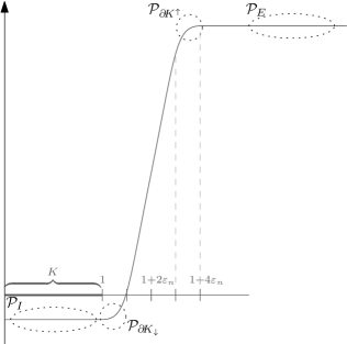
Figure 1: The Hamiltonian $H_{n}$ and the four distinguished sets of 1-periodic orbits

For what follows we fix an index $j\in{\mathbb{Z}}$ and restrict our attention to orbits of indices $j-1,j,j+1$.

Notation 5.2.

Given an index $j$ and a ${\mathbb{Z}}$-graded cochain complex $A^{*}$, we let $A^{\sim j}$ be the truncation of $A^{*}$ to degrees $j-1,j,j+1$. Note that $H^{j}(A^{*})=H^{j}(A^{\sim j})$.

It follows that in order to compute $SH^{j}(K;\Lambda)$, it is enough to consider the complexes $CF^{\sim j}(H_{n})$. Note that for $n$ large enough the actions of the orbits in $\mathcal{P}_{H}\cup{\mathcal{P}}_{\partial K^{\uparrow}}$ (having indices $j-1,j,j+1$) are strictly larger than those of the orbits in $\mathcal{P}_{\partial K_{\downarrow}}\cup\mathcal{P}_{L}$, thanks to the index boundedness; this is due to the fact that the action of a Hamiltonian orbit corresponding to a Reeb orbit is given by the $y$-intercept of the tangent to the graph of Hamiltonian in the $r$ coordinate.

We may pick acceleration data with $n$ large enough so that the action separation guarantees two essential properties:

• There are no Floer trajectories going from elements in $\mathcal{P}_{\partial K_{\uparrow}}\cup\mathcal{P}_{H}$ to elements in $\mathcal{P}_{\partial K_{\downarrow}}\cup\mathcal{P}_{L}$, since the Floer differential is action increasing; it follows that the submodule of $CF^{\sim j}(H_{n})$ generated $\mathcal{P}_{\partial K_{\uparrow}}\cup\mathcal{P}_{H}$ is in fact a subcomplex, which we denote by $CF^{\sim j}_{+}(H_{n})$. We let $CF_{-}^{\sim j}(H_{n})=CF^{\sim j}(H_{n})/CF_{+}^{\sim j}(H_{n})$ be the corresponding quotient complex, which is the free $\Lambda_{\geq 0}$-module whose basis is formed by the elements of ${\mathcal{P}}_{L}\cup{\mathcal{P}}_{K_{\downarrow}}$ of indices $j-1,j,j+1$.

• Since the homotopy from $H_{n}$ to $H_{n+1}$ is increasing, continuation trajectories increase action, therefore no continuation trajectory from $CF^{\sim j}(H_{n})$ to $CF^{\sim j}(H_{n+1})$ sends an element of $\mathcal{P}_{\partial K_{\uparrow}}\cup\mathcal{P}_{H}$ to $\mathcal{P}_{\partial K_{\downarrow}}\cup\mathcal{P}_{L}$, that is the continuation morphisms map $CF^{\sim j}_{+}(H_{n})$ into $CF^{\sim j}_{+}(H_{n+1})$.

Consider the following commutative diagram of cochain complexes and cochain maps, where the rows are short exact sequences while the middle vertical arrows are the continuation maps, while the left and right ones are induced from them:

One can verify from the definitions that taking telescope of the $1$-rays involved preserves the exactness, namely we obtain the following short exact sequence:

Note that each element in this short exact sequence is a free $\Lambda_{\geq 0}$ module, in particular the rightmost module, being free, is flat, which implies that for each $r>0$, $\operatorname{Tor}^{1}\left(\operatorname{tel}_{n}CF^{\sim j}_{-}(H_{n}),\Lambda_{[0,r)}\right)=0$, therefore using the long exact sequence associated to the Tor functors, we obtain an exact sequence:

$$0\to\operatorname*{tel}\limits_{n}CF^{\sim j}_{+}(H_{n})\otimes\Lambda_{[0,r)}\xrightarrow{\ i\ }\operatorname*{tel}\limits_{n}CF^{\sim j}(H_{n})\otimes\Lambda_{[0,r)}\xrightarrow{\ p\ }\operatorname*{tel}\limits_{n}CF_{-}^{\sim j}(H_{n})\otimes\Lambda_{[0,r)}\to 0\,.$$

Now we show that taking a projective limit over $r$ still yields a short exact sequence. Note that for all $r^{\prime}>r$, the projection $\Lambda_{[0,r^{\prime})}\to\Lambda_{[0,r)}$ is surjective, therefore by the right exactness of tensor products, so is the induced map $N\otimes\Lambda_{[0,r^{\prime})}\to N\otimes\Lambda_{[0,r)}$ for each module $N$. This is a special case of the Mittag–Leffler condition, by which $\varprojlim$ preserves exactness, thus the following sequence is exact:

$$\lx@xy@svg{\hbox{\raise 0.0pt\hbox{\kern 5.5pt\hbox{\ignorespaces\ignorespaces\ignorespaces\hbox{\vtop{\kern 0.0pt\offinterlineskip\halign{\entry@#!@&&\entry@@#!@\cr&&&&\crcr}}}\ignorespaces{\hbox{\kern-5.5pt\raise 0.0pt\hbox{\hbox{\kern 0.0pt\raise 0.0pt\hbox{\hbox{\kern 3.0pt\raise 0.0pt\hbox{$\textstyle{0\ignorespaces\ignorespaces\ignorespaces\ignorespaces}$}}}}}}}\ignorespaces\ignorespaces\ignorespaces\ignorespaces{}{\hbox{\lx@xy@droprule}}\ignorespaces{\hbox{\kern 29.5pt\raise 0.0pt\hbox{\hbox{\kern 0.0pt\raise 0.0pt\hbox{\lx@xy@tip{1}\lx@xy@tip{-1}}}}}}{\hbox{\lx@xy@droprule}}{\hbox{\lx@xy@droprule}}{\hbox{\kern 29.5pt\raise 0.0pt\hbox{\hbox{\kern 0.0pt\raise 0.0pt\hbox{\hbox{\kern 3.0pt\raise 0.0pt\hbox{$\textstyle{\widehat{\operatorname*{tel}\limits_{n}}\,CF^{\sim j}_{+}(H_{n})\ignorespaces\ignorespaces\ignorespaces\ignorespaces}$}}}}}}}\ignorespaces\ignorespaces\ignorespaces\ignorespaces{}{\hbox{\lx@xy@droprule}}\ignorespaces\ignorespaces\ignorespaces{\hbox{\kern 93.44466pt\raise 5.30833pt\hbox{{}\hbox{\kern 0.0pt\raise 0.0pt\hbox{\hbox{\kern 3.0pt\hbox{\hbox{\kern 0.0pt\raise-2.30833pt\hbox{$\scriptstyle{i}$}}}\kern 3.0pt}}}}}}\ignorespaces{\hbox{\kern 109.65045pt\raise 0.0pt\hbox{\hbox{\kern 0.0pt\raise 0.0pt\hbox{\lx@xy@tip{1}\lx@xy@tip{-1}}}}}}{\hbox{\lx@xy@droprule}}{\hbox{\lx@xy@droprule}}{\hbox{\kern 109.65045pt\raise 0.0pt\hbox{\hbox{\kern 0.0pt\raise 0.0pt\hbox{\hbox{\kern 3.0pt\raise 0.0pt\hbox{$\textstyle{\widehat{\operatorname*{tel}\limits_{n}}\,CF^{\sim j}(H_{n})\ignorespaces\ignorespaces\ignorespaces\ignorespaces}$}}}}}}}\ignorespaces\ignorespaces\ignorespaces\ignorespaces{}{\hbox{\lx@xy@droprule}}\ignorespaces\ignorespaces\ignorespaces{\hbox{\kern 173.03996pt\raise 5.1875pt\hbox{{}\hbox{\kern 0.0pt\raise 0.0pt\hbox{\hbox{\kern 3.0pt\hbox{\hbox{\kern 0.0pt\raise-0.8264pt\hbox{$\scriptstyle{p}$}}}\kern 3.0pt}}}}}}\ignorespaces{\hbox{\kern 189.8009pt\raise 0.0pt\hbox{\hbox{\kern 0.0pt\raise 0.0pt\hbox{\lx@xy@tip{1}\lx@xy@tip{-1}}}}}}{\hbox{\lx@xy@droprule}}{\hbox{\lx@xy@droprule}}{\hbox{\kern 189.8009pt\raise 0.0pt\hbox{\hbox{\kern 0.0pt\raise 0.0pt\hbox{\hbox{\kern 3.0pt\raise 0.0pt\hbox{$\textstyle{\widehat{\operatorname*{tel}\limits_{n}}\,CF_{-}^{\sim j}(H_{n})\ignorespaces\ignorespaces\ignorespaces\ignorespaces}$}}}}}}}\ignorespaces\ignorespaces\ignorespaces\ignorespaces{}{\hbox{\lx@xy@droprule}}\ignorespaces{\hbox{\kern 264.83578pt\raise 0.0pt\hbox{\hbox{\kern 0.0pt\raise 0.0pt\hbox{\lx@xy@tip{1}\lx@xy@tip{-1}}}}}}{\hbox{\lx@xy@droprule}}{\hbox{\lx@xy@droprule}}{\hbox{\kern 264.83578pt\raise 0.0pt\hbox{\hbox{\kern 0.0pt\raise 0.0pt\hbox{\hbox{\kern 3.0pt\raise 0.0pt\hbox{$\textstyle{0}$}}}}}}}\ignorespaces}}}}\ignorespaces\,. \textstyle{0\ignorespaces\ignorespaces\ignorespaces\ignorespaces} \textstyle{\widehat{\operatorname*{tel}\limits_{n}}\,CF^{\sim j}_{+}(H_{n})\ignorespaces\ignorespaces\ignorespaces\ignorespaces} \scriptstyle{i} \textstyle{\widehat{\operatorname*{tel}\limits_{n}}\,CF^{\sim j}(H_{n})\ignorespaces\ignorespaces\ignorespaces\ignorespaces} \scriptstyle{p} \textstyle{\widehat{\operatorname*{tel}\limits_{n}}\,CF_{-}^{\sim j}(H_{n})\ignorespaces\ignorespaces\ignorespaces\ignorespaces} \textstyle{0} \textstyle{0\ignorespaces\ignorespaces\ignorespaces\ignorespaces} \textstyle{\widehat{\operatorname*{tel}\limits_{n}}\,CF^{\sim j}_{+}(H_{n})\ignorespaces\ignorespaces\ignorespaces\ignorespaces} \scriptstyle{i} \textstyle{\widehat{\operatorname*{tel}\limits_{n}}\,CF^{\sim j}(H_{n})\ignorespaces\ignorespaces\ignorespaces\ignorespaces} \scriptstyle{p} \textstyle{\widehat{\operatorname*{tel}\limits_{n}}\,CF_{-}^{\sim j}(H_{n})\ignorespaces\ignorespaces\ignorespaces\ignorespaces} \textstyle{0}$$

We now analyze the homologies of each chain complex in this sequence. First, we can assume without loss of generality that the Hamiltonians $H_{n}$ are such that the continuation morphisms map $CF^{\sim j}_{+}(H_{n})$ into $T^{c}CF^{\sim j}_{+}(H_{n+1})$ for some fixed $c>0$, which implies by Lemma 5.1 that the complex $\widehat{\varinjlim}{}_{n}CF^{\sim j}(H_{n})$, is acyclic, and therefore so is the complex $\widehat{\operatorname*{tel}_{n}}\,CF^{\sim j}_{+}(H_{n})$, since the two are quasi-isomorphic. It follows that $p$ is a quasi-isomorphism.

On the other hand, the differential of $CF_{-}^{\sim j}(H_{n})$ counts Floer trajectories connecting orbits in $\mathcal{P}_{\partial K_{\downarrow}}\cup\mathcal{P}_{L}$. Since our almost complex structures are cylindrical in the “neck” region $\Sigma\!\times\!(1,1+4\varepsilon_{n})$, by the “no escape” lemma, [4, 9], all these Floer solutions are contained in $K$, and the same applies to the continuation solutions going between those generators. It follows that $\widehat{\operatorname*{tel}_{n}}\,CF_{-}^{\sim j}(H_{n})$ is quasi-isomorphic to $\widehat{SC^{\sim j}}(\widehat{K})=\widehat{\varinjlim}_{n}CF_{-}^{\sim j}(H_{n})$. It can be checked that in our case $SC^{\sim j}(\widehat{K})$ is complete, namely $SC^{\sim j}(\widehat{K})\cong\widehat{SC^{\sim j}}(\widehat{K})$. Therefore

$$SH^{j}(K;\Lambda) =H^{j}\big{(}\widehat{\operatorname{tel}}_{n}CF^{\sim j}(H_{n})\big{)}\otimes\Lambda$$

$$=H^{j}\big{(}\widehat{\operatorname{tel}}_{n}CF_{-}^{\sim j}(H_{n})\big{)}\otimes\Lambda p\text{ is a quasi-isomorphism}$$

$$=H^{j}\big{(}\widehat{\varinjlim}_{n}CF_{-}^{\sim j}(H_{n})\big{)}\otimes\Lambda$$

$$=H^{j}\big{(}\varinjlim_{n}CF_{-}^{\sim j}(H_{n})\big{)}\otimes\Lambda \varinjlim_{n}CF_{-}^{\sim j}(H_{n})\text{ is complete}$$

$$=H^{j}\big{(}\varinjlim_{n}(CF_{-}^{\sim j}(H_{n})\otimes\Lambda)\big{)}$$

$$=H^{j}\big{(}\varinjlim_{n}CF_{\operatorname{cl}}^{\sim j}(H_{n};\Lambda)\big{)}$$

$$=SH_{\operatorname{cl}}^{j}(\widehat{K};\Lambda)=SH^{j}(\widehat{K};\Lambda)\,.$$

5.3.4 The kernel of $\operatorname{res}^{M}_{K}$

Here we prove the last assertion of Theorem 1.57, that is

$$\ker\left(H^{*}(M;\Lambda)\to H^{*}(K;\Lambda)\right)\subset\ker\operatorname{res}^{M}_{K}.$$

We retain the acceleration datum $(H_{n})_{n}$ specified in the previous subsection. We compute the restriction map $\operatorname{res}^{M}_{K}\colon SC^{*}(M)\to SC^{*}(K)$ using a suitable sequence of Hamiltonians $L_{n}$ to compute ${}^{*}SC(M)$, and monotone homotopies from $L_{n}$ to $H_{n}$. The Hamiltonians $L_{n}$ are assumed to satisfy the following:

1. Fix a $C^{2}$-small everywhere negative Morse function $F$, and put $L_{n}=s_{n}F$, where $s_{n}\to 0$ a decreasing positive sequence;

2. The values of $F$ on $K$ are strictly smaller than those on $K^{c}$;

3. Along $\partial K$ the gradient of $F$ with respect to a fixed Riemannian metric is outward pointing;

4. By the $C^{2}$-smallness assumption, the only $1$-periodic orbits of $L_{n}$ are the critical points of $F$;

5. Their levels are in relation with those of $H_{n}$ as seen in Figure 2.

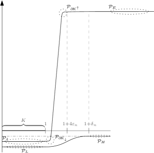
Figure 2: The Hamiltonians $L_{n}$ and $H_{n}$ with the distinguished sets of 1-periodic orbits

We denote the critical points of $L_{n}$ that lie in $K$ by $\mathcal{P}_{I}$ (for “interior”) and those that lie in $\left(K\cup\Sigma\!\times\!(1,1+\delta_{n})\right)^{c}$ by $\mathcal{P}_{E}$ (for “Exterior”). Note that the actions of the generators of $CF^{*}(L_{n})$ in $\mathcal{P}_{E}$ are greater than those of the generators of $CF^{*}(H_{n})$ in $\mathcal{P}_{\partial K_{\downarrow}}\cup\mathcal{P}_{L}$. Define $CF^{\sim j}_{+}(L_{n})$ to be the subcomplex generated by the generators in $\mathcal{P}_{E}$ and let $CF_{-}^{\sim j}(L_{n}):=CF^{\sim j}(L_{n})/CF^{\sim j}_{+}(L_{n})$ be the quotient complex. Again, by action considerations, and arguing similarly to the end of Section 5.3.3 we obtain the following homotopy-commutative diagram

$$\begin{gathered}\lx@xy@svg{\hbox{\raise 0.0pt\hbox{\kern 5.5pt\hbox{\ignorespaces\ignorespaces\ignorespaces\hbox{\vtop{\kern 0.0pt\offinterlineskip\halign{\entry@#!@&&\entry@@#!@\cr&&&&\\&&&&\crcr}}}\ignorespaces{\hbox{\kern-5.5pt\raise 0.0pt\hbox{\hbox{\kern 0.0pt\raise 0.0pt\hbox{\hbox{\kern 3.0pt\raise 0.0pt\hbox{$\textstyle{0\ignorespaces\ignorespaces\ignorespaces\ignorespaces}$}}}}}}}\ignorespaces\ignorespaces\ignorespaces\ignorespaces{}{\hbox{\lx@xy@droprule}}\ignorespaces{\hbox{\kern 30.6597pt\raise 0.0pt\hbox{\hbox{\kern 0.0pt\raise 0.0pt\hbox{\lx@xy@tip{1}\lx@xy@tip{-1}}}}}}{\hbox{\lx@xy@droprule}}{\hbox{\lx@xy@droprule}}{\hbox{\kern 30.6597pt\raise 0.0pt\hbox{\hbox{\kern 0.0pt\raise 0.0pt\hbox{\hbox{\kern 3.0pt\raise 0.0pt\hbox{$\textstyle{\widehat{\operatorname*{tel}\limits_{n}}\,CF^{\sim j}_{+}(L_{n})\ignorespaces\ignorespaces\ignorespaces\ignorespaces\ignorespaces\ignorespaces\ignorespaces\ignorespaces}$}}}}}}}\ignorespaces\ignorespaces\ignorespaces\ignorespaces{}{\hbox{\lx@xy@droprule}}\ignorespaces{\hbox{\kern 57.57523pt\raise-29.49998pt\hbox{\hbox{\kern 0.0pt\raise 0.0pt\hbox{\lx@xy@tip{1}\lx@xy@tip{-1}}}}}}{\hbox{\lx@xy@droprule}}{\hbox{\lx@xy@droprule}}\ignorespaces\ignorespaces\ignorespaces\ignorespaces{}{\hbox{\lx@xy@droprule}}\ignorespaces\ignorespaces\ignorespaces{\hbox{\kern 93.44466pt\raise 5.30833pt\hbox{{}\hbox{\kern 0.0pt\raise 0.0pt\hbox{\hbox{\kern 3.0pt\hbox{\hbox{\kern 0.0pt\raise-2.30833pt\hbox{$\scriptstyle{i}$}}}\kern 3.0pt}}}}}}\ignorespaces{\hbox{\kern 110.81015pt\raise 0.0pt\hbox{\hbox{\kern 0.0pt\raise 0.0pt\hbox{\lx@xy@tip{1}\lx@xy@tip{-1}}}}}}{\hbox{\lx@xy@droprule}}{\hbox{\lx@xy@droprule}}{\hbox{\kern 110.81015pt\raise 0.0pt\hbox{\hbox{\kern 0.0pt\raise 0.0pt\hbox{\hbox{\kern 3.0pt\raise 0.0pt\hbox{$\textstyle{\widehat{\operatorname*{tel}\limits_{n}}\,CF^{\sim j}(L_{n})\ignorespaces\ignorespaces\ignorespaces\ignorespaces\ignorespaces\ignorespaces\ignorespaces\ignorespaces}$}}}}}}}\ignorespaces\ignorespaces\ignorespaces\ignorespaces{}{\hbox{\lx@xy@droprule}}\ignorespaces{\hbox{\kern 137.72568pt\raise-29.49998pt\hbox{\hbox{\kern 0.0pt\raise 0.0pt\hbox{\lx@xy@tip{1}\lx@xy@tip{-1}}}}}}{\hbox{\lx@xy@droprule}}{\hbox{\lx@xy@droprule}}\ignorespaces\ignorespaces\ignorespaces\ignorespaces{}{\hbox{\lx@xy@droprule}}\ignorespaces\ignorespaces\ignorespaces{\hbox{\kern 173.03996pt\raise 5.1875pt\hbox{{}\hbox{\kern 0.0pt\raise 0.0pt\hbox{\hbox{\kern 3.0pt\hbox{\hbox{\kern 0.0pt\raise-0.8264pt\hbox{$\scriptstyle{p}$}}}\kern 3.0pt}}}}}}\ignorespaces{\hbox{\kern 190.9606pt\raise 0.0pt\hbox{\hbox{\kern 0.0pt\raise 0.0pt\hbox{\lx@xy@tip{1}\lx@xy@tip{-1}}}}}}{\hbox{\lx@xy@droprule}}{\hbox{\lx@xy@droprule}}{\hbox{\kern 190.9606pt\raise 0.0pt\hbox{\hbox{\kern 0.0pt\raise 0.0pt\hbox{\hbox{\kern 3.0pt\raise 0.0pt\hbox{$\textstyle{\widehat{\operatorname*{tel}\limits_{n}}\,CF_{-}^{\sim j}(L_{n})\ignorespaces\ignorespaces\ignorespaces\ignorespaces\ignorespaces\ignorespaces\ignorespaces\ignorespaces}$}}}}}}}\ignorespaces\ignorespaces\ignorespaces\ignorespaces{}{\hbox{\lx@xy@droprule}}\ignorespaces{\hbox{\kern 215.31834pt\raise-29.49998pt\hbox{\hbox{\kern 0.0pt\raise 0.0pt\hbox{\lx@xy@tip{1}\lx@xy@tip{-1}}}}}}{\hbox{\lx@xy@droprule}}{\hbox{\lx@xy@droprule}}\ignorespaces\ignorespaces\ignorespaces\ignorespaces{}{\hbox{\lx@xy@droprule}}\ignorespaces{\hbox{\kern 264.83578pt\raise 0.0pt\hbox{\hbox{\kern 0.0pt\raise 0.0pt\hbox{\lx@xy@tip{1}\lx@xy@tip{-1}}}}}}{\hbox{\lx@xy@droprule}}{\hbox{\lx@xy@droprule}}{\hbox{\kern 264.83578pt\raise 0.0pt\hbox{\hbox{\kern 0.0pt\raise 0.0pt\hbox{\hbox{\kern 3.0pt\raise 0.0pt\hbox{$\textstyle{0}$}}}}}}}{\hbox{\kern-5.5pt\raise-41.17996pt\hbox{\hbox{\kern 0.0pt\raise 0.0pt\hbox{\hbox{\kern 3.0pt\raise 0.0pt\hbox{$\textstyle{0\ignorespaces\ignorespaces\ignorespaces\ignorespaces}$}}}}}}}\ignorespaces\ignorespaces\ignorespaces\ignorespaces{}{\hbox{\lx@xy@droprule}}\ignorespaces{\hbox{\kern 29.5pt\raise-41.17996pt\hbox{\hbox{\kern 0.0pt\raise 0.0pt\hbox{\lx@xy@tip{1}\lx@xy@tip{-1}}}}}}{\hbox{\lx@xy@droprule}}{\hbox{\lx@xy@droprule}}{\hbox{\kern 29.5pt\raise-41.17996pt\hbox{\hbox{\kern 0.0pt\raise 0.0pt\hbox{\hbox{\kern 3.0pt\raise 0.0pt\hbox{$\textstyle{\widehat{\operatorname*{tel}\limits_{n}}\,CF^{\sim j}_{+}(H_{n})\ignorespaces\ignorespaces\ignorespaces\ignorespaces}$}}}}}}}\ignorespaces\ignorespaces\ignorespaces\ignorespaces{}{\hbox{\lx@xy@droprule}}\ignorespaces\ignorespaces\ignorespaces{\hbox{\kern 93.44466pt\raise-35.87163pt\hbox{{}\hbox{\kern 0.0pt\raise 0.0pt\hbox{\hbox{\kern 3.0pt\hbox{\hbox{\kern 0.0pt\raise-2.30833pt\hbox{$\scriptstyle{i}$}}}\kern 3.0pt}}}}}}\ignorespaces{\hbox{\kern 109.65045pt\raise-41.17996pt\hbox{\hbox{\kern 0.0pt\raise 0.0pt\hbox{\lx@xy@tip{1}\lx@xy@tip{-1}}}}}}{\hbox{\lx@xy@droprule}}{\hbox{\lx@xy@droprule}}{\hbox{\kern 109.65045pt\raise-41.17996pt\hbox{\hbox{\kern 0.0pt\raise 0.0pt\hbox{\hbox{\kern 3.0pt\raise 0.0pt\hbox{$\textstyle{\widehat{\operatorname*{tel}\limits_{n}}\,CF^{\sim j}(H_{n})\ignorespaces\ignorespaces\ignorespaces\ignorespaces}$}}}}}}}\ignorespaces\ignorespaces\ignorespaces\ignorespaces{}{\hbox{\lx@xy@droprule}}\ignorespaces\ignorespaces\ignorespaces{\hbox{\kern 173.03996pt\raise-35.99246pt\hbox{{}\hbox{\kern 0.0pt\raise 0.0pt\hbox{\hbox{\kern 3.0pt\hbox{\hbox{\kern 0.0pt\raise-0.8264pt\hbox{$\scriptstyle{p}$}}}\kern 3.0pt}}}}}}\ignorespaces{\hbox{\kern 189.8009pt\raise-41.17996pt\hbox{\hbox{\kern 0.0pt\raise 0.0pt\hbox{\lx@xy@tip{1}\lx@xy@tip{-1}}}}}}{\hbox{\lx@xy@droprule}}{\hbox{\lx@xy@droprule}}{\hbox{\kern 189.8009pt\raise-41.17996pt\hbox{\hbox{\kern 0.0pt\raise 0.0pt\hbox{\hbox{\kern 3.0pt\raise 0.0pt\hbox{$\textstyle{\widehat{\operatorname*{tel}\limits_{n}}\,CF_{-}^{\sim j}(H_{n})\ignorespaces\ignorespaces\ignorespaces\ignorespaces}$}}}}}}}\ignorespaces\ignorespaces\ignorespaces\ignorespaces{}{\hbox{\lx@xy@droprule}}\ignorespaces{\hbox{\kern 264.83578pt\raise-41.17996pt\hbox{\hbox{\kern 0.0pt\raise 0.0pt\hbox{\lx@xy@tip{1}\lx@xy@tip{-1}}}}}}{\hbox{\lx@xy@droprule}}{\hbox{\lx@xy@droprule}}{\hbox{\kern 264.83578pt\raise-41.17996pt\hbox{\hbox{\kern 0.0pt\raise 0.0pt\hbox{\hbox{\kern 3.0pt\raise 0.0pt\hbox{$\textstyle{0}$}}}}}}}\ignorespaces}}}}\ignorespaces\end{gathered} \textstyle{0\ignorespaces\ignorespaces\ignorespaces\ignorespaces} \textstyle{\widehat{\operatorname*{tel}\limits_{n}}\,CF^{\sim j}_{+}(L_{n})\ignorespaces\ignorespaces\ignorespaces\ignorespaces\ignorespaces\ignorespaces\ignorespaces\ignorespaces} \scriptstyle{i} \textstyle{\widehat{\operatorname*{tel}\limits_{n}}\,CF^{\sim j}(L_{n})\ignorespaces\ignorespaces\ignorespaces\ignorespaces\ignorespaces\ignorespaces\ignorespaces\ignorespaces} \scriptstyle{p} \textstyle{\widehat{\operatorname*{tel}\limits_{n}}\,CF_{-}^{\sim j}(L_{n})\ignorespaces\ignorespaces\ignorespaces\ignorespaces\ignorespaces\ignorespaces\ignorespaces\ignorespaces} \textstyle{0} \textstyle{0\ignorespaces\ignorespaces\ignorespaces\ignorespaces} \textstyle{\widehat{\operatorname*{tel}\limits_{n}}\,CF^{\sim j}_{+}(H_{n})\ignorespaces\ignorespaces\ignorespaces\ignorespaces} \scriptstyle{i} \textstyle{\widehat{\operatorname*{tel}\limits_{n}}\,CF^{\sim j}(H_{n})\ignorespaces\ignorespaces\ignorespaces\ignorespaces} \scriptstyle{p} \textstyle{\widehat{\operatorname*{tel}\limits_{n}}\,CF_{-}^{\sim j}(H_{n})\ignorespaces\ignorespaces\ignorespaces\ignorespaces} \textstyle{0} \textstyle{0\ignorespaces\ignorespaces\ignorespaces\ignorespaces} \textstyle{\widehat{\operatorname*{tel}\limits_{n}}\,CF^{\sim j}_{+}(L_{n})\ignorespaces\ignorespaces\ignorespaces\ignorespaces\ignorespaces\ignorespaces\ignorespaces\ignorespaces} \scriptstyle{i} \textstyle{\widehat{\operatorname*{tel}\limits_{n}}\,CF^{\sim j}(L_{n})\ignorespaces\ignorespaces\ignorespaces\ignorespaces\ignorespaces\ignorespaces\ignorespaces\ignorespaces} \scriptstyle{p} \textstyle{\widehat{\operatorname*{tel}\limits_{n}}\,CF_{-}^{\sim j}(L_{n})\ignorespaces\ignorespaces\ignorespaces\ignorespaces\ignorespaces\ignorespaces\ignorespaces\ignorespaces} \textstyle{0} \textstyle{0\ignorespaces\ignorespaces\ignorespaces\ignorespaces} \textstyle{\widehat{\operatorname*{tel}\limits_{n}}\,CF^{\sim j}_{+}(H_{n})\ignorespaces\ignorespaces\ignorespaces\ignorespaces} \scriptstyle{i} \textstyle{\widehat{\operatorname*{tel}\limits_{n}}\,CF^{\sim j}(H_{n})\ignorespaces\ignorespaces\ignorespaces\ignorespaces} \scriptstyle{p} \textstyle{\widehat{\operatorname*{tel}\limits_{n}}\,CF_{-}^{\sim j}(H_{n})\ignorespaces\ignorespaces\ignorespaces\ignorespaces} \textstyle{0}$$ (20)

Let us identify the relevant complexes. By a calculation as in [27], $\widehat{\operatorname*{tel}_{n}}\,CF^{\sim j}(L_{n})$ computes $SH^{j}(M)=H^{j}(M)\otimes\Lambda_{>0}$. The complex $\widehat{\operatorname*{tel}\limits_{n}}\,CF_{-}^{\sim j}(L_{n})$ is quasi-isomorphic to $\widehat{\varinjlim_{n}}CF_{-}^{\sim j}(L_{n})=\Lambda_{>0}\otimes\{x\in{\mathcal{P}}_{I}\,|\,x\text{ has index }j-1,j,j+1\}$, where the differential counts Morse flow lines of $F$ between the critical points of $F$ in ${\mathcal{P}}_{I}$. It follows that this complex computes $H^{j}(K)\otimes\Lambda_{>0}$. Similarly to the considerations of Section 5.3.3, the complex $\widehat{\operatorname{tel}}_{n}\,CF^{\sim j}_{+}(H_{n})$ is acyclic. Therefore, taking the homology of the right square of (20) we obtain the commutative diagram

where $i^{*}$ is the restriction on singular cohomology. It follows from this diagram that $\ker i^{*}\subset\ker\operatorname{res}^{M}_{K}$. This completes the proof of Theorem 1.57.

5.4 Proof of Theorem 2.4

Here we prove Theorem 2.4, which asserts the existence of an exact triangle relating $SH^{*}(M,K;\Lambda)$, $H^{*}(M,K;\Lambda)$, and $SH^{+}(\widehat{K};\Lambda)$, which is an invariant defined, for instance in [4]. The complex computing this invariant is obtained by quotienting $SC^{*}(\widehat{K})$ by the subcomplex generated by the critical points of the Morse functions $(H^{\mu_{n}}|_{K})_{n}$, see Section 5.3.2.

We repeat the arguments of the previous section, only this time we impose an extra condition on $L_{n}$ and $H_{n}$: they are chosen so that they coincide in $K$. Picking up from the commutative diagram (20), labeling arrows relevant to us and identifying the chain complexes with known ones, we arrive at:

$$\begin{gathered}\lx@xy@svg{\hbox{\raise 0.0pt\hbox{\kern 5.5pt\hbox{\ignorespaces\ignorespaces\ignorespaces\hbox{\vtop{\kern 0.0pt\offinterlineskip\halign{\entry@#!@&&\entry@@#!@\cr&&&&\\&&&&\crcr}}}\ignorespaces{\hbox{\kern-5.5pt\raise 0.0pt\hbox{\hbox{\kern 0.0pt\raise 0.0pt\hbox{\hbox{\kern 3.0pt\raise 0.0pt\hbox{$\textstyle{0\ignorespaces\ignorespaces\ignorespaces\ignorespaces}$}}}}}}}\ignorespaces\ignorespaces\ignorespaces\ignorespaces{}{\hbox{\lx@xy@droprule}}\ignorespaces{\hbox{\kern 29.5pt\raise 0.0pt\hbox{\hbox{\kern 0.0pt\raise 0.0pt\hbox{\lx@xy@tip{1}\lx@xy@tip{-1}}}}}}{\hbox{\lx@xy@droprule}}{\hbox{\lx@xy@droprule}}{\hbox{\kern 29.5pt\raise 0.0pt\hbox{\hbox{\kern 0.0pt\raise 0.0pt\hbox{\hbox{\kern 3.0pt\raise 0.0pt\hbox{$\textstyle{C^{\sim j}(M,K)\otimes\Lambda_{>0}\ignorespaces\ignorespaces\ignorespaces\ignorespaces\ignorespaces\ignorespaces\ignorespaces\ignorespaces}$}}}}}}}\ignorespaces\ignorespaces\ignorespaces\ignorespaces{}{\hbox{\lx@xy@droprule}}\ignorespaces\ignorespaces\ignorespaces{\hbox{\kern 68.91675pt\raise-20.58998pt\hbox{{}\hbox{\kern 0.0pt\raise 0.0pt\hbox{\hbox{\kern 3.0pt\hbox{\hbox{\kern 0.0pt\raise-1.64168pt\hbox{$\scriptstyle{\Phi_{+}}$}}}\kern 3.0pt}}}}}}\ignorespaces{\hbox{\kern 68.91675pt\raise-29.49998pt\hbox{\hbox{\kern 0.0pt\raise 0.0pt\hbox{\lx@xy@tip{1}\lx@xy@tip{-1}}}}}}{\hbox{\lx@xy@droprule}}{\hbox{\lx@xy@droprule}}\ignorespaces\ignorespaces\ignorespaces\ignorespaces{}{\hbox{\lx@xy@droprule}}\ignorespaces\ignorespaces\ignorespaces{\hbox{\kern 116.1277pt\raise 5.30833pt\hbox{{}\hbox{\kern 0.0pt\raise 0.0pt\hbox{\hbox{\kern 3.0pt\hbox{\hbox{\kern 0.0pt\raise-2.30833pt\hbox{$\scriptstyle{i}$}}}\kern 3.0pt}}}}}}\ignorespaces{\hbox{\kern 132.3335pt\raise 0.0pt\hbox{\hbox{\kern 0.0pt\raise 0.0pt\hbox{\lx@xy@tip{1}\lx@xy@tip{-1}}}}}}{\hbox{\lx@xy@droprule}}{\hbox{\lx@xy@droprule}}{\hbox{\kern 132.3335pt\raise 0.0pt\hbox{\hbox{\kern 0.0pt\raise 0.0pt\hbox{\hbox{\kern 3.0pt\raise 0.0pt\hbox{$\textstyle{C^{\sim j}(M)\otimes\Lambda_{>0}\ignorespaces\ignorespaces\ignorespaces\ignorespaces\ignorespaces\ignorespaces\ignorespaces\ignorespaces}$}}}}}}}\ignorespaces\ignorespaces\ignorespaces\ignorespaces{}{\hbox{\lx@xy@droprule}}\ignorespaces\ignorespaces\ignorespaces{\hbox{\kern 165.20166pt\raise-20.58998pt\hbox{{}\hbox{\kern 0.0pt\raise 0.0pt\hbox{\hbox{\kern 3.0pt\hbox{\hbox{\kern 0.0pt\raise-2.39166pt\hbox{$\scriptstyle{\Phi}$}}}\kern 3.0pt}}}}}}\ignorespaces{\hbox{\kern 165.20166pt\raise-29.49998pt\hbox{\hbox{\kern 0.0pt\raise 0.0pt\hbox{\lx@xy@tip{1}\lx@xy@tip{-1}}}}}}{\hbox{\lx@xy@droprule}}{\hbox{\lx@xy@droprule}}\ignorespaces\ignorespaces\ignorespaces\ignorespaces{}{\hbox{\lx@xy@droprule}}\ignorespaces\ignorespaces\ignorespaces{\hbox{\kern 203.94777pt\raise 5.87083pt\hbox{{}\hbox{\kern 0.0pt\raise 0.0pt\hbox{\hbox{\kern 3.0pt\hbox{\hbox{\kern 0.0pt\raise-1.50974pt\hbox{$\scriptstyle{p^{L}}$}}}\kern 3.0pt}}}}}}\ignorespaces{\hbox{\kern 222.06982pt\raise 0.0pt\hbox{\hbox{\kern 0.0pt\raise 0.0pt\hbox{\lx@xy@tip{1}\lx@xy@tip{-1}}}}}}{\hbox{\lx@xy@droprule}}{\hbox{\lx@xy@droprule}}{\hbox{\kern 222.06982pt\raise 0.0pt\hbox{\hbox{\kern 0.0pt\raise 0.0pt\hbox{\hbox{\kern 3.0pt\raise 0.0pt\hbox{$\textstyle{C^{\sim j}(K)\otimes\Lambda_{>0}\ignorespaces\ignorespaces\ignorespaces\ignorespaces\ignorespaces\ignorespaces\ignorespaces\ignorespaces}$}}}}}}}\ignorespaces\ignorespaces\ignorespaces\ignorespaces{}{\hbox{\lx@xy@droprule}}\ignorespaces\ignorespaces\ignorespaces{\hbox{\kern 254.14632pt\raise-20.58998pt\hbox{{}\hbox{\kern 0.0pt\raise 0.0pt\hbox{\hbox{\kern 3.0pt\hbox{\hbox{\kern 0.0pt\raise-1.31944pt\hbox{$\scriptstyle{\Phi_{Q}}$}}}\kern 3.0pt}}}}}}\ignorespaces{\hbox{\kern 254.14632pt\raise-29.49998pt\hbox{\hbox{\kern 0.0pt\raise 0.0pt\hbox{\lx@xy@tip{1}\lx@xy@tip{-1}}}}}}{\hbox{\lx@xy@droprule}}{\hbox{\lx@xy@droprule}}\ignorespaces\ignorespaces\ignorespaces\ignorespaces{}{\hbox{\lx@xy@droprule}}\ignorespaces{\hbox{\kern 312.44502pt\raise 0.0pt\hbox{\hbox{\kern 0.0pt\raise 0.0pt\hbox{\lx@xy@tip{1}\lx@xy@tip{-1}}}}}}{\hbox{\lx@xy@droprule}}{\hbox{\lx@xy@droprule}}{\hbox{\kern 312.44502pt\raise 0.0pt\hbox{\hbox{\kern 0.0pt\raise 0.0pt\hbox{\hbox{\kern 3.0pt\raise 0.0pt\hbox{$\textstyle{0}$}}}}}}}{\hbox{\kern-5.5pt\raise-41.17996pt\hbox{\hbox{\kern 0.0pt\raise 0.0pt\hbox{\hbox{\kern 3.0pt\raise 0.0pt\hbox{$\textstyle{0\ignorespaces\ignorespaces\ignorespaces\ignorespaces}$}}}}}}}\ignorespaces\ignorespaces\ignorespaces\ignorespaces{}{\hbox{\lx@xy@droprule}}\ignorespaces{\hbox{\kern 40.84152pt\raise-41.17996pt\hbox{\hbox{\kern 0.0pt\raise 0.0pt\hbox{\lx@xy@tip{1}\lx@xy@tip{-1}}}}}}{\hbox{\lx@xy@droprule}}{\hbox{\lx@xy@droprule}}{\hbox{\kern 40.84152pt\raise-41.17996pt\hbox{\hbox{\kern 0.0pt\raise 0.0pt\hbox{\hbox{\kern 3.0pt\raise 0.0pt\hbox{$\textstyle{\widehat{\operatorname*{tel}\limits_{n}}\,CF^{\sim j}_{+}(H_{n})\ignorespaces\ignorespaces\ignorespaces\ignorespaces}$}}}}}}}\ignorespaces\ignorespaces\ignorespaces\ignorespaces{}{\hbox{\lx@xy@droprule}}\ignorespaces\ignorespaces\ignorespaces{\hbox{\kern 115.75624pt\raise-35.87163pt\hbox{{}\hbox{\kern 0.0pt\raise 0.0pt\hbox{\hbox{\kern 3.0pt\hbox{\hbox{\kern 0.0pt\raise-2.30833pt\hbox{$\scriptstyle{i}$}}}\kern 3.0pt}}}}}}\ignorespaces{\hbox{\kern 142.93208pt\raise-41.17996pt\hbox{\hbox{\kern 0.0pt\raise 0.0pt\hbox{\lx@xy@tip{1}\lx@xy@tip{-1}}}}}}{\hbox{\lx@xy@droprule}}{\hbox{\lx@xy@droprule}}{\hbox{\kern 142.93208pt\raise-41.17996pt\hbox{\hbox{\kern 0.0pt\raise 0.0pt\hbox{\hbox{\kern 3.0pt\raise 0.0pt\hbox{$\textstyle{SC^{\sim j}(K)\ignorespaces\ignorespaces\ignorespaces\ignorespaces}$}}}}}}}\ignorespaces\ignorespaces\ignorespaces\ignorespaces{}{\hbox{\lx@xy@droprule}}\ignorespaces\ignorespaces\ignorespaces{\hbox{\kern 203.38718pt\raise-47.19801pt\hbox{{}\hbox{\kern 0.0pt\raise 0.0pt\hbox{\hbox{\kern 3.0pt\hbox{\hbox{\kern 0.0pt\raise-1.65695pt\hbox{$\scriptstyle{\text{qis}}$}}}\kern 3.0pt}}}}}}\ignorespaces\ignorespaces\ignorespaces{\hbox{\kern 204.00124pt\raise-35.30913pt\hbox{{}\hbox{\kern 0.0pt\raise 0.0pt\hbox{\hbox{\kern 3.0pt\hbox{\hbox{\kern 0.0pt\raise-1.50974pt\hbox{$\scriptstyle{p^{H}}$}}}\kern 3.0pt}}}}}}\ignorespaces{\hbox{\kern 233.70311pt\raise-41.17996pt\hbox{\hbox{\kern 0.0pt\raise 0.0pt\hbox{\lx@xy@tip{1}\lx@xy@tip{-1}}}}}}{\hbox{\lx@xy@droprule}}{\hbox{\lx@xy@droprule}}{\hbox{\kern 233.70311pt\raise-41.17996pt\hbox{\hbox{\kern 0.0pt\raise 0.0pt\hbox{\hbox{\kern 3.0pt\raise 0.0pt\hbox{$\textstyle{SC^{\sim j}(\widehat{K})\ignorespaces\ignorespaces\ignorespaces\ignorespaces}$}}}}}}}\ignorespaces\ignorespaces\ignorespaces\ignorespaces{}{\hbox{\lx@xy@droprule}}\ignorespaces{\hbox{\kern 310.22281pt\raise-41.17996pt\hbox{\hbox{\kern 0.0pt\raise 0.0pt\hbox{\lx@xy@tip{1}\lx@xy@tip{-1}}}}}}{\hbox{\lx@xy@droprule}}{\hbox{\lx@xy@droprule}}{\hbox{\kern 310.22281pt\raise-41.17996pt\hbox{\hbox{\kern 0.0pt\raise 0.0pt\hbox{\hbox{\kern 3.0pt\raise 0.0pt\hbox{$\textstyle{0\,.}$}}}}}}}\ignorespaces}}}}\ignorespaces\end{gathered} \textstyle{0\ignorespaces\ignorespaces\ignorespaces\ignorespaces} \textstyle{C^{\sim j}(M,K)\otimes\Lambda_{>0}\ignorespaces\ignorespaces\ignorespaces\ignorespaces\ignorespaces\ignorespaces\ignorespaces\ignorespaces} \scriptstyle{\Phi_{+}} \scriptstyle{i} \textstyle{C^{\sim j}(M)\otimes\Lambda_{>0}\ignorespaces\ignorespaces\ignorespaces\ignorespaces\ignorespaces\ignorespaces\ignorespaces\ignorespaces} \scriptstyle{\Phi} \scriptstyle{p^{L}} \textstyle{C^{\sim j}(K)\otimes\Lambda_{>0}\ignorespaces\ignorespaces\ignorespaces\ignorespaces\ignorespaces\ignorespaces\ignorespaces\ignorespaces} \scriptstyle{\Phi_{Q}} \textstyle{0} \textstyle{0\ignorespaces\ignorespaces\ignorespaces\ignorespaces} \textstyle{\widehat{\operatorname*{tel}\limits_{n}}\,CF^{\sim j}_{+}(H_{n})\ignorespaces\ignorespaces\ignorespaces\ignorespaces} \scriptstyle{i} \textstyle{SC^{\sim j}(K)\ignorespaces\ignorespaces\ignorespaces\ignorespaces} \scriptstyle{p^{H}} \textstyle{SC^{\sim j}(\widehat{K})\ignorespaces\ignorespaces\ignorespaces\ignorespaces} \textstyle{0\,.} \textstyle{0\ignorespaces\ignorespaces\ignorespaces\ignorespaces} \textstyle{C^{\sim j}(M,K)\otimes\Lambda_{>0}\ignorespaces\ignorespaces\ignorespaces\ignorespaces\ignorespaces\ignorespaces\ignorespaces\ignorespaces} \scriptstyle{\Phi_{+}} \scriptstyle{i} \textstyle{C^{\sim j}(M)\otimes\Lambda_{>0}\ignorespaces\ignorespaces\ignorespaces\ignorespaces\ignorespaces\ignorespaces\ignorespaces\ignorespaces} \scriptstyle{\Phi} \scriptstyle{p^{L}} \textstyle{C^{\sim j}(K)\otimes\Lambda_{>0}\ignorespaces\ignorespaces\ignorespaces\ignorespaces\ignorespaces\ignorespaces\ignorespaces\ignorespaces} \scriptstyle{\Phi_{Q}} \textstyle{0} \textstyle{0\ignorespaces\ignorespaces\ignorespaces\ignorespaces} \textstyle{\widehat{\operatorname*{tel}\limits_{n}}\,CF^{\sim j}_{+}(H_{n})\ignorespaces\ignorespaces\ignorespaces\ignorespaces} \scriptstyle{i} \textstyle{SC^{\sim j}(K)\ignorespaces\ignorespaces\ignorespaces\ignorespaces} \scriptstyle{p^{H}} \textstyle{SC^{\sim j}(\widehat{K})\ignorespaces\ignorespaces\ignorespaces\ignorespaces} \textstyle{0\,.}$$

Note that $p^{H}$ is a quasi-isomorphism. Passing to cones of the vertical morphisms, we obtain the following $3$x$3$ square of exact sequences (both horizontal and vertical)

$$\begin{gathered}\lx@xy@svg{\hbox{\raise 0.0pt\hbox{\kern 5.5pt\hbox{\ignorespaces\ignorespaces\ignorespaces\hbox{\vtop{\kern 0.0pt\offinterlineskip\halign{\entry@#!@&&\entry@@#!@\cr&&&&\\&&&&\\&&&&\\&&&&\\&&&\crcr}}}\ignorespaces{\hbox{\kern-3.0pt\raise 0.0pt\hbox{\hbox{\kern 0.0pt\raise 0.0pt\hbox{\hbox{\kern 3.0pt\raise 0.0pt\hbox{$\textstyle{}$}}}}}}}{\hbox{\kern 55.53348pt\raise 0.0pt\hbox{\hbox{\kern 0.0pt\raise 0.0pt\hbox{\hbox{\kern 3.0pt\raise 0.0pt\hbox{$\textstyle{0\ignorespaces\ignorespaces\ignorespaces\ignorespaces}$}}}}}}}\ignorespaces\ignorespaces\ignorespaces\ignorespaces{}{\hbox{\lx@xy@droprule}}\ignorespaces{\hbox{\kern 61.03348pt\raise-27.13222pt\hbox{\hbox{\kern 0.0pt\raise 0.0pt\hbox{\lx@xy@tip{1}\lx@xy@tip{-1}}}}}}{\hbox{\lx@xy@droprule}}{\hbox{\lx@xy@droprule}}{\hbox{\kern 136.05183pt\raise 0.0pt\hbox{\hbox{\kern 0.0pt\raise 0.0pt\hbox{\hbox{\kern 3.0pt\raise 0.0pt\hbox{$\textstyle{0\ignorespaces\ignorespaces\ignorespaces\ignorespaces}$}}}}}}}\ignorespaces\ignorespaces\ignorespaces\ignorespaces{}{\hbox{\lx@xy@droprule}}\ignorespaces{\hbox{\kern 141.55183pt\raise-27.13222pt\hbox{\hbox{\kern 0.0pt\raise 0.0pt\hbox{\lx@xy@tip{1}\lx@xy@tip{-1}}}}}}{\hbox{\lx@xy@droprule}}{\hbox{\lx@xy@droprule}}{\hbox{\kern 209.22993pt\raise 0.0pt\hbox{\hbox{\kern 0.0pt\raise 0.0pt\hbox{\hbox{\kern 3.0pt\raise 0.0pt\hbox{$\textstyle{0\ignorespaces\ignorespaces\ignorespaces\ignorespaces}$}}}}}}}\ignorespaces\ignorespaces\ignorespaces\ignorespaces{}{\hbox{\lx@xy@droprule}}\ignorespaces{\hbox{\kern 214.72993pt\raise-27.13222pt\hbox{\hbox{\kern 0.0pt\raise 0.0pt\hbox{\lx@xy@tip{1}\lx@xy@tip{-1}}}}}}{\hbox{\lx@xy@droprule}}{\hbox{\lx@xy@droprule}}{\hbox{\kern 265.42316pt\raise 0.0pt\hbox{\hbox{\kern 0.0pt\raise 0.0pt\hbox{\hbox{\kern 3.0pt\raise 0.0pt\hbox{$\textstyle{}$}}}}}}}{\hbox{\kern-5.5pt\raise-38.8122pt\hbox{\hbox{\kern 0.0pt\raise 0.0pt\hbox{\hbox{\kern 3.0pt\raise 0.0pt\hbox{$\textstyle{0\ignorespaces\ignorespaces\ignorespaces\ignorespaces}$}}}}}}}\ignorespaces\ignorespaces\ignorespaces\ignorespaces{}{\hbox{\lx@xy@droprule}}\ignorespaces{\hbox{\kern 32.95825pt\raise-38.8122pt\hbox{\hbox{\kern 0.0pt\raise 0.0pt\hbox{\lx@xy@tip{1}\lx@xy@tip{-1}}}}}}{\hbox{\lx@xy@droprule}}{\hbox{\lx@xy@droprule}}{\hbox{\kern 32.95825pt\raise-38.8122pt\hbox{\hbox{\kern 0.0pt\raise 0.0pt\hbox{\hbox{\kern 3.0pt\raise 0.0pt\hbox{$\textstyle{\widehat{\operatorname*{tel}\limits_{n}}\,CF^{\sim j}_{+}(H_{n})\ignorespaces\ignorespaces\ignorespaces\ignorespaces\ignorespaces\ignorespaces\ignorespaces\ignorespaces}$}}}}}}}\ignorespaces\ignorespaces\ignorespaces\ignorespaces{}{\hbox{\lx@xy@droprule}}\ignorespaces{\hbox{\kern 61.03348pt\raise-69.15327pt\hbox{\hbox{\kern 0.0pt\raise 0.0pt\hbox{\lx@xy@tip{1}\lx@xy@tip{-1}}}}}}{\hbox{\lx@xy@droprule}}{\hbox{\lx@xy@droprule}}\ignorespaces\ignorespaces\ignorespaces\ignorespaces{}{\hbox{\lx@xy@droprule}}\ignorespaces\ignorespaces\ignorespaces{\hbox{\kern 100.22441pt\raise-33.50386pt\hbox{{}\hbox{\kern 0.0pt\raise 0.0pt\hbox{\hbox{\kern 3.0pt\hbox{\hbox{\kern 0.0pt\raise-2.30833pt\hbox{$\scriptstyle{i}$}}}\kern 3.0pt}}}}}}\ignorespaces{\hbox{\kern 119.75171pt\raise-38.8122pt\hbox{\hbox{\kern 0.0pt\raise 0.0pt\hbox{\lx@xy@tip{1}\lx@xy@tip{-1}}}}}}{\hbox{\lx@xy@droprule}}{\hbox{\lx@xy@droprule}}{\hbox{\kern 119.75171pt\raise-38.8122pt\hbox{\hbox{\kern 0.0pt\raise 0.0pt\hbox{\hbox{\kern 3.0pt\raise 0.0pt\hbox{$\textstyle{SC_{M}^{\sim j}(K)\ignorespaces\ignorespaces\ignorespaces\ignorespaces\ignorespaces\ignorespaces\ignorespaces\ignorespaces}$}}}}}}}\ignorespaces\ignorespaces\ignorespaces\ignorespaces{}{\hbox{\lx@xy@droprule}}\ignorespaces{\hbox{\kern 141.55183pt\raise-69.15327pt\hbox{\hbox{\kern 0.0pt\raise 0.0pt\hbox{\lx@xy@tip{1}\lx@xy@tip{-1}}}}}}{\hbox{\lx@xy@droprule}}{\hbox{\lx@xy@droprule}}\ignorespaces\ignorespaces\ignorespaces\ignorespaces{}{\hbox{\lx@xy@droprule}}\ignorespaces\ignorespaces\ignorespaces{\hbox{\kern 171.61934pt\raise-44.83025pt\hbox{{}\hbox{\kern 0.0pt\raise 0.0pt\hbox{\hbox{\kern 3.0pt\hbox{\hbox{\kern 0.0pt\raise-1.65695pt\hbox{$\scriptstyle{\text{qis}}$}}}\kern 3.0pt}}}}}}\ignorespaces\ignorespaces\ignorespaces{\hbox{\kern 172.2334pt\raise-32.94136pt\hbox{{}\hbox{\kern 0.0pt\raise 0.0pt\hbox{\hbox{\kern 3.0pt\hbox{\hbox{\kern 0.0pt\raise-1.50974pt\hbox{$\scriptstyle{p^{H}}$}}}\kern 3.0pt}}}}}}\ignorespaces{\hbox{\kern 194.28673pt\raise-38.8122pt\hbox{\hbox{\kern 0.0pt\raise 0.0pt\hbox{\lx@xy@tip{1}\lx@xy@tip{-1}}}}}}{\hbox{\lx@xy@droprule}}{\hbox{\lx@xy@droprule}}{\hbox{\kern 194.28673pt\raise-38.8122pt\hbox{\hbox{\kern 0.0pt\raise 0.0pt\hbox{\hbox{\kern 3.0pt\raise 0.0pt\hbox{$\textstyle{SC^{\sim j}(\widehat{K})\ignorespaces\ignorespaces\ignorespaces\ignorespaces\ignorespaces\ignorespaces\ignorespaces\ignorespaces}$}}}}}}}\ignorespaces\ignorespaces\ignorespaces\ignorespaces{}{\hbox{\lx@xy@droprule}}\ignorespaces{\hbox{\kern 214.72993pt\raise-69.15327pt\hbox{\hbox{\kern 0.0pt\raise 0.0pt\hbox{\lx@xy@tip{1}\lx@xy@tip{-1}}}}}}{\hbox{\lx@xy@droprule}}{\hbox{\lx@xy@droprule}}\ignorespaces\ignorespaces\ignorespaces\ignorespaces{}{\hbox{\lx@xy@droprule}}\ignorespaces{\hbox{\kern 262.92316pt\raise-38.8122pt\hbox{\hbox{\kern 0.0pt\raise 0.0pt\hbox{\lx@xy@tip{1}\lx@xy@tip{-1}}}}}}{\hbox{\lx@xy@droprule}}{\hbox{\lx@xy@droprule}}{\hbox{\kern 262.92316pt\raise-38.8122pt\hbox{\hbox{\kern 0.0pt\raise 0.0pt\hbox{\hbox{\kern 3.0pt\raise 0.0pt\hbox{$\textstyle{0}$}}}}}}}{\hbox{\kern-5.5pt\raise-79.65327pt\hbox{\hbox{\kern 0.0pt\raise 0.0pt\hbox{\hbox{\kern 3.0pt\raise 0.0pt\hbox{$\textstyle{0\ignorespaces\ignorespaces\ignorespaces\ignorespaces}$}}}}}}}\ignorespaces\ignorespaces\ignorespaces\ignorespaces{}{\hbox{\lx@xy@droprule}}\ignorespaces{\hbox{\kern 38.63345pt\raise-79.65327pt\hbox{\hbox{\kern 0.0pt\raise 0.0pt\hbox{\lx@xy@tip{1}\lx@xy@tip{-1}}}}}}{\hbox{\lx@xy@droprule}}{\hbox{\lx@xy@droprule}}{\hbox{\kern 38.63345pt\raise-79.65327pt\hbox{\hbox{\kern 0.0pt\raise 0.0pt\hbox{\hbox{\kern 3.0pt\raise 0.0pt\hbox{$\textstyle{\operatorname{cone}(\Phi_{+})\ignorespaces\ignorespaces\ignorespaces\ignorespaces\ignorespaces\ignorespaces\ignorespaces\ignorespaces}$}}}}}}}\ignorespaces\ignorespaces\ignorespaces\ignorespaces{}{\hbox{\lx@xy@droprule}}\ignorespaces{\hbox{\kern 61.03348pt\raise-108.81438pt\hbox{\hbox{\kern 0.0pt\raise 0.0pt\hbox{\lx@xy@tip{1}\lx@xy@tip{-1}}}}}}{\hbox{\lx@xy@droprule}}{\hbox{\lx@xy@droprule}}\ignorespaces\ignorespaces\ignorespaces\ignorespaces{}{\hbox{\lx@xy@droprule}}\ignorespaces{\hbox{\kern 121.32959pt\raise-79.65327pt\hbox{\hbox{\kern 0.0pt\raise 0.0pt\hbox{\lx@xy@tip{1}\lx@xy@tip{-1}}}}}}{\hbox{\lx@xy@droprule}}{\hbox{\lx@xy@droprule}}{\hbox{\kern 121.32959pt\raise-79.65327pt\hbox{\hbox{\kern 0.0pt\raise 0.0pt\hbox{\hbox{\kern 3.0pt\raise 0.0pt\hbox{$\textstyle{\operatorname{cone}(\Phi)\ignorespaces\ignorespaces\ignorespaces\ignorespaces\ignorespaces\ignorespaces\ignorespaces\ignorespaces}$}}}}}}}\ignorespaces\ignorespaces\ignorespaces\ignorespaces{}{\hbox{\lx@xy@droprule}}\ignorespaces{\hbox{\kern 141.55183pt\raise-108.81438pt\hbox{\hbox{\kern 0.0pt\raise 0.0pt\hbox{\lx@xy@tip{1}\lx@xy@tip{-1}}}}}}{\hbox{\lx@xy@droprule}}{\hbox{\lx@xy@droprule}}\ignorespaces\ignorespaces\ignorespaces\ignorespaces{}{\hbox{\lx@xy@droprule}}\ignorespaces{\hbox{\kern 192.29414pt\raise-79.65327pt\hbox{\hbox{\kern 0.0pt\raise 0.0pt\hbox{\lx@xy@tip{1}\lx@xy@tip{-1}}}}}}{\hbox{\lx@xy@droprule}}{\hbox{\lx@xy@droprule}}{\hbox{\kern 192.29414pt\raise-79.65327pt\hbox{\hbox{\kern 0.0pt\raise 0.0pt\hbox{\hbox{\kern 3.0pt\raise 0.0pt\hbox{$\textstyle{\operatorname{cone}(\Phi_{Q})\ignorespaces\ignorespaces\ignorespaces\ignorespaces\ignorespaces\ignorespaces\ignorespaces\ignorespaces}$}}}}}}}\ignorespaces\ignorespaces\ignorespaces\ignorespaces{}{\hbox{\lx@xy@droprule}}\ignorespaces{\hbox{\kern 214.72993pt\raise-108.81438pt\hbox{\hbox{\kern 0.0pt\raise 0.0pt\hbox{\lx@xy@tip{1}\lx@xy@tip{-1}}}}}}{\hbox{\lx@xy@droprule}}{\hbox{\lx@xy@droprule}}\ignorespaces\ignorespaces\ignorespaces\ignorespaces{}{\hbox{\lx@xy@droprule}}\ignorespaces{\hbox{\kern 262.92316pt\raise-79.65327pt\hbox{\hbox{\kern 0.0pt\raise 0.0pt\hbox{\lx@xy@tip{1}\lx@xy@tip{-1}}}}}}{\hbox{\lx@xy@droprule}}{\hbox{\lx@xy@droprule}}{\hbox{\kern 262.92316pt\raise-79.65327pt\hbox{\hbox{\kern 0.0pt\raise 0.0pt\hbox{\hbox{\kern 3.0pt\raise 0.0pt\hbox{$\textstyle{0}$}}}}}}}{\hbox{\kern-5.5pt\raise-120.49435pt\hbox{\hbox{\kern 0.0pt\raise 0.0pt\hbox{\hbox{\kern 3.0pt\raise 0.0pt\hbox{$\textstyle{0\ignorespaces\ignorespaces\ignorespaces\ignorespaces}$}}}}}}}\ignorespaces\ignorespaces\ignorespaces\ignorespaces{}{\hbox{\lx@xy@droprule}}\ignorespaces{\hbox{\kern 29.5pt\raise-120.49435pt\hbox{\hbox{\kern 0.0pt\raise 0.0pt\hbox{\lx@xy@tip{1}\lx@xy@tip{-1}}}}}}{\hbox{\lx@xy@droprule}}{\hbox{\lx@xy@droprule}}{\hbox{\kern 29.5pt\raise-120.49435pt\hbox{\hbox{\kern 0.0pt\raise 0.0pt\hbox{\hbox{\kern 3.0pt\raise 0.0pt\hbox{$\textstyle{C^{\sim j}(M,K)[1]\ignorespaces\ignorespaces\ignorespaces\ignorespaces\ignorespaces\ignorespaces\ignorespaces\ignorespaces}$}}}}}}}\ignorespaces\ignorespaces\ignorespaces\ignorespaces{}{\hbox{\lx@xy@droprule}}\ignorespaces{\hbox{\kern 61.03348pt\raise-149.8621pt\hbox{\hbox{\kern 0.0pt\raise 0.0pt\hbox{\lx@xy@tip{1}\lx@xy@tip{-1}}}}}}{\hbox{\lx@xy@droprule}}{\hbox{\lx@xy@droprule}}\ignorespaces\ignorespaces\ignorespaces\ignorespaces{}{\hbox{\lx@xy@droprule}}\ignorespaces\ignorespaces\ignorespaces{\hbox{\kern 100.36116pt\raise-115.18602pt\hbox{{}\hbox{\kern 0.0pt\raise 0.0pt\hbox{\hbox{\kern 3.0pt\hbox{\hbox{\kern 0.0pt\raise-2.30833pt\hbox{$\scriptstyle{i}$}}}\kern 3.0pt}}}}}}\ignorespaces{\hbox{\kern 116.56696pt\raise-120.49435pt\hbox{\hbox{\kern 0.0pt\raise 0.0pt\hbox{\lx@xy@tip{1}\lx@xy@tip{-1}}}}}}{\hbox{\lx@xy@droprule}}{\hbox{\lx@xy@droprule}}{\hbox{\kern 116.56696pt\raise-120.49435pt\hbox{\hbox{\kern 0.0pt\raise 0.0pt\hbox{\hbox{\kern 3.0pt\raise 0.0pt\hbox{$\textstyle{C^{\sim j}(M)[1]\ignorespaces\ignorespaces\ignorespaces\ignorespaces\ignorespaces\ignorespaces\ignorespaces\ignorespaces}$}}}}}}}\ignorespaces\ignorespaces\ignorespaces\ignorespaces{}{\hbox{\lx@xy@droprule}}\ignorespaces{\hbox{\kern 141.55183pt\raise-149.8621pt\hbox{\hbox{\kern 0.0pt\raise 0.0pt\hbox{\lx@xy@tip{1}\lx@xy@tip{-1}}}}}}{\hbox{\lx@xy@droprule}}{\hbox{\lx@xy@droprule}}\ignorespaces\ignorespaces\ignorespaces\ignorespaces{}{\hbox{\lx@xy@droprule}}\ignorespaces\ignorespaces\ignorespaces{\hbox{\kern 172.41466pt\raise-114.62352pt\hbox{{}\hbox{\kern 0.0pt\raise 0.0pt\hbox{\hbox{\kern 3.0pt\hbox{\hbox{\kern 0.0pt\raise-1.50974pt\hbox{$\scriptstyle{p^{L}}$}}}\kern 3.0pt}}}}}}\ignorespaces{\hbox{\kern 190.53671pt\raise-120.49435pt\hbox{\hbox{\kern 0.0pt\raise 0.0pt\hbox{\lx@xy@tip{1}\lx@xy@tip{-1}}}}}}{\hbox{\lx@xy@droprule}}{\hbox{\lx@xy@droprule}}{\hbox{\kern 190.53671pt\raise-120.49435pt\hbox{\hbox{\kern 0.0pt\raise 0.0pt\hbox{\hbox{\kern 3.0pt\raise 0.0pt\hbox{$\textstyle{C^{\sim j}(K)[1]\ignorespaces\ignorespaces\ignorespaces\ignorespaces\ignorespaces\ignorespaces\ignorespaces\ignorespaces}$}}}}}}}\ignorespaces\ignorespaces\ignorespaces\ignorespaces{}{\hbox{\lx@xy@droprule}}\ignorespaces{\hbox{\kern 214.72993pt\raise-149.8621pt\hbox{\hbox{\kern 0.0pt\raise 0.0pt\hbox{\lx@xy@tip{1}\lx@xy@tip{-1}}}}}}{\hbox{\lx@xy@droprule}}{\hbox{\lx@xy@droprule}}\ignorespaces\ignorespaces\ignorespaces\ignorespaces{}{\hbox{\lx@xy@droprule}}\ignorespaces{\hbox{\kern 262.92316pt\raise-120.49435pt\hbox{\hbox{\kern 0.0pt\raise 0.0pt\hbox{\lx@xy@tip{1}\lx@xy@tip{-1}}}}}}{\hbox{\lx@xy@droprule}}{\hbox{\lx@xy@droprule}}{\hbox{\kern 262.92316pt\raise-120.49435pt\hbox{\hbox{\kern 0.0pt\raise 0.0pt\hbox{\hbox{\kern 3.0pt\raise 0.0pt\hbox{$\textstyle{0}$}}}}}}}{\hbox{\kern-3.0pt\raise-159.30655pt\hbox{\hbox{\kern 0.0pt\raise 0.0pt\hbox{\hbox{\kern 3.0pt\raise 0.0pt\hbox{$\textstyle{}$}}}}}}}{\hbox{\kern 55.53348pt\raise-159.30655pt\hbox{\hbox{\kern 0.0pt\raise 0.0pt\hbox{\hbox{\kern 3.0pt\raise 0.0pt\hbox{$\textstyle{0}$}}}}}}}{\hbox{\kern 136.05183pt\raise-159.30655pt\hbox{\hbox{\kern 0.0pt\raise 0.0pt\hbox{\hbox{\kern 3.0pt\raise 0.0pt\hbox{$\textstyle{0}$}}}}}}}{\hbox{\kern 209.22993pt\raise-159.30655pt\hbox{\hbox{\kern 0.0pt\raise 0.0pt\hbox{\hbox{\kern 3.0pt\raise 0.0pt\hbox{$\textstyle{0}$}}}}}}}\ignorespaces}}}}\ignorespaces\end{gathered}\,. \textstyle{0\ignorespaces\ignorespaces\ignorespaces\ignorespaces} \textstyle{0\ignorespaces\ignorespaces\ignorespaces\ignorespaces} \textstyle{0\ignorespaces\ignorespaces\ignorespaces\ignorespaces} \textstyle{0\ignorespaces\ignorespaces\ignorespaces\ignorespaces} \textstyle{\widehat{\operatorname*{tel}\limits_{n}}\,CF^{\sim j}_{+}(H_{n})\ignorespaces\ignorespaces\ignorespaces\ignorespaces\ignorespaces\ignorespaces\ignorespaces\ignorespaces} \scriptstyle{i} \textstyle{SC_{M}^{\sim j}(K)\ignorespaces\ignorespaces\ignorespaces\ignorespaces\ignorespaces\ignorespaces\ignorespaces\ignorespaces} \scriptstyle{p^{H}} \textstyle{SC^{\sim j}(\widehat{K})\ignorespaces\ignorespaces\ignorespaces\ignorespaces\ignorespaces\ignorespaces\ignorespaces\ignorespaces} \textstyle{0} \textstyle{0\ignorespaces\ignorespaces\ignorespaces\ignorespaces} \textstyle{\operatorname{cone}(\Phi_{+})\ignorespaces\ignorespaces\ignorespaces\ignorespaces\ignorespaces\ignorespaces\ignorespaces\ignorespaces} \textstyle{\operatorname{cone}(\Phi)\ignorespaces\ignorespaces\ignorespaces\ignorespaces\ignorespaces\ignorespaces\ignorespaces\ignorespaces} \textstyle{\operatorname{cone}(\Phi_{Q})\ignorespaces\ignorespaces\ignorespaces\ignorespaces\ignorespaces\ignorespaces\ignorespaces\ignorespaces} \textstyle{0} \textstyle{0\ignorespaces\ignorespaces\ignorespaces\ignorespaces} \textstyle{C^{\sim j}(M,K)[1]\ignorespaces\ignorespaces\ignorespaces\ignorespaces\ignorespaces\ignorespaces\ignorespaces\ignorespaces} \scriptstyle{i} \textstyle{C^{\sim j}(M)[1]\ignorespaces\ignorespaces\ignorespaces\ignorespaces\ignorespaces\ignorespaces\ignorespaces\ignorespaces} \scriptstyle{p^{L}} \textstyle{C^{\sim j}(K)[1]\ignorespaces\ignorespaces\ignorespaces\ignorespaces\ignorespaces\ignorespaces\ignorespaces\ignorespaces} \textstyle{0} \textstyle{0} \textstyle{0} \textstyle{0} \textstyle{0\ignorespaces\ignorespaces\ignorespaces\ignorespaces} \textstyle{0\ignorespaces\ignorespaces\ignorespaces\ignorespaces} \textstyle{0\ignorespaces\ignorespaces\ignorespaces\ignorespaces} \textstyle{0\ignorespaces\ignorespaces\ignorespaces\ignorespaces} \textstyle{\widehat{\operatorname*{tel}\limits_{n}}\,CF^{\sim j}_{+}(H_{n})\ignorespaces\ignorespaces\ignorespaces\ignorespaces\ignorespaces\ignorespaces\ignorespaces\ignorespaces} \scriptstyle{i} \textstyle{SC_{M}^{\sim j}(K)\ignorespaces\ignorespaces\ignorespaces\ignorespaces\ignorespaces\ignorespaces\ignorespaces\ignorespaces} \scriptstyle{p^{H}} \textstyle{SC^{\sim j}(\widehat{K})\ignorespaces\ignorespaces\ignorespaces\ignorespaces\ignorespaces\ignorespaces\ignorespaces\ignorespaces} \textstyle{0} \textstyle{0\ignorespaces\ignorespaces\ignorespaces\ignorespaces} \textstyle{\operatorname{cone}(\Phi_{+})\ignorespaces\ignorespaces\ignorespaces\ignorespaces\ignorespaces\ignorespaces\ignorespaces\ignorespaces} \textstyle{\operatorname{cone}(\Phi)\ignorespaces\ignorespaces\ignorespaces\ignorespaces\ignorespaces\ignorespaces\ignorespaces\ignorespaces} \textstyle{\operatorname{cone}(\Phi_{Q})\ignorespaces\ignorespaces\ignorespaces\ignorespaces\ignorespaces\ignorespaces\ignorespaces\ignorespaces} \textstyle{0} \textstyle{0\ignorespaces\ignorespaces\ignorespaces\ignorespaces} \textstyle{C^{\sim j}(M,K)[1]\ignorespaces\ignorespaces\ignorespaces\ignorespaces\ignorespaces\ignorespaces\ignorespaces\ignorespaces} \scriptstyle{i} \textstyle{C^{\sim j}(M)[1]\ignorespaces\ignorespaces\ignorespaces\ignorespaces\ignorespaces\ignorespaces\ignorespaces\ignorespaces} \scriptstyle{p^{L}} \textstyle{C^{\sim j}(K)[1]\ignorespaces\ignorespaces\ignorespaces\ignorespaces\ignorespaces\ignorespaces\ignorespaces\ignorespaces} \textstyle{0} \textstyle{0} \textstyle{0} \textstyle{0}$$

Let us identify the cones with known complexes. First, $\operatorname{cone}(\Phi)=SC^{\sim j}(M,K)[1]$ by definition. Second, $\operatorname{cone}(\Phi_{Q})$ is quasi-isomorphic to $SC^{+,\sim j}(\widehat{K})$ which can be seen as follows: The complex $C^{\sim j}(K)$ can be identified with the subcomplex of $SC^{\sim j}(\widehat{K})$ generated by the orbits which are the critical points of the Hamiltonians on $K$, and $\Phi_{Q}$ with the corresponding inclusion map. Since the cone of the inclusion of a subcomplex, which is a direct summand, is quasi-isomorphic to the quotient complex (see e.g. Exercise 1.59 on p.38 in [28]), $\operatorname{cone}(\Phi_{Q})$ is quasi-isomorphic to $SC^{+,\sim j}(\widehat{K})$. The direct summand condition holds in our case since the suitable exact sequence consisting of telescopes splits due to the fact that the telescopes are all free, and a splitting persists to the completion.

Finally, note that $\widehat{\operatorname*{tel}}_{n}\,CF^{\sim j}_{+}(H_{n})$ is acyclic by the arguments of Section 5.3.2, hence $\operatorname{cone}(\Phi_{+})\rightarrow C^{\sim j}(M,K)[1]$ is a quasi-isomorphism. Therefore the long exact sequence obtained by combining those associated to the middle row for all $j$, we obtain the desired triangle

$$\lx@xy@svg{\hbox{\raise 0.0pt\hbox{\kern 30.49023pt\hbox{\ignorespaces\ignorespaces\ignorespaces\hbox{\vtop{\kern 0.0pt\offinterlineskip\halign{\entry@#!@&&\entry@@#!@\cr&&\\&&\crcr}}}\ignorespaces{\hbox{\kern-30.49023pt\raise 0.0pt\hbox{\hbox{\kern 0.0pt\raise 0.0pt\hbox{\hbox{\kern 3.0pt\raise 0.0pt\hbox{$\textstyle{{H^{*}(M,K;\Lambda)}\ignorespaces\ignorespaces\ignorespaces\ignorespaces}$}}}}}}}\ignorespaces\ignorespaces\ignorespaces\ignorespaces{}{\hbox{\lx@xy@droprule}}\ignorespaces{\hbox{\kern 134.12354pt\raise 0.0pt\hbox{\hbox{\kern 0.0pt\raise 0.0pt\hbox{\lx@xy@tip{1}\lx@xy@tip{-1}}}}}}{\hbox{\lx@xy@droprule}}{\hbox{\lx@xy@droprule}}{\hbox{\kern 79.30688pt\raise 0.0pt\hbox{\hbox{\kern 0.0pt\raise 0.0pt\hbox{\hbox{\kern 3.0pt\raise 0.0pt\hbox{$\textstyle{}$}}}}}}}{\hbox{\kern 134.12354pt\raise 0.0pt\hbox{\hbox{\kern 0.0pt\raise 0.0pt\hbox{\hbox{\kern 3.0pt\raise 0.0pt\hbox{$\textstyle{{SH_{M}(M,K)}\ignorespaces\ignorespaces\ignorespaces\ignorespaces}$}}}}}}}\ignorespaces\ignorespaces\ignorespaces{}\ignorespaces\ignorespaces{\hbox{\lx@xy@drawline@}}\ignorespaces{\hbox{\kern 105.24017pt\raise-29.33472pt\hbox{\hbox{\kern 0.0pt\raise 0.0pt\hbox{\lx@xy@tip{1}\lx@xy@tip{-1}}}}}}\ignorespaces\ignorespaces{\hbox{\lx@xy@drawline@}}\ignorespaces{\hbox{\lx@xy@drawline@}}{\hbox{\kern-3.0pt\raise-40.80136pt\hbox{\hbox{\kern 0.0pt\raise 0.0pt\hbox{\hbox{\kern 3.0pt\raise 0.0pt\hbox{$\textstyle{}$}}}}}}}{\hbox{\kern 54.49023pt\raise-40.80136pt\hbox{\hbox{\kern 0.0pt\raise 0.0pt\hbox{\hbox{\kern 3.0pt\raise 0.0pt\hbox{$\textstyle{SH^{+}(\widehat{K})[-1]\ignorespaces\ignorespaces\ignorespaces\ignorespaces}$}}}}}}}\ignorespaces\ignorespaces\ignorespaces{}\ignorespaces\ignorespaces{\hbox{\lx@xy@drawline@}}\ignorespaces\ignorespaces\ignorespaces{\hbox{\kern 27.06523pt\raise-26.90068pt\hbox{{}\hbox{\kern 0.0pt\raise 0.0pt\hbox{\hbox{\kern 3.0pt\hbox{\hbox{\kern 0.0pt\raise-1.75pt\hbox{$\scriptstyle{[+1]}$}}}\kern 3.0pt}}}}}}\ignorespaces{\hbox{\kern 11.09131pt\raise-5.5pt\hbox{\hbox{\kern 0.0pt\raise 0.0pt\hbox{\lx@xy@tip{1}\lx@xy@tip{-1}}}}}}\ignorespaces\ignorespaces{\hbox{\lx@xy@drawline@}}\ignorespaces{\hbox{\lx@xy@drawline@}}{\hbox{\kern 160.89516pt\raise-40.80136pt\hbox{\hbox{\kern 0.0pt\raise 0.0pt\hbox{\hbox{\kern 3.0pt\raise 0.0pt\hbox{$\textstyle{}$}}}}}}}\ignorespaces}}}}\ignorespaces\,. \textstyle{{H^{*}(M,K;\Lambda)}\ignorespaces\ignorespaces\ignorespaces\ignorespaces} \textstyle{{SH_{M}(M,K)}\ignorespaces\ignorespaces\ignorespaces\ignorespaces} \textstyle{SH^{+}(\widehat{K})[-1]\ignorespaces\ignorespaces\ignorespaces\ignorespaces} \scriptstyle{[+1]} \textstyle{{H^{*}(M,K;\Lambda)}\ignorespaces\ignorespaces\ignorespaces\ignorespaces} \textstyle{{SH_{M}(M,K)}\ignorespaces\ignorespaces\ignorespaces\ignorespaces} \textstyle{SH^{+}(\widehat{K})[-1]\ignorespaces\ignorespaces\ignorespaces\ignorespaces} \scriptstyle{[+1]}$$ (21)

5.5 Proof of Theorem 1.56

Recall that the theorem states the following: assume that $K$ is a region with boundary $\Sigma$ whose neighborhood is the image of a smooth embedding $(-\epsilon,\epsilon)\times\Sigma\hookrightarrow M$ extending $\operatorname{id}{:\ }\Sigma=\{0\}\times\Sigma\to M$, such that no $\{\rho\}\times\Sigma$ carries closed characteristics contractible in $M$; then $SH^{*}(K;\Lambda)=H^{*}(K;\Lambda)$ and $\operatorname{res}^{M}_{K}{:\ }SH^{*}(M;\Lambda)\to SH^{*}(K;\Lambda)$ coincides with the restriction on singular cohomology $H^{*}(M;\Lambda)\to H^{*}(K;\Lambda)$.

Remark 5.3.

Note that $K$ satisfying these assumptions implies that $\overline{M\setminus K}$ satisfies them as well.

We pick acceleration data for $K$ and for $M$ similarly to the previous section, only this time $r$ is the first coordinate of the aforementioned embedding $(-\epsilon,\epsilon)\times\Sigma\hookrightarrow M$. Similarly to the previous subsection, we require that $L_{n}$ and $H_{n}$ coincide in $K$. The conditions on the closed characteristics near $\partial K$ imply that the only $1$-periodic orbits of $H_{n}$ are the critical points in $\mathcal{P}_{L}$ and $\mathcal{P}_{H}$. We use the same notation $\mathcal{P}_{L}$ for the critical points on $L_{n}$ in $K$, as well, since the functions coincide in $K$. See Figure 3.

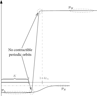
Figure 3: The Hamiltonians $L_{n}$ and $H_{n}$ with the distinguished sets of 1-periodic orbits

As in subsection 5.3.4, we obtain two short exact sequences with morphisms between them

As before, $\widehat{\operatorname*{tel}_{n}}\,CF_{+}^{*}(H_{n})$ is acyclic, $\widehat{\operatorname*{tel}_{n}}\,CF^{*}(L_{n})$ computes $SH^{*}(M)=H^{*}(M)\otimes\Lambda_{>0}$, while $\widehat{\operatorname*{tel}_{n}}\,CF_{-}^{*}(L_{n})$ computes $H^{*}(K)\otimes\Lambda_{>0}$. What is different is the map $\Phi_{L}^{H}$, which we will now show to be a quasi-isomorphism. Fix $n$ and consider the map $\Phi_{n}^{-}{:\ }CF_{-}^{*}(L_{n})\to CF_{-}^{*}(H_{n})$. Since $L_{n}\equiv H_{n}$ on $K$, the constant Floer solution sitting at a generator $x\in{\mathcal{P}}_{L}$ contributes to the continuation map and is the only energy zero connecting trajectory, therefore $\Phi_{n}^{-}(x)=x+$ terms with positive powers of $T$. This means that the reduction of $\Phi_{n}^{-}$ to the residue field is just the identity, in particular invertible, which in turn implies that $\Phi_{n}^{-}$ is invertible. Therefore the $2$-ray consisting of the complexes $CF_{-}^{*}(L_{n}),CF_{-}^{*}(H_{n})$ has the property that the maps in the finite direction are all isomorphisms. It is not hard to show that the induced map $\operatorname{tel}CF_{-}^{*}(L_{n})\to\operatorname{tel}CF_{-}^{*}(H_{n})$ is then an isomorphism, therefore so is the map on completions $\Phi_{L}^{H}{:\ }\widehat{\operatorname{tel}}_{n}CF_{-}^{*}(L_{n})\to\widehat{\operatorname{tel}}_{n}CF_{-}^{*}(H_{n})$.

Taking the homology of the right square, we arrive at the following commutative diagram:

Composing the right arrow and the inverse of the bottom arrow, we conclude that $SH^{*}(K)\cong H^{*}(K)\otimes\Lambda_{>0}$ and that under this isomorphism the restriction maps on singular and symplectic cohomologies coincide. In particular $\ker\operatorname{res}^{M}_{K}=\ker i^{*}$.

5.6 Proof of Theorem 1.54

Recall that the theorem states that if $(M,\omega)$ is symplectically aspherical, $K\subset M$ is a compact heavy set, and there is a sequence of contact-type regions $W_{i}$ with incompressible index-bounded boundary, all containing $K$ in the interior, such that $K=\bigcap_{i}W_{i}$, then for all $i$, $[\operatorname{Vol}]\in\ker\operatorname{res}^{M}_{\overline{W_{i}^{c}}}$, and in particular $[\operatorname{Vol}]\in\tau(K)=\bigcap_{i}\ker\operatorname{res}^{M}_{\overline{W_{i}^{c}}}$, therefore $K$ is SH-heavy.

For the rest of the proof we let $W$ be one of the $W_{i}$. Varolgunes proves in [27] that $SH^{*}(M)=H^{*}(M)\otimes\Lambda_{>0}$. We will prove the following

Claim 5.4.

There exists $\mu>0$ such that

$$T^{\mu}[\operatorname{Vol}]\in\ker\big{(}SH^{*}(M)\to SH^{*}(\overline{W^{c}})\big{)}\,.$$

That $[\operatorname{Vol}]\in\ker\operatorname{res}^{M}_{\overline{W^{c}}}$ follows from this upon tensoring with $\Lambda$.

Let us first recall what it means for a set to be heavy. Like in Section 5.3.1, given a ground field ${\mathbb{F}}$, the classical Floer cochain complex of a nondegenerate Hamiltonian $H$ is the ${\mathbb{F}}$-vector space $CF_{\operatorname{cl}}^{*}(H;{\mathbb{F}})={\mathbb{F}}\langle{\mathcal{P}}^{\circ}(H)\rangle$. Since the differential increases the action, for each $a\in{\mathbb{R}}$, the subspace $CF_{\operatorname{cl},\geq a}^{*}(H;{\mathbb{F}})$ generated by $x\in{\mathcal{P}}^{\circ}(H)$ with ${\mathcal{A}}_{H}(x)\geq a$ is a subcomplex. Let $HF^{*}_{\operatorname{cl},\geq a}(H;{\mathbb{F}})$ be the cohomology of $CF^{*}_{\operatorname{cl},\geq a}(H;{\mathbb{F}})$ and let $j_{a}^{*}{:\ }HF^{*}_{\operatorname{cl},\geq a}(H;{\mathbb{F}})\to HF^{*}_{\operatorname{cl}}(H;{\mathbb{F}})$ be the morphism induced by the inclusion. Letting $\operatorname{PSS}{:\ }HF^{*}_{\operatorname{cl}}(H;{\mathbb{F}})\to QH^{*}(M;{\mathbb{F}})=H^{*}(M;{\mathbb{F}})$ be the PSS isomorphism [20], we have the cohomological spectral invariants

$$c^{\vee}(A,H)=\sup\{a\in{\mathbb{R}}\,|\,A\in\operatorname{im}(\operatorname{PSS}\circ j^{*}_{a})\}\quad\text{for }A\in QH^{*}(M;{\mathbb{F}})\,.$$

The corresponding partial symplectic quasi-state $\zeta{:\ }C^{\infty}(M)\to{\mathbb{R}}$ is given by

$$\zeta(H)=\lim_{k\to\infty}\frac{c^{\vee}([\operatorname{Vol}],kH)}{k}\,,$$

where $[\operatorname{Vol}]\in H^{2n}(M;{\mathbb{F}})$ is the volume class. The original definition in [8] used homological spectral invariants $c([M],\cdot)$ relative to the fundamental class $[M]\in H_{2n}(M;{\mathbb{F}})$, but $c([M],\cdot)=c^{\vee}([\operatorname{Vol}],\cdot)$ thanks to the duality formula, see for instance [15, Section 4.2]. For $K$ to be heavy means that for each $F\in C^{\infty}(M)$ we have

$$\zeta(F)\geq\min_{K}F\,.$$

For us, the crucial consequence of the assumption that $K$ is heavy is the following

Lemma 5.5.

For any $L>0$ there exists $F\in C^{\infty}(M)$ such that $F|_{\overline{W^{c}}}<0$ and such that $c^{\vee}([\operatorname{Vol}],F)>L$.

Proof.

Let $F_{0}\in C^{\infty}(M)$ satisfy $F_{0}|_{\overline{W^{c}}}<0$ and $F_{0}|_{K}>0$. Since $K$ is heavy, we have

$$0<\min_{K}F_{0}\leq\zeta(F_{0})=\lim_{k\to\infty}\frac{c^{\vee}([\operatorname{Vol}],kF_{0})}{k}\,.$$

In particular there is $k_{0}$ such that $c^{\vee}([\operatorname{Vol}],k_{0}F_{0})>L$. Now put $F=k_{0}F_{0}$. ∎

Let us identify a neighborhood of the boundary $\Sigma=\partial W$ with the piece $\Sigma\times(1-\epsilon,1+\epsilon)_{r}$ of the symplectization of $\Sigma$, so that $\partial_{r}$ is the Liouville vector field. Let $L$ be the maximum of the actions of all the Reeb orbits on $\Sigma$, contractible in $M$, of Conley–Zehnder indices $2n-1,2n,2n+1$, and fix $F$ as in the lemma for this $L$. Then there exists an acceleration datum $(H_{i})_{i\geq 0}$ for $\overline{W^{c}}$ such that for all $i$ we have:

• $H_{i}\geq F$;

• On $W\setminus\Sigma\times(1-\epsilon,1]$, $H_{i}$ is a $C^{2}$-small Morse function plus a constant depending on $i$, and on $\overline{W^{c}}$, $H_{i}$ equals a $C^{2}$-small Morse function plus a constant depending on $i$; in particular the only $1$-periodic orbits of $H_{i}$ on $M\setminus\Sigma\times(1-\epsilon,1)$ are the critical points of these Morse functions;

• In the region $\Sigma\times(1-\epsilon,1)$, $H_{i}$ is a sufficiently small perturbation of $f_{i}\circ r$, where $f_{i}{:\ }(1-\epsilon,1)\to{\mathbb{R}}$ is a strictly decreasing smooth function;

• The $1$-periodic orbits of $H_{i}$ fall into two groups, the “upper” and the “lower” orbits; the upper orbits are situated in $W\setminus\Sigma\times(1-2\epsilon/3,1]$, and these in particular include the critical points of the Morse function $H_{i}|_{W\setminus\Sigma\times(1-\epsilon,1]}$; the “lower” orbits are in $W^{c}\cup\Sigma\times[1-\epsilon/3,1]$, and these include the critical points of the Morse function $H_{i}|_{\overline{W^{c}}}$;

• The lower orbits of $H_{i}$ of index $2n$ have actions $<L$, while all the upper orbits of index $2n$ have actions $>L$;

• There exists $c>0$ such that the minimal action of an upper orbit of $H_{i+1}$ of index $2n$ is at least $c+$ the maximal action of an upper orbit of $H_{i}$ of index $2n$.

See Figure 4 for an illustration.

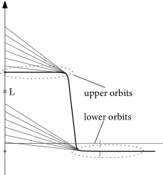
Figure 4: The action separation between the lower and upper orbits is demonstrated on the on the Hamiltonians $H_{n}$. The value $L$ is marked. The tangents whose $y$ intercepts are the actions are depicted in gray, as well as dots representing the actions of the Morse critical points.

This acceleration datum yields a $1$-ray of Floer complexes and continuation maps

$$CF^{*}(H_{0})\xrightarrow{\Phi_{H_{0}}^{H_{1}}}CF^{*}(H_{1})\to\dots$$

Lemma 5.6.

Let $y\in CF^{2n}(H_{0})$ be a linear combination of the upper orbits of $H_{0}$. Then it is killed by the composition

$$\textstyle CF^{*}(H_{0})\xrightarrow{\Phi_{H_{0}}}\varinjlim_{i}CF^{*}(H_{i})\xrightarrow{\widehat{\cdot}}\widehat{\varinjlim}_{i}CF^{*}(H_{i})\,,$$

where $\Phi_{H_{0}}$ is the natural map into the direct limit.

Proof.

The map $\Phi_{H_{0}}$ factors as follows:

$$CF^{*}(H_{0})\xrightarrow{\Phi_{H_{j-1}}^{H_{j}}\circ\dots\circ\Phi_{H_{0}}^{H_{1}}}CF^{*}(H_{j})\xrightarrow{\Phi_{H_{j}}}\varinjlim_{i}CF^{*}(H_{i})\,,$$

where $\Phi_{H_{i}}$ is again the natural map into the direct limit. By the action separation property of the acceleration datum $(H_{i})_{i}$, $\Phi_{H_{i}}^{H_{i+1}}{:\ }CF^{2n}(H_{i})\to CF^{2n}(H_{i+1})$ maps any linear combination $z$ of upper orbits of $H_{i}$ to a linear combination of upper orbits of $H_{i+1}$, since it is action-increasing. Thus $\Phi_{H_{i}}^{H_{i+1}}(z)\in T^{c}\cdot CF^{2n}(H_{i+1})$, and by induction we have

$$(\Phi_{H_{j-1}}^{H_{j}}\circ\dots\circ\Phi_{H_{0}}^{H_{1}})(y)\in T^{jc}\cdot CF^{*}(H_{j})\,,$$

whence

$$\Phi_{H_{0}}(y)=\Phi_{H_{j}}\big{(}(\Phi_{H_{j-1}}^{H_{j}}\circ\dots\circ\Phi_{H_{0}}^{H_{1}})(y)\big{)}\in T^{jc}\varinjlim_{i}CF^{*}(H_{i})$$

for all $j$, that is

$$\Phi_{H_{0}}(y)\in\bigcap_{\lambda\geq 0}T^{\lambda}\varinjlim_{i}CF^{*}(H_{i})\subset\ker\widehat{\cdot}\,.$$

∎

We now fix a $C^{2}$-small negative Morse function $G{:\ }M\to{\mathbb{R}}$, let $(s_{i})_{i\geq 0}$ be a strictly decreasing sequence of positive numbers $<1$, and put $G_{i}=s_{i}G$. Then $(G_{i})_{i\geq 0}$ is an acceleration datum for $M$. The Floer complexes $CF^{*}(G_{i})$ are all isomorphic to the Morse complex $CM^{*}(G)\otimes\Lambda_{\geq 0}$ with the differential weighted by suitable powers of $T$, while the continuation map $CF^{*}(G_{i})\to CF^{*}(G_{i+1})$ is given by $\operatorname{Crit}G\ni p\mapsto T^{G_{i+1}(p)-G_{i}(p)}p$. It follows that $\varinjlim_{i}CF^{*}(G_{i})$ is canonically isomorphic to $CM^{*}(G)\otimes\Lambda_{>0}$ with the usual Morse differential; in particular it is a complete $\Lambda_{\geq 0}$-module. The natural map $CM^{*}(G)\otimes\Lambda_{\geq 0}=CF^{*}(G_{j})\to\varinjlim_{i}CF^{*}(G_{i})=CM^{*}(G)\otimes\Lambda_{>0}$ is given by $\operatorname{Crit}G\ni p\mapsto T^{-G_{j}(p)}p$.

In particular $SH^{*}(M)=H\big{(}CM^{*}(G)\otimes\Lambda_{>0}\big{)}=HM^{*}(G)\otimes\Lambda_{>0}$ and if $q$ is a maximum of $G$, then $[\operatorname{Vol}]\otimes T^{-G_{0}(q)}\in SH^{*}(M)$ is represented by $T^{-G_{0}(q)}q\in CM^{*}(G)\otimes\Lambda_{>0}$ and is the image of $q\in CF^{*}(G_{0})$ under the natural map $CF^{*}(G_{0})\to\varinjlim_{i}CF^{*}(G_{i})$. Note that we can assume that $G_{i}\leq H_{i}$ for all $i$, therefore as in Section 4.8 there exists a filling between the acceleration data $(G_{i})_{i},(H_{i})_{i}$ and in particular we have the corresponding continuation maps $\Phi_{G_{i}}^{H_{i}}{:\ }CF^{*}(G_{i})\to CF^{*}(H_{i})$.

Lemma 5.7.

Let $q\in CF^{2n}(G_{0})$ be a maximum. Then there is $\mu\geq-G_{0}(q)$ such that $T^{\mu+G_{0}(q)}\Phi_{G_{0}}^{H_{0}}(q)$ is cohomologous in $CF^{*}(H_{0})$ to a linear combination of upper orbits.

Proof of Claim 5.4.

We have the following commutative diagram:

The middle vertical arrow comes from the $2$-ray of Floer complexes coming from the aforementioned filling. The top left arrow is the inclusion of $CF^{*}(G_{0})$ into the second direct sum in $\operatorname{tel}_{i}CF^{*}(G_{i})=\bigoplus_{i}CF^{*}(G_{i})[1]\oplus\bigoplus_{i}CF^{*}(G_{i})$, followed by completion, and similarly for the bottom left arrow. It follows that the square commutes. The top right arrow is the completion of the composition of the projection of $\operatorname{tel}_{i}CF^{*}(G_{i})$ onto $\bigoplus_{i}CF^{*}(G_{i})$ followed by the natural map into the direct limit. Varolgunes proves in [27] that this arrow is a quasi-isomorphism. The same considerations hold for the bottom right arrow. Note that the composition of the top arrows is the natural map into the direct limit, and the same is true for the composition of the bottom arrows, except the completion is then tagged on.

Fix $\mu$ as in Lemma 5.7. We will show that $T^{\mu}[\operatorname{Vol}]$ is killed by $SH^{*}(M)\to SH^{*}(\overline{W^{c}})$. The element $T^{\mu}[\operatorname{Vol}]\in SH^{2n}(M)=H^{2n}(M)\otimes\Lambda_{>0}=H^{2n}\big{(}\widehat{\operatorname{tel}}_{i}CF^{*}(G_{i})\big{)}$ is represented by the image of $T^{\mu+G_{0}(q)}q\in CF^{2n}(G_{0})$ under the top left arrow. It follows that the image of $T^{\mu}[\operatorname{Vol}]$ by $SH^{*}(M)\to SH^{*}(\overline{W^{c}})$ is represented by the image of $\Phi_{G_{0}}^{H_{0}}(T^{\mu+G_{0}(q)}q)\in CF^{2n}(H_{0})$ in $\widehat{\lim_{i}}CF^{*}(H_{i})$. By Lemma 5.7, $\Phi_{G_{0}}^{H_{0}}(T^{\mu+G_{0}(q)}q)=T^{\mu+G_{0}(q)}\Phi_{G_{0}}^{H_{0}}(q)$ is cohomologous to a linear combination of upper orbits of $H_{0}$, and thus by Lemma 5.6, this linear combination is killed by the map $CF^{*}(H_{0})\to\widehat{\lim_{i}}CF^{*}(H_{i})$. It follows that the image of $T^{\mu+G_{0}(q)}\Phi_{G_{0}}^{H_{0}}(q)$ in $\widehat{\operatorname{tel}}_{i}CF^{*}(H_{i})$ is cohomologous to zero, and thus we have our claim. ∎

Proof of Lemma 5.7.

Consider the following commutative diagram:

Here for a nondegenerate Hamiltonian $F$ we have a valuation on $CF^{*}_{\operatorname{cl}}(F;\Lambda)$ given by $T^{\lambda}x\mapsto\lambda+{\mathcal{A}}_{F}(x)$ and $CF^{*}_{\operatorname{cl},\geq 0}(F;\Lambda)$ stands for the $\Lambda_{\geq 0}$-submodule of elements with nonnegative valuation. The oblique arrows are continuation maps in respective Floer theories (classical or $T$-weighted), the upper vertical arrows are the embeddings induced by the field extension ${\mathbb{F}}\subset\Lambda$, the horizontal arrows are inclusions, while the rest of the vertial arrows are the isomorphism $\psi$ from Section 5.3.1. For instance $\psi{:\ }CF^{*}_{\operatorname{cl}}(G_{0};\Lambda)\to CF^{*}(G_{0})\otimes\Lambda$ is defined by $x\mapsto T^{{\mathcal{A}}_{G_{0}}(x)}x$, and similarly for $H_{0}$. It is easy to check that $\psi$ maps $CF^{*}_{\operatorname{cl},\geq 0}(G_{0};\Lambda)$ isomorphically onto $CF^{*}(G_{0})$ and same for $H_{0}$.

Let now $q\in CF^{2n}_{\operatorname{cl}}(G_{0};{\mathbb{F}})$ be a maximum, that is a representative of the volume class. Since continuation maps commute on cohomology with the PSS isomorphisms, it follows that $\widetilde{y}:=\Phi(q)\in CF^{2n}_{\operatorname{cl}}(H_{0};{\mathbb{F}})$ also represents the volume class, where $\Phi{:\ }CF^{*}_{\operatorname{cl}}(G_{0};{\mathbb{F}})\to CF^{*}_{\operatorname{cl}}(H_{0};{\mathbb{F}})$ is the continuation map on classical Floer cohomology. On the other hand, Lemma 5.5 and the assumption $H_{0}\geq F$ imply that $c^{\vee}([\operatorname{Vol}],H_{0})>L$, therefore there is a representative of the volume class $y\in CF^{2n}_{\operatorname{cl}}(H_{0};{\mathbb{F}})$ consisting of orbits of action $>L$, and by our choice of acceleration datum this forces $y$ to be a linear combination of the upper orbits of $H_{0}$. It follows that there is $b\in CF^{2n-1}_{\operatorname{cl}}(H_{0};{\mathbb{F}})$ such that $\widetilde{y}-y=d_{\operatorname{cl}}b$. We can now look at this equation in $CF^{*}_{\operatorname{cl}}(H_{0};\Lambda)$. The elements $\widetilde{y},b$ do not necessarily lie in $CF^{*}_{\operatorname{cl},\geq 0}(H_{0};\Lambda)$. Let $\mu\geq-G_{0}(q)>0$ be such that $T^{\mu}\widetilde{y},T^{\mu}b\in CF^{*}_{\operatorname{cl},\geq 0}(H_{0};\Lambda)$. Applying $\psi$ and noting that it is $\Lambda_{\geq 0}$-linear and commutes with continuation maps, we obtain the following equation in $CF^{*}(H_{0})$:

$$d(T^{\mu}\psi(b))=\psi(T^{\mu}\Phi(q))-\psi(T^{\mu}y)=T^{\mu}\Phi_{G_{0}}^{H_{0}}(\psi(q))-\psi(T^{\mu}y)=T^{\mu+G_{0}(q)}\Phi_{G_{0}}^{H_{0}}(q)-\psi(T^{\mu}y)\,.$$

This means that $T^{\mu+G_{0}(q)}\Phi_{G_{0}}^{H_{0}}(q)$ is cohomologous in $CF^{*}(H_{0})$ to $\psi(T^{\mu}y)$, which is a linear combination of the upper orbits of $H_{0}$, as claimed. ∎

Acknowledgments: We thank Shachar Carmeli, Liran Shaul and Moshe White for useful discussions about higher category theory, completions of modules, and combinatorial geometry, respectively. We thank Felix Schlenk for very useful remarks on the manuscript, Gleb Smirnov for pointing out that Theorem 1.17, which subsumes Theorem 1.2, is an interesting result in its own right, and Umut Varolgunes for helpful comments on Sections 1.8.2 and 1.8.3. Thanks also to Pierre-Alexandre Mailhot and Jordan Payette for pointing out a typo in the footnote of Definition 1.6.

Adi Dickstein

Tel Aviv University

School of Mathematical Sciences

69978, Tel Aviv, Israel

E-mail: adi.dickstein@gmail.com

Yaniv Ganor

Technion

Department of Mathematics

32000, Haifa, Israel

E-mail: ganory@gmail.com

Leonid Polterovich

Tel Aviv University

School of Mathematical Sciences

69978, Tel Aviv, Israel

E-mail: polterov@tauex.tau.ac.il

Frol Zapolsky

University of Haifa

Department of Mathematics

Faculty of Natural Sciences

3498838, Haifa, Israel

E-mail: frol.zapolsky@gmail.com

References

- [1] P. Biran and O. Cornea. Quantum structures for Lagrangian submanifolds. arXiv preprint arXiv:0708.4221, 2007.
- [2] M. S. Borman, N. Sheridan, and U. Varolgunes. Quantum cohomology as a deformation of symplectic cohomology. arXiv preprint arXiv:2108.08391, 2021.
- [3] R. Bott, L. W. Tu, et al. Differential forms in algebraic topology, volume 82. Springer, 1982.
- [4] K. Cieliebak and A. Oancea. Symplectic homology and the Eilenberg–Steenrod axioms. Algebraic & Geometric Topology, 18(4):1953–2130, 2018.
- [5] J. F. Davis and P. Kirk. Lecture notes in algebraic topology, volume 35. American Mathematical Soc., 2001.
- [6] H. Edelsbrunner. Algorithms in combinatorial geometry, volume 10. Springer Science & Business Media, 2012.
- [7] M. Entov and L. Polterovich. Quasi-states and symplectic intersections. Commentarii Mathematici Helvetici, 81(1):75–99, 2006.
- [8] M. Entov and L. Polterovich. Rigid subsets of symplectic manifolds. Compositio Mathematica, 145(3):773–826, 2009.
- [9] Y. Ganor and S. Tanny. Floer theory of disjointly supported Hamiltonians on symplectically aspherical manifolds. arXiv preprint arXiv:2005.11096, 2020.
- [10] J. P. Greenlees and J. P. May. Derived functors of I-adic completion and local homology. Journal of Algebra, 149(2):438–453, 1992.
- [11] M. Gromov. Singularities, expanders and topology of maps. part 1: Homology versus volume in the spaces of cycles. Geometric and Functional Analysis, 19(3):743–841, 2009.
- [12] M. Gromov. Singularities, expanders and topology of maps. part 2: From combinatorics to topology via algebraic isoperimetry. Geometric and Functional Analysis, 20(2):416–526, 2010.
- [13] R. N. Karasev. Covering dimension using toric varieties. Topology and its Applications, 177:59–65, 2014.
- [14] M. Kawasaki. Function theoretical applications of Lagrangian spectral invariants. arXiv preprint arXiv:1811.00527, 2018.
- [15] R. Leclercq and F. Zapolsky. Spectral invariants for monotone Lagrangians. Journal of Topology and Analysis, 10(03):627–700, 2018.
- [16] D. McDuff and D. Salamon. J-holomorphic curves and symplectic topology, volume 52. American Mathematical Soc., 2012.
- [17] R. S. Palais. Homotopy theory of infinite dimensional manifolds. Topology, 5(1):1–16, 1966.
- [18] J. Pardon. An algebraic approach to virtual fundamental cycles on moduli spaces of pseudo-holomorphic curves. Geometry & Topology, 20(2):779–1034, 2016.
- [19] J. Pardon. Contact homology and virtual fundamental cycles. Journal of the American Mathematical Society, 32(3):825–919, 2019.
- [20] S. Piunikhin, D. Salamon, and M. Schwarz. Symplectic Floer-Donaldson theory and quantum cohomology. In Contact and symplectic geometry, pages 171–200. Cambridge Univ. Press, Publ. Newton Instit. 8, Cambridge, 1996.
- [21] L. Polterovich, D. Rosen, K. Samvelyan, and J. Zhang. Topological persistence in geometry and analysis, volume 74. American Mathematical Soc., 2020.
- [22] R. Rado. A theorem on general measure. Journal of the London Mathematical Society, 1(4):291–300, 1946.
- [23] Y. B. Rudyak and F. Schlenk. Minimal atlases of closed symplectic manifolds. Communications in Contemporary Mathematics, 9(06):811–855, 2007.
- [24] Y. Sun. Index bounded relative symplectic cohomology. arXiv preprint arXiv:2109.06146, 2021.
- [25] D. Tonkonog and U. Varolgunes. Super-rigidity of certain skeleta using relative symplectic cohomology. arXiv preprint arXiv:2003.07486, to appear in Journal of Topology and Analysis, 2020.
- [26] U. Varolgunes. Mayer - Vietoris property for relative symplectic cohomology. Massachusetts Institute of Technology, 2018.
- [27] U. Varolgunes. Mayer–Vietoris property for relative symplectic cohomology. Geometry & Topology, 25(2):547–642, 2021.
- [28] C. A. Weibel. An introduction to homological algebra. Number 38. Cambridge university press, 1994.