Second order cumulants of conserved charge fluctuations revisited
I. Vanishing chemical potentials

Abstract

We update lattice QCD results for second order cumulants of conserved charge fluctuations and correlations at non-zero temperature and vanishing values of the conserved charge chemical potentials. We compare these results to hadron resonance gas calculations with and without excluded volume terms as well as S-matrix results in the hadronic phase of QCD, and comment on their current limitations. We, furthermore, use these results to characterize thermal conditions in the vicinity of the pseudo-critical line of the chiral transition in QCD. We argue that the ratio of strange to baryon chemical potentials is a robust observable that, on the one hand, deviates only little from hadron resonance gas results, but, on the other hand, is very sensitive to the spectrum of strange baryon resonances.

I Introduction

The thermal state of strong-interaction matter described by Quantum Chromodynamics (QCD) with two light up and down quarks and a heavier strange quark is fixed by four external control parameters, the temperature ($T$) and three chemical potentials ($\mu_{B},\mu_{Q},\mu_{S}$) that couple to the conserved currents for net baryon-number ($B$), electric-charge ($Q$) and strangeness ($S$), respectively. In a grand canonical description of equilibrium thermodynamics these external control parameters are Lagrange multiplier, appearing in the statistical operator, that characterize the thermodynamic conditions of, e.g., matter described by the strong force. The set of external parameters, ($T,\mu_{B},\mu_{Q},\mu_{S}$) may be used to calculate various bulk thermodynamic observables, e.g. energy and number densities as well as generalized susceptibilities that are obtained from higher order derivatives of the grand canonical partition function. Such observables are, in principle, measurable in experiments, while the set of Lagrange multiplier, ($T,\mu_{B},\mu_{Q},\mu_{S}$), is not. They are specific to a given model to the extent that the value of a certain bulk thermodynamic observable, e.g. the net baryon-number density, which is related to a certain temperature value $T$ in QCD (or nature) will correspond to another temperature value in a model calculation. The latter will be close to the former only when the model approximations provide a realistic description of QCD.

Lattice QCD calculations provide continuum extrapolated results for bulk thermodynamic observables at small values of the chemical potential with percent-level accuracy. This provides, in particular, the pseudo-critical temperature for the chiral transition at vanishing values of the baryon chemical potential with better than 1% accuracy Bazavov et al. (2019a) for a specific set of observables. This result differs by less than 2% from calculations using different observables and discretization schemes to characterize the crossover transition in QCD Bazavov et al. (2019a); Borsanyi et al. (2020). Similarly the temperature dependence of the pseudo-critical line, $T_{pc}(\mu_{B})$, is known with better than 2% accuracy at least for baryon chemical potentials $\mu_{B}\leq T_{pc,0}\equiv T_{pc}(0)$ Bazavov et al. (2019a); Borsanyi et al. (2020); Bonati et al. (2015). This also includes a determination of constraints on the strangeness chemical potential, $\mu_{S}(\mu_{B})$, required to insure strangeness neutrality in strongly interacting matter. At fixed value of temperature this constraint is known to better than 5% for a range of baryon chemical potentials $\mu_{B}\leq T_{pc}(\mu_{B})$.

In heavy-ion experiments at the Large Hadron Collider (LHC) and the Relativistic Heavy Ion Collider (RHIC) the thermal properties of strongly interacting matter as it existed at the time of hadronization (freeze-out of various hadrons) is probed. The underlying thermal parameters, ($T,\mu_{B},\mu_{Q},\mu_{S}$), are extracted from particle yields or higher order cumulants characterizing the distributions of these hadrons. These parameters, however, generally are not obtained through a direct comparison with QCD but with statistical models, e.g. models that use the statistical operator of hadron resonance gas (HRG) models Braun-Munzinger et al. for point-like non-interacting hadrons, which are variants of the Hagedorn resonance gas model Hagedorn (1965); Karsch and Redlich (2011); Andronic et al. (2018). This too leads to a determination of thermal parameters with errors that are on the percent level. The approach, however, may suffer from systematic uncertainties, as the statistical operator used in model calculations obviously will differ from that of QCD in certain ranges of the temperature and baryon chemical potential. Differences between the statistical operator of QCD and that of HRG models based on a spectrum of point-like, non-interacting hadron resonances become apparent in properties of higher order cumulants, e.g. deviations from (generalized) Skellam distributions that are inherent to HRG models using point-like, non-interacting hadron resonances. A proper inclusion of interactions in a hadronic medium, using a relativistic virial expansion Dashen et al. (1969); Venugopalan and Prakash (1992); Lo et al. (2013); Fernández-Ramírez et al. (2018); Andronic et al. (2019) or more phenomenology oriented excluded volume Hagedorn and Rafelski (1980a, b); Gorenstein et al. (1981); Vovchenko et al. (2017a, b); Taradiy et al. (2019) as well as repulsive mean approaches Olive (1981, 1982); Huovinen and Petreczky (2018) thus may be necessary. These approaches generally need to adjust parameters which is done by comparing to lattice QCD calculations of thermodynamic observables.

Second order cumulants can be used as important benchmark observables that allow to establish the range of validity of hadronic models that are needed to provide an interface between experimental observables, e.g. hadron yields and fluctuations, and thermal observables obtained in field theoretic calculations, e.g. QCD. In this paper we will provide high precision, continuum extrapolated lattice QCD results for second order cumulants of conserved charge fluctuations and their correlations at vanishing values of the baryon chemical potential. We will extend these calculations in a follow-up paper to non-vanishing values of the chemical potential.

The calculations presented here at vanishing values of the chemical potential allow to constrain the basic parameters that enter in model calculations, e.g. the excluded volume parameters introduced in hadron resonance gas (HRG) models to mimic the effect of repulsive interactions or the modeling of higher order corrections in S-matrix calculations that are needed to go beyond the calculation of second order coefficients in a virial expansion. Preliminary results from this study have been presented by us previously Goswami et al. (2021a, b). A similar compar- ison of lattice QCD results on cumulants of conserved charge fluctuations with excluded volume HRG models also appeared recentlyKarthein et al. (2021).

This paper is organized as follows. In the next section we describe the computational set-up for our calculations and describe the scale setting used by us to define temperature scales. Section III gives a short description of the basic observables that we analyze. Section IV describes our determination of continuum extrapolated results for all second order cumulants. Section V is devoted to a comparison of the QCD results for these cumulants with hadron resonance gas model calculations. Finally we give our conclusions in Section VI. Three appendices are devoted to the presentation of further details on the scale setting, the fits to second order cumulants and a description of differences between two lists of hadron resonances used in HRG model calculations.

II Computational set-up

The framework for our calculations with the Highly Improved Staggered Quark (HISQ) Follana et al. (2007) discretization scheme for $(2+1)$-flavor QCD with a physical strange quark mass and two degenerate, physical light quark masses is well established and has been used by us for several studies of higher order cumulants of conserved charge fluctuations and correlations. The specific set-up used in our current study has been described in Bazavov et al. (2020).

In addition to the data-sets used for that study we increased the statistics on lattices with temporal extent $N_{\tau}=12$ and $16$. This allows us to present continuum extrapolated results for all second order cumulants, for which the statistical error on the data themselves amounts to less than 50%, the reminder coming from systematic errors related to the fit ansätze used for continuum extrapolations and uncertainties on the zero temperature observables used to set the scale for the temperature.

II.1 Data sets and statistics

We follow here the notation and conventions used in Bazavov et al. (2017a) for the calculation of the equation of state in $(2+1)$-flavor QCD with non-vanishing chemical potentials. In that work first continuum extrapolated results for second order cumulants, obtained with the HISQ action, had been presented. The statistics collected for our current analysis is more than a factor 10 larger than that used in Bazavov et al. (2017a) for the calculation of the equation of state on lattices with temporal extent $N_{\tau}=8$ and $12$. Moreover, compared to the statistics used previously for a determination of the pseudo-critical temperature $T_{pc}$ of the chiral transition in $(2+1)$-flavor QCD Bazavov et al. (2019a), we increased the statistics by a factor ($3$-$4$) for existing data-sets on lattices with temporal extent $N_{\tau}=16$ in the temperature range $T\in[135~{}{\rm MeV}:178~{}{\rm MeV}]$. We also make use of data-sets obtained in earlier calculations on lattices with temporal extent $N_{\tau}=6$ Bazavov et al. (2019a, 2017a). Details on the simulation parameters and our current statistics are given in Table 1. The gauge field configurations stored in our data-sets are separated by 10 time units in a simulation with the rational Hybrid Monte Carlo (RHMC) algorithm.

$N_{\tau}=8$				$N_{\tau}=12$				$N_{\tau}=16$
$\beta$	$m_{l}$	T[MeV]	#conf.	$\beta$	$m_{l}$	T[MeV]	#conf.	$\beta$	$m_{l}$	T[MeV]	#conf.
6.175	0.003307	125.28	1,471,861
6.245	0.00307	134.84	1,275,380	6.640	0.00196	135.24	330,447	6.935	0.00145	135.80	17671
6.285	0.00293	140.62	1,598,555	6.680	0.00187	140.80	441,115	6.973	0.00139	140.86	23855
6.315	0.00281	145.11	1,559,003	6.712	0.00181	145.40	416,703	7.010	0.00132	145.95	26122
6.354	0.00270	151.14	1,286,603	6.754	0.00173	151.62	323,738	7.054	0.00129	152.19	26965
6.390	0.00257	156.92	1,602,684	6.794	0.00167	157.75	299,029	7.095	0.00124	158.21	21656
6.423	0.00248	162.39	1,437,436	6.825	0.00161	162.65	214,671	7.130	0.00119	163.50	18173
6.445	0.00241	166.14	1,186,523	6.850	0.00157	166.69	156,111	7.156	0.00116	167.53	19926
6.474	0.00234	171.19	373,644	6.880	0.00153	171.65	144,633	7.188	0.00113	172.60	17163
6.500	0.00228	175.84	294,311	6.910	0.00148	176.73	131,248	7.220	0.00110	177.80	3282

Table 1: Simulation parameters and statistics collected on lattices of size $N_{\sigma}^{3}\times N_{\tau}$ with $N_{\sigma}=4N_{\tau}$ in calculations with light to strange quark mass ratio $m_{l}/m_{s}=1/27$.

All our calculations have been performed on lattices with spatial extent $N_{\sigma}=4N_{\tau}$. Additional data on second order cumulants on lattices with temporal extent $N_{\tau}=6$ are taken from Bazavov et al. (2017a). In order to stabilize the asymptotic behavior of our fits to second order cumulants we also use data at higher temperatures, which also are taken from Bazavov et al. (2017a).

In this new analysis we focus on a temperature range of $20$ MeV above and below the pseudo-critical temperature for the chiral transition at vanishing value of the chemical potentials, $T_{pc,0}=(156.5\pm 1.5)$ MeV Bazavov et al. (2019a).

II.2 Scale setting

In order to set the scale for the temperature used in lattice QCD calculations we closely follow the strategy laid down for the definition of a line of constant physics and the calculation of the equation of state in Bazavov et al. (2014a). There we introduced temperature scales based on a calculation of $r_{1}$, which characterizes the short distance part of the heavy quark potential, and the kaon decay constant $f_{K}$. We use parametrizations of both observables to set the scale for the temperature,

$$T_{fK} = \frac{1}{N_{\tau}af_{K}}\ f_{K}\;,$$ (1)

$$T_{r1} = \left(\frac{1}{N_{\tau}}\frac{r_{1}}{a}\right)\frac{1}{r_{1}}\;.$$ (2)

The two temperature scales are related through the value of $r_{1}f_{K}$, which is solely determined through a lattice calculation, and the physical value of $r_{1}$, which requires input from experiment, e.g. the pion decay constant $f_{\pi}$. At non-zero lattice spacing the temperature scales derived from different observables differ. At finite values of the gauge coupling $\beta$ they are related through

$$\frac{T_{fK}}{T_{r1}}=\left(\frac{1}{af_{K}}\frac{a}{r_{1}}\right)r_{1}f_{K}\;.$$ (3)

The parametrizations of $a/r_{1}$ and $af_{K}$ used by us at non-vanishing lattice spacing are given in Appendix A. In all figures, that show lattice QCD results obtained at non-vanishing lattice spacing, we use, for definiteness, the temperature scale based on calculations of $af_{K}$, as has been done by us also in the past Bazavov et al. (2019b). For these figures and the continuum extrapolations at fixed temperature values we use as basic input the central value of the MILC results for $r_{1}$, i.e. $r_{1}=0.3106$ fm. The fits presented in Appendix A then fix the central value of the kaon decay constant to $f_{K}=155.7/\sqrt{2}$ MeV.

As discussed in more detail in Section IV.1, we treat the error on $r_{1}$ and $f_{K}$ as an overall systematic error on the temperature scale that will enter the final error budget in our analysis.

III First and second order moments of conserved net charge fluctuations

We focus here on a discussion of second order cumulants of conserved charge fluctuations at vanishing chemical potentials for the conserved charges of $(2+1)$-flavor QCD, i.e. net baryon-number ($B$), electric charge ($Q$) and strangeness ($S$). They are obtained from the QCD partition function, $\mathcal{Z}(T,V,\vec{\mu})$, as derivatives with respect to the associated chemical potentials $\vec{\mu}=(\mu_{B},\mu_{Q},\mu_{S})$,

$$\chi_{ijk}^{BQS}=\left.\frac{1}{VT^{3}}\frac{\partial\ln\mathcal{Z}(T,V,\vec{\mu})}{\partial\hat{\mu}_{B}^{i}\partial\hat{\mu}_{Q}^{j}\partial\hat{\mu}_{S}^{k}}\right|_{\hat{\mu}=0}\;,\;i+j+k=2\;.$$ (4)

This set of six second order cumulants are leading order terms in Taylor expansion of various thermodynamic quantities derived from Taylor expansions of the pressure of $(2+1)$-flavor QCD,

$$\frac{P}{T^{4}}=\frac{1}{VT^{3}}\ln\mathcal{Z}(T,V,\vec{\mu})=\sum_{i,j,k=0}^{\infty}\frac{\chi_{ijk}^{BQS}}{i!j!\,k!}\hat{\mu}_{B}^{i}\hat{\mu}_{Q}^{j}\hat{\mu}_{S}^{k}\;,$$ (5)

with $\hat{\mu}_{X}\equiv\mu_{X}/T$ and arbitrary natural numbers $i,j,k$. In particular, they provide the leading order expansion coefficients of mean ($n_{X}/T^{3}\equiv\chi_{1}^{X}$) and variance ($\sigma_{X}^{2}/T^{2}\equiv\chi_{2}^{X}$) of conserved charge distributions. At leading order in the chemical potentials the former are given by

$$n_{B}/T^{3} = \chi_{2}^{B}\hat{\mu}_{B}+\chi_{11}^{BS}\hat{\mu}_{S}+\chi_{11}^{BQ}\hat{\mu}_{Q}\;,$$ (6)

$$n_{Q}/T^{3} = \chi_{11}^{BQ}\hat{\mu}_{B}+\chi_{11}^{QS}\hat{\mu}_{S}+\chi_{2}^{Q}\hat{\mu}_{Q}\;,$$ (7)

$$n_{S}/T^{3} = \chi_{11}^{BS}\hat{\mu}_{B}+\chi_{2}^{S}\hat{\mu}_{S}+\chi_{11}^{QS}\hat{\mu}_{Q}\;.$$ (8)

Of particular interest, for a discussion of properties of strongly interacting matter, created in heavy ion collisions, is the case of strangeness neutral matter ($n_{S}\equiv 0$). The second order cumulants provide important information on the relation between strangeness and baryon chemical potentials in strongly interacting matter Bazavov et al. (2012a). To leading order this is given by,

$$\frac{\mu_{S}}{\mu_{B}}\equiv s_{1}(T)=-\frac{\chi_{11}^{BS}}{\chi_{2}^{S}}-\frac{\chi_{11}^{QS}}{\chi_{2}^{S}}q_{1}+{\cal O}(\hat{\mu}_{B}^{2})\;,$$ (9)

with

$$q_{1}=\frac{r\left(\chi_{2}^{B}\chi_{2}^{S}-\chi_{11}^{BS}\chi_{11}^{BS}\right)-\left(\chi_{11}^{BQ}\chi_{2}^{S}-\chi_{11}^{BS}\chi_{11}^{QS}\right)}{\left(\chi_{2}^{Q}\chi_{2}^{S}-\chi_{11}^{QS}\chi_{11}^{QS}\right)-r\left(\chi_{11}^{BQ}\chi_{2}^{S}-\chi_{11}^{BS}\chi_{11}^{QS}\right)}$$ (10)

Here $r=n_{Q}/n_{S}$. Note that in the isospin symmetric case, $r=1/2$, one has $q_{1}=0$. We will discuss Section V.1.4 the sensitivity of this ratio of chemical potentials to the hadron resonance spectrum contributing to the thermodynamics of strongly interacting matter.

IV Second order cumulants at vanishing chemical potential

IV.1 Continuum extrapolation of second order cumulants

Second order cumulants of conserved charge fluctuations and cross-correlations among them have been calculated in lattice QCD using various discretization schemes. This led to continuum extrapolated results in $(2+1)$-flavor QCD with physical (degenerate) light quark masses ($m_{u}=m_{d}$) and a physical strange quark mass ($m_{s}$) that have been presented, previously Bazavov et al. (2012b); Bellwied et al. (2020). The HotQCD Collaboration presented such results obtained in calculations with the HISQ action. Making use of recently obtained high statistics data we update here the continuum extrapolation of the second order cumulants and present fits to a set of four independent second order cumulants that are suitable for analyzing all six $2^{nd}$ order cumulants in the conserved charge ($B,Q,S$) basis as well as the ($u,d,s$) flavor basis Bazavov et al. (2017a) for the chemical potentials.

Among the six second order cumulants only four are independent at vanishing values of the chemical potential. The other two are constrained by isospin symmetry as our calculations, as well as most other lattice QCD calculations, are performed for two degenerate light up and down quarks. This leads to two constraints Bazavov et al. (2017a),

$$\chi_{2}^{S} = 2\chi_{11}^{QS}-\chi_{11}^{BS}\;\;,$$ (11)

$$\chi_{2}^{B} = 2\chi_{11}^{BQ}-\chi_{11}^{BS}\;.$$ (12)

In the quark flavor basis the four independent observables and the two constraints relate to the three diagonal and three off-diagonal cumulants for the light and strange quark number fluctuations and correlations. The two constraints merely reflect that $u$ and $d$-quark fluctuations are identical as are their correlations with the strange quarks, i.e. $\chi_{2}^{u}=\chi_{2}^{d}$ and $\chi_{11}^{us}=\chi_{11}^{ds}$. We also note that the above constraints are fulfilled to better than 1% also in HRG model calculations that utilize the experimentally determined, physical hadron resonance spectrum Zyla et al. (2020). Here small mass differences among isospin partners arise from differences in the up and down quark masses as well as electromagnetic interactions. The above constraints, of course, also hold for HRG model calculations using hadron spectra calculated e.g. within relativistic quark models Capstick and Isgur (1986); Ebert et al. (2009); Faustov and Galkin (2015) as well as for spectra obtained in lattice QCD calculations Edwards et al. (2011); Edwards (2020).

All possible second order cumulants and ratios thereof, calculated either in the ($B,Q,S)$ or $(u,d,s)$ basis for the chemical potentials Allton et al. (2005), thus can be obtained from four independent observables; we focus on the set of observables $\chi_{2}^{Q}$, $\chi_{11}^{QS}$, $\chi_{11}^{BQ}$, $\chi_{11}^{BS}$. While the first two cumulants are dominated by contributions from the non-strange ($\chi_{2}^{Q}$) and strange ($\chi_{11}^{QS}$) meson spectrum the latter two are dominated by the non-strange ($\chi_{11}^{BQ}$) and strange ($\chi_{11}^{BS}$) baryon sectors of the hadron spectrum.

The second order cumulants have been obtained in recent high statistics calculations on lattices with temporal extent $N_{\tau}=8,\ 12,\ 16$ that focused on a calculation of higher order cumulants Bazavov et al. (2020, 2017b). These calculations have been extended, focusing on the temperature range in the vicinity of the pseudo-critical temperature, $T_{pc,0}$, for the chiral transition. The current statistics, accumulated in these calculations, is given in Table 1. Moreover, we used data sets obtained earlier on lattices with temporal extent $N_{\tau}=6$ Bazavov et al. (2019a, 2017a). For each $N_{\tau}$ we used cubic spline interpolations of our data in the interval $T\in[134~{}{\rm MeV}:178~{}{\rm MeV}]$ (see Appendix B). These interpolations allow us to obtain for each of the four different lattice sizes cumulants at the same temperature. This has been done for each of the two schemes used to define a temperature scale at non-vanishing values of the lattice spacing.

Continuum extrapolations of these observables have been performed in both schemes, using linear and quadratic extrapolations in $1/N_{\tau}^{2}$,

$$f_{2}(T,N_{\tau}) = f_{2}(T)+\frac{a_{2}}{N_{\tau}^{2}}\;,$$ (13)

$$f_{4}(T,N_{\tau}) = f_{4}(T)+\frac{b_{2}}{N_{\tau}^{2}}+\frac{b_{4}}{N_{\tau}^{4}}\;.$$ (14)

For some temperature values the linear and quadratic extrapolations are shown in Appendix B. Results obtained with linear extrapolations on the $N_{\tau}=8,\ 12,\ 16$ data sets based on the $r_{1}$ and $f_{K}$ temperature scales are compared in Fig. 1.

Differences in the continuum extrapolation shown in Fig. 1, that arise from the usage of two different temperature scales, reflect systematic errors arising from the parametrization of $a/r_{1}$ and $af_{K}$ at finite values of the gauge coupling. Moreover, the restriction to linear fit ansätze reacts differently to truncated higher order corrections in both schemes. Our final continuum extrapolation result for second order cumulants is obtained by averaging over the two different linear fit results. The difference in the two extrapolations at each temperature is taken as a systematic error and has been added linearly to the statistical errors of the two extrapolations based on the $r_{1}$ and $f_{K}$ temperature scales, respectively. Further details on our continuum extrapolations are given in Appendix B.

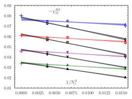
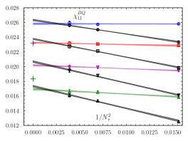
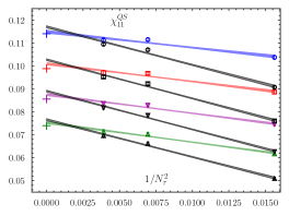
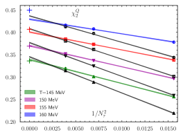
Figure 1: Continuum limit extrapolations for the cumulants $\chi_{11}^{BS}$ (top, left), $\chi_{11}^{BQ}$ (top, right), $\chi_{11}^{QS}$ (bottom, left) and $\chi_{2}^{Q}$ (bottom, right) at several values of the temperature, which has been obtained from $af_{K}$ (colored lines) and $a/r_{1}$ (black lines), respectively. Extrapolations are linear in $1/N_{\tau}^{2}$ and for data obtained on lattices with temporal extent $N_{\tau}=8,\ 12,\ 16$. Crosses indicate the corresponding QMHRG2020 value at that temperature. Note that for $\chi_{11}^{BQ}$ and $\chi_{2}^{Q}$ these HRG results are not shown for all temperature values as the deviations from the corresponding QCD results are too large. For $\chi_{2}^{Q}$ QMHRG2020 with the finite-volume corrected contributions for pions and kaons in a volume $LT\equiv N_{\sigma}/N_{\tau}=4$ has been used (see Section V.2).

The presentation of the continuum extrapolations in Fig. 1 makes use of a specific choice for the value of $r_{1}$ to define the temperature scale, i.e. we used $r_{1}=0.3106$ fm, which is the central value for $r_{1}$ quoted by the MILC Collaboration Bazavov et al. (2010), $r_{1}=0.3106(8)(14)(4)$ fm. Here the errors are statistical, systematic and experimental, respectively. The statistical error and part of the systematic error on the value for $r_{1}$, quoted by the MILC collaboration, corresponds to errors also arising in our calculation when analyzing results obtained with two different $T$-scales, different fit ansätze and fit ranges used for the continuum extrapolations.

In addition to this error we obviously need to add the systematic uncertainty in the $T$-scale arising from the error on the experimental value of the pion decay constant, $f_{\pi}$, quoted by MILC as $\Delta r_{1}=0.0004$ fm. This gives rise to an uncertainty of the $T$-scale of about $0.2$ MeV in the $T$-range considered by us. There also is a substantial spread in values for $r_{1}$ obtained by several groups and quoted by FLAG Aoki et al. (2020), for instance in Table 56. We estimate this overall systematic uncertainty on $r_{1}$ as $\Delta r_{1}=0.001$ fm, which for the temperature range considered by us amounts to a scale uncertainty of $\Delta T\simeq 0.6$ MeV. The resulting systematic error is shown separately for all our continuum extrapolated results on second order cumulants.

Continuum extrapolated results for all four independent second order cumulants, calculated on lattices with temporal extent $N_{\tau}=6,\ 8,\ 12$ and $16$ are shown in Fig. 2 in the temperature range $130~{}{\rm MeV}<T<180~{}{\rm MeV}$. In that figure we also show separately the systematic error arising from the scale uncertainties discussed in the previous paragraph (red band), and the combined statistical and systematic error arising from the continuum extrapolation using two different $T$-scales (grey band). The insets in these figures show a comparison between the lattice QCD results and a specific HRG model calculation that is based on the QMHRG2020 list of resonances (see Section V.1.1). This will be discussed further in the next section.

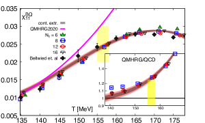
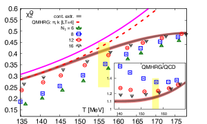
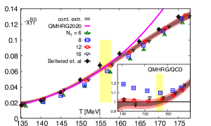
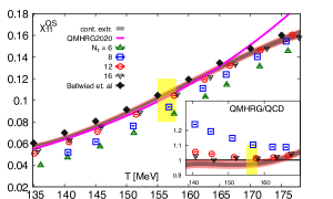
Figure 2: Four independent second order cumulants versus temperature calculated on lattices with different temporal extent $N_{\tau}$. Lines show results from HRG model calculations using point-like, non-interacting resonances and the hadron spectrum list QMHRG2020 discussed in Section V.1.1. The insets show the ratio of continuum extrapolated lattice QCD results and HRG model calculations based on QMHRG2020. Also shown are results from Bellwied et al. Bellwied et al. (2020). For the presentation of data at finite values of $N_{\tau}$ the temperature scale based on calculations of $af_{K}$ has been used. Here and in all other figures the yellow band corresponds to the crossover temperature, $T_{pc,0}$.

The uncertainty of the $T$-scale determination has been propagated into a systematic error for our continuum extrapolated observables at temperature $T$. This is quoted as a systematic error on the observables at temperature $T$. Results for some values of the temperature are given in Table 2 and compared with corresponding results obtained in Ref. Bellwied et al. (2020). As can be seen agreement between these two analyses is quite good.

$T[\rm MeV]$	$\chi_{11}^{BQ}$		$\chi_{11}^{BS}$		$\chi_{11}^{QS}$		$(\chi_{2}^{Q})_{LT=4}$
	this work	Bellwied et al. (2020)	this work	Bellwied et al. (2020)	this work	Bellwied et al. (2020)	this work
135	0.0114(5)(2)	0.0101(8)	-0.0197(15)(3)	-0.0167(17)	0.0576(13)(6)	0.0604(20)	0.285(4)(2)
140	0.0140(4)(3)	0.0124(8)	-0.0251(7)(7)	-0.0227(13)	0.0655(10)(9)	0.0699(18)	0.312(4)(3)
145	0.0172(4)(3)	0.0162(12)	-0.0345(8)(11)	-0.0332(18)	0.0760(12)(12)	0.0806(20)	0.342(4)(3)
150	0.0204(4)(3)	0.0217(17)	-0.0469(10)(14)	-0.0491(28)	0.0883(12)(13)	0.0914(12)	0.374(5)(3)
155	0.0235(4)(3)	0.0242(10)	-0.0616(14)(15)	-0.0676(38)	0.1018(14)(14)	0.1045(9)	0.404(5)(3)
160	0.0261(4)(2)	0.0266(7)	-0.0775(20)(16)	-0.0825(27)	0.1160(16)(14)	0.1193(15)	0.433(5)(3)
165	0.0280(3)(1)	0.0278(6)	-0.0938(22)(15)	-0.0981(26)	0.1300(18)(14)	0.1345(20)	0.458(5)(2)
170	0.0288(2)(0)	0.0277(4)	-0.1097(24)(14)	-0.1136(23)	0.1434(20)(12)	0.1478(22)	0.476(4)(1)
175	0.0281(3)(1)	0.0269(4)	-0.1244(30)(12)	-0.1296(24)	0.1553(26)(12)	0.1600(23)	0.489(4)(1)

Table 2: Continuum extrapolated results for the set of four independent second order cumulants obtained at some values of $T$. The second error given for our data corresponds to the uncertainty in the physical value of $r_{1}$ as discussed in the text. In the case of $\chi_{2}^{Q}$ we explicitly indicate that these results are sensitive to finite volume effects and have been obtained on lattices with aspect ratio $LT\equiv N_{\sigma}/N_{\tau}=4$ (see discussion in Section V.2). Also shown are results from Bellwied et al. Bellwied et al. (2020).

Further details on our continuum extrapolated results and comparisons with various HRG model calculations as well as results obtained from virial expansions will be presented in the next sections.

IV.2 Parametrization of the continuum extrapolated second order cumulants

When performing the continuum extrapolations of second order cumulants we did not assume any specific ansatz for the temperature dependence of the cumulants. It, however, will be useful also for comparisons with other observables and model calculations to have at hand a parametrization of the four independent second order cumulants as well as the two dependent observables, $\chi_{2}^{B}$ and $\chi_{2}^{S}$. For this purpose we provide a parametrization in terms of rational polynomials,

$$\chi_{11}^{XY}(T)=\frac{\sum\limits_{k=0}^{3}n_{k}^{XY}\bar{t}^{k}}{1+\sum\limits_{k=1}^{3}d_{k}^{XY}\bar{t}^{k}}\;,\;\bar{t}=\left(1-\frac{T_{pc,0}}{T}\right)~{}\;,$$ (15)

where $X,Y\in{B,Q,S}$, and it is understood that $\chi_{11}^{XY}$ should be replaced by $\chi_{2}^{X}$ for $X=Y$. This parametrization corresponds to the center of the error bands shown in Fig. 2. The coefficients for these parametrizations are given in Table 3.

	$\chi^{BQ}_{11}$	$\chi^{QS}_{11}$	$\chi^{BS}_{11}$	$\chi^{Q}_{2}$	$\chi^{B}_{2}$	$\chi^{S}_{2}$
$n^{XY}_{0}$	0.0243	0.106	-0.066	0.413	0.115	0.279
$n^{XY}_{1}$	0.0122	0.0629	-0.327	-0.159	0.328	-1.172
$n^{XY}_{2}$	-0.376	-0.6097	0.0290	-2.099	-0.933	-6.661
$n^{XY}_{3}$	-1.219	-3.896	3.834	-6.362	-6.522	-28.378
$d^{XY}_{1}$	-3.036	-3.572	-2.505	-2.605	-2.922	-9.135
$d^{XY}_{2}$	3.006	3.166	2.952	1.677	3.189	13.624
$d^{XY}_{3}$	-2.133	-5.080	3.0973	3.892	-0.245	-66.402

Table 3: Parametrization of second order cumulants representing lines for central values of the fits shown in Fig. 2 in the interval $T\in[135~{}{\rm MeV}:175~{}{\rm MeV}]$.

As a consistency check we use the parametrizations of the four independent cumulants and compare with the diagonal susceptibilities $\chi_{2}^{S}$ and $\chi_{2}^{B}$, respectively. Note that for fixed $N_{\tau}$ these data fulfill exactly the constraints given in Eqs. 11 and 12. The data for $\chi_{11}^{BQ}$, $\chi_{11}^{BS}$ and $\chi_{11}^{QS}$, however, are correlated, which may lead to slight differences in the continuum extrapolated results. We show the continuum extrapolations for $\chi_{2}^{B}$ and $\chi_{2}^{S}$ in Fig. 3. Here the error band has been obtained in the same way as for the off-diagonal cumulants. The continuum extrapolated results for these diagonal second order cumulants are given in Table 4 for the same temperature values as those given in Table 2 for the set of four independent second order cumulants. Although the continuum extrapolated results for $\chi_{2}^{B}$ and $\chi_{2}^{S}$ have been obtained without imposing explicitly the relations given in Eqs. 11 and 12 we find that the continuum extrapolated cumulants are consistent with these constraints within errors and also the parametrization of second order cumulants given in Table 3 do so to better than 1%.

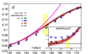
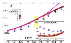
Figure 3: The diagonal second order cumulants $\chi_{2}^{B}$ (left) and $\chi_{2}^{S}$ (right) versus temperature calculated on lattices with different temporal extent $N_{\tau}$. Lines show results from HRG model calculations using point-like, non-interacting resonances and the hadron spectrum list QMHRG202, introduced in Section V.1.1. The insets show the ratio of continuum extrapolated lattice QCD results and the HRG model calculations based on QMHRG2020.

$T[\rm MeV]$	$\chi_{2}^{B}$	$\chi_{2}^{S}$
135	0.0422(22)(10)	0.134(4)(2)
140	0.0532(14)(14)	0.156(2)(2)
145	0.0689(15)(18)	0.187(3)(3)
150	0.0878(18)(20)	0.224(3)(4)
155	0.1085(22)(21)	0.266(4)(4)
160	0.1296(26)(21)	0.310(5)(4)
165	0.1497(28)(19)	0.354(6)(4)
170	0.1673(27)(15)	0.396(7)(4)
175	0.1809(29)(11)	0.435(8)(4)

Table 4: Continuum extrapolated results for $\chi_{2}^{B}$ and $\chi_{2}^{S}$ obtained at some values of $T$. The second error reflects the uncertainty in the value of $r_{1}$ used for setting the temperature scale as discussed in the text.

V Second order cumulants in QCD and the hadron resonance gas model

In this section we compare QCD results for second order cumulants with HRG model calculations. We will discuss the importance of additional resonances contributing to correlations of net strangeness fluctuations with net baryon-number and net electric-charge fluctuations, respectively. We also discuss in detail the quite different behavior of correlations between net baryon-number and net electric-charge fluctuations on the one hand and net baryon-number and net strangeness fluctuation on the other hand, which is apparent when comparing QCD and HRG model calculations. Furthermore, we comment on the significance of finite volume effects visible in the second order cumulant of net electric-charge fluctuations.

V.1 Sensitivity of second order cumulants to details of the hadron resonance gas spectrum

Obviously, conclusions drawn from a comparison of HRG model calculations with QCD results crucially depend on the hadron spectrum which is input to the HRG model calculations. Although such models can rely on a lot of information from experimentally determined resonances Zyla et al. (2020), it has been noted that this information is not sufficient to constrain interactions in a hadron resonance gas to such an extent that these models do provide satisfactory comparisons with QCD results. As noted earlier Bazavov et al. (2014b), in particular in the baryon sector of the spectrum additional strange hadron resonances seem to be needed to obtain reasonable agreement between HRG model calculations and QCD results for strangeness fluctuations and their correlations with electric charge and baryon number fluctuations, respectively.

In particular, when using in HRG model calculations with point-like, non-interacting resonances only well established mesons and 3- and 4-star baryon resonances listed in the summary tables of the particle data group (PDG) Zyla et al. (2020), the comparison with QCD results yields only poor agreement in the strangeness sector (see Fig. 4 (top)). Including additional resonances that have been predicted in QCD based quark model (QM) calculations, e.g. in Capstick and Isgur (1986); Ebert et al. (2009); Faustov and Galkin (2015), as well as lattice QCD calculations Edwards et al. (2011); Edwards (2020), significantly improves the comparison between HRG model and QCD calculations. However, such an approach is not unique. It depends on details of the relativistic quark model calculations (for a recent compilation of results see Menapara and Rai (2021)) as well as the treatment of the not well established resonances listed by the PDG. Moreover, it is well understood since the early work of Hagedorn Hagedorn (1965) and Dashen, Ma and Bernstein Dashen et al. (1969) that a modeling of strong interactions in terms of point-like, interacting resonances is not sufficient to account for all interactions in strongly interacting matter. The need for a proper treatment of additional repulsive interactions, for instance by assigning an intrinsic volume to each hadron, has been pointed out early on Hagedorn and Rafelski (1980a, b). However, it also has been noted that at the same time the interplay between repulsive and attractive interaction needs to be taken into account.

A more rigorous treatment of interactions among hadrons in medium can be achieved in the S-matrix formalism Dashen et al. (1969) which is the starting point for a systematic virial expansion of relativistic quantum gases Fiore et al. (1977); Venugopalan and Prakash (1992). The subtle interplay of attractive and repulsive interactions is, at least in principle, taken care of in the virial expansion. In the case of the strange meson $K_{0}^{*}(700)$, for instance, an analysis of the effect of attractive and repulsive contributions in the S-matrix, partial wave analysis led to the conclusion that the contribution of this resonance to the thermodynamics of strong interaction matter is strongly suppressed. Effectively it does not contribute at all and the resonance thus should not be included in point-like, non-interacting HRG models Broniowski et al. (2015); Friman et al. (2015), despite the fact that it is listed as a well established resonance in the PDG tables.

Setting up a HRG model for the description of the thermodynamics of strong interaction matter in the low temperature, hadronic regime thus is subject to a certain amount of ambiguity. Nonetheless, such models are a good starting point for the comparison to QCD calculations and can serve as a mediator between QCD calculations and experimental observations.

V.1.1 QMHRG2020

Previously we used a list of hadron resonances (QMHRG) that included only established mesons and 3- and 4-star baryon resonances listed in the PDG summary tables and had been augmented with a list of QM states in the strange and non-strange baryon sectors Bazavov et al. (2014b). We now updated this list of hadron resonances by taking into account the 1- and 2-star baryon resonances as well as mesons not listed as being well established in the PDG 2020 summary tables Zyla et al. (2020). We, however, left out the $K_{0}^{*}(700)$ (see below). This defines the list of hadron resonances, QMHRG2020.

To a large extent the resonances, listed in the PDG tables, have counterparts in the hadron spectrum calculated in relativistic quark models Capstick and Isgur (1986); Ebert et al. (2009); Faustov and Galkin (2015). In order to avoid double counting we used from the QM calculations only states that have no identified counterparts in the PDG tables. QMHRG2020 differs from the QMHRG2016+ list Alba et al. (2017) by only a few resonances. In the strange baryon sector this leads to a few percent differences in the HRG model calculation of $\chi_{11}^{BS}$, that are of significance when comparing HRG model calculations with QCD results, while in all other cases differences in the two lists are negligible. For instance, for temperatures below the QCD pseudo-critical temperature, i.e. for $T\sim(140-155)$ MeV, HRG model results for $\chi_{11}^{BS}$, obtained from both lists, differ by about 6%. Eliminating the QM counterparts Capstick and Isgur (1986); Faustov and Galkin (2015) of two 4-star as well as two 3-star resonances from the QMHRG2016+ list reduces this difference to 3%. In Table 6 of Appendix C we give a list of 8 strange baryon resonances that are listed in the PDG tables and also have been calculated in relativistic quark models. Eliminating the latter from QMHRG2016+ reproduces results obtained with QMHRG2020 within 1% accuracy.

In the following we use the QMHRG2020 list of hadron resonances as baseline model for comparisons with QCD calculations. In the insets of Fig. 2 we have compared the continuum extrapolated results for four independent second order cumulants, obtained in $(2+1)$-flavor QCD, with HRG model calculations that make use of the QMHRG2020 list. The insets show the ratio of results obtained in HRG model calculations and QCD, respectively. As can be seen, at low temperatures the agreement is fairly good. In detail, however, the differences seen in QCD and HRG model calculations are quite different for the four second order cumulants and reflect different physics. We will discuss this in more detail in the following subsections. We note already here that the difference between QCD results and HRG calculations is particularly striking for correlations between net baryon-number and electric charge, $\chi_{11}^{BQ}$.

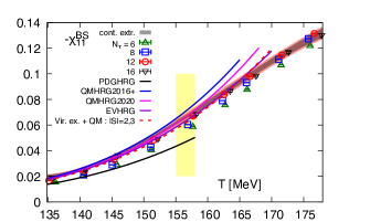
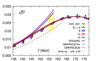
Figure 4: Continuum extrapolated results for $\chi_{11}^{BS}$ (top) and $\chi_{11}^{BQ}$ (bottom). Shown is a comparison to HRG model calculations based on different lists for hadron resonances as discussed in the text. Also shown are results obtained with excluded volume HRG models, using an excluded volume parameter $b=0.4$ fm³, and virial expansions Lo et al. (2018); Fernández-Ramírez et al. (2018), respectively.

V.1.2 Net baryon-number fluctuations and correlations

In Fig. 4 we compare HRG model calculations using different hadron resonance spectra with continuum extrapolated lattice QCD results for (2+1)-flavor QCD. As can be seen correlations between net baryon-number and strangeness fluctuations ($\chi_{11}^{BS}$) are particularly sensitive to contributions from the strange baryon resonances, while correlations between net baryon-number and electric charge fluctuations ($\chi_{11}^{BQ}$) show only little sensitivity to contributions from additional baryon resonances; this cumulant only depends mildly on the strange baryon sector as only $|S|=2,3$ baryons contribute to $\chi_{11}^{BQ}$. The small differences seen in the magnitude of $\chi_{11}^{BQ}$ when calculated with PDGHRG and QMHRG spectra, respectively, (Fig. 4 (bottom)) mainly arise from additional non-strange baryons obtained in QM calculations.

We note that $|\chi_{11}^{BS}|$, calculated in a HRG model using QMHRG2020, is larger by about 30% relative to calculations based only on 3- and 4-star resonances listed by the PDG. HRG model calculations of $\chi_{11}^{BS}$, using QMHRG2020, are consistent with QCD results at and below the pseudo-critical temperature. HRG model results for $\chi_{11}^{BQ}$, on the other hand, are clearly larger than the corresponding QCD results for temperatures $T\raise 1.29167pt\hbox{$>$\kern-7.5pt\raise-4.73611pt\hbox{$\sim$}}145$ MeV. They are about 20% larger at $T_{pc,0}$. This is a quite robust result, as HRG model calculations for $\chi_{11}^{BQ}$ are not very sensitive to the details of the HRG resonance spectrum used and even the inclusion of 1- and 2-star resonances has little effect, as can be seen in Fig. 4 (bottom).

In the case of net baryon-number fluctuations, $\chi_{2}^{B}$, which are related to $\chi_{11}^{BQ}$ and $\chi_{11}^{BS}$ through Eq. 12, this still leads to 10% larger results in HRG model calculations than QCD results obtained at $T_{pc,0}$.

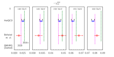
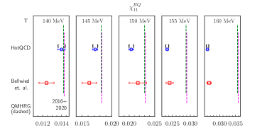
Figure 5: Comparison of continuum extrapolated lattice QCD results for the second order cumulants $\chi_{11}^{BS}$ (left) and $\chi_{11}^{BQ}$ (right) with QMHRG model calculations based on the QMHRG2020 and QMHRG2016+ list of hadron resonances. In addition to the results from this work (HotQCD) we also show results from Bellwied et al. Bellwied et al. (2020). For our results we show separately statistical errors and systematic errors (brackets) arising from the systematic error on $r_{1}$.

In Fig. 5 we show for temperatures close to and below $T_{pc,0}$ a comparison between HRG model calculations, performed with the QMHRG2020 and QMHRG2016+ resonance lists, and QCD. In this figure we also compare our results with results obtained by Bellwied et al. Bellwied et al. (2020). Within the current statistical and systematic uncertainties the results of both works are consistent with each other.

As outlined above, the larger magnitude obtained for $|\chi_{11}^{BS}|$ when using QMHRG2016+ arises from the fact that this list uses some quark model states that are also listed in the PDG tables. As a consequence the HRG model contains too many strange baryons; QMHRG2020 gives better agreement with QCD results below $T_{pc,0}$.

The differences between lattice QCD calculations and HRG model calculations using point-like, non-interacting hadronic resonances, indicate that these models do not correctly reflect interactions in a strongly interacting medium. It has been attempted to improve the model calculations by taking into account additional repulsive interactions in so-called excluded volume HRG models (EVHRG) Gorenstein et al. (1981); Vovchenko et al. (2017a); Taradiy et al. (2019). Generically the magnitude of second order cumulants involving net baryon-number fluctuations is decreased in such excluded volume HRG models. Indeed, in the case of $\chi_{11}^{BQ}$ this may improve the comparison to QCD. However, at the same time it is obvious that EVHRG model calculations for $\chi_{11}^{BS}$ will spoil the good agreement observed between QCD results and HRG model calculations with point-like, non-interacting resonances observed below $T_{pc,0}$. While $\chi_{11}^{BS}$ favors only small excluded volumes, $\chi_{11}^{BQ}$ would require large volumes to achieve agreement between HRG model calculations and QCD results.

In fact, the relative change in second order cumulants involving net baryon-number fluctuations, calculated in HRG and EVHRG models, respectively, is identical Taradiy et al. (2019)

$$R_{B}^{EV} = \frac{(\chi_{11}^{BQ})_{EVHRG}}{(\chi_{11}^{BQ})_{HRG}}=\frac{(\chi_{11}^{BS})_{EVHRG}}{(\chi_{11}^{BS})_{HRG}}=\frac{(\chi_{2}^{B})_{EVHRG}}{(\chi_{2}^{B})_{HRG}}$$ (16)

$$= 1-2bP_{B}^{HRG}(T)/T+{\cal O}(b^{2})\;.$$

Here $b$ parametrizes the size of the excluded volume for all baryons and $P_{B}^{HRG}(T)$ denotes the contribution of baryons and anti-baryons to the pressure in a resonance gas model for non-interacting point-like resonances. It contains all information on details of the hadron spectrum. The excluded volume parameter $b$ is related to the hard-sphere radius ($r$) of a hadron through $b=16\pi r^{3}/3$.

The comparison of EVHRG model calculations and QCD results, shown in Figs. 4 and 5 for $\chi_{11}^{BS}$ and $\chi_{11}^{BQ}$, makes it clear that no unique choice for $b$ exists that would give better agreement between QCD and HRG models for both cumulants simultaneously. In fact, using Eq. 16 we may write

$$\frac{(\chi_{11}^{BX})_{EVHRG}}{(\chi_{11}^{BX})_{QCD}}=R_{B}^{EV}\frac{(\chi_{11}^{BX})_{HRG}}{(\chi_{11}^{BX})_{QCD}}\;\;,\;\;X=Q,\ S.$$ (17)

Within the errors put on QCD results, this ratio should be consistent with unity for EVHRG models in order to be consistent with QCD results. This puts bounds on the magnitude of the excluded volume parameter $b$. Using the QCD result for $\chi_{11}^{BX}$, $X=S,\ Q$, and including the combined statistical and systematic error $\Delta_{X}$, we find the largest ($b^{+}$) and smallest ($b^{-}$) excluded volume parameters that would yield EVHRG model results consistent with QCD results,

$$b^{\pm}=\frac{1}{2T^{3}(\chi_{2}^{B})_{HRG}}\left(1-\frac{(\chi_{11}^{BX}\pm\Delta_{X})_{QCD}}{(\chi_{11}^{BX})_{HRG}}\right)\;\;.\;\;$$ (18)

Here we used the relation between the baryonic part of the pressure and the second order cumulant of net baryon-number fluctuations in HRG models with point-like hadrons, $P_{B}/T^{4}=\chi_{2}^{B}$. At low temperatures these bounds are not very stringent as the hadronic medium is dilute. However, close to $T_{pc,0}$, i.e. for $T=(150-155)$ MeV, we find that $b\leq 0.4$ fm³ is needed in order for EVHRG calculations to be consistent with QCD results for $\chi_{11}^{BS}$, whereas from $\chi_{11}^{BQ}$ we find that $b$ should be significantly larger, i.e. $1~{}{\rm fm}^{3}\leq b\leq 2~{}{\rm fm}^{3}$.

In fact, the temperature dependence of $\chi_{11}^{BQ}$ favors $b\simeq 2$ fm³. As can be seen in Fig. 2 (top, left), in QCD calculations it is found that $\chi_{11}^{BQ}$ rises much more slowly with temperature than in HRG model calculations using QMHRG2020. A value of $b$, significantly larger than $1$ fm³ would be needed to account for this difference. In Fig. 6 we show results for the temperature derivative of $\chi_{11}^{BQ}$ shown in Fig. 2 (top, left). In the case of QCD these derivatives are obtained from the parametrization given in Eq. 15, using a bootstrap fit to the continuum extrapolated results shown in Fig. 2. As can be seen $b\raise 1.29167pt\hbox{$>$\kern-7.5pt\raise-4.73611pt\hbox{$\sim$}}2$ fm³ would be needed in an EVHRG calculation to reproduce the QCD results for the temperature derivative of $\chi_{11}^{BQ}$.

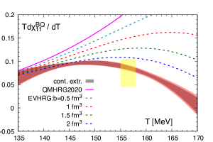
Figure 6: Temperature derivative of second order cumulant $\chi_{11}^{BQ}$ obtained in QCD (band). This result is compared to EVHRG calculations using the QMHRG2020 and several values of the excluded volume parameter $b$.

As excluded volume corrections are identical for all baryon correlations and fluctuations, it is instructive to look at ratios of second order cumulants involving net baryon-number fluctuations. In this case excluded volume corrections drop out. Any difference between HRG and QCD cumulants thus is of different origin. We also note that due to the relation given in Eq. 12, it suffices to analyze one ratio, e.g. $\chi_{11}^{BQ}/\chi_{11}^{BS}$. Other ratios, are then simply related to this ratio, e.g.,

$$\frac{\chi_{2}^{B}}{\chi_{11}^{BS}} = 2\frac{\chi_{11}^{BQ}}{\chi_{11}^{BS}}-1\;,$$

$$\frac{\chi_{2}^{B}}{\chi_{11}^{BQ}} = 2-\frac{\chi_{11}^{BS}}{\chi_{11}^{BQ}}\;.$$ (19)

Differences found between QCD and HRG model calculations of $\chi_{11}^{BQ}/\chi_{11}^{BS}$ thus translate into corresponding differences for the other two ratios. Results for $\chi_{11}^{BQ}/\chi_{11}^{BS}$ are presented in Fig. 7. This shows that deviations from HRG model calculations, which cannot be accounted for in excluded volume models using a single parameter $b$, become significant already at temperatures $T\simeq 145$ MeV. This, of course, is a direct consequence of the deviation of HRG model calculations from QCD results setting in for $\chi_{11}^{BQ}$ already at $T\simeq 140$ MeV, while at the same time results for $\chi_{11}^{BS}$ obtained in HRG model calculations are in good agreement with QCD up to $T_{pc,0}$.

A similar conclusion has been drawn from calculations of the second virial coefficients using the S-matrix approach Lo et al. (2017), where it has been pointed out that the influence of repulsive interactions, which motivated an excluded volume ansatz, is subtle and quite different in various quantum number channels contributing in the partial wave analysis of the second virial expansion coefficient.

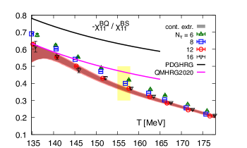
Figure 7: Ratio of continuum extrapolated lattice QCD results for $\chi_{11}^{BQ}$ and $\chi_{11}^{BS}$ versus temperature.

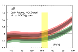
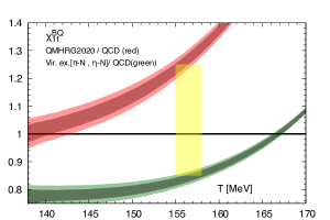
Figure 8: Comparison of continuum extrapolated lattice QCD results for $\chi_{11}^{BS}$ (top) and $\chi_{11}^{BQ}$ (bottom) with HRG model results based on QMHRG2020 (red band) and second order virial expansion results (green band) Lo et al. (2018); Fernández-Ramírez et al. (2018).

Although the S-matrix approach, which is based on experimental information on phase shifts contributing to the S-matrix, provides a rigorous formulation of the thermodynamics of an interacting hadron gas in the grand canonical ensemble and, at least in principle, does not require any a-priori information on a particular spectrum of resonances, it generally is difficult to arrive at first principle, quantitative results on properties of second order cumulants. In a systematic virial expansion of the partition function, expressed in terms of the S-matrix, even the calculation of the second virial coefficient often suffers from insufficient experimental information even for two-particle interactions. Moreover, at higher densities multi-particle interactions become of importance Dashen et al. (1969); Venugopalan and Prakash (1992), which are poorly known and thus require approximations when comparing a S-matrix based analysis to e.g. first principle lattice QCD calculations Lo et al. (2013); Fernández-Ramírez et al. (2018); Andronic et al. (2019).

In Fig. 8 we compare QCD results for second order cumulants involving net baryon-number fluctuations, with corresponding results from calculations of the second virial coefficient. In Ref. Fernández-Ramírez et al. (2018) the second virial coefficient for the description of correlations between net baryon-number and net strangeness fluctuation has been obtained in a unitary, multi-channel analysis Capstick and Roberts (1994); Hunt and Manley (2019). We show results from this analysis in Fig. 8 (top). As can be seen, agreement between S-matrix calculations and lattice QCD results is within (10-15)% below the pseudo-critical temperature. This result is similar to, but does at present not improve over results that can already be achieved within a HRG model calculation based on QMHRG2020.

A calculation of the second virial coefficient for the description of correlations between net baryon-number and net electric-charge fluctuations is more difficult as less information on the relevant interaction channels is known. In Lo et al. (2018) $\chi_{11}^{BQ}$ has been analyzed in the S-matrix approach taking into account two body interactions arising from elastic $\pi$-$N$ scattering, and a small contribution from the inelastic $\pi$-$N\rightarrow\eta$-$N$ channel. This partial calculation of the second virial expansion coefficient turns out not to be sufficient to achieve good agreement with QCD results Lo et al. (2018); Andronic et al. (2019). Although it improves the comparison with QCD, deviations at low temperatures are about a factor two larger than in the S-matrix analysis of $\chi_{11}^{BS}$. The inclusion of further interaction channels and contributions from higher order corrections clearly is needed.

At present the insufficient knowledge on scattering process contributing to $\chi_{11}^{BQ}$ can only be overcome by modeling contributions from three body and higher order interactions. This has been attempted in Andronic et al. (2019) by approximating $\pi\pi N$ interactions by a simple, structure-less vertex. The strength of the interaction vertex in this model has been tuned to achieve agreement with lattice QCD results at $T\simeq 150$ MeV. However, comparing the results obtained in Andronic et al. (2019) with the precise QCD results presented here also at lower temperatures shows that agreement in a wider temperature range cannot be achieved with a temperature independent coupling strength for this interaction vertex. At lower temperatures, $T\sim 140$ MeV, deviations from QCD are still about 10%.

V.1.3 Contribution of $K_{0}^{*}(700)$ to $\chi_{11}^{QS}$

In Fig. 2 (bottom, right) we have shown results for $\chi_{11}^{QS}$ which also are found to agree well with HRG model calculations using QMHRG2020. As mentioned in section V.1.1 we did not include the scalar kaon resonance $K_{0}^{*}(700)$ (previously $\kappa$ in PDG) Ablikim et al. (2006, 2011) in the QMHRG2020 list, although it is listed as an established resonance in the PDG tables. How to best accommodate for this resonance in thermodynamic calculations is much discussed Broniowski et al. (2015); Friman et al. (2015); Giacosa (2019).

Kaons give the most significant contribution to the correlations between net electric-charge and strangeness fluctuations. At low temperatures, $T\sim 130$ MeV, already the ground state kaon and its P-wave excitation $K^{*}(892)$ contribute more than 80% to the $2^{\rm nd}$ order cumulant $\chi_{11}^{QS}$. All heavier strange mesons and baryons account for the remaining contribution to $\chi_{11}^{QS}$. Adding the $K_{0}^{*}(700)$ to the list of strange meson resonances would change the HRG model result for $\chi_{11}^{QS}$ by almost 10%. However, as has been shown in an analysis of the strangeness fluctuation cumulant $\chi_{2}^{S}$ Friman et al. (2015), the contribution of $K_{0}^{*}(700)$ is largely reduced when treating its contribution in a virial expansion that makes use of information on scattering amplitudes in the S-wave $K$-$\pi$ channel.

The QCD results for $\chi_{11}^{QS}$ are shown in Fig. 2 and compared to our list of hadron resonances QMHRG2020, in which we do not include the $K_{0}^{*}(700)$ resonance. In Fig. 9 we compare in more detail the HRG model calculations, with and without the $K_{0}^{*}(700)$ resonance included, with QCD results. Here we also show the S-matrix calculation taken from Friman et al. (2015), which includes interactions in the $I=1/2$ and $I=3/2$ S-wave channels. We combined the result obtained from the virial expansion with those strange hadron resonances from the QMHRG2020 list that are not taken care of in the S-matrix analysis. The analysis of interactions in the S-matrix formulation of an interacting hadron gas thus motivates that the $K_{0}^{*}(700)$ resonance does not contribute to the thermodynamics of such a system and thus should be left out when using a gas of point-like, non-interacting only.

V.1.4 Strangeness neutrality and the strangeness chemical potential

The ratio $\chi_{11}^{BS}/\chi_{11}^{QS}$ is directly related to the ratio of baryon and strangeness chemical potentials in a strangeness and electric charge neutral medium. As can be seen in Eq. 9 it controls the value of $\mu_{S}/\mu_{B}$ in the isospin symmetric case ($n_{Q}/n_{B}=1/2$),

$$\frac{\mu_{S}}{\mu_{B}}=\left(1-2\frac{\chi_{11}^{QS}}{\chi_{11}^{BS}}\right)^{-1}+{\cal O}(\mu_{B}^{2})\;,$$ (20)

which also gives the dominant contribution in the case most relevant for comparison with heavy ion experiments, $n_{Q}/n_{B}=0.4$.

The good agreement found for $\chi_{11}^{BS}/\chi_{11}^{QS}$ when calculated in lattice QCD and HRG models using QMHRG2020 (see Fig. 9 (bottom)), suggests that a determination of the ratio of chemical potentials from experimental data, using as an intermediate step HRG model based relations, is appropriate at least for small values of the baryon chemical potentials, for which the leading order Taylor expansion expressions (Eq. 8) are valid. The strong sensitivity of $\chi_{11}^{BS}$ on the strange baryon sector, on the one hand, and the small sensitivity of $\chi_{11}^{QS}$ on details of the spectrum, on the other hand, also suggests that $\mu_{S}/\mu_{B}$ provides information on additional strange baryon resonances contributing to the thermodynamics of strongly interacting matter at the freeze-out temperature.

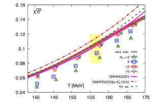
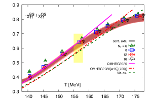
Figure 9: Comparison of HRG model calculations with QCD results for $\chi_{11}^{QS}$ (top) and the ratio $\chi_{11}^{BS}/\chi_{11}^{QS}$ (bottom). The dashed-dotted lines show results from a HRG model calculation where also the contribution of $K_{0}^{*}(700)$ is included in the list of hadron resonances. In the lower figure we show the result of an virial expansion for $\chi_{11}^{BS}$ taken from Fernández-Ramírez et al. (2018). The upper figure shows the result of a virial expansion, based on the analysis of S-wave scattering contributions in the $K$-$\pi$ channel to strangeness fluctuations Friman et al. (2015), as discussed in the text.

In Fig. 10 we compare results from QCD calculations to HRG model calculations that use lists of hadron resonances with (QMHRG) and without (PDGHRG) additional strange baryon resonances included. As can be seen the ratio $\mu_{S}/\mu_{B}$ obtained in QCD calculations when imposing the strangeness neutrality condition $n_{S}=0$ and $n_{Q}/n_{B}=0.4$ differs by about 15% from HRG model calculations, that only use the PDGHRG states, but is in good agreement with QMHRG model calculations. This shows that the ratio of strangeness and baryon chemical potentials indeed is sensitive to the spectrum of strange hadron resonances in a strongly interacting medium. We will discuss this further in a forthcoming publication, where we show that higher order contributions to $\mu_{S}/\mu_{B}$ are indeed negligible for $\mu_{B}/T\raise 1.29167pt\hbox{$<$\kern-7.5pt\raise-4.73611pt\hbox{$\sim$}}1$, which makes this ratio a good observable for probing thermal conditions in a strongly-interacting medium.

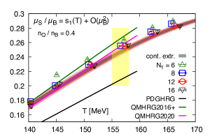
Figure 10: Leading order result for the ratio of strangeness and baryon chemical potentials versus temperature for the case $n_{Q}/n_{B}=0.4$. QCD results are compared to HRG model calculations using different spectra of hadronic resonances.

V.2 Volume dependence of the cumulant of net electric-charge fluctuations, $\chi_{2}^{Q}$

As can be seen in Fig. 2 (top, right) even at temperatures as low as $135$ MeV continuum extrapolated results for the second order cumulant of net electric-charge fluctuations still differ from HRG model calculations. At such low temperatures electric charge fluctuations are dominated by the contribution from pions. In this case it is well known that finite volume effects in a pion gas with mass $m_{\pi}\raise 1.29167pt\hbox{$<$\kern-7.5pt\raise-4.73611pt\hbox{$\sim$}}T$ can lead to significant deviations from results obtained in the thermodynamic limit Engels et al. (1982); Bhattacharyya et al. (2015); Karsch et al. (2016).

The lattice QCD calculations presented in Fig. 2 have been performed on lattices with a fixed ratio of spatial versus temporal extent, $N_{\sigma}/N_{\tau}=4$. I.e. the spatial extent of the physical volume, $L=N_{\sigma}a$, changes with temperature, $T=1/N_{\tau}a$, such that $LT=4$ stays constant. In the temperature range shown in Fig. 2, we have calculated $\chi_{2}^{Q}$ for a pion gas in a finite volume with $LT=4$. This can be done directly using the partition function of a Bose gas in a finite volume Bhattacharyya et al. (2015); Karsch et al. (2016). In order to mimic periodic boundary conditions and cubic box sizes as they are used in lattice QCD calculations, we instead used a scalar field theory discretized on a lattice as described in Engels et al. (1982). For a non-interacting pion and kaon gas we find that deviations from infinite volume results are well parametrized by a straight line ansatz in the temperature interval of interest, $T\in[130~{}{\rm MeV}:170~{}{\rm MeV}]$,

$$\frac{(\chi_{2}^{Q})_{LT=4}}{(\chi_{2}^{Q})_{LT=\infty}}=\begin{cases}0.997-0.126\ T/T_{pc,0}\;,\;{\rm pion}~{}{\rm gas}\\ 1.002-0.032\ T/T_{pc,0}\;,\;{\rm kaon}~{}{\rm gas}\end{cases}$$ (21)

	$\chi_{11}^{BQ}$	$\chi_{11}^{BS}$	$\chi_{11}^{QS}$	$(\chi_{2}^{Q})_{LT=4}$   [$\chi_{2}^{Q}$]	$\chi_{2}^{S}$	$\chi_{2}^{B}$	$\chi_{11}^{BS}/\chi_{2}^{S}$	$\chi_{11}^{BQ}/\chi_{2}^{B}$
QCD[this work]	0.0243(7)(9)	-0.066(4)(5)	0.106(3)(5)	0.413(8)(9)	0.279(9)(12)	0.115(5)(7)	-0.236(5)(6)	0.212(4)(5)
QMHRG2020[this work]	0.031(3)	-0.066(6)	0.103(5)	0.437(14) [0.466(15)]	0.272(14)	0.127(10)	-0.243(8)	0.244(3)
QMHRG2016+ Alba et al. (2017)	0.031(3)	-0.071(7)	0.104(5)	0.444(15) [0.472(15)]	0.277(16)	0.132(10)	-0.256(7)	0.235(2)
PDGHRG	0.030(2)	-0.046(4)	0.094(4)	0.419(12) [0.447(14)]	0.234(11)	0.106(8)	-0.197(6)	0.283(2)
EVHRG2020[$b=1~{}\rm{fm^{3}}$]	0.027(2)	-0.059(5)	0.103(5)	0.431(13) [0.459(15)]	0.264(13)	0.113(8)	-0.223(5)	0.243(2)
S-matrix[Friman et al. (2015),Fernández-Ramírez et al. (2018)]	0.020(1)	-0.062(5)	0.107(4)	–	–	–	–	–

Table 5: Continuum-extrapolated values of second order cumulants at $T_{pc,0}=156.5(1.5)$ MeV and for vanishing values of the chemical potentials. First error in QCD is obtained by linearly combining statistical and systematical error of our continuum extrapolations while the second one error reflects the error on the determination of $T_{pc,0}$. Similarly the error in the HRG is due to the error of $T_{pc,0}$. These results agree well with the continuum extrapolated data given in Bellwied et al. (2020). For $\chi_{2}^{Q}$ we give results calculated in a finite volume $LT\equiv N_{\sigma}/N_{\tau}=4$. Numbers in brackets give the corresponding infinite volume result.

At the pseudo-critical temperature, $T_{pc,0}$, the net electric-charge fluctuations in a pion gas in a volume $LT=4$ thus is about 12% smaller than in the infinite volume limit. In the HRG model, calculated with the resonance spectrum QMHRG2020, this distortion effect gets reduced by almost a factor two, reflecting the relative contribution of pions to the entire net electric-charge fluctuations. In the temperature interval $T\in[130~{}{\rm MeV}:180~{}{\rm MeV}]$ we find for a HRG model using the QMHRG2020 list of hadrons,

$$\frac{(\chi_{2}^{Q})_{LT=4}}{(\chi_{2}^{Q})_{LT=\infty}} = 1.324-1.290T/T_{pc,0}+1.316(T/T_{pc,0})^{2}$$ (22)

$$-0.411(T/T_{pc,0})^{3}\;,\;$$

This amounts to a 6% finite volume correction for $\chi_{2}^{Q}$ at the pseudo-critical temperature, $T_{pc,0}$, which only changes slowly as function of temperature. We show this finite volume correction to the QMHRG2020 result for $\chi_{2}^{Q}$ in Fig. 2 (top, right).

Using the finite volume corrected QMHRG2020 results for a comparison with QCD results in a finite volume, we find that at $T_{pc,0}$ the latter are still smaller by about 5%. this is consistent with large deviations observed in the charged baryon sector ($\chi_{11}^{BQ}$) which contributes only about 15% to the total electric charge fluctuations.

V.3 Comparison of QCD results with various model calculations at $T_{pc,0}$

Continuum extrapolated lattice QCD results for all six second order cumulants at $T_{pc,0}$ and corresponding results from HRG model calculations, using different hadronic resonance spectra, as well as results from S-matrix calculations are summarized in Table 5. Here we also give results for two of the three independent ratios of second order cumulants. The third ratio would involve $\chi_{2}^{Q}$, for which at present no infinite volume extrapolated result exists.

VI Conclusions

We have presented an update of continuum extrapolated results for second order cumulants of conserved charge fluctuations and their cross-correlations. These results are based on high-statistics data obtained in simulations within the HISQ discretization scheme for staggered fermions. Our results are found to be consistent with previous results obtained by using the stout discretization scheme for staggered fermions Bellwied et al. (2020).

We compiled a new list of hadron resonances, QMHRG2020, which differs from QMHRG2016+ in particular in the strange baryon sector. HRG model calculations with QHMHRG2020 provide a good description of strangeness fluctuations and correlations with baryon-number and electric charge fluctuations, respectively. Deviations are found to be less than 10% in the temperature range $135~{}{\rm MeV}<T<T_{pc,0}$. This puts stringent bounds on the magnitude of excluded volume parameters for strange baryon interactions in EVHRG models.

The largest differences between QCD results and HRG model calculations have been found for correlations between net baryon-number and electric charge fluctuations. They amount to more than 20% at $T_{pc,0}$ when comparing QCD with HRG models based on point-like, non-interacting resonances. Modeling these deviations, and in particular the quite different temperature dependence of $\chi_{11}^{BQ}$ found in the vicinity of $T_{pc,0}$, in excluded volume HRG models would require a large excluded volume parameter $b>1$ fm³.

Calculations based on a virial expansion capture basic features of the interplay between repulsive and attractive interactions in the strongly interacting hadronic medium. They successfully explain why in particular the strange meson resonance $K_{0}^{*}(700)$ does not contribute in that medium. They also qualitatively describe the smaller magnitude of $\chi_{11}^{BQ}$ found in QCD compared to HRG model calculations with point-like, non-interacting resonances. However, in order to achieve quantitative agreement with QCD modeling of interactions that are not captured in calculations of the second virial coefficient is needed.

The results presented here form the basis for a systematic analysis of second order cumulants at non-vanishing values of the chemical potentials. This will be discussed in a forthcoming publication. All data from our calculations, presented in the figures of this paper, can be found in Bollweg et al. (2021).

Acknowledgments.— This work was supported by: (i) The U.S. Department of Energy, Office of Science, Office of Nuclear Physics through the Contract No. DE-SC0012704; (ii) The U.S. Department of Energy, Office of Science, Office of Nuclear Physics and Office of Advanced Scientific Computing Research within the framework of Scientific Discovery through Advance Computing (SciDAC) award Computing the Properties of Matter with Leadership Computing Resources; (iii) The Deutsche Forschungsgemeinschaft (DFG, German Research Foundation) - Project number 315477589-TRR 211; (iv) The grant 05P2018 (ErUM-FSP T01) of the German Bundesministerium für Bildung und Forschung; (v) The grant 283286 of the European Union.

This research used awards of computer time provided by: (i) The INCITE program at Oak Ridge Leadership Computing Facility, a DOE Office of Science User Facility operated under Contract No. DE-AC05-00OR22725; (ii) The ALCC program at National Energy Research Scientific Computing Center, a U.S. Department of Energy Office of Science User Facility operated under Contract No. DE-AC02-05CH11231; (iii) The INCITE program at Argonne Leadership Computing Facility, a U.S. Department of Energy Office of Science User Facility operated under Contract No. DE-AC02-06CH11357; (iv) The USQCD resources at the Thomas Jefferson National Accelerator Facility.

This research also used computing resources made available through: (i) a PRACE grant at CINECA, Italy; (ii) the Gauss Center at NIC-Jülich, Germany; (iii) the GPU-cluster at Bielefeld University, Germany.

Appendix A Parametrization of $a/r_{1}$ and $af_{K}$

In order to estimate systematic errors in our continuum extrapolations we used two observables to set the scale for the lattice spacing at finite values of the gauge coupling $\beta\equiv 10/g^{2}$. We use the length scale $r_{1}$ which is deduced from the short distance part of the heavy quark potential and the kaon decay constant, which is obtained from fits to the long distance behavior of strange meson correlation functions. Both parametrizations have already been introduced and used by us in Bazavov et al. (2014a).

Using the two-loop beta-function of 3-flavor QCD,

$$f(\beta)=\left(\frac{10b_{0}}{\beta}\right)^{-b_{1}/(2b_{0}^{2})}\exp(-\beta/(20b_{0}))$$

with $b_{0}=9/(16\pi^{2})$ and $b_{1}=1/(4\pi^{4})$ we parametrize $a/r_{1}$ and $af_{K}$ as

$$a/r_{1}(\beta) = \frac{c_{0}f(\beta)+c_{2}(10/\beta)f^{3}(\beta)}{1+d_{2}(10/\beta)f^{2}(\beta)}\;,$$ (23)

$$af_{K}(\beta) = \frac{c_{0}^{K}f(\beta)+c_{2}^{K}(10/\beta)f^{3}(\beta)}{1+d_{2}^{K}(10/\beta)f^{2}(\beta)}\;.$$ (24)

For $a/r_{1}$ we use

$$c_{0}=43.16(15)\; c_{2}=339472(21144)\;\;,$$ , (25)

$$d_{2}=5452(387)\;.$$

This parametrization is consistent with that given in Bazavov et al. (2014a). The parameters changed slightly which reflects our new bootstrap analysis of the data for $a/r_{1}$. For $af_{K}$ we use

$$c_{0}^{K}=7.486(25)\; c_{2}^{K}=41935(2247)\;\;,$$ , (26)

$$d_{2}^{K}=3273(224)\;.$$

This parametrization takes into account systematic errors on the determination of the $af_{K}$ scale at non-zero values of the lattices spacing, which arise from the fact that the original data taken for $af_{K}$ are not directly taken on the LCP and needed to be corrected as discussed in appendix C.3 of Bazavov et al. (2014a). In the continuum limit our parametrization gives for the relation of $r_{1}$ and $f_{K}$ in the continuum limit,

$$r_{1}f_{K}=\frac{c_{0}^{K}}{c_{0}}=0.1734(9)\;,$$ (27)

which for $r_{1}=0.3106$ fm gives for the kaon decay constant the FLAG average value $f_{K}=155.7/\sqrt{2}$ MeV Aoki et al. (2020). This value is used in all our figures when showing temperature scales in physical units.

For our spline interpolations at non-zero lattice spacing, i.e. at fixed temporal lattice extent $N_{\tau}$ we add to the statistical error of our data, determined at a certain value of the coupling $\beta$, a systematic error arising from the width of the bootstrap band at this $\beta$-value. This is used as an error on the $T$-scale (x-axis) when performing spline interpolations of our data at fixed $N_{\tau}$.

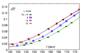
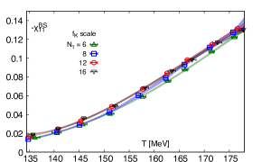
Figure 11: Spline interpolations for the cumulant $\chi_{11}^{BS}$ performed with the temperature scales obtained from $r_{1}$ (top) and $f_{K}$ (bottom) for $N_{\tau}=6,\ 8,\ 12,\ 16$.

Appendix B Fits to second order cumulants

Using the temperature scales given in Appendix A we performed spline interpolations of our data for each value of $N_{\tau}$. These interpolations have been done using 800 bootstrap samples on each of the four different lattice sizes. These interpolations are shown in Fig.11 for the case of $\chi_{11}^{BS}$ using $a/r_{1}$ (left) and $af_{K}$ (right). Errors on the spline interpolation are obtained from a bootstrap analysis where each data point has its statistical error and a systematic error arising from the errors on $a/r_{1}$ and $af_{K}$, respectively. Continuum extrapolations at fixed temperature are then performed using data at each $N_{\tau}$ value with errors given by the error band of the spline interpolations. We performed fits linear and quadratic in $1/N_{\tau}^{2}$, as introduced in Eq. 13 and Eq. 14, respectively. has been changed to Fits to $\chi_{11}^{BS}$, $\chi_{11}^{BQ}$, $\chi_{11}^{QS}$ and $\chi_{2}^{Q}$ performed at some temperature values, are shown in Fig. 12.

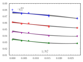
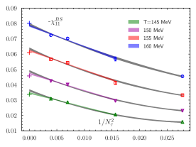
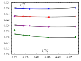
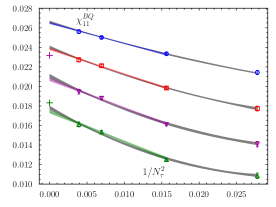
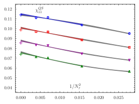
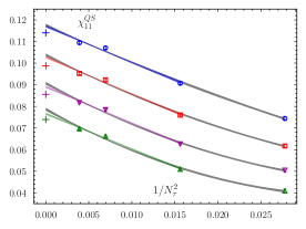
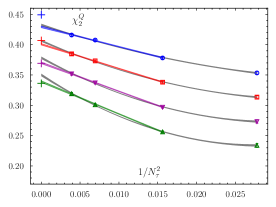
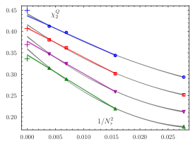
Figure 12: Continuum extrapolations for the cumulants $\chi_{11}^{BS}$, $\chi_{11}^{BQ}$, $\chi_{11}^{QS}$ and $\chi_{2}^{Q}$ (top to bottom) performed with the temperature scales obtained from $f_{K}$ (left) and $r_{1}$ (right) using linear and quadratic extrapolations in $1/N_{\tau}^{2}$. Shown are results for four values of the temperature below and close to the pseudo-critical temperature of $(2+1)$-flavor QCD. Also shown are results obtained in HRG model calculations using the QMHRG2020 list of hadrons (crosses). Note that for $\chi_{11}^{BQ}$ and $\chi_{2}^{Q}$ these HRG results are not shown for all temperature values as the deviations from the corresponding QCD results are too large. For $\chi_{2}^{Q}$ QMHRG2020 with the finite-volume corrected contributions for pions and kaons in a volume $LT\equiv N_{\sigma}/N_{\tau}=4$ has been used.

In the case of quadratic fits we have used the data sets for all $N_{\tau}$ and for linear extrapolations only results for $N_{\tau}>6$ have been used. As can be seen the quadratic fits generally have larger statistical errors and a $\chi^{2}/dof$ which is (5-10) times larger. Linear extrapolations for the $N=\tau=8,\ 12,\ 16$ data sets generally yield $\chi^{2}/dof\simeq 1$. This also is the case for the electric charge fluctuations, $\chi_{2}^{Q}$, except for the two lowest temperatures, $T=135$ MeV and $140$ MeV, where the $\chi^{2}/dof$ is about 2, but becomes even larger when using quadratic fits that include the $N_{\tau}=6$ data sets. We thus used results from the linear extrapolations in our final analysis.

Appendix C Comparison of QMHRG2020 and QMHRG2016+

We list here eight strange baryon resonances that are treated differently in QMHRG2020 and QMHRG2016+ lists of hadrons. When eliminating these states from the QMHRG2016+ list HRG model calculations performed with the reduced QMHRG2016+ list agree with those performed with the QMHRG2020, although some values of the masses differ slightly as QMHRG2020 is based on the masses given in Ref. Faustov and Galkin (2015), while QMHRG2016+ use masses from Ref. Capstick and Isgur (1986).

Particle	PDG [MeV]	Quark Model [MeV]
	Zyla et al. (2020)	Capstick and Isgur (1986)      Faustov and Galkin (2015)
$\Lambda$(1405)	1405	1550    1406
$\Lambda$(1830)	1830	1775    1861
$\Lambda$(2050)	2050	2035    2030
$\Lambda$(2325)	2325	2185    2322
$\Sigma$(1750)	1750	1695    1747
$\Sigma$(1910)	1910	1755    1856
(was $\Sigma$(1940))
$\Sigma$(1940)	1940	2010    2025
$\Sigma$(2070)	2070	2030    2062

Table 6: Strange baryon resonances that are treated differently in the QMHRG2020 and QMHRG2016+ lists. While only states listed by the PDG Zyla et al. (2020) are kept in the former, also the corresponding quark model states are kept in the latter.

References

- Bazavov et al. (2019a) A. Bazavov et al. (HotQCD), Phys. Lett. B 795, 15 (2019a), arXiv:1812.08235 [hep-lat] .
- Borsanyi et al. (2020) S. Borsanyi, Z. Fodor, J. N. Guenther, R. Kara, S. D. Katz, P. Parotto, A. Pasztor, C. Ratti, and K. K. Szabo, Phys. Rev. Lett. 125, 052001 (2020), arXiv:2002.02821 [hep-lat] .
- Bonati et al. (2015) C. Bonati, M. D’Elia, M. Mariti, M. Mesiti, F. Negro, and F. Sanfilippo, Phys. Rev. D92, 054503 (2015), arXiv:1507.03571 [hep-lat] .
- (4) P. Braun-Munzinger, K. Redlich, and J. Stachel, Quark Gluon Plasma 3, 491 (2003), 10.1142/9789812795533-0008, arXiv:nucl-th/0304013 .
- Hagedorn (1965) R. Hagedorn, Nuovo Cim. Suppl. 3, 147 (1965).
- Karsch and Redlich (2011) F. Karsch and K. Redlich, Phys. Lett. B 695, 136 (2011), arXiv:1007.2581 [hep-ph] .
- Andronic et al. (2018) A. Andronic, P. Braun-Munzinger, K. Redlich, and J. Stachel, Nature 561, 321 (2018), arXiv:1710.09425 [nucl-th] .
- Dashen et al. (1969) R. Dashen, S.-K. Ma, and H. J. Bernstein, Phys. Rev. 187, 345 (1969).
- Venugopalan and Prakash (1992) R. Venugopalan and M. Prakash, Nucl. Phys. A 546, 718 (1992).
- Lo et al. (2013) P. M. Lo, B. Friman, O. Kaczmarek, K. Redlich, and C. Sasaki, Phys. Rev. D 88, 014506 (2013).
- Fernández-Ramírez et al. (2018) C. Fernández-Ramírez, P. M. Lo, and P. Petreczky, Phys. Rev. C 98, 044910 (2018), arXiv:1806.02177 [hep-ph] .
- Andronic et al. (2019) A. Andronic, P. Braun-Munzinger, B. Friman, P. M. Lo, K. Redlich, and J. Stachel, Phys. Lett. B 792, 304 (2019), arXiv:1808.03102 [hep-ph] .
- Hagedorn and Rafelski (1980a) R. Hagedorn and J. Rafelski, Phys. Lett. B 97, 136 (1980a), CERN-TH-2922 .
- Hagedorn and Rafelski (1980b) R. Hagedorn and J. Rafelski, in International Conference on Nuclear Physics (1980) CERN-TH-2947, C80-08-24-1 .
- Gorenstein et al. (1981) M. I. Gorenstein, V. K. Petrov, and G. M. Zinovev, Phys. Lett. B 106, 327 (1981).
- Vovchenko et al. (2017a) V. Vovchenko, M. I. Gorenstein, and H. Stoecker, Phys. Rev. Lett. 118, 182301 (2017a), arXiv:1609.03975 [hep-ph] .
- Vovchenko et al. (2017b) V. Vovchenko, A. Pasztor, Z. Fodor, S. D. Katz, and H. Stoecker, Phys. Lett. B 775, 71 (2017b), arXiv:1708.02852 [hep-ph] .
- Taradiy et al. (2019) K. Taradiy, A. Motornenko, V. Vovchenko, M. I. Gorenstein, and H. Stoecker, Phys. Rev. C 100, 065202 (2019), arXiv:1904.08259 [hep-ph] .
- Olive (1981) K. A. Olive, Nucl. Phys. B 190, 483 (1981).
- Olive (1982) K. A. Olive, Nucl. Phys. B 198, 461 (1982).
- Huovinen and Petreczky (2018) P. Huovinen and P. Petreczky, Phys. Lett. B 777, 125 (2018), arXiv:1708.00879 [hep-ph] .
- Goswami et al. (2021a) J. Goswami, F. Karsch, C. Schmidt, S. Mukherjee, and P. Petreczky, Acta Phys. Polon. Supp. 14, 251 (2021a), arXiv:2011.02812 [hep-lat] .
- Goswami et al. (2021b) J. Goswami, F. Karsch, S. Mukherjee, P. Petreczky, and C. Schmidt, (2021b), arXiv:2109.00268 [hep-lat] .
- Karthein et al. (2021) J. M. Karthein, V. Koch, C. Ratti, and V. Vovchenko, (2021), arXiv:2107.00588 [nucl-th] .
- Follana et al. (2007) E. Follana, Q. Mason, C. Davies, K. Hornbostel, G. Lepage, J. Shigemitsu, H. Trottier, and K. Wong (HPQCD, UKQCD), Phys. Rev. D 75, 054502 (2007), arXiv:hep-lat/0610092 .
- Bazavov et al. (2020) A. Bazavov et al., Phys. Rev. D 101, 074502 (2020), arXiv:2001.08530 [hep-lat] .
- Bazavov et al. (2017a) A. Bazavov et al., Phys. Rev. D 95, 054504 (2017a), arXiv:1701.04325 [hep-lat] .
- Bazavov et al. (2014a) A. Bazavov et al. (HotQCD), Phys. Rev. D 90, 094503 (2014a), arXiv:1407.6387 [hep-lat] .
- Bazavov et al. (2019b) A. Bazavov et al., Phys. Rev. D 100, 094510 (2019b), arXiv:1908.09552 [hep-lat] .
- Bazavov et al. (2012a) A. Bazavov et al., Phys. Rev. Lett. 109, 192302 (2012a), arXiv:1208.1220 [hep-lat] .
- Bazavov et al. (2012b) A. Bazavov et al. (HotQCD), Phys. Rev. D 86, 034509 (2012b), arXiv:1203.0784 [hep-lat] .
- Bellwied et al. (2020) R. Bellwied, S. Borsanyi, Z. Fodor, J. N. Guenther, J. Noronha-Hostler, P. Parotto, A. Pasztor, C. Ratti, and J. M. Stafford, Phys. Rev. D 101, 034506 (2020), arXiv:1910.14592 [hep-lat] .
- Zyla et al. (2020) P. Zyla et al. (Particle Data Group), PTEP 2020, 083C01 (2020).
- Capstick and Isgur (1986) S. Capstick and N. Isgur, Phys. Rev. D 34, 2809 (1986).
- Ebert et al. (2009) D. Ebert, R. Faustov, and V. Galkin, Phys. Rev. D 79, 114029 (2009), arXiv:0903.5183 [hep-ph] .
- Faustov and Galkin (2015) R. Faustov and V. Galkin, Phys. Rev. D 92, 054005 (2015), arXiv:1507.04530 [hep-ph] .
- Edwards et al. (2011) R. G. Edwards, J. J. Dudek, D. G. Richards, and S. J. Wallace, Phys. Rev. D 84, 074508 (2011), arXiv:1104.5152 [hep-ph] .
- Edwards (2020) R. G. Edwards, PoS LATTICE2019, 253 (2020).
- Allton et al. (2005) C. R. Allton, M. Doring, S. Ejiri, S. J. Hands, O. Kaczmarek, F. Karsch, E. Laermann, and K. Redlich, Phys. Rev. D 71, 054508 (2005), arXiv:hep-lat/0501030 .
- Bazavov et al. (2017b) A. Bazavov et al. (HotQCD), Phys. Rev. D 96, 074510 (2017b), arXiv:1708.04897 [hep-lat] .
- Bazavov et al. (2010) A. Bazavov et al. (MILC), PoS LATTICE2010, 074 (2010), arXiv:1012.0868 [hep-lat] .
- Aoki et al. (2020) S. Aoki et al. (Flavour Lattice Averaging Group), Eur. Phys. J. C 80, 113 (2020), arXiv:1902.08191 [hep-lat] .
- Bazavov et al. (2014b) A. Bazavov et al., Phys. Rev. Lett. 113, 072001 (2014b), arXiv:1404.6511 [hep-lat] .
- Menapara and Rai (2021) C. Menapara and A. K. Rai, Chin. Phys. C 45, 063108 (2021), arXiv:2104.00439 [hep-ph] .
- Fiore et al. (1977) R. Fiore, R. Page, and L. Sertorio, Nuovo Cim. A 37, 45 (1977).
- Broniowski et al. (2015) W. Broniowski, F. Giacosa, and V. Begun, Phys. Rev. C 92, 034905 (2015), arXiv:1506.01260 [nucl-th] .
- Friman et al. (2015) B. Friman, P. M. Lo, M. Marczenko, K. Redlich, and C. Sasaki, Phys. Rev. D 92, 074003 (2015), arXiv:1507.04183 [hep-ph] .
- Bollweg et al. (2021) D. Bollweg, J. Goswami, O. Kaczmarek, F. Karsch, S. Mukherjee, P. Petreczky, C. Schmidt, and P. Scior, (2021), https://doi.org/10.4119/unibi/2957724.
- Alba et al. (2017) P. Alba et al., Phys. Rev. D 96, 034517 (2017), arXiv:1702.01113 [hep-lat] .
- Lo et al. (2018) P. M. Lo, B. Friman, K. Redlich, and C. Sasaki, Phys. Lett. B 778, 454 (2018), arXiv:1710.02711 [hep-ph] .
- Lo et al. (2017) P. M. Lo, B. Friman, M. Marczenko, K. Redlich, and C. Sasaki, Phys. Rev. C 96, 015207 (2017), arXiv:1703.00306 [nucl-th] .
- Capstick and Roberts (1994) S. Capstick and W. Roberts, Phys. Rev. D 49, 4570 (1994), arXiv:nucl-th/9310030 .
- Hunt and Manley (2019) B. C. Hunt and D. M. Manley, Phys. Rev. C 99, 055205 (2019), arXiv:1810.13086 [nucl-ex] .
- Ablikim et al. (2006) M. Ablikim et al. (BES), Phys. Lett. B 633, 681 (2006), arXiv:hep-ex/0506055 .
- Ablikim et al. (2011) M. Ablikim et al. (BES), Phys. Lett. B 698, 183 (2011), arXiv:1008.4489 [hep-ex] .
- Giacosa (2019) F. Giacosa, Acta Phys. Pol. B Proc. Suppl. 12, 283 (2019), arXiv:1811.00298 [hep-ph] .
- Engels et al. (1982) J. Engels, F. Karsch, and H. Satz, Nucl. Phys. B 205, 239 (1982).
- Bhattacharyya et al. (2015) A. Bhattacharyya, R. Ray, S. Samanta, and S. Sur, Phys. Rev. C 91, 041901 (2015), arXiv:1502.00889 [hep-ph] .
- Karsch et al. (2016) F. Karsch, K. Morita, and K. Redlich, Phys. Rev. C 93, 034907 (2016), arXiv:1508.02614 [hep-ph] .