Registration of 3D Point Sets Using Correntropy Similarity Matrix

Abstract

This work focuses on Registration or Alignment of 3D point sets. Although the Registration problem is a well established problem and it’s solved using multiple variants of Iterative Closest Point (ICP) Algorithm, most of the approaches in the current state of the art still suffers from misalignment when the Source and the Target point sets are separated by large rotations and translation. In this work, we propose a variant of the Standard ICP algorithm, where we introduce a Correntropy Relationship Matrix in the computation of rotation and translation component which attempts to solve the large rotation and translation problem between Source and Target point sets. This matrix is created through correntropy criterion which is updated in every iteration. The correntropy criterion defined in this approach maintains the relationship between the points in the Source dataset and the Target dataset. Through our experiments and validation we verify that our approach has performed well under various rotation and translation in comparison to the other well-known state of the art methods available in the Point Cloud Library (PCL) as well as other methods available as open source. We have uploaded our code in the github repository for the readers to validate and verify our approach https://github.com/aralab-unr/CoSM-ICP.

1 Introduction

Registering two point clouds is an active area of research in the community. Registration is the process of aligning two point cloud datasets of the same scene, which are separated by a certain transformation (rotation and translation). The problem of registration can be explained as finding the transformation between two point clouds such that the relative error between the 2 point sets is minimized. The problem of registration is a significant component in Simultaneous Localization and Mapping (SLAM) for robotics and other visual data matching algorithms [1]. The relative transformation computed from point clouds acquired at close time intervals from a 3D sensor can be used to compute the overall trajectory of a system [2, 1].

Early approaches for 3D point cloud registration can be attributed to Besl and MacKay [3, 4] and Arun et.al [3], which consists of computing the centroid for both Source and Target datasets. Each point from both the datasets is subtracted from their respective centroids and later on, Singular Value Decomposition (SVD) is used to compute the rotation component. This procedure is performed iteratively until the relative mean square error between the point cloud datasets is minimized, and hence it is termed as Iterative Closest Point (ICP) Algorithm. Since then variants of ICP have been introduced, a point-to-plane variant of ICP operates on taking advantage of surface normal information [5]. Instead of minimizing the root mean square of the individual points as done in the generalized version of the ICP, the point to plane algorithm minimizes error along the surface normal [6, 7, 8, 9, 10, 11, 12].

Despite the various advances in the registration methodologies, handling the situation where the data set is noisy is still a major concern. If the noise is Gaussian, we can remove most of it from the data. However, when the noise is non-Gaussian (e.g., shot noises), it becomes difficult to resolve. Hence, it is important to address the problem of handling non-Gaussian noise. The idea of Correntropy has seen widespread use in modern machine learning, signal processing, and other related fields [13, 14]. Correntropy is a measure of similarity between two random variables and has been implemented with the traditional Kalman filter [15]. Some recent work [14, 16, 17, 18, 19] has introduced the Correntropy concept to the registration problem to overcome the drawbacks of the ICP algorithm. In the traditional ICP algorithm, if any of the point cloud dataset (Source or Target) is affected by non-Gaussian noise, the ICP fails drastically and affects the overall transformation estimation of the point clouds. In this work, we show through basic examples on how the addition of non-Gaussian noise can affect the traditional ICP as well as compare how our approach can be better than the traditional ICP algorithm and it’s variants. We also compare our approach with the well known Normal Distribution Transform (NDT) algorithm available in the PCL library.

In this work, we propose a Correntropy Similarity Matrix Iterative Closest Point (CoSM ICP) algorithm. In our approach, we introduce a matrix of size $N\times N$ which maintains a ‘numeric’ relationship between Source and Target dataset points (size of Source dataset and Target dataset is $N$, hence the matrix size is $N\times N$). This numeric relationship is calculated through the well-known correntropy criterion, and it is updated at every iteration. It is calculated only between the nearest points from Source dataset to the Target dataset, thereby making the Similarity Matrix a sparse matrix. Our approach not only provides a significant improvement in the alignment of Source and Target dataset under various rotations and translations, it also proves quite effective against non-Gaussian outliers affecting the dataset. In addition to evaluating our approach in multiple datasets, we also evaluate the method where we inject the Source dataset with random false values and through experimental comparison with the traditional ICP and other approaches, we evaluate how well our approach can estimate the transformation between the ’infected’ Source and the Target dataset and we see how our approach performs better than the well known state of the art methods. Along side estimating accurate transformations, handling shot-noise or the non-Gaussian noise vectors is a critical component for better transformation estimation and is the driving force for our work.

Inspired by this Correntropy concept, we fuse it with the ICP algorithm, called Correntropy Similarity Matrix ICP or CoSM-ICP. Our main contribution to this work can be summarized as follows:

• We propose a new data registration algorithm in which the Correntropy Similarity Matrix ICP is introduced.

• We evaluate our approach on various randomly generated transformation matrices between Source and the Target.

• Through evaluation on these random transformation matrices we see how well our approach performs better than the other well known state of the art methods.

• We also introduce outliers in the Source dataset and evaluate our approach on the ’infected’ Source dataset.

• We compare our approach with other approaches on the ’infected’ Source dataset and see through results how well our approach performs better.

The remaining paper is organized as follows: Section 2 introduces the idea of Correntropy and its underlying concepts. Section 3 describes our proposed method and it’s implementation. The results and evaluation of our proposed method are discussed in Section 4. Conclusions and future work discussion are given in Section V.

2 Correntropy Criterion

Table 1: Nomenclature

Variables	Usages
$\mathbb{{P}_{s}}$	Source Point Cloud Set.
$\mathbb{{P}_{t}}$	Target Point Cloud Set.
$N$	Total number of points in point clouds $\mathbb{{P}_{s}}$ and $\mathbb{{P}_{t}}$.
$j,k$	Index of every point in point cloud where $j,k=1,..,N$.
$\mathbb{p}_{j}$	Individual 3D point $(x_{j},y_{j},z_{j})$ in a point cloud $\mathbb{{P}_{s}}$, or $\mathbb{p}_{j}\in\mathbb{P}_{s}$.
$\mathbb{q}_{k}$	Individual 3D point $(x_{k},y_{k},z_{k})$ in a point cloud $\mathbb{{P}_{t}}$, or $\mathbb{q}_{k}\in\mathbb{P}_{t}$.
$G_{\sigma}$	Gaussian kernel function with bandwidth $\sigma$.
$\mathbb{R}$	Rotation matrix.
$\mathbb{tr}$	Translation vector.
$\varepsilon^{2}$	Root mean square error.
$s$	Scaling factor.
SM	Similarity Matrix.
$\mathbb{s_{cen}}$,$\mathbb{t_{cen}}$	Centroids computation of Source and Target datasets.

We begin by describing the mathematical representation of point cloud data and develop our algorithm based on it. We denote Source point cloud as $\mathbb{{P}_{s}}$ and Target point cloud as $\mathbb{{P}_{t}}$. The points in the point cloud $\mathbb{{P}_{s}}$ contains $N$ points in which each point can be referenced as $\mathbb{p}_{j}=\left\{x_{j},y_{j},z_{j}\right\}$, where $x_{j},y_{j},z_{j}$ denotes the 3D coordinates of the point $\mathbb{p}_{j}$. Similarly, the points in the point cloud $\mathbb{{P}_{t}}$ contains $N$ points in which each point can be represented as $\mathbb{q}_{k}=\left\{x_{k},y_{k},z_{k}\right\}$, where $x_{k},y_{k},z_{k}$ denotes the 3D coordinates of the point $\mathbb{q}_{k}$. Throughout the paper, we describe a matrix as bold and capitalized letters, a vector is represented as bold and lowercase letters and the rest of the variables (single dimension) are represented as lowercase variables. Figure 1 shows a brief description of the point clouds and Table 1 denotes the mathematical notations used throughout this work.

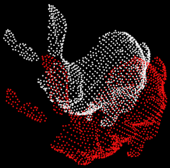
(a)

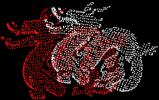
(b)

Figure 1: (a) Red is the Source point cloud $\mathbb{{P}_{s}}$ (bunny rabbit). $\mathbb{{P}_{s}}$ contains $N$ points $\mathbb{p}_{j}$ ($j=1,..,N$), each of which is a 3D representation $x_{j},y_{j},z_{j}$. White is the Target point cloud $\mathbb{{P}_{t}}$. $\mathbb{{P}_{t}}$ contains $N$ points $\mathbb{q_{k}}$ ($k=1,..,N$), each of which is a 3D representation $x_{k},y_{k},z_{k}$. Same goes for the dragon dataset in (b).

We use the Correntropy concept between the Source point cloud and the Target point cloud. Correntropy has proved beneficial to remove large outliers [13]. Correntropy is essentially a similarity measure of two random variables. We use the Correntropy concept between Source and Target point clouds. In this scenario, we are measuring the similarity between points $\mathbb{p}_{j}$ and $\mathbb{q}_{k}$ from the point clouds $\mathbb{{P}_{s}}$ and $\mathbb{{P}_{t}}$, respectively. Then the Correntropy criterion between points $\mathbb{p}_{j}$ and $\mathbb{q}_{k}$ can be mathematically represented as :

$$\mathbb{\textit{V}_{\sigma}}(\mathbb{p}_{j},\mathbb{q}_{k})=\mathbb{\textit{E}}[\kappa_{\sigma}(\mathbb{p}_{j}-\mathbb{q}_{k})].$$ (1)

Equ. (1) also refers to in common literature as a cross-Correntropy of two random variables [20, 21, 15]. In Equ. (1), E[.] refers to the expectation of the variable, and $\kappa_{\sigma}$ denotes the kernel function. We can manually choose the size of the kernel function (also referred to as bandwidth $\sigma$). In our approach, we use the Gaussian kernel function where we redefine the Correntropy function as:

$$\mathbb{\textit{V}_{\sigma}}(\mathbb{p}_{j},\mathbb{q}_{k})=\frac{1}{N}\sum_{j,k=1}^{N}\mathbb{\textit{G}_{\sigma}}(\mathbb{p}_{j}-\mathbb{q}_{k}).$$ (2)

From Equ.(2),

$$G_{\sigma}(\mathbb{p}_{j}-\mathbb{q}_{k})=exp(-\frac{\left\|\mathbb{p}_{j}-\mathbb{q}_{k}\right\|^{2}}{2\sigma^{2}}),$$ (3)

where $\sigma$ is the bandwidth or the kernel size of the Gaussian kernel. From Equ. (3) it becomes evident that if $\mathbb{p}_{j}=\mathbb{q}_{k}$ Gaussian Correntropy is maximum, and the Gaussian Correntropy function is positive and bounded [20, 21, 15].

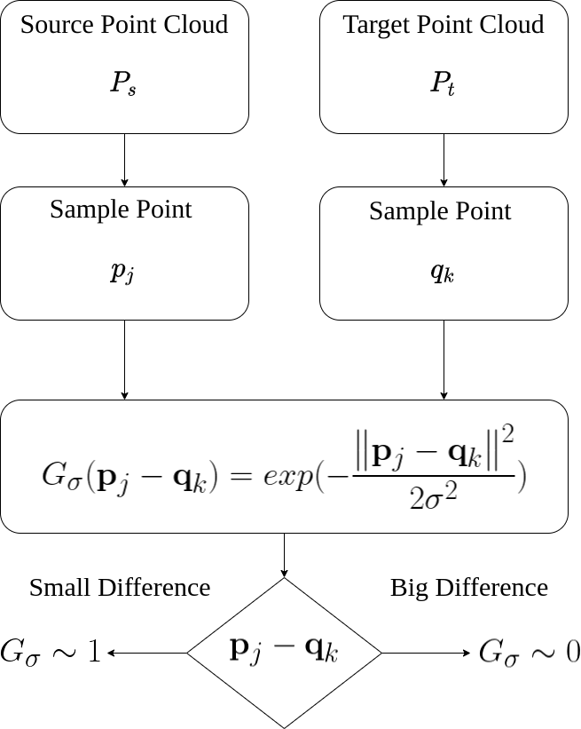
Figure 2: Correntropy Criterion. Here, when the difference between the points ($\mathbb{p}_{j}-\mathbb{q}_{k}$) is small, i..e., when they are similar, and the Gaussian kernel function $G_{\sigma}$ approaches to 1. On the contrary, when the difference is large, the Gaussian kernel function approaches to 0.

Fig. 2 shows the basic understanding of the Correntropy criterion. We see that when the difference between the points ($\mathbb{p}_{j}-\mathbb{q}_{k}$) is small, i.e., they are similar, and the Gaussian kernel function $G_{\sigma}$ approaches to 1. On the contrary, when the difference is large, the Gaussian kernel function approaches 0. This essentially means that when a potentially changed data point (for e.g., $\mathbb{q}_{k}$ ), is far varied from $\mathbb{p}_{j}$, the Gaussian kernel signifies that the points $\mathbb{p}_{j}$ and $\mathbb{q}_{k}$ are not similar. Intuitively, this similarity is dependent on the value of $\sigma$. This technique allows us to reject the faulty data point (shot noise or non-Gaussian noise) $\mathbb{q}_{k}$. This idea of calculating the maximum similarity as given in Equ. (3) is called the maximum Correntropy criterion.

When the value of $\mathbb{q}_{k}$ approaches $\infty$ then the kernel function approaches 0, i.e.,

$$\lim_{\mathbb{q}_{k}\to\infty}G_{\sigma}=0.$$ (4)

Intuitively, when the Gaussian Kernel shrinks to $0$, the Correntropy approaches the value $p(\mathbb{p}_{j}=\mathbb{q}_{k})$ [22].

3 Proposed Method

3.1 Correntropy Similarity Matrix with Iterative Closest Point Algorithm

Given the general description of the Correntropy concept in the previous section, we extend this idea of Correntropy to the well known ICP algorithm. Traditional ICP  [3] describes the alignment of point clouds such that the Mean Square Error (MSE) between point sets is minimized. The MSE is the key criterion of convergence in ICP and its variants. ICP revolves around the problem of aligning points sets $\mathbb{{P}_{s}}$ and $\mathbb{{P}_{t}}$. We denote the point sets as $\mathbb{P}_{s}=\left\{[\mathbb{p}_{j}]_{j=1}^{N}\right\}$ (here $\left\{\right\}$ denotes a point set) and $\mathbb{P}_{t}=\left\{[\mathbb{q}_{k}]_{k=1}^{N}\right\}$, respectively. Our goal is to best align Source point set $\mathbb{{P}_{s}}$ to Target point set (or a model point set) $\mathbb{{P}_{t}}$. This leads to finding the appropriate rotation and translation between the two point sets, which essentially means how much units the Source dataset needs to be translated ($\mathbb{tr}$) and rotated ($\mathbb{R}$) such that Source point set $\mathbb{{P}_{s}}$ is best aligned with $\mathbb{{P}_{t}}$ given that it satisfies a particular criterion (Root Mean Square Error (RMSE) threshold). This process is commonly known as registration between the Source $\mathbb{{P}_{s}}$ and the Target $\mathbb{{P}_{t}}$ is defined as finding the translation $\mathbb{tr}$ and the rotation $\mathbb{R}$ component such that $\mathbb{{P}_{s}}$ is in best alignment with $\mathbb{{P}_{t}}$.

Now, the problem can be written as: find the best $\mathbb{R}$ and $\mathbb{tr}$ such that the MSE, $\varepsilon^{2}$, between 2 point clouds is minimized. This problem can be mathematically written as,

$$\varepsilon^{2}=\sum_{j,k=1}^{N}\left\|\mathbb{p}_{j}-(s\mathbb{R}\mathbb{q}_{k}+\mathbb{tr})\right\|^{2},$$ (5)

where $s$ is the scaling component. $\mathbb{p}_{j}\in\mathbb{{P}_{s}}$ is the set of all the points in the Source point set, and $\mathbb{q}_{k}\in\mathbb{P}_{t}$ is the set of all the points in the Target point set ($j,k=1,...,N$).

Our work is built on the work of Arun et al.[3] and it is well known from their work that initially we compute the corresponding points between Source and Target point sets. The Corresponding points in this context are computed as shortest point from each point in the Source dataset to the Target dataset. This can be efficiently computed using k-d tree data structure. We introduce an additional parameter using the Correntropy criterion to find the similarity metric between points. Now, we say that for a Source point index $i$ the corresponding point index in the Target point set is $\textbf{c}(i)$ (c is vector of corresponding points from Source to Target. Note: We do not perform reciprocal correspondence i.e., from Target to Source). From Equ.3 we compute the similarity between the two corresponding points $\mathbb{{P}_{s}}$ and $\mathbb{{P}_{t}}$ as

$$\begin{split}\textbf{d}&=\mathbb{{P}_{s}}(i)-\mathbb{{P}_{t}}(\textbf{c}(i)),\\ G_{\sigma}(\mathbb{{P}_{s}}(i)-\mathbb{{P}_{t}}(\textbf{c}(i)))&=\frac{1}{(2\pi\sigma)^{\frac{1}{D}}}exp(\frac{\textbf{d}^{T}\textbf{d}}{2\sigma^{2}}).\end{split}$$ (6)

Here, $D$ is the dimensions and $D=3$ in this case [23].Now, we can create a similarity matrix between the Source and the Target points based on the similarity metric computed in Equ. 6. Intuitively, the size of the similarity matrix is $N\times N$. In every iteration we initialize the value of this similarity matrix as zeros and update them in every iteration based on the similarity metric computed above in Equ.6. It is updated as shown below:

$$\begin{split}\textbf{SM}(i,\textbf{c}(i))=G_{\sigma}(\mathbb{{P}_{s}}(i)-\mathbb{{P}_{t}}(\textbf{c}(i))),\\ \textbf{SM}(\textbf{c}(i),i)=G_{\sigma}(\mathbb{{P}_{s}}(i)-\mathbb{{P}_{t}}(\textbf{c}(i))),\end{split}$$ (7)

where SM is the similarity matrix which we intend to use in the computation of the rotation component. The centroid of both the point clouds i.e., the Source and Target is computed as given by Equ.8

$$\begin{split}\mathbb{s_{cen}}&=\frac{1}{N}\sum_{i=1}^{N}\textbf{p}_{i},\\ \mathbb{t_{cen}}&=\frac{1}{N}\sum_{i=1}^{N}\textbf{q}_{i},\end{split}$$ (8)

where $\mathbb{s_{cen}}$ and $\mathbb{t_{cen}}$ are the computed centroid of Source and Target data set respectively. The difference between the computed centroid $\mathbb{s_{cen}}$ and the individual Source points is computed. The same procedure is followed for the Target points. It is given in Equ. 9

$$\begin{split}\textbf{p}_{i}^{{}^{\prime}}&=\textbf{p}_{i}-\mathbb{s_{cen}},\\ \textbf{q}_{j}^{{}^{\prime}}&=\textbf{q}_{j}-\mathbb{t_{cen}}.\end{split}$$ (9)

The Singular Value decomposition (SVD) for finding the rotation component is based on first finding the $4x4$ matrix as shown in Equ. 10 where we introduce our Similarity Matrix

$$\begin{split}\textbf{H}=\sum_{i=1}^{N}\textbf{p}_{i}^{{}^{\prime}}\textbf{SM}\textbf{q}_{i}^{{}^{\prime}T}.\end{split}$$ (10)

The size of the SM matrix is $N\times N$ where as the size of the p’ matrix is $4\times N$ (under homogeneous transformation) which results in $4\times N$ matrix. The result when multiplied with $\textbf{q}^{\prime T}$ (which is a $N\times 4$ matrix) will have the final result in a $4\times 4$ matrix form which is the size of the Matrix H. The rest of the algorithm is the same as the traditional algorithm where we compute the SVD of H as given by Equ. 11

$$\begin{split}\textbf{H}=\textbf{U}\Lambda\textbf{V}^{T}.\end{split}$$ (11)

Now the Rotation component is calculated as given by Equ. 12.

$$\begin{split}\textbf{R}=\textbf{V}\textbf{U}^{T}.\end{split}$$ (12)

The determinant of $R$ must be a positive integer. The translation component is simply computed as the difference of the centroids computed in Equ.9. Algorithm 1 describes the entire procedure of our proposed method.

1:function ReadDataSets($\mathbb{{P}_{s}}$,$\mathbb{{P}_{t}}$)$\triangleright$ Read the Source and the Target datasets.

2:     while not converged do

3:         $\textbf{c}\leftarrow\textbf{ComputeCorrespondence}(\mathbb{P_{s}},\mathbb{P_{t}})$.$\triangleright$ Compute Correspondence

4:         $\textbf{SM}=zeros(N,N)$$\triangleright$ Initialize $N\times N$ Similarity Matrix to all zeros.

5:         for $i\leftarrow 1$ to $N$ do

6:              $\mathbb{d}=\mathbb{{P}_{s}}(i)-\mathbb{{P}_{t}}(\textbf{c}(i))$.

7:              Compute $G_{\sigma}$ as shown in Equ.6.

8:              $\textbf{SM}(i,\textbf{c}(i))=G_{\sigma}(\mathbb{{P}_{s}}(i)-\mathbb{{P}_{t}}(\textbf{c}(i)))$.

9:              $\textbf{SM}(\textbf{c}(i),i)=G_{\sigma}(\mathbb{P_{s}}(i)-\mathbb{P_{t}}(\textbf{c}(i)))$.

10:         end for

11:         Compute centroid as given in Equ.8.

12:         Compute the difference as given in Equ.9.

13:         Compute the H Matrix as given in Equ.10.

14:         Compute SVD of H as given in Equ.11.

15:         Compute $\mathbb{R}$ as given in Equ.12.

16:         Compute $\mathbb{tr}$ as difference of centroids.

17:     end while

18:end function

Algorithm 1 CoSM Algorithm

3.2 Properties of the Similarity Matrix

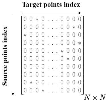
Figure 3: Similarity Matrix.’*’ represent the Correntropy values.

3.2.1 SM Matrix is a sparse Matrix

Since at every iteration we initialize the values to zeros and based on Equ. 7 we fill the Correntropy similarity values at only specified location, the matrix is sparse. Line 7 and 8 in Algorithm 1 clearly indicated that we update only those indices in the Source and the Target point indexes which are close to each other. Fig. 3 shows a simple structure of the similarity matrix.

3.2.2 The rows and columns are linearly independent

Every element in the SM matrix or $\textbf{SM}(i,j)$ represents the Correntropy relationship between the $i$th Source point and the $j$th Target point. Since we are computing the similarity of only the closest point from the Source index to the Target index, every other indices that particular row/column is intuitively zero. This clearly means for every row index in the Source point set there is only one component in the Target dataset with a similarity metric which assures one to one relationship between every Source point to every Target point. The points in the Source point set are transformed based on this rotation matrix after every iteration. This process is repeated every iteration and one can find that the number of points with closer similarity metric $(\sim 1)$ increases. Fig 4 shows that as the iterations increases the rank approaches $N$.

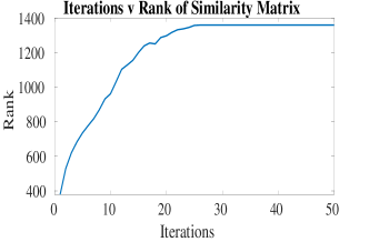
Figure 4: As the iterations increases, the rank of the matrix approaches $N$. Here $N$ is 1360.

3.2.3 Similarity Matrix is a Mirror-Symmetric Matrix.

From Equ. 7, one can verify that if the matrix is diagonally separated, then it’s a mirror image of each other (Mirror-Symmetric Matrices) which means $\textbf{SM}=\textbf{SM}^{T}$.

4 Results

4.1 Evaluation on Datasets with no outliers.

We validated our approach on 3 simple and well known datasets: the Bunny Rabbit, the Happy Buddha and the Dragon dataset. In addition, we have also performed our evaluation on a Lidar dataset (KITTI dataset) since it captures data on a large scale. We perform our experiment on Intel i7 2.Ghz CPU with 32 Gb of RAM. We implemented our approach in the PCL library (version 1.9) and released our code in the github repository ( https://github.com/aralab-unr/CoSM-ICP). In this section, we did not add any random outliers, and we introduce random rotation and translation between the Source and the Target point sets. First we capture a sample pcd file and transform the acquired point cloud with a random transformation matrix where all the individual components of the transformation matrix were randomly generated with different seeds (we assume throughout the paper that the units for angle are in radians). We name the original point cloud as read from the pcd file as Target and the randomly transformed point cloud as the Source. The problem statement is to find the relative transformation between the Source and the Target such that the Source is aligned with the Target. For the above steps, the algorithm is described in Algorithm  2.

1:function ReadPCDFile(’filename.pcd’,$\mathbb{P_{t}}$). $\triangleright$ Read the PCD file and name it as a Target.

2:     $a_{ax}$= Random angular component along the X-axis (-6.28 to 6.28 radians).

3:     $a_{ay}$= Random angular component along the Y-axis (-6.28 to 6.28 radians).

4:     $a_{az}$= Random angular component along the Z-axis (-6.28 to 6.28 radians).

5:     $tr_{tx}$= Random translation along the X-axis.

6:     $tr_{ty}$= Random translation along the Y-axis.

7:     $tr_{tz}$= Random translation along the Z-axis.

8:     $\textbf{M}\leftarrow\textbf{GenerateTransformationMatrix}(a_{ax},a_{ay},a_{az},tr_{tx},tr_{ty},tr_{tz}$)

9:     $\mathbb{P_{s}}\leftarrow\mathbb{TransformPointCloud}(\mathbb{P_{t}},\mathbb{M}$)

10:     return $\mathbb{P_{s}}$ $\triangleright$ Return the transformed point cloud and name it as Source.

11:end function

Algorithm 2 Transform the point cloud with a Random Transformation Matrix.

(a)

(b)

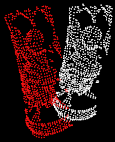
(c)

Figure 5: Rotated and translated point cloud (white is the original point cloud (Target), and Red is the transformed point cloud (Source)) with rotation of $(r,p,y)=(0.314,0,0)$ and translation of $0.05$ unit in the z-axis. (a) shows the bunny rabbit point cloud down sampled using voxel grid filtering of leaf size $0.005$. (b) shows the dragon point cloud down sampled using voxel grid filtering of leaf size $0.005$. (c) shows the happy buddha point cloud down sampled using voxel grid filtering of leaf size $0.005$.

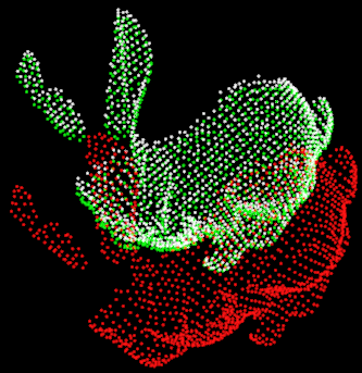
(a)

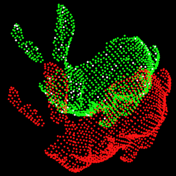
(b)

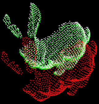
(c)

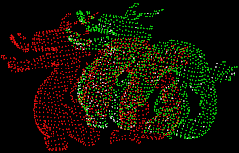
(d)

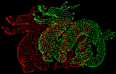
(e)

(f)

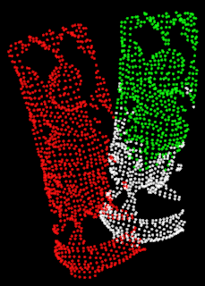
(g)

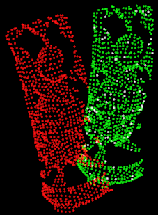
(h)

(i)

Figure 6: Transformation from Source to Target: $(r,p,y,x,y,z)=(0.314,0,0,0,0,0.05)$. White point cloud: Original point cloud (Target). Red point cloud: Source point cloud and Green point cloud : Source transformed point cloud after 10 iterations using (a) ICP Standard SVD (RMSE: 6.25494e-06) (b) ICP Point to Plane (RMSE: 2.77175e-16) and (c) CoSM ICP (RMSE: 3.34226e-06) on the Bunny Rabbit dataset. Similarly we perform 50 iterations on the Dragon dataset using (d) ICP Standard SVD (RMSE: 2.86089e-14 ) (e) ICP Point to Plane (RMSE: 3.93822e-16) and (f) CoSM ICP (RMSE: 2.72838e-15) and 35 iterations on the Happy Buddha dataset using (g) ICP Standard SVD (RMSE: 1.72851e-13) (h) ICP Point to Plane (RMSE: 3.91357e-16) and (i) CoSM ICP (RMSE: 2.46336e-14).

To validate our approach on the datasets, we collected the results on a simple scenario where the Source is transformed manually with a simple transformation matrix which has less variation in rotation and translation ($(r,p,y,x,y,z)=(0.314,0,0,0,0,0.05)$). We reduce the number of point clouds to decrease the computational time by performing Voxel grid filtering (leaf size $0.005$) on the point clouds. The original number of points in the bunny point cloud sets is 40256 points, and after applying voxel grid filtering we get the number of points reduced to 1360 points. Similarly for the Dragon dataset, the original number of points is 43467 points, and after voxel grid filtering the number of points is reduced to 1593 points. The original number of points for the Happy Buddha dataset is 76166 points, and after voxel grid filtering we get 1090 points. The Source and the Target point clouds for the datasets are shown in Fig. 5.

After applying few iterations, our approach aligns equally well (RMSE: 2.46336e-14) in comparison to the well known methods like ICP with standard SVD method (RMSE: 6.25494e-06) and ICP point to plane (RMSE: 2.77175e-16). The results for different datasets are shown in Fig. 6. We compared the Root Mean Square Error (RMSE) on this particular transformation and we see that ICP point to plane converges faster than other methods including ours (in 50 iterations). Fig. 7 shows the RMSE comparisons of different approaches on different datasets for this simple transformation. In this example, ICP point to plane seems to converge faster than our method since the rotation and the translation component is very small. The next step is to evaluate how well our method performs as compared to the other methods when the rotation is large.

Fig. 9 shows the results of different approaches including ours when the rotation and the translation component of the transformation matrix in quite large. In this example we use the Bunny Rabbit dataset where the Source is transformed from the Target as:

$(r,p,y,x,y,z)=(-1.32811,-5.87854,2.12814,-0.874,-0.433,0.221)$.

Clearly the translation component is small as compared to the rotation component. In this example, our method performs well in comparison to the other methods with RMSE as 4.76074e-06 in our method after 20 iterations. It clearly shows that the Source is aligned very well with our approach where as in other methods the Source failed to align with the Target point cloud. We compared the RSME results with other approaches like GICP, NDT and ICP-nonlinear [24, 25, 26]. Fig 8 shows the RMSE results for various methods on the Bunny Rabbit dataset. It is clear that our method performs well in comparison to others. In addition, Table 2 shows the RMSE comparison of various methods applied on the Bunny Rabbit dataset with various rotation and translation.

In Fig. 10 we use the Dragon dataset where the Source is transformed from the Target as:

$(r,p,y,x,y,z)=(2.39318,-5.02554,-2.69076,0.000,-0.003,0.003)$.

Again, our method performs well in comparison to other methods with RMSE as 8.66664e-08 in our method after 25 iterations. We arrive at a similar conclusion that the Source is aligned very well with our approach where as in other methods the Source failed to align with the Target point cloud. Fig. 11 shows the RMSE results for various methods on the Dragon dataset. In addition, Table 3 shows the RMSE comparison of various methods applied on the Dragon dataset with various rotation and translation.

In Fig. 12 we use the Happy Buddha dataset where the Source is transformed from the Target as $(r,p,y,x,y,z)=(-4.50504,1.31677,4.83251,-0.023,-0.019,-0.008)$. Again, our method performs well in comparison to the rest of the methods with RMSE as 2.26675e-06 in our method after 25 iterations. We arrive at a similar conclusion that the Source is aligned very well with our approach where as in other methods the Source failed to align with the Target point cloud. Fig 13 shows the RMSE results for various methods on Dragon dataset. In addition, Table 4 shows the RMSE comparison of various methods applied on Dragon dataset with various rotation and translation.

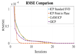
(a)

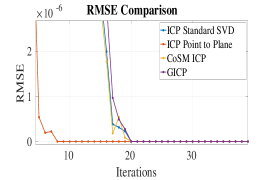
(b)

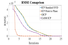
(c)

Figure 7: Convergence of different Registration Methods (ICP Standard SVD, ICP point to plane, GICP and CoSM ICP) on different datasets on the simple transformation ($(r,p,y,x,y,z)=(pi/10,0,0,0,0,0.05)$). (a) Shows RMSE comparison on Bunny Rabbit dataset. (b) Shows RMSE comparison on the Dragon dataset. (c) RMSE comparison on the Happy Buddha dataset.

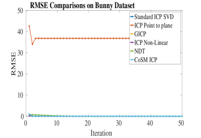
(a)

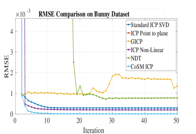
(b)

Figure 8: RMSE comaprison of various methods on the Bunny Rabbit dataset. (b) shows the zoomed in version of (a).

Table 2: RMSE comparison of different methods with different values of rotation and translation after 50 iterations on Bunny Rabbit dataset. Note: Rotation component is in radians.

Transformation(r,p,y,x,y,z)	ICP Standard SVD	ICP Point to Plane	GICP	ICP Non-Linear	NDT	CoSM ICP
(2.39384,-2.57132,4.66973,0.876204,-2.83931,2.68268)	0.000428388	88.0656	0.0011591	0.000206335	15.5141	1.81066e-13
(6.10518,-0.249119,2.41527,1.99458,8.99637,1.20097)	0.000274292	268.684	81.2352	0.000301596	81.2352	3.09602e-13
(1.17438,-5.95203,-4.13622,4.6532,6.28659,0.0542642)	0.000177495	147.987	58.9048	2.69103e-11	58.9048	1.75634e-13
(-0.866749,-2.6182,-0.318386,-2.1561,-1.25001,-4.8753)	0.000283007	859.114	28.7628	0.000244988	28.7628	1.98801e-13
(5.08434,-3.9644,-2.66895,2.45251,-6.82633,1.41512)	0.000471378	58.1505	55.996	1.54e-11	55.996	2.63875e-13

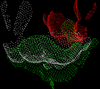
(a)

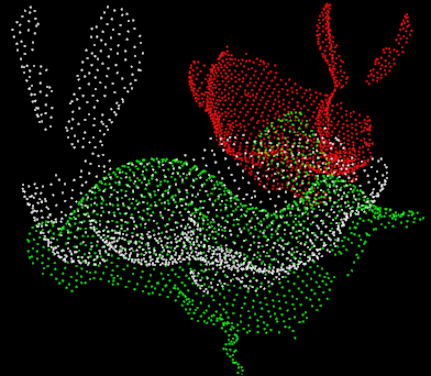
(b)

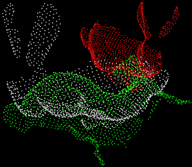
(c)

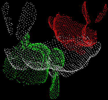
(d)

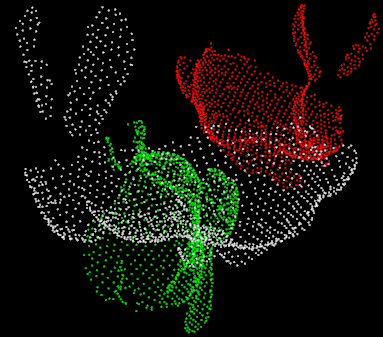
(e)

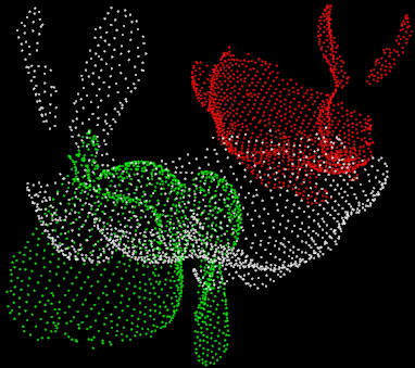
(f)

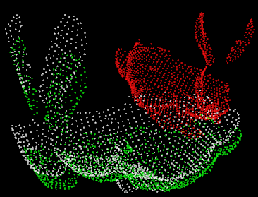
(g)

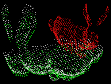
(h)

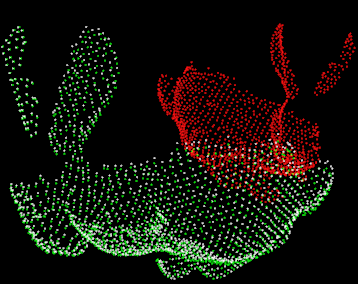
(i)

Figure 9: White Point Cloud: Original Point Cloud (Target). Red Point Cloud: Source point cloud. Green Point Cloud: Source transformed point cloud after applying iterations. Source is transformed from the Target as ($(r,p,y,x,y,z)=(-1.32811,-5.87854,2.12814,-0.874,-0.433,0.221)$). (a)-(c) shows the convergence of the Source point clouds after 5, 10 and 20 iterations using the standard ICP, respectively (RMSE after 20 iterations is 0.000358474). (d)-(f) shows the same using ICP Point to Plane (RMSE after 20 iterations is 0.00216325). (g)-(i) shows the same using CoSM ICP (RMSE after 20 iterations is 4.76074e-06).

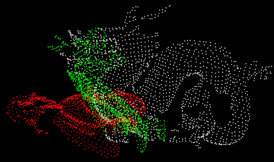
(a)

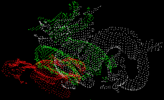
(b)

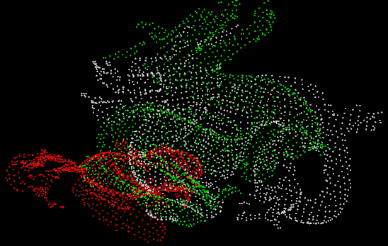
(c)

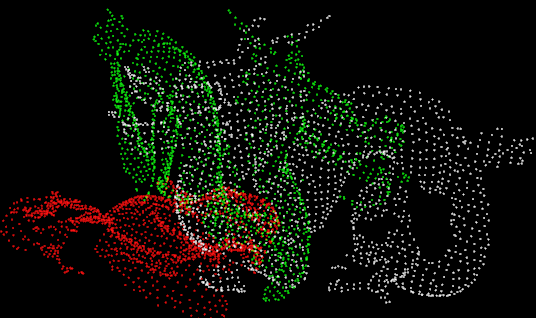
(d)

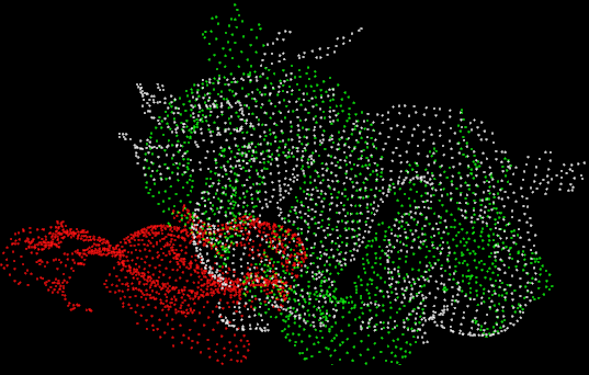
(e)

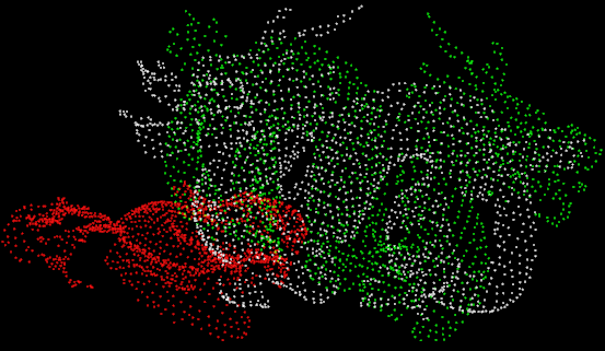
(f)

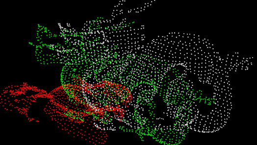
(g)

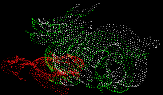
(h)

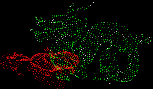
(i)

Figure 10: White point cloud: Original Point Cloud (Target). Red point cloud: Source point cloud. Green point cloud: shows the Source transformed point cloud after applying different registration methods. Source is transformed from the Target as ($(r,p,y,x,y,z)=(2.39318,-5.02554,-2.69076,0.000,-0.003,0.003)$). (a)-(c) shows the convergence of the Source point clouds after 5, 10 and 25 iterations using the standard ICP, respectively (RMSE after 25 iterations is 0.000198014). (d)-(f) shows the same using ICP Point to Plane (RMSE after 25 iterations is 0.000136451). (g)-(i) shows the same using CoSM ICP (RMSE after 25 iterations is 8.66664e-08).

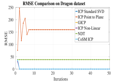
(a)

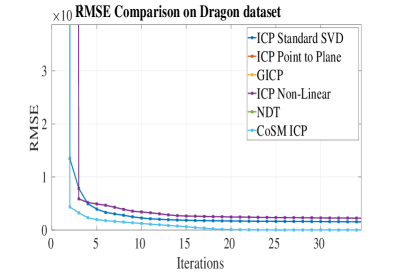
(b)

Figure 11: RMSE comparison of various methods on Dragon dataset. (b) shows the zoomed in version of (a).

Table 3: RMSE comparison of different methods with different values of rotation and translation (from Source to Target) after 50 iterations on Dragon dataset. Note: Rotation component is in radians

Transformation(r,p,y,x,y,z)	ICP Standard SVD	ICP Point to Plane	GICP	ICP Non-Linear	NDT	CoSM ICP
(-2.8152,-2.09474,-2.48844,5.66472,6.31125,-9.44663)	0.000167091	638.278	156.91	0.000159398	156.9	4.19748e-13
(0.429847,2.60943,3.61045,3.6405,-1.63246,7.60966)	0.00016037	325.136	73.1995	0.000224256	73.1995	1.25329e-13
(-2.78018,2.15172,-4.43629,-4.52232,-9.42573,-2.54953)	0.000142098	3015.76	115.142	0.000162551	115.142	3.78298e-13
(1.75465,-1.56088,-1.70889,2.33321,6.13018,3.79368)	0.000142188	26.6913	56.4895	0.000224482	56.4895	1.94386e-13
(-3.72204,1.05945,2.34622,-4.65481,9.74086,3.64636)	0.000159037	115.65	127.159	126.91	127.159	4.19583e-13

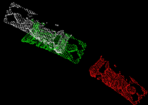
(a)

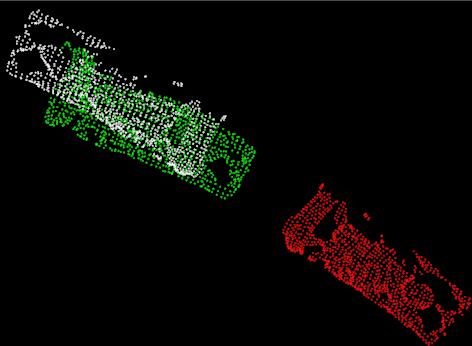
(b)

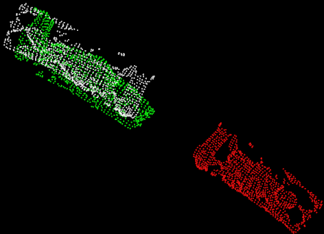
(c)

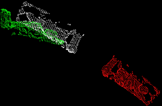
(d)

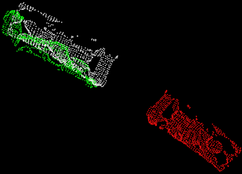
(e)

(f)

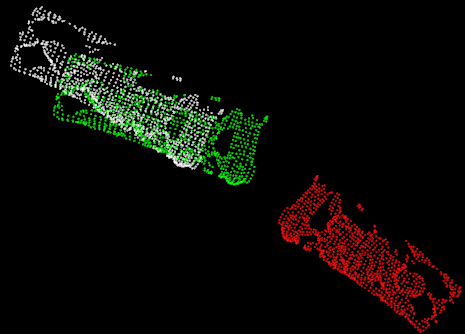
(g)

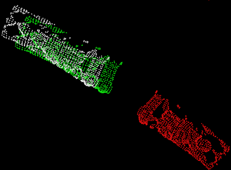
(h)

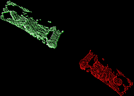
(i)

Figure 12: White point cloud: Original point cloud (Target). Red point cloud: Source point cloud. Green: Source transformed point cloud after applying different registration methods. Source is transformed from the Target as ($(r,p,y,x,y,z)=(-4.50504,1.31677,4.83251,-0.023,-0.019,-0.008)$). (a)-(c) shows the convergence of the Source point clouds after 5, 10 and 25 iterations using the standard ICP, respectively (RMSE after 25 iterations is 0.000128905). (d)-(f) shows the same using ICP Point to Plane (RMSE after 25 iterations is 0.000124717). (g)-(i) shows the same using CoSM ICP (RMSE after 25 iterations is 2.26675e-06).

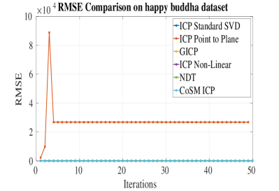
(a)

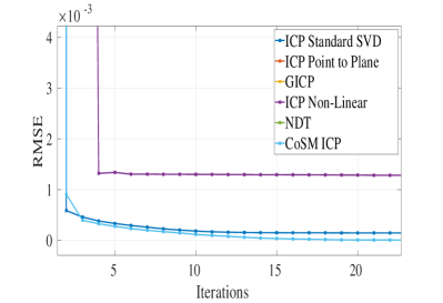
(b)

Figure 13: RMSE comparison of various methods on the Happy Buddha dataset. (b) shows the zoomed in version of (a).

Table 4: RMSE comparison of different methods with different values of rotation and translation (from Source to Target)after 50 iterations on the Happy Buddha dataset. Note: Rotation component is in radians

Transformation(r,p,y,x,y,z)	ICP Standard SVD	ICP Point to Plane	GICP	ICP Non-Linear	NDT	CoSM ICP
(0.429847,2.60943,3.61045,3.6405,-1.63246,7.60966)	0.00016037	325.136	73.1995	0.000224256	73.1995	1.25329e-13
(-1.58692,-5.66055,-4.80461,-7.03304,0.718292,2.77415)	0.000142378	469.843	55.5392	0.00016041	55.5392	1.41924e-13
(-2.79112,4.31946,-2.15715,2.44105,2.03992,-1.87023)	0.000121835	39.1843	0.0018519	0.000133238	11.981	7.99904e-14
(-0.744191,-1.86187,-1.78262,-4.61717,1.79701,-7.04776)	0.000192252	81.0697	71.9632	0.000192185	71.9632	1.80283e-13
(5.17263,1.57234,1.9238,-0.263428,5.05962,-2.27954)	0.000157366	116.57	27.6866	0.000182242	27.6866	1.38844e-13

For evaluating on the Lidar dataset we applied a voxel grid filtering of leaf size $1.5$. The original point cloud size is 115150 points and after voxel grid filtering we get 1497 points. In Fig. 12 we use the Lidar dataset where the Source is transformed from the Target as $(r,p,y,x,y,z)=(-4.27108,-0.505914,0.0988647,10.938,-10.532,17.832)$. Again, our method performs well in comparison to the rest of the methods with RMSE as 2.26675e-06 in our method after 25 iterations. We arrive at a similar conclusion that the Source is aligned very well with our approach where as in other methods the Source failed to align with the Target point cloud. Fig 15 shows the RMSE results for various methods on the Lidar dataset. In addition, Table 5 shows the RMSE comparison of various methods applied on the Lidar dataset with various rotation and translation.

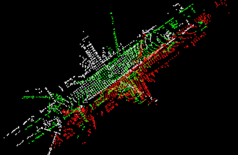
(a)

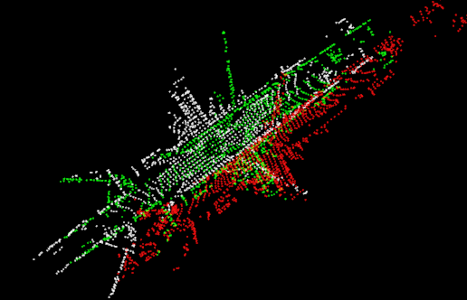
(b)

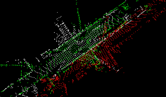
(c)

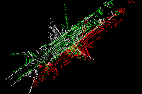
(d)

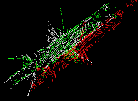
(e)

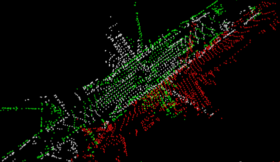
(f)

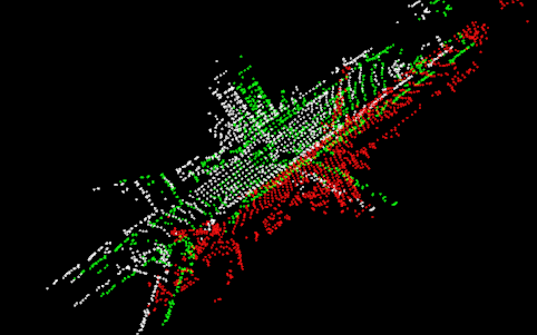
(g)

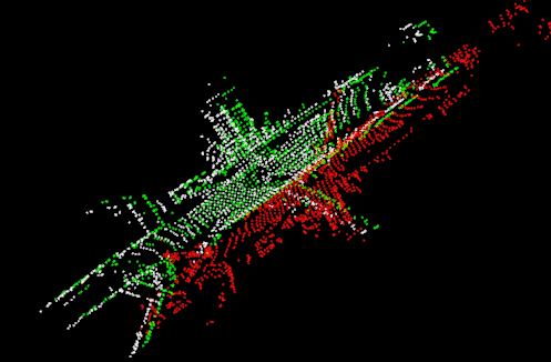
(h)

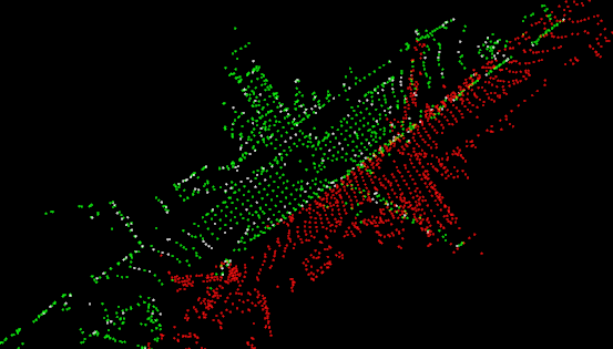
(i)

Figure 14: (From KITTI dataset) White point cloud: Original Point Cloud(Target). Red point cloud: Source point cloud and Green point cloud: Source transformed point cloud after applying different registration methods. Source is transformed from the Target as ($(r,p,y,x,y,z)=(-4.27108,-0.505914,0.0988647,10.938,-10.532,17.832)$). (a)-(c) shows the convergence of the Source point clouds after 7, 15 and 33 iterations using the standard ICP, respectively (RMSE after 33 iterations is 13.7695). (d)-(f) shows the same using ICP Point to Plane (RMSE after 33 iterations is 12.6385). (g)-(i) shows the same using CoSM ICP (RMSE after 25 iterations is 1.01689e-08).

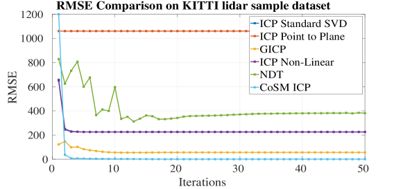
Figure 15: RMSE comparison of various methods on the KITTI Lidar dataset.

Table 5: RMSE comparison of different methods with different values of rotation and translation (from Source to Target)after 50 iterations on the KITTI Lidar dataset. Note: Rotation component is in radians

Transformation(r,p,y,x,y,z)	ICP Standard SVD	ICP Point to Plane	GICP	ICP Non-Linear	NDT	CoSM ICP
(4.23443,-5.64022,-3.13665,-2.2485,-1.19326,-9.12248)	16.1754	371.296	38.1373	16.1762	274.547	3.4779e-08
(3.64853,-3.29044,-5.13981,0.991908,-5.06315,4.75733)	16.9795	480.78	321.312	23.8551	432.754	3.20148e-08
(-5.78829,0.576843,1.91183,0.640607,6.7615,3.82172)	194.469	513.454	225.474	194.581	257.164	4.47064e-08
(-1.0146,-0.427581,-3.42779,7.22804,-7.6078,-0.806072)	10.2524	286.673	18.9515	10.266	24.5575	2.83469e-08
(0.149154,4.33846,1.82095,-2.5633,-0.377752,-1.20834)	16.8181	1010.43	248.244	17.2776	258.734	4.46591e-08

4.2 Evaluation on datasets with outliers.

In this section we evaluated our approach in cases where the data has outliers. We randomly injected data values at random indexes in the Source point set. The algorithm for injecting random outliers is shown in Algorithm 3.

1:function InjectOutliers($\mathbb{P_{s}}$).$\triangleright$ Read the Source point cloud data.

2:     $ridx$= Pick random index in the Source point set.

3:     $tr_{tx}$= Random translation along the X-axis.

4:     $tr_{ty}$= Random translation along the Y-axis.

5:     $tr_{tz}$= Random translation along the Z-axis.

6:     $\mathbb{P_{s}}[ridx].x=\mathbb{P_{s}}[ridx].x+tr_{tx}$

7:     $\mathbb{P_{s}}[ridx].y=\mathbb{P_{s}}[ridx].y+tr_{ty}$

8:     $\mathbb{P_{s}}[ridx].z=\mathbb{P_{s}}[ridx].z+tr_{tz}$

9:     return $\textbf{P}_{s}$ $\triangleright$ Return the transformed point cloud and name it as Source.

10:end function

Algorithm 3 Transform the point cloud with a Random Transformation Matrix.

In this experiment we selected the percentage of points in the Source dataset to be affected by outliers. We added the outliers after performing voxel grid filtering of leaf size $0.005$ since one can still encounter outliers after pre-processing the data. The Source point cloud is transformed from the Target point cloud with the transformation $(r,p,y,x,y,z)=(-1.32811,-5.87854,2.12814,-0.874,-0.433,0.221)$. The Source point cloud is indeed affected by outliers, and we compare the results with different approaches on different datasets when 10% ,25% and 50% of the Source data points are affected.

We compared our approach with other methods as well. Table 6 shows the RMSE comparison with other datasets where 10% of the Source dataset (after voxel grid filtering) is is affected. Clearly, our methods outperforms other approaches under various rotations and translations. Our results are consistent and keeps performing better even when 25% and 50% of the Source dataset are affected as shown in 7 and 8.

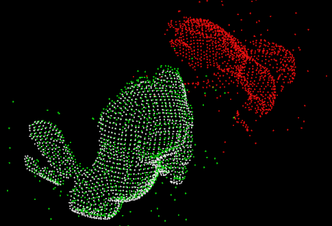
(a)

(b)

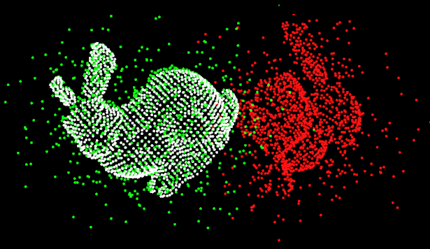
(c)

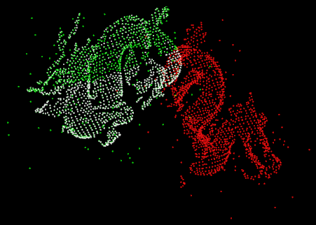
(d)

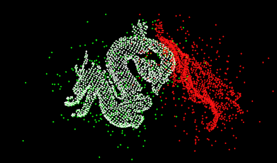
(e)

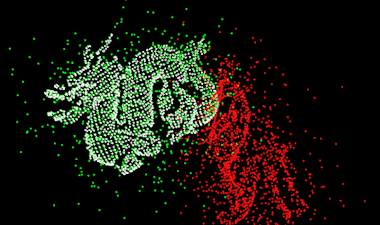
(f)

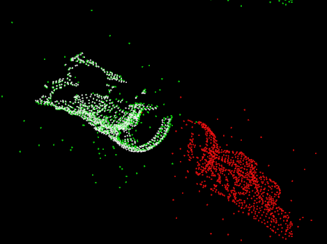
(g)

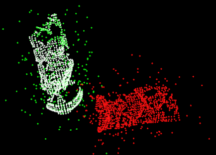
(h)

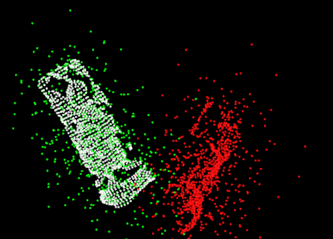
(i)

Figure 16: CoSM Results when Source is infected with noise. White point cloud: Original Point Cloud (Target). Red point cloud: Infected Source point cloud. Green point cloud: Source transformed point cloud after applying iterations. Transformation from Source to Target: ($(r,p,y,x,y,z)=(1.6585448,0.6090677,-1.204856,0.00,-0.003,0.003)$). (a),(b) and (c) shows the result of CoSM ICP on Bunny dataset when 10%, 25% and 50%of the data is affected with outliers. Their respective RMSE’s are $8.64002e-05$,$0.000203088$ and $0.000384025$. (d),(e) and (f) shows the result of CoSM ICP on the Dragon dataset when 10%, 25% and 50%of the data is affected with outliers. Their respective RMSE’s are $6.91792e-05$,$0.000163833$ and $0.000368516$. (g),(h) and (i) shows the result of CoSM ICP on the Happy Buddha dataset when 10%, 25% and 50%of the data is affected with outliers. Their respective RMSE’s are $9.29047e-05$,$0.000205528$ and $0.000386966$. For each case we performed around 30 iterations.

Table 6: (10% of the Source data contains outliers) RMSE comparison of different methods with different values of rotation and translation (from Source to Target) after 50 iterations on different datasets. Note: Rotation component is in radians

Bunny Dataset
Transformation(r,p,y,x,y,z)	ICP Standard SVD	ICP Point to Plane	GICP	ICP Non-Linear	NDT	CoSM ICP
(-2.36822,-0.726873,-5.69612,7.08856,-2.68581,7.63531)	0.000411328	711.375	114.581	0.000269638	114.581	6.15845e-05
(-2.67216,3.73756,-0.902484,-9.27928,-4.0282,4.09878)	0.000257389	374.895	0.000460177	23.8551	119.48	7.70252e-05
(-1.56059,4.39878,-2.80893,-3.94166,-3.10092,-3.34176)	0.000527419	304.884	37.13	0.000487805	37.13	8.26112e-05
Dragon Dataset
(0.177274,-3.62568,5.47677,0.852604,-5.3915,-9.91804)	0.000220957	76.301	128.455	0.000246111	128.455	6.49243e-05
(-0.620232,-5.82563,3.78543,4.85066,2.74563,-8.42101)	0.000270745	45.484	101.049	23.8551	101.049	7.94277e-05
(-1.53521,4.48718,-0.388112,-7.74233,5.42215,-6.44992)	0.00021795	241.345	125.922	0.000223478	125.922	7.67165e-05
Happy Buddha Dataset
(-2.83367,-1.24896,2.98587,2.69059,3.34046,-4.41227)	0.000176202	19.1229	36.8922	0.000212469	36.8922	7.10533e-05
(-2.47527,-5.65213,-3.30425,-3.8167,8.95128,-9.03962)	0.000210153	598.839	174.049	0.000217757	174.049	8.03656e-05
(3.05982,-0.897597,-1.43556,1.60636,1.22125,7.01582)	0.000171509	146.972	52.0521	0.000202291	52.0521	7.24014e-05

Table 7: (25% of the Source data contains outliers) RMSE comparison of different methods with different values of rotation and translation (from Source to Target) after 50 iterations on different datasets. Note: Rotation component is in radians

Bunny Dataset
Transformation(r,p,y,x,y,z)	ICP Standard SVD	ICP Point to Plane	GICP	ICP Non-Linear	NDT	CoSM ICP
(1.55693,-1.11205,4.17676,-6.05252,1.66971,5.82581)	0.000426784	1175.52	71.583	0.000365769	71.583	0.000187812
(5.65505,4.15868,-3.27751,9.31612,-5.23313,-5.55587)	0.000346638	3286.84	0.000410574	144.696	144.696	0.000167037
(-2.55584,-4.76118,3.16486,-7.20725,3.99654,-7.30791)	0.000447408	1343.79	117.165	0.000552115	117.165	0.000216027
Dragon Dataset
(6.25758,2.3638,-2.88282,-7.36544,-6.20769,-7.92445)	0.000294534	67.9046	156.303	0.000286822	156.303	0.000168995
(3.76055,2.28707,4.29734,-8.8644,-6.40219,1.19919)	0.000255092	115.102	120.245	0.000292728	120.245	0.000158364
(4.63246,-4.08457,-1.65193,-9.97667,-4.37054,1.77417)	0.000354324	174.437	119.75	0.000263999	119.75	0.000162741
Happy Buddha Dataset
(-1.20164,-2.47146,4.2161,1.29076,7.69533,-6.64823)	0.000295019	116.015	98.0711	0.000298207	98.0711	0.000194422
(-1.14973,-4.81181,3.44981,9.95025,9.69451,8.84972)	0.000266775	103.766	269.094	0.000262239	269.094	0.000177326
(-2.78376,3.84551,-5.11847,-0.469235,-7.93148,-7.98029)	0.000269701	116.321	127.049	0.000269828	127.049	0.0001856

Table 8: (50% of the Source data contains outliers) RMSE comparison of different methods with different values of rotation and translation (from Source to Target) after 50 iterations on different datasets. Note: Rotation component is in radians

Bunny Dataset
Transformation(r,p,y,x,y,z)	ICP Standard SVD	ICP Point to Plane	GICP	ICP Non-Linear	NDT	CoSM ICP
(4.21267,-5.1913,0.510754,4.78028,-3.81009,-8.99842)	0.000555246	176.793	118.74	0.000705962	118.74	0.000367226
(-1.90501,2.94602,-4.15732,-4.38121,-8.43926,0.951326)	0.000533201	1644.03	91.374	0.000535398	91.374	0.000364791
(-3.88617,5.23854,-4.81381,2.95017,-6.77983,-2.26068)	0.000615907	83.6865	61.5916	0.000610313	61.5916	0.00036124
Dragon Dataset
(-4.41725,-2.40238,-0.642351,3.74842,-9.32348,-9.14091)	0.000487516	188.167	185.885	0.000510906	185.885	0.000372615
(3.29757,5.37519,4.68352,5.59739,-1.76298,-7.59656)	0.000362955	487.439	90.1547	0.000516225	90.1547	0.000327693
(-2.27986,-2.66004,-5.61896,-9.89552,-2.83092,4.9319)	0.000520534	91.5809	127.933	0.000472107	127.933	0.000380396
Happy Buddha Dataset
(5.4771,1.17243,-0.67022,-8.42324,-5.29389,-3.70151)	0.000462191	510.054	111.689	0.000489964	111.689	0.000384029
(1.77436,-2.70017,-4.70393,1.9514,4.74639,-8.0765)	0.000478957	128.078	90.493	0.000489046	90.493	0.000383038
(-3.01961,2.91297,-5.51066,6.01917,4.29907,5.78239)	0.000486108	155.204	86.8654	0.00173299	86.8654	0.000399139

4.3 Effect of $\sigma$.

As shown in the previous section, the registration works well when the value of $\sigma$ is 100. With lower values of $\sigma$ like 0.01 it aligned well for small rotation and translation, however for large rotation and translation between the Source and the Target it took a large number of iterations to converge. For even smaller values of $\sigma$ like 0.001, and for larger rotation and translation, alignment did take place. Moreover, the iterations was larger ($\sim 500$), and the computed transformation was prone to errors.

5 Discussion

We have found that using a Correntropy Relationship matrix proved to be very effective in the problem of registration. Through experiments we have evaluated that our approach is not only robust to large rotation and translation, but also robust to outliers. We have compared our approach to other state of the art methods like GICP, NDT, ICP Non-Linear etc. and proved it’s efficiency under large transformation matrices. It is quite important to note that the size of the Correntropy Matrix is dependent on the size of the dataset, which means that if we have larger datasets, our approach would be computationally very expensive for each iteration ($\sim 7ms$ for a datset of size 10000 points for each iteration). In addition to our previously mentioned results, we have also evaluated on different datasets using multiple runs. We define a run such that in each run, we generate a random transformation matrix and we compute a transformation matrix from randomly generated translation and rotation components and transform the original point cloud (which we call it as Target) to another point cloud (which we call it as Source). We then employ several state of the art methods like GICP, NDT , ICP Non-Linear NDT and CoSM ICP iteratively on the Source point cloud. In this case we perform the iteration 50 times during each run and collect the final RMSE’s from each of the methods. The components of the random transformation matrix (translation and rotations ($x,y,z,r,p,y$)) are generated independently with different seeds (seeds are defined by the system’s clock). The mean for all the components is zero. The standard deviation for the translation components along $x,y,z$ is 10, where as for the angular components it is 6.28317 radians (360 degrees) along each axes. This guarantees that we could potentially cover all the possible orientation along all axes. On the Bunny dataset we found that ICP Point to Plane had a very large RMSE ( mean RMSE for ICP Point to Plane is $1.9668e+03$ in 100 runs) which means the Source dataset was not at all aligned to the Target dataset at all. However GICP and NDT better than ICP Point to Plane in most of the cases (mean RMSE of GICP in 100 runs is $75.6727$ and the mean RMSE of NDT in 100 runs is $76.2536$). However in certain transformations GICP and NDT performs well with RMSE of $8.8582e-04$ and $5.6122e-04$ respectively. On the other hand if we compare the average RMSE of Standard ICP, ICP Non-linear and CoSM ICP we see that their average RMSE’s in 100 runs is $2.4156e-04$, $2.3781e-04$ and $3.2489e-07$ respectively. It is very evident that CoSM ICP is better than the other approaches (by more than $\sim 100\%$). Fig 17(a) shows the distribution of errors (RMSE’s) of various methods in 100 runs on the Bunny Rabbit dataset. Fig. 17(b) shows the RMSE deviation of Standard ICP, ICP Non-Linear and CoSM ICP. In the Dragon dataset the average RMSE’s of Standard ICP, ICP Point to Plane, GICP, ICP Non-Linear, NDT and CoSM ICP is $1.1372e-04$, $177.0397$, $86.8183$, $1.4154$, $87.5327$ and $2.6989e-13$ respectively. In this case as well CoSM outperformed the other approaches by more than $\sim 100\%$. It is again evident from Fig. 18(a) and Fig. 18(b). On the Happy buddha dataset, the average RMSE’s for Standard ICP, ICP Point to Plane, GICP, ICP Non-Linear, NDT and CoSM ICP is $9.4830e-05$, $414.0633$, $93.0712$, $1.1289e-04$, $93.3621$ and $5.6055e-13$ respectively in 100 runs. Again it is validated that CoSM ICP performs better than the rest of the approaches by more than $\sim 100\%$. Fig. 19(a) and Fig. 19(b) clearly validates our claim for the happy buddha dataset. Readers can note that the top and the bottom of the box plot shown represent the $25^{th}$ and $75^{th}$ percentiles respectively and the middle red line shows the median of the error (average RMSE’s) across 100 runs.

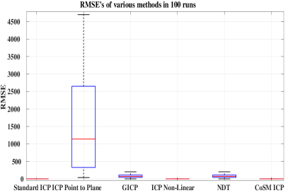
(a)

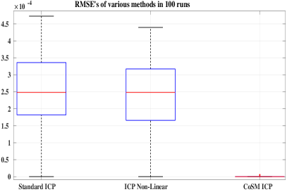
(b)

Figure 17: Average RMSE’s of various methods in 100 runs (Bunny Rabbit dataset). Each run consists of random rotation and translation between the Source and the Target.

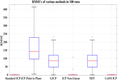
(a)

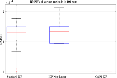
(b)

Figure 18: Average RMSE’s of various methods in 100 runs (Dragon dataset). Each run consist of random rotation and translation between the Source and the Target.

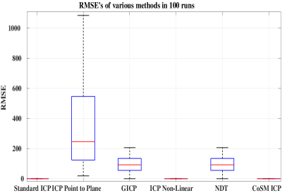
(a)

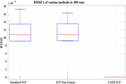
(b)

Figure 19: Average RMSE’s of different methods in 100 runs (Happy Buddha dataset). Each run consist of random rotation and translation between the Source and the Target.

It is significant to note that our approach has proved beneficial in solving the registration problem under various rotations and translations as compared to other well-known methods. We encourage the community to validate our approach on their own datasets.

6 Conclusions and Future Work

One of the key things we have addressed is to find an accurate estimate of the transformation between the Source and the Target point clouds under various rotations and translations. In this work, we have verified our approach in various datasets, where the Source is transformed from the Target using various randomly generated transformation matrices. Through the obtained results we can see that our method has performed better than the other state of the art approaches. In addition, we also evaluate our approach when the Source dataset is affected by noise generated with random intensity and affecting random data points. In this scenario as well, we have verified that our proposed approach has outperformed most of the other state of the art approaches where the ‘infected’ Source dataset is transformed randomly from the Target datset. We strongly insist our readers to evaluate our approach located in our Github repository. In addition to our current approach, we also aim to evaluate our approach in SLAM where the poses computed from our approach can be used to localize a robot (both aerial and ground robot) as well as build a map of the environment. For further evaluation, we plan to test our approach in the well-known KITTI SLAM dataset and other online datasets.

References

- [1] A. Singandhupe, H. M. La, A review of slam techniques and security in autonomous driving, in: 2019 Third IEEE International Conference on Robotic Computing (IRC), 2019, pp. 602–607. doi:10.1109/IRC.2019.00122.
- [2] C. Cadena, L. Carlone, H. Carrillo, Y. Latif, D. Scaramuzza, J. Neira, I. Reid, J. J. Leonard, Past, present, and future of simultaneous localization and mapping: Toward the robust-perception age, IEEE Trans. on Robotics 32 (6) (2016) 1309–1332. doi:10.1109/TRO.2016.2624754.
-
[3]
K. S. Arun, T. S. Huang, S. D. Blostein,
Least-squares fitting of
two 3-d point sets, IEEE Trans. Pattern Anal. Mach. Intell. 9 (5) (1987)
698–700.
doi:10.1109/TPAMI.1987.4767965.
URL https://doi.org/10.1109/TPAMI.1987.4767965 - [4] P. J. Besl, N. D. McKay, A method for registration of 3-d shapes, IEEE Transactions on Pattern Analysis and Machine Intelligence 14 (2) (1992) 239–256.
- [5] K.-L. Low, Linear least-squares optimization for point-to-plane icp surface registration.
- [6] J. Zhang, S. Singh, Visual-lidar odometry and mapping: Low drift, robust, and fast, in: IEEE Intern. Conf. on Robotics and Automation (ICRA), Seattle, WA, 2015.
- [7] T. Y. Tang, D. J. Yoon, F. Pomerleau, T. D. Barfoot, Learning a Bias Correction for Lidar- only Motion Estimation, 15th Conf. on Computer and Robot Vision (CRV).
- [8] K. Tateno, F. Tombari, I. Laina, N. Navab, Cnn-slam: Real-time dense monocular slam with learned depth prediction, 2017 IEEE Conference on Computer Vision and Pattern Recognition (CVPR) (2017) 6565–6574.
- [9] A. Sehgal, A. Singandhupe, H. M. La, A. Tavakkoli, S. J. Louis, Lidar-monocular visual odometry with genetic algorithm for parameter optimization, in: G. Bebis, R. Boyle, B. Parvin, D. Koracin, D. Ushizima, S. Chai, S. Sueda, X. Lin, A. Lu, D. Thalmann, C. Wang, P. Xu (Eds.), Advances in Visual Computing, Springer International Publishing, Cham, 2019, pp. 358–370.
- [10] C. Choy, W. Dong, V. Koltun, Deep global registration, in: Proceedings of the IEEE Conference on Computer Vision and Pattern Recognition, 2020.
- [11] H. Yang, J. Shi, L. Carlone, Teaser: Fast and certifiable point cloud registration, ArXiv abs/2001.07715.
- [12] Q.-Y. Zhou, J. Park, V. Koltun, Fast global registration, in: B. Leibe, J. Matas, N. Sebe, M. Welling (Eds.), Computer Vision – ECCV 2016, Springer International Publishing, Cham, 2016, pp. 766–782.
- [13] A. Singandhupe, H. M. La, Mcc-ekf for autonomous car security, Proceedings of the 4th IEEE International Conference on Robotic Computing (IRC).
-
[14]
Z. Wu, H. Chen, S. Du, M. Fu, N. Zhou, N. Zheng,
Correntropy
based scale icp algorithm for robust point set registration, Pattern
Recognition 93 (2019) 14 – 24.
doi:https://doi.org/10.1016/j.patcog.2019.03.013.
URL http://www.sciencedirect.com/science/article/pii/S0031320319301116 -
[15]
S. Fakoorian, A. Mohammadi, V. Azimi, D. Simon,
Robust Kalman-Type Filter for
Non-Gaussian Noise: Performance Analysis With Unknown Noise Covariances,
Journal of Dynamic Systems, Measurement, and Control 141 (9).
arXiv:https://asmedigitalcollection.asme.org/dynamicsystems/article-pdf/141/9/091011/4497081/ds\_141\_09\_091011.pdf,
doi:10.1115/1.4043054.
URL https://doi.org/10.1115/1.4043054 - [16] X. Zhang, L. Jian, M. Xu, Robust 3d point cloud registration based on bidirectional maximum correntropy criterion, PloS one 13 (5) (2018) e0197542.
- [17] G. Xu, S. Du, D. Cui, S. Zhang, B. Chen, X. Zhang, J. Xue, Y. Gao, Precise point set registration using point-to-plane distance and correntropy for lidar based localization, in: 2018 IEEE Intelligent Vehicles Symposium (IV), IEEE, 2018, pp. 734–739.
- [18] X. Zhang, L. Jian, M. Xu, Robust 3d point cloud registration based on bidirectional maximum correntropy criterion, PLOS ONE 13 (2018) e0197542. doi:10.1371/journal.pone.0197542.
- [19] G. Xu, S. Du, D. Cui, S. Zhang, B. Chen, X. Zhang, J. Xue, Y. Gao, Precise point set registration using point-to-plane distance and correntropy for lidar based localization, in: 2018 IEEE Intelligent Vehicles Symposium (IV), 2018, pp. 734–739. doi:10.1109/IVS.2018.8500525.
- [20] R. Izanloo, S. A. Fakoorian, H. S. Yazdi, D. Simon, Kalman filtering based on the maximum correntropy criterion in the presence of non-gaussian noise., in: CISS, IEEE, 2016, pp. 500–505.
-
[21]
B. Chen, X. Liu, H. Zhao, J. C. Principe,
Maximum
correntropy kalman filter, Automatica 76 (2017) 70 – 77.
doi:https://doi.org/10.1016/j.automatica.2016.10.004.
URL http://www.sciencedirect.com/science/article/pii/S000510981630396X - [22] J. C. Principe, Information Theoretic Learning: Renyi’s Entropy and Kernel Perspectives, 1st Edition, Springer Publishing Company, Incorporated, 2010.
- [23] J. Principe, J. Iii, Information-theoretic learning, Advances in unsupervised adaptive filtering.
- [24] A. Segal, D. Hähnel, Generalized-icp, 2009. doi:10.15607/RSS.2009.V.021.
- [25] P. Biber, W. Strasser, The normal distributions transform: a new approach to laser scan matching, in: Proceedings 2003 IEEE/RSJ International Conference on Intelligent Robots and Systems (IROS 2003) (Cat. No.03CH37453), Vol. 3, 2003, pp. 2743–2748 vol.3. doi:10.1109/IROS.2003.1249285.
-
[26]
A. W. Fitzgibbon,
Robust
registration of 2d and 3d point sets, Image and Vision Computing 21 (13)
(2003) 1145–1153, british Machine Vision Computing 2001.
doi:https://doi.org/10.1016/j.imavis.2003.09.004.
URL https://www.sciencedirect.com/science/article/pii/S0262885603001835