Tight distance-dependent estimators for screening two-center and three-center short-range Coulomb integrals over Gaussian basis functions

Abstract

We derive distance-dependent estimators for two-center and three-center electron repulsion integrals over a short-range Coulomb potential, $\mathrm{erfc}(\omega r_{12})/r_{12}$. These estimators are much tighter than one based on the Schwarz inequality and can be viewed as a complement to the distance-dependent estimators for four-center short-range Coulomb integrals and for two-center and three-center full Coulomb integrals previously reported. Because the short-range Coulomb potential is commonly used in solid-state calculations, including those with the HSE functional and with our recently introduced range-separated periodic Gaussian density fitting, we test our estimators on a diverse set of periodic systems using a wide range of the range-separation parameter $\omega$. These tests demonstrate the robust tightness of our estimators, which are then used with integral screening to calculate periodic three-center short-range Coulomb integrals with linear scaling in system size.

I Introduction

Accurate estimators of electron repulsion integrals (ERIs) over pairs of charge densities are essential ingredients for large-scale electronic structure calculations using Gaussian-type orbitals (GTOs). Screening based on these estimators can be used to avoid computing negligible integrals and thereby achieve reduced computational scaling in both Hartree-Fock (HF) Coulomb White et al. (1994); Strout and Scuseria (1995); White et al. (1996); White and Head-Gordon (1996); Strain, Scuseria, and Frisch (1996); Challacombe, Schwegler, and Almlöf (1996) and exchange Schwegler and Challacombe (1996); Challacombe and Schwegler (1997); Ochsenfeld, White, and Head-Gordon (1998) problems and electron correlation methods Schütz, Lindh, and Werner (1999); Lambrecht, Doser, and Ochsenfeld (2005); Doser et al. (2009); Maurer et al. (2013). Despite its simplicity and behavior as a rigorous upper bound, the well-known Schwarz inequality Dyczmons (1973); Häser and Ahlrichs (1989); Gill, Johnson, and Pople (1994) does not capture the decay of ERIs with the distance between the charge densities. Lambrecht, Doser, and Ochsenfeld (2005) This has led to the development of tight distance-dependent integral estimators for conventional four-center ERIs, Lambrecht, Doser, and Ochsenfeld (2005); Doser et al. (2009); Maurer et al. (2012, 2013) as well as two-center and three-center ERIs, Hollman, Schaefer, and Valeev (2015); Valeev and Shiozaki (2020) which appear in many semi-empirical methods Peels and Knizia (2020) and the density fitting method Whitten (1973); Dunlap, Connolly, and Sabin (1979); Mintmire and Dunlap (1982).

In addition to the bare Coulomb operator, other potentials commonly appear in the ERIs. Savin and Flad (1995); Leininger et al. (1997); Adamson, Dombroski, and Gill (1999); Iikura et al. (2001); Heyd, Scuseria, and Ernzerhof (2003); Toulouse, Colonna, and Savin (2004); Yanai, Tew, and Handy (2004); Refaely-Abramson et al. (2013); Lutsker, Aradi, and Niehaus (2015) One of the most widely used is the Coulomb potential attenuated by the complementary error function,

$$g_{\omega}(r_{12})=\frac{\mathrm{erfc}(\omega r_{12})}{r_{12}},$$ (1)

which we henceforth refer to as the short-range (SR) Coulomb potential. The SR Coulomb potential reduces to the full Coulomb potential for $\omega\to 0$ and $\delta(r_{12})$ for $\omega\to\infty$, thus connecting the full ERIs to the overlap integrals between two charge distributions. Jung et al. (2005); Reine et al. (2008) The four-center SR ERIs are used in calculating the screened exchange energy in the Heyd-Scuseria-Ernzerhof (HSE) exchange correlation functional Heyd, Scuseria, and Ernzerhof (2003, 2006), whose application in solids is motivated by the unphysical behavior of long-range exchange in metals. Distance-dependent estimators for the four-center SR ERIs were first derived by Izmaylov and co-workers Izmaylov, Scuseria, and Frisch (2006), which have since been used for the efficient evaluation of the HSE exchange integrals Guidon et al. (2008); Guidon, Hutter, and VandeVondele (2009); Shang, Li, and Yang (2011); Beuerle, Kussmann, and Ochsenfeld (2017).

The two-center and three-center SR ERIs were first used in local density fitting for finite systems Jung et al. (2005); Reine et al. (2008) and screening was done according to the Schwarz inequality Reine et al. (2008), which is suboptimal, as discussed above. More recently, the two of us introduced a global density fitting scheme for periodic systems Ye and Berkelbach (2021) where the use of range separation, in the spirit of Ewald summation, results in the appearance of two-center and three-center SR ERIs, which has motivated us to find tight estimators for integral screening. To the best of our knowledge, there has been no systematic studies on the estimators for two-center and three-center SR ERIs, which we aim to address in this work.

Although our estimators are expected to work equally well in both finite and periodic calculations, we choose periodic systems in this work to demonstrate the practical use of the estimators. We develop algorithms for efficiently evaluating the periodic two-center and three-center SR ERIs, where the estimators are used to truncate the infinite lattice sum and avoid the calculation of unimportant integrals. We show that highly controlled accuracy of the computed periodic integrals can be achieved over a wide range of $\omega$ values. We analyze how the computational scaling of the lattice sum changes with $\omega$ and show that the computational cost scales linearly with the system size.

This paper is organized as follows. In Section II.1, we establish our notation, and in Sections II.2, II.3 and II.4, we present the derivation of the distance-dependent estimators for two-center and three-center SR ERIs, first for primitive GTOs and then extended to contracted GTOs. In Section II.5, we describe our algorithms for efficiently computing the periodic two-center and three-center SR ERIs, where the estimators derived in previous sections play the key role to truncate the infinite lattice sum and perform integral screening. After giving computational details in Section III, we present numerical data in Section IV to assess the tightness and accuracy of our estimators. We also discuss the favorable computational scaling for the lattice sum enabled by using the estimators. In Section V, we conclude by pointing out a few future directions.

II Theory

II.1 Notations

In this work, a primitive GTO (pGTO) with principal angular momentum $l$, projected angular momentum $m$, and Gaussian exponent $\zeta_{a}$ is defined as Schlegel and Frisch (1995)

$$\phi_{alm}(\bm{r})=N_{al}r^{l}y_{lm}(\hat{\bm{r}})\mathrm{e}^{-\zeta_{a}r^{2}}$$ (2)

where

$$N_{al}=\sqrt{\frac{2(2\zeta_{a})^{l+3/2}}{\Gamma(l+3/2)}}$$ (3)

is the radial normalization factor, and

$$\begin{split}y_{lm}(\theta,\varphi)&=\sqrt{\frac{2l+1}{4\pi}\frac{(l+|m|)!}{(l-|m|)!}(2-\delta_{m0})}\\ &\qquad\times P_{l}^{|m|}(\cos\theta)\left\{\begin{split}\cos(m\varphi)\quad&m\geq 0,\\ \sin(|m|\varphi)\quad&m<0.\end{split}\right.\end{split}$$ (4)

is the angular part of a real solid harmonic function. A contracted GTO (cGTO) is a linear combination of a group of concentric pGTOs that have the same angular momentum but differ in their Gaussian exponents,

$$\chi_{\mu}(\bm{r};\bm{R})=\sum_{a}C_{a\mu}\phi_{al_{\mu}m_{\mu}}(\bm{r}-\bm{R}).$$ (5)

A shell refers to a set of GTOs differing only by the projected angular momentum $m$. There are $2l+1$ orbitals in a shell of angular momentum $l$. Throughout this work, we consider atomic orbital (AO) basis sets that contain both primitive and contracted GTOs and auxiliary basis sets that are all primitive GTOs. Unless otherwise stated, the two-center ERIs are over two auxiliary orbitals, and the three-center ERIs are over the product of two AOs (in the bra) and an auxiliary orbital (in the ket).

In the derivation below, we omit the labels for angular momentum and use $\phi_{a}\equiv\phi_{al_{a}m_{a}}$ in cases without possible confusion. We also omit the radial normalization factor $N_{al}$, which is multiplicative and can be readily recovered if necessary.

II.2 Two-center SR ERIs over pGTOs

Consider the SR ERIs over two pGTOs

$$J_{ab}(\bm{R})=\int\mathrm{d}\bm{r}_{1}\int\mathrm{d}\bm{r}_{2}\,\phi_{a}(\bm{r}_{1}-\bm{R})\phi_{b}(\bm{r}_{2})g_{\omega}(r_{12})$$ (6)

where we choose a coordinate system where the ket orbital is centered at the origin. The ERI $J_{ab}(\bm{R})$ may take $(2l_{a}+1)\times(2l_{b}+1)$ possible values $\{J_{ab}^{m_{a}m_{b}}(\bm{R})\}$, each corresponding to a specific choice of $(m_{a},m_{b})$. Our goal in this section is to derive an approximate formula for estimating the shell-wise Frobenius norm

$$\|J_{ab}^{m_{a}m_{b}}(\bm{R})\|_{\mathrm{F}}\equiv\mathcal{J}_{ab}(R)=\bigg{\{}\sum_{m_{a}=-l_{a}}^{l_{a}}\sum_{m_{b}=-l_{b}}^{l_{b}}\big{[}J_{ab}^{m_{a}m_{b}}(\bm{R})\big{]}^{2}\bigg{\}}^{1/2}$$ (7)

which only depends on the distance $R$ between the two orbitals due to the rotational invariance of the Frobenius norm.

II.2.1 The $O_{0}v_{0}$ estimator

We begin by considering the simplest case of two $s$-type orbitals. The exact expression for Eq. 6 in this special case is well-known Izmaylov, Scuseria, and Frisch (2006)

$$J_{a(l_{a}=0)b(l_{b}=0)}=\frac{O_{a0}O_{b0}}{R}\big{[}\mathrm{erfc}(\eta_{ab\omega}^{1/2}R)-\mathrm{erfc}(\eta_{ab}^{1/2}R)\big{]}$$ (8)

where

$$\eta_{ab} =(\zeta_{a}^{-1}+\zeta_{b}^{-1})^{-1},$$ (9a)

$$\eta_{ab\omega} =(\eta_{ab}^{-1}+\omega^{-2})^{-1},$$ (9b)

and $O_{a0}=\pi/(2\zeta_{a}^{2/3})$ is the charge of $\phi_{a(l_{a}=0)}$. Since the complementary error function decays exponentially with its argument and $\eta_{ab}>\eta_{ab\omega}$, only the first term of Eq. 8 survives at large $R$. This leads to what we call the $O_{0}v_{0}$ estimator

$$\mathcal{J}^{O_{0}v_{0}}_{ab}(R)=O_{a0}O_{c0}\frac{\mathrm{erfc}(\eta_{ab\omega}^{1/2}R)}{R},$$ (10)

which can be applied for orbitals of arbitrary angular momenta. The name comes from interpreting Eq. 10 as two charges or zeroth-order multipoles (hence $O_{0}$) interacting via an effective SR Coulomb potential

$$v_{0}(\eta_{ab\omega},R)=g_{\eta_{ab\omega}^{1/2}}(R)=\frac{\mathrm{erfc}(\eta_{ab\omega}^{1/2}R)}{R}.$$ (11)

Despite the formal similarity between the $O_{0}v_{0}$ estimator and the classical Coulomb interaction between two point charges, we emphasize that the interpretation above is phenomenological rather than physical. As pointed out by Izmaylov and co-workers Izmaylov, Scuseria, and Frisch (2006), the fact that $v_{0}$ depends on the orbital exponents [i.e., not simply $\mathrm{erfc}(\omega R)/R$] means that Eq. 10 is not a classical multipole interaction. Nonetheless, we will see below that the phenomenological interpretation applies for orbitals of higher angular momentum, too.

The $O_{0}v_{0}$ estimator shows no dependence on the orbital angular momentum $l$. One thus expects it to be accurate only for integrals over e.g., $s$- and $p$-type orbitals.

II.2.2 The $O_{l}v_{l}$ estimator

Let us now consider the general case of Eq. 6 with arbitrary angular momenta, $l_{a}$ and $l_{b}$. The real-space double integral in Eq. 6 can be turned into a single integral in reciprocal space by using the Fourier transforms from Appendix A; the result is

$$\begin{split}J_{ab}^{m_{a}m_{b}}(\bm{R})&=\mathrm{i}^{l_{ab}}2^{-l_{ab}+1}\pi^{-1}\gamma_{al_{a}}\gamma_{bl_{b}}\times\\ &\quad{}\sum_{l=|l_{a}-l_{b}|}^{l_{ab}}\sum_{m=-l}^{l}\mathrm{i}^{l}T_{l_{a}m_{a},l_{b}m_{b}}^{lm}y_{lm}(\hat{\bm{R}})\times\\ &\quad{}\big{[}I(R;l_{ab},l,\eta_{ab})-I(R;l_{ab},l,\eta_{ab\omega})\big{]}\end{split}$$ (12)

where $l_{ab}=l_{a}+l_{b}$, $\gamma_{al}=(\pi/\zeta_{a})^{3/2}\zeta_{a}^{-l}$,

$$T_{l_{a}m_{a},l_{c}m_{c}}^{lm}=\int\mathrm{d}\hat{\bm{q}}\,y_{lm}(\hat{\bm{q}})y_{l_{a}m_{a}}(\hat{\bm{q}})y_{l_{c}m_{c}}(\hat{\bm{q}})$$ (13)

is the coefficient for angular momentum coupling, and

$$I(R;L,l,\eta)=\int_{0}^{\infty}\mathrm{d}q\,q^{L}\mathrm{e}^{-q^{2}/(4\eta)}j_{l}(qR),$$ (14)

with $j_{l}(x)$ the spherical Bessel function.

To make progress, we show in Appendix B that the contribution from Eq. 14 to Eq. 12 is asymptotically $l$-independent. As a result, we evaluate Eq. 14 with a convenient choice, $l=L$, and obtain a simple, closed-form expression

$$I(R;L,L,\eta)=2^{L-1}\pi^{1/2}R^{-(L+1)}\Gamma(L+1/2,\eta R^{2}),$$ (15)

where $\Gamma(x,y)$ is the upper incomplete gamma function. With this result, in the large $R$ limit, Eq. 12 simplifies to

$$J_{ab}^{m_{a}m_{b}}(\bm{R})\approx\frac{\gamma_{al_{a}}\gamma_{bl_{b}}}{\pi^{1/2}R^{l_{ab}+1}}\Gamma(l_{ab}+1/2,\eta_{ab\omega}R^{2})\Theta_{l_{a}m_{a},l_{b}m_{b}}^{lm}(\hat{\bm{R}})$$ (16)

where

$$\Theta_{l_{a}m_{a},l_{b}m_{b}}^{lm}(\hat{\bm{R}})=\mathrm{i}^{l_{ab}}\sum_{l=|l_{a}-l_{b}|}^{l_{ab}}\sum_{m=-l}^{l}\mathrm{i}^{l}T_{l_{a}m_{a},l_{b}m_{b}}^{lm}y_{lm}(\hat{\bm{R}})$$ (17)

collects the angular dependence on $\bm{R}$. For estimating the Frobenius norm, $\mathcal{J}_{ab}(R)$, it is sufficient to use

$$\|\Theta_{l_{a}m_{a},l_{b}m_{b}}^{lm}(\hat{\bm{R}})\|_{\mathrm{F}}\approx\frac{\sqrt{(2l_{a}+1)(2l_{b}+1)}}{4\pi}.$$ (18)

This simplifies Eq. 16 to what we call the $O_{l}v_{l}$ estimator

$$\mathcal{J}_{ab}^{O_{l}v_{l}}(R)=O_{al_{a}}O_{bl_{b}}\frac{\Gamma(l_{ab}+1/2,\eta_{ab\omega}R^{2})}{\pi^{1/2}R^{l_{ab}+1}},$$ (19)

where

$$O_{al}=\frac{\pi\sqrt{2l+1}}{2\zeta_{a}^{l+3/2}}$$ (20)

is the orbital multipole of arbitrary angular momentum. As for the $O_{0}v_{0}$ estimator, the name $O_{l}v_{l}$ comes from interpreting Eq. 19 phenomenologically as two multipoles (hence $O_{l}$) interacting via an effective potential

$$v_{l_{ab}}(\eta_{ab\omega},R)=\frac{\Gamma(l_{ab}+1/2,\eta_{ab\omega}R^{2})}{\pi^{1/2}R^{l_{ab}+1}}.$$ (21)

For $l_{a}=l_{b}=0$, both the orbital multipole Eq. 20 and the effective potential Eq. 21 reduce to their counterpart in Section II.2.1. Thus, the $O_{l}v_{l}$ estimator Eq. 19 is a direct generalization of the $O_{0}v_{0}$ estimator to arbitrary orbital angular momenta. Equation 19 also parallels the estimator for two-center Coulomb ERIs obtained by Valeev and Shiozaki based on a multipole analysis Valeev and Shiozaki (2020).

In addition to $O_{0}v_{0}$ and $O_{l}v_{l}$, one can readily write down two other estimators

$$\mathcal{J}_{ab}^{O_{l}v_{0}}(R)=O_{al_{a}}O_{bl_{b}}v_{0}(\eta_{ab\omega},R),$$ (22)

$$\mathcal{J}_{ab}^{O_{0}v_{l}}(R)=O_{a0}O_{b0}v_{l_{ab}}(\eta_{ab\omega},R)$$ (23)

which consider the $l$-dependence for the orbital multipoles alone ($O_{l}v_{0}$) or the effective potential alone ($O_{0}v_{l}$), respectively. In Section IV.1, we will see that only the $O_{l}v_{l}$ estimator is tight in all cases, and the comparison with the other three estimators help understand the importance of a correct treatment of the orbital angular momenta.

II.3 Three-center SR ERIs over pGTOs

Consider the SR ERIs over three pGTOs

$$\begin{split}J_{abc}(\bm{R}_{a},\bm{R}_{b})&=\int\mathrm{d}\bm{r}_{1}\int\mathrm{d}\bm{r}_{2}\,\phi_{a}(\bm{r}_{1a})\phi_{b}(\bm{r}_{1b})\phi_{c}(\bm{r}_{2})g_{\omega}(r_{12})\end{split}$$ (24)

where $\bm{r}_{1a}=\bm{r}_{1}-\bm{R}_{a}$, $\bm{r}_{1b}=\bm{r}_{1}-\bm{R}_{b}$, and we choose a coordinate system where the ket orbital is centered at the origin. The ERI $J_{abc}(\bm{R}_{a},\bm{R}_{b})$ can take $(2l_{a}+1)\times(2l_{b}+1)\times(2l_{c}+1)$ possible values $\{J_{abc}^{m_{a}m_{b}m_{c}}(\bm{R}_{a},\bm{R}_{b})\}$, each corresponding to a specific choice of $(m_{a},m_{b},m_{c})$. Our goal is again to derive an approximate formula for estimating the shell-wise Frobenius norm,

$$\mathcal{J}_{abc}(\bm{R},\bm{d})=\bigg{\{}\sum_{m_{a}=-l_{a}}^{l_{a}}\sum_{m_{b}=-l_{b}}^{l_{b}}\sum_{m_{c}=-l_{c}}^{l_{c}}\big{[}J_{abc}^{m_{a}m_{b}m_{c}}(\bm{R}_{a},\bm{R}_{b})\big{]}^{2}\bigg{\}}^{1/2},$$ (25)

where on the left side of the equation we have switched to the representation of the bra separation, $\bm{d}=\bm{R}_{b}-\bm{R}_{a}$, and the bra-ket separation, $\bm{R}=(\zeta_{a}\bm{R}_{a}+\zeta_{b}\bm{R}_{b})/\zeta_{ab}$, where $\zeta_{ab}=\zeta_{a}+\zeta_{b}$. Unlike the two-center case [Eq. 7], $\mathcal{J}_{abc}(\bm{R},\bm{d})$ in general depends on both the norm and the orientation of the relevant position vectors.

Our starting point for deriving an estimator for Eq. 25 is to turn the bra product distribution, $\rho_{ab}(\bm{r}_{1})=\phi_{a}(\bm{r}_{1a})\phi_{b}(\bm{r}_{1b})$, into a sum of individual pGTOs, which will then reduce a three-center ERI into a sum of two-center ERIs, for which the $O_{l}v_{l}$ estimator (19) is a good approximation.

II.3.1 The ISF estimator

We begin with the simple case, $l_{a}=l_{b}=0$, where the Boys relation Boys (1950); Szabo and Ostlund (1996) can be used,

$$\phi_{a(l_{a}=0)}(\bm{r}_{1a})\phi_{b(l_{b}=0)}(\bm{r}_{1b})=y_{00}\mathrm{e}^{-\eta_{ab}d^{2}}\phi_{\zeta_{ab}(l=0)}(\bm{r}_{1\bm{R}}),$$ (26)

which expresses the well-known result that the product of two $s$-type pGTOs is another $s$-type pGTO with an exponent $\zeta_{ab}$, located at the charge center $\bm{R}$, and scaled in magnitude by $y_{00}\mathrm{e}^{-\eta_{ab}d^{2}}$. Using this identity, a three-center ERI with two $s$-type bra orbitals and an arbitrary ket orbital is

$$J_{a(l_{a}=0)b(l_{b}=0)c}(\bm{R},\bm{d})=\frac{\mathrm{e}^{-\eta_{ab}d^{2}}}{2\pi^{1/2}}J_{\zeta_{ab}(l_{ab}=0)c}(\bm{R}).$$ (27)

Approximating $J_{\zeta_{ab}(l_{ab}=0)c}(\bm{R})$ by the $O_{l}v_{l}$ estimator (19) leads to what we call the ISF estimator for three-center SR ERIs

$$\mathcal{J}_{abc}^{\mathrm{ISF}}(R,d)=\frac{\mathrm{e}^{-\eta_{ab}d^{2}}}{2\pi^{1/2}}O_{\zeta_{ab}0}O_{cl_{c}}v_{l_{c}}(\eta_{abc\omega},R)$$ (28)

where

$$\eta_{abc\omega}=(\eta_{ab}^{-1}+\zeta_{c}^{-1}+\omega^{-2})^{-1}.$$ (29)

The name comes from the fact that Eq. 28 can be viewed as a direct extension of the work by Izmaylov, Scuseria, and Frisch Izmaylov, Scuseria, and Frisch (2006) (ISF), who derived the exact expression for a four-center SR ERI over all $s$-type pGTOs using the Boys relation (26) and then used it as an estimator for orbitals of arbitrary angular momentum. Here in Eq. 28, we include the $l$-dependence for the ket orbital via our two-center estimator (19).

Note that the ISF estimator (and all other three-center estimators derived below) depends on only the norm of $\bm{R}$ and $\bm{d}$. The lack of angular dependence here is not a crucial issue as applications such as integral screening are nearly exclusive to medium to large bra-ket separation $R$, where the effect of the orbital orientation is relatively weak.

II.3.2 The ISF$Q_{0}$ estimator

For non-$s$-type orbitals, the bra product is in general a sum of $l_{ab}+1$ terms according to the Gaussian product theorem (GPT) Besalú (2011); Fermann and Valeev (2020),

$$\phi_{a}(\bm{r}_{1a})\phi_{b}(\bm{r}_{1b})=\mathrm{e}^{-\eta_{ab}d^{2}}\sum_{l=0}^{l_{ab}}\sum_{m=-l}^{l}L_{l_{a}m_{a},l_{b}m_{b}}^{lm}(\bm{d},\zeta_{a},\zeta_{b})\phi_{\zeta_{ab}(l)}(\bm{r}_{1\bm{R}}),$$ (30)

where $\{L_{l_{a}m_{a},l_{b}m_{b}}^{lm}\}$ are related to the Talmi coefficients whose explicit expression can be derived in various ways. Matsuoka (1998a, b) Equation 30 can also be viewed as expanding a product distribution by its multipole components, and the ISF estimator (28) keeps only the lowest-order multipole, i.e., the charge, of the bra product distribution.

One way to include the effect of higher-order multipoles is using the Schwarz $Q$-integral Häser and Ahlrichs (1989) generalized for a SR Coulomb potential

$$\mathcal{Q}_{ab}(d)=\|V_{abab}(\bm{d})\|_{\mathrm{F}}^{1/2}$$ (31)

where

$$\begin{split}V_{abab}(\bm{d})&=\int\mathrm{d}\bm{r}_{1}\int\mathrm{d}\bm{r}_{2}\,\phi_{a}(\bm{r}_{1})\phi_{b}(\bm{r}_{1}-\bm{d})\\ &\hskip 60.00009pt\times\phi_{a}(\bm{r}_{2})\phi_{b}(\bm{r}_{2}-\bm{d})g_{\omega}(r_{12})\end{split}$$ (32)

and the Frobenius norm is again shell-wise

$$\|V_{abab}(\bm{d})\|_{\mathrm{F}}=\bigg{\{}\sum_{m_{a}=-l_{a}}^{l_{a}}\sum_{m_{b}=-l_{b}}^{l_{b}}\sum_{m_{a}^{\prime}=-l_{a}}^{l_{a}}\sum_{m_{b}^{\prime}=-l_{b}}^{l_{b}}[V_{abab}^{m_{a}m_{b}m_{a}^{\prime}m_{b}^{\prime}}(\bm{d})]^{2}\bigg{\}}^{1/2}.$$ (33)

For the simplest case of two $s$-type pGTOs,

$$\mathcal{Q}_{a(l_{a}=0)b(l_{b}=0)}(d)=\mathrm{e}^{-\eta_{ab}d^{2}}\frac{\sqrt{2}}{\pi^{5/4}}\big{(}\eta_{abab}^{1/2}-\eta_{abab\omega}^{1/2}\big{)}^{1/2}$$ (34)

where $\eta_{abab}=(\zeta_{ab}^{-1}+\zeta_{ab}^{-1})^{-1}=\zeta_{ab}/2$ and $\eta_{abab\omega}=(\eta_{abab}^{-1}+\omega^{-2})^{-1}$. By rewriting the exponential factor $\mathrm{e}^{-\eta_{ab}d^{2}}$ in Eq. 28 using Eq. 34, we obtain what we call the ISF$Q_{0}$ estimator

$$\mathcal{J}_{abc}^{\mathrm{ISF}Q_{0}}(R,d)=\frac{\pi^{3/4}\mathcal{Q}_{ab}(d)O_{cl_{c}}}{\big{[}2(\eta_{abab}^{1/2}-\eta_{abab\omega}^{1/2})\big{]}^{1/2}}v_{l_{c}}(\eta_{abc\omega},R)$$ (35)

We note that Eq. 35 parallels the $QVl$ estimator obtained by Hollman et al. for three-center Coulomb ERIs. Hollman, Schaefer, and Valeev (2015)

II.3.3 The ISF$Q_{l}$ estimator

The ISF$Q_{0}$ estimator amounts to approximating the exact multipole expansion of the bra product distribution (30) by the $l=0$ term with a modified prefactor to capture the overall effect of all higher-order terms. When $\omega$ is small, we expect this to be a good approximation, because the SR Coulomb potential resembles the full Coulomb potential, for which the classical multipole interaction, which decays faster for higher-order multipoles, is a good approximation Lambrecht, Doser, and Ochsenfeld (2005); Maurer et al. (2012). For large $\omega$, however, terms with $l>0$ could be more important due to the incomplete gamma function in the effective potential (21). Using the ISF$Q_{0}$ estimator may cause underestimation in this regime.

While it is possible to consider a full multipole expansion with approximate coefficients (Section II.3.4), a simpler amendment to the ISF$Q_{0}$ estimator is to restore the $l$-dependence and keep only the term of the maximum value. Specifically, we define the ISF$Q_{l}$ estimator as

$$\begin{split}\mathcal{J}^{\mathrm{ISF}Q_{l}}_{abc}(R,d)&=\frac{\pi^{3/4}\mathcal{Q}_{ab}(d)O_{cl_{c}}}{2^{1/2}}\\ &\quad{}\times\max_{l}\bigg{\{}\big{(}\eta_{abab}^{l+1/2}-\eta_{abab\omega}^{l+1/2}\big{)}^{-1/2}v_{l+l_{c}}(\eta_{abc\omega},R)\bigg{\}},\end{split}$$ (36)

where the maximization is over $\{0,1,\cdots,l_{ab}\}$ for $d>0$ but $\{|l_{a}-l_{b}|,|l_{a}-l_{b}|+1,\cdots,l_{ab}\}$ for $d=0$ by the properties of angular momentum coupling. We expect ISF$Q_{l}$ to essentially reduce to ISF$Q_{0}$ when $\omega$ is small, but corrects the underestimation of the latter for larger $\omega$.

II.3.4 The ME estimator

In principle, a more accurate account of the multipole expansion (30) needs the GPT coefficients $\{L_{l_{a}m_{a},l_{b}m_{b}}^{lm}\}$. Consider a special case where both $\phi_{a}$ and $\phi_{b}$ are located on the $z$-axis and $m_{a}=m_{b}=0$. In this case, the spherical GTO (2) becomes equivalent to a Cartesian GTO with $z$-component only,

$$\phi_{a(m_{a}=0)}(\bm{r}_{1a})\sim z_{1a}^{l_{a}}\mathrm{e}^{-\zeta_{a}r_{1a}^{2}},$$ (37)

and a similar expression holds for $\phi_{b(m_{b}=0)}(\bm{r}_{1b})$. The product distribution then becomes,

$$\phi_{a(m_{a}=0)}(\bm{r}_{1a})\phi_{b(m_{b}=0)}(\bm{r}_{1b})\sim\mathrm{e}^{-\eta_{ab}d^{2}}\sum_{l=0}^{l_{ab}}L_{l_{a},l_{b}}^{l}z_{1\bm{R}}^{l}\mathrm{e}^{-\zeta_{ab}r_{1\bm{R}}^{2}}$$ (38)

where

$$L_{l_{a},l_{b}}^{l}=\sum_{l^{\prime}=-l}^{l}{}^{{}^{\prime}}{l_{a}\choose l_{a}^{\prime}}{l_{b}\choose l_{b}^{\prime}}d_{a}^{l_{a}-l_{a}^{\prime}}d_{b}^{l_{b}-l_{b}^{\prime}},$$ (39)

gives the GPT coefficients in this special case, where $l_{a}^{\prime}=(l+l^{\prime})/2$, $l_{b}^{\prime}=(l-l^{\prime})/2$, $d_{a}=z_{\bm{R}}-z_{a}$, $d_{b}=z_{\bm{R}}-z_{b}$, and the primed summation means increment by $2$. Now for the general case where $\phi_{a}$ and $\phi_{b}$ are arbitrarily located and have arbitrary $(m_{a},m_{b})$, we can still use Eq. 39 to approximate the GPT coefficients if $d>0$ and $d_{a}$ and $d_{b}$ are chosen to be

$$\begin{split}d_{a}&=-\|\bm{R}_{a}-\bm{R}\|=-(\zeta_{b}/\zeta_{ab})d,\\ d_{b}&=\|\bm{R}_{b}-\bm{R}\|=(\zeta_{a}/\zeta_{ab})d.\end{split}$$ (40)

Using Eqs. 39 and 40 leads to what we call the ME estimator (where “ME” stands for multipole expansion)

$$\begin{split}\mathcal{J}_{abc}^{\mathrm{ME}}(R,d)&=\frac{\mathrm{e}^{-\eta_{ab}d^{2}}O_{cl_{c}}}{2\pi^{1/2}}\sum_{l=0}^{l_{ab}}|L_{l_{a},l_{b}}^{l}(d,\zeta_{a},\zeta_{b})|O_{\zeta_{ab}l}v_{l+l_{c}}(\eta_{abc\omega},R).\end{split}$$ (41)

The case $d=0$, i.e., $\phi_{a}$ and $\phi_{b}$ are concentric, needs special consideration. As mentioned above, the GPT expansion in this case should range from $|l_{a}-l_{b}|$ to $l_{ab}$, while Eqs. 39 and 40 predict all terms except for $l=l_{ab}$ vanish, which leads to a significant underestimation of the true integrals. To obtain a better approximation in this case, we assume a simple structure for the approximate GPT coefficients

$$L_{l_{a},l_{b}}^{l}(d=0,\zeta_{a},\zeta_{b})=\zeta_{ab}^{\alpha l+\beta l_{ab}}f(l_{ab},l)$$ (42)

where $l=|l_{a}-l_{b}|,|l_{a}-l_{b}|+1,\cdots,l_{ab}$, and determine the parameters in Eq. 42 empirically from numerical tests. We found that the following choices work well

$$\alpha=\frac{1}{2},\quad\beta=-\frac{1}{2},\quad f(l_{ab},l)=\bigg{[}\frac{(l_{ab}-1)!}{(l-1)!}\bigg{]}^{1/2}$$ (43)

where we define $(-1)!=1$. The numerical evidence for Eq. 43 is given in Figs. S1 and S2. Equations 42 and 43 together with Eqs. 39 and 40 thus complete the definition of the ME estimator (41) for three-center SR ERIs.

II.4 From primitive to contracted GTOs

The estimators derived above assume all orbitals are pGTOs [Eq. 2]. To apply them for integrals over cGTOs [Eq. 5], we find that a one-term approximation works well in the appropriate large-$R$ limit. In this case, a cGTO, $\chi_{\mu}$, is replaced by its most diffuse pGTO component, $C_{\mu a^{*}}\phi_{a^{*}}$, and

$$\mathcal{J}_{\mu\nu c}(\bm{R},\bm{d})\approx C_{\mu a^{*}}C_{\nu b^{*}}\mathcal{J}_{abc}(\bm{R},\bm{d}),$$ (44)

where $\mathcal{J}_{abc}(\bm{R},\bm{d})$ can be estimated by one of the three-center estimators derived in the previous section. For ISF$Q_{0}$ (35) and ISF$Q_{l}$ (36), the Schwarz-$Q$ integrals can be calculated using the original cGTOs [i.e., $\mathcal{Q}_{\mu\nu}(d)$] to effectively account for the contribution from other pGTOs in the cGTOs.

II.5 Periodic two-center and three-center SR ERIs with screening

As a practical application of the estimators derived above and also a means to test their accuracy, we show how to exploit these estimators to efficiently calculate periodic two-center and three-center SR ERIs. As mentioned in the introduction, these integrals are needed in our recently introduced periodic global density fitting scheme Ye and Berkelbach (2021) and would be needed in a density-fitted implementation of the HSE functional Heyd, Scuseria, and Ernzerhof (2003, 2006), among other possible applications.

II.5.1 Periodic two-center SR ERIs

A periodic system consists of a unit cell and its infinite periodic images, each specified by a lattice translational vector, $\bm{m}$, with $\bm{m}=\bm{0}$ the reference cell. Consider $n$ atom-centered GTOs, $\{\phi_{a}(\bm{r}-\bm{\tau}_{a})\}$, in the reference cell, which, under the periodic boundary condition, become $n$ translationally adapted GTOs

$$\tilde{\phi}_{a}^{\bm{k}}(\bm{r})=\sum_{\bm{m}}\mathrm{e}^{\mathrm{i}\bm{k}\cdot\bm{m}}\phi_{a}(\bm{r}-\bm{m}_{a})$$ (45)

where $\bm{m}_{a}=\bm{m}+\bm{\tau}_{a}$ and $\bm{k}$ is a crystal momentum vector in the first Brillouin zone. In the following, we consider only the $\Gamma$-point Brillouin zone sampling with $\tilde{\phi}_{a}\equiv\tilde{\phi}_{a}^{\bm{k}=\bm{0}}$. This choice corresponds to an in-phase superposition of all cells and hence represents the most challenging case for integral screening. The method can be straightforwardly adapted to use other Brillouin zone sampling schemes.

A periodic two-center SR ERI is

$$L_{ab}=\int_{\Omega}\mathrm{d}\bm{r}_{1}\int\mathrm{d}\bm{r}_{2}\,\tilde{\phi}_{a}(\bm{r}_{1})\tilde{\phi}_{b}(\bm{r}_{2})g_{\omega}(r_{12})=\sum_{\bm{m}}J_{ab}(\bm{m}_{ab_{0}})$$ (46)

where $\Omega$ is the volume of a unit cell, $\bm{m}_{ab_{0}}=\bm{m}_{a}-\bm{\tau}_{b}$, and we used Eqs. 45 and 6 to obtain the second equality, which is an infinite lattice sum. To calculate $L_{ab}$ to a finite precision $\epsilon$, we approximate the lattice sum by an integral over $\bm{R}_{ab}=\bm{m}_{ab_{0}}$ and analyze the error of truncating it at a finite $R_{ab}^{\mathrm{cut}}$

$$\delta L_{ab}\sim\int_{R_{ab}>R_{ab}^{\mathrm{cut}}}\mathrm{d}\bm{R}_{ab}\,J_{ab}(\bm{R}_{ab})\sim f(\eta_{ab\omega},R_{ab}^{\mathrm{cut}})\mathcal{J}_{ab}(R_{ab}^{\mathrm{cut}})$$ (47)

where the form of the multiplicative prefactor $f(\eta_{ab\omega},R_{ab}^{\mathrm{cut}})$ will be derived in Section II.5.3. Equation 47 suggests the cutoff criterion for the lattice sum for $L_{ab}$,

$$f(\eta_{ab\omega},R_{ab}^{\mathrm{cut}})\mathcal{J}_{ab}(R_{ab}^{\mathrm{cut}})=\epsilon,$$ (48)

where $\mathcal{J}_{ab}(R)$ can be estimated using a two-center estimator from Section II.2. Once $R_{ab}^{\mathrm{cut}}$ is determined from Eq. 48,

$$\mathcal{M}_{ab}=\{\bm{m}\,|\,\|\bm{m}_{ab_{0}}\|\leq R_{ab}^{\mathrm{cut}}\}$$ (49)

gives the set of cells needed for calculating $L_{ab}$ to the precision $\epsilon$ via the lattice summation (46). The union $\mathcal{M}_{a}=\cup_{b}\mathcal{M}_{ab}$ then gives all “important” cells for orbital $a$. An algorithm for efficiently calculating the entire $[\mathbf{L}]_{ab}$ matrix based on precomputed cutoffs $\{R_{ab}^{\mathrm{cut}}\}$ and cell data $\{\mathcal{M}_{a}\}$ is presented in Algorithm 1.

Algorithm 1 Eq. 46 by a truncated lattice sum.

Input: $\{R_{ab}^{\mathrm{cut}}\}$, $\{\mathcal{M}_{a}\}$

Initialize: $[\mathbf{L}]_{ab}\leftarrow$ zeros($n$,$n$)

for $a$ in range($n$) do

     for $b$ in range($n$) do

         for $\bm{m}\in\mathcal{M}_{a}$ do

              if $\|\bm{m}_{ab_{0}}\|\leq R^{\mathrm{cut}}_{ab}$ then

                  $L_{ab}\mathrel{+}=J_{ab}(\bm{m}_{ab_{0}})$                             

II.5.2 Periodic three-center SR ERIs

Let $\tilde{\phi}$ and $\tilde{\varphi}$ denote two sets of translationally adapted GTOs [Eq. 45] of size $n_{1}$ and $n_{2}$, respectively (e.g., the sets of periodic AOs and auxiliary basis functions). A periodic three-center SR ERI (using $\Gamma$-point Brillouin zone sampling as discussed above) is

$$\begin{split}L_{abc}&=\int_{\Omega}\mathrm{d}\bm{r}_{1}\int\mathrm{d}\bm{r}_{2}\,\tilde{\phi}_{a}(\bm{r}_{1})\tilde{\phi}_{b}(\bm{r}_{1})\tilde{\varphi}_{c}(\bm{r}_{2})g_{\omega}(r_{12})\\ &=\sum_{\bm{m},\bm{n}}J_{abc}(\bm{m}_{ac_{0}},\bm{n}_{bc_{0}}),\end{split}$$ (50)

where we used Eqs. 24 and 45 to obtain the second equality, which is an infinite double lattice sum. The double lattice sum in Eq. 50 can be rewritten to be over the bra separation, $\bm{d}_{ab}=\bm{m}_{a}-\bm{n}_{b}$, and the bra-ket separation, $\bm{R}_{abc}=\zeta_{ab}^{-1}(\zeta_{a}\bm{m}_{ac_{0}}+\zeta_{b}\bm{n}_{bc_{0}})$,

$$L_{abc}=\sum_{\bm{d}_{ab}}\sum_{\bm{R}_{abc}}J_{abc}(\bm{R}_{abc},\bm{d}_{ab}).$$ (51)

Equation 51 is more convenient for truncation to compute $L_{abc}$ to a finite precision $\epsilon$ as we discuss now.

First, the Schwarz inequality

$$\mathcal{J}_{abc}(\bm{R}_{abc},\bm{d}_{ab})\leq\mathcal{Q}_{ab}(d_{ab})\mathcal{Q}_{c}$$ (52)

with $\mathcal{Q}_{c}=[\mathcal{J}_{cc}(0)]^{1/2}$ gives the decay with $d_{ab}$ regardless of the value for $\bm{R}_{abc}$. We thus follow a similar derivation for Eq. 48 and obtain an equation for the cutoff of $d_{ab}$,

$$f(\eta_{ab},d_{ab}^{\mathrm{cut}})\mathcal{Q}_{ab}(d_{ab}^{\mathrm{cut}})\mathcal{Q}_{c}^{\mathrm{max}}=\epsilon$$ (53)

where $\mathcal{Q}_{c}^{\mathrm{max}}=\max_{c}\mathcal{Q}_{c}$.

Second, for a fixed $d_{ab}\leq d_{ab}^{\mathrm{cut}}$, Eq. 51 reduces to a single lattice sum over $R_{abc}$. Following the same argument for obtaining Eq. 48, we determine a cutoff for $R_{abc}$ for a given bra separation $d_{ab}$ from solving

$$f(\eta_{abc\omega},R_{abc}^{\mathrm{cut}}(d_{ab}))\mathcal{J}_{abc}(R_{abc}^{\mathrm{cut}}(d_{ab}),d_{ab})=\epsilon,$$ (54)

where $\mathcal{J}_{abc}(R,d)$ can be estimated using one of the estimators from Section II.3. In principle, Eq. 54 needs to be solved for all unique $d_{ab}$’s arising from all bra pairs $ab$ with $d_{ab}\leq d_{ab}^{\mathrm{cut}}$. This number could be very large, leading to high cost in both the CPU time and the storage. We avoid this difficulty by solving Eq. 54 only for $d_{ab}\in\{d_{ab}^{(i)}\}_{i=1}^{n_{d_{ab}}}$, where $d_{ab}^{(i)}=(i-1)\Delta d$ for some chosen $\Delta d$ and $n_{d_{ab}}=\lfloor d_{ab}^{\mathrm{cut}}/\Delta d\rfloor$. The cutoff $R_{abc}^{\mathrm{cut}}(d_{ab}^{(i)})$ is then used for all bra pairs with $d_{ab}\in[d_{ab}^{(i)},d_{ab}^{(i+1)})$.

With these cutoffs, the double lattice sum for $L_{abc}$ contains only a finite number of terms given by $\mathcal{S}_{abc}=\cup_{i=1}^{n_{d_{ab}}}\mathcal{S}_{abc}^{(i)}$, where

$$\mathcal{S}_{abc}^{(i)}=\{(\bm{m},\bm{n})\,|\,d_{ab}^{(i)}\leq d_{ab}<d_{ab}^{(i+1)},R_{abc}\leq R_{abc}^{\mathrm{cut}}(d_{ab}^{(i)})\}.$$ (55)

The union $\mathcal{S}_{ab}^{(i)}=\cup_{c}\mathcal{S}_{abc}^{(i)}$ then gives the set of “important” cell pairs for a bra pair $ab$. An algorithm for efficiently calculating the entire $[\mathbf{L}]_{abc}$ tensor based on the cutoffs $\{R_{abc}^{\mathrm{cut}}\}$ and cell pair data $\{\mathcal{S}_{ab}^{(i)}\}$ is presented in Algorithm 2.

Algorithm 2 Eq. 50 by a truncated double lattice sum.

Input: $\{R_{abc}^{\mathrm{cut}}\}$, $\{\mathcal{S}_{ab}^{(i)}\}$

Initialize: $[\mathbf{L}]_{abc}\leftarrow$ zeros($n_{1}$,$n_{1}$,$n_{2}$)

for $a$ in range($n_{1}$) do

     for $b$ in range($n_{1}$) do

         for $i$ in range($n_{d_{ab}}$) do

              for $(\bm{m},\bm{n})$ in $\mathcal{S}_{ab}^{(i)}$ do

                  for $c$ in range($n_{2}$) do

                       if $R_{abc}\leq R_{abc}^{\mathrm{cut}}(d_{ab}^{(i)})$ then

                           $L_{abc}\mathrel{+}=J_{abc}(\bm{m}_{ac_{0}},\bm{n}_{bc_{0}})$                                                                      

II.5.3 An expression for the $f$-prefactor

The three cutoffs discussed above all correspond to truncating a single lattice sum approximated by an integral to a finite precision $\epsilon$,

$$\delta\sim\int_{R>R_{\mathrm{cut}}}\mathrm{d}\bm{R}\,K(\bm{R})\lesssim\epsilon,$$ (56)

where $K(\bm{R})=J_{ab}(\bm{R})$ for Eq. 48, $\mathcal{Q}_{ab}(\bm{R})$ for Eq. 53, and $J_{abc}(\bm{R},\bm{d})$ with $\bm{d}$ fixed for Eq. 54. We approximate $J_{ab}$ and $J_{abc}$ by the corresponding distance-dependent estimators, which have the following asymptotic behavior at large $R$,

$$K(R)\sim R^{l-2}\mathrm{e}^{-\eta R^{2}},$$ (57)

where $l=l_{ab}$ and $\eta=\eta_{ab\omega}$ for $J_{ab}$ and $l=l_{abc}$ and $\eta=\eta_{abc\omega}$ for $J_{abc}$, respectively. Equation 57 also describes the asymptotics of $\mathcal{Q}_{ab}$ with $l=0$ and $\eta=\eta_{ab}$ if we approximate it by $\mathcal{Q}_{a(l_{a}=0)b(l_{b}=0)}$ [Eq. 34]. Combining Eq. 57 with Eq. 56 gives

$$\delta\sim\frac{R_{\mathrm{cut}}^{l-1}}{\eta}\mathrm{e}^{-\eta R_{\mathrm{cut}}^{2}}\sim\frac{R_{\mathrm{cut}}}{\eta}K(R_{\mathrm{cut}}),$$ (58)

which suggests that

$$f(\eta,R_{\mathrm{cut}})=\frac{R_{\mathrm{cut}}}{\eta}.$$ (59)

Numerical tests suggest that Eq. 59 works well for determining the cutoffs for calculating $[\mathbf{L}]_{abc}$, but leads to overestimation of the cutoffs for $[\mathbf{L}]_{ab}$. To that end, we drop the $R$ dependence and simply use

$$f_{2\mathrm{c}}(\eta,R_{\mathrm{cut}},\Omega)=\eta^{-1}$$ (60)

for solving Eq. 48. The numerical data justifying the choice of Eq. 60 for the two-center integrals are shown in Fig. S3.

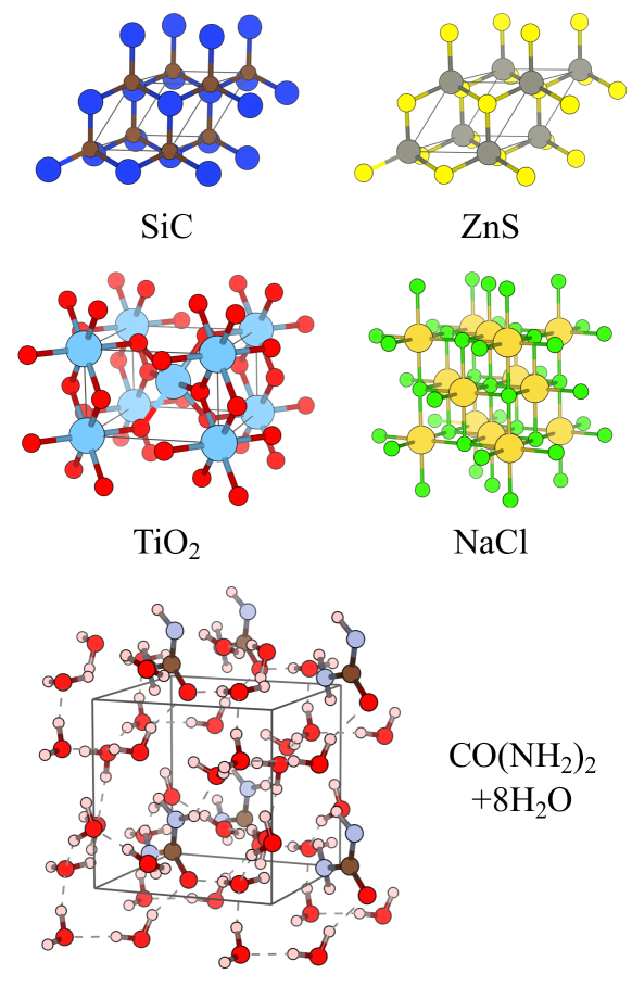
Figure 1: Structure of the systems tested in this work. The unit simulation cell is indicated by the grey box in each case.

III Computational details

We implemented all the estimators derived in Sections II.2 and II.3 as well as Algorithms 1 and 2 for calculating the periodic two-center and three-center SR ERIs in the PySCF software package Sun et al. (2018). We checked the correctness of our implementation by verifying that the calculated periodic integrals match those from the analytic Fourier transform (AFT) approach Sun et al. (2017) for small systems (limited by the high computational cost of AFT). The cutoff equations (48), (53), and (54) are solved numerically using a binary search algorithm. The bin size $\Delta d$ for grouping the bra AO pairs is set to be $1$ Å. All cutoffs and important cell (pair) data, including $\{R_{ab}^{\mathrm{cut}}\}$ and $\{\mathcal{M}_{a}\}$ for the two-center integrals (Section II.5.1) and $\{d_{ab}^{\mathrm{cut}}\}$, $\{R_{abc}^{\mathrm{cut}}(d_{ab}^{(i)})\}$, and $\{\mathcal{S}_{ab}^{(i)}\}$ for the three-center integrals (Section II.5.2), are precomputed and kept in memory before performing the lattice sum by Algorithms 1 and 2. The cost of the precomputation is in general only a small fraction of the subsequent lattice sum (up to a few percent in the worst cases).

Table 1: The exponent of the most diffuse orbital of given angular momentum for all basis sets used in this work. For each element, the first line is the AO basis, and the second line is the corresponding auxiliary basis ("JK" for the JKFIT basis and "ET" for the even tempered basis).

Element	Basis	$l$
		$0$	$1$	$2$	$3$	$4$	$5$	$6$
H	DZ	$0.122$	$0.727$
	JK	$0.284$	$0.502$	$0.713$
C	DZ	$0.160$	$0.152$	$0.550$
	JK	$0.192$	$0.203$	$0.200$	$0.416$
N	DZ	$0.225$	$0.218$	$0.817$
	JK	$0.273$	$0.282$	$0.290$	$0.609$
O	DZ	$0.302$	$0.275$	$1.185$
	JK	$0.339$	$0.367$	$0.356$	$0.825$
Na	DZ	$0.023$	$0.021$	$0.097$
	ET	$0.046$	$0.044$	$0.041$	$0.089$	$0.195$
Si	DZ	$0.092$	$0.088$	$0.275$
	JK	$0.132$	$0.185$	$0.170$	$0.237$
S	DZ	$0.157$	$0.141$	$0.479$
	JK	$0.216$	$0.263$	$0.242$	$0.396$
Cl	DZ	$0.194$	$0.162$	$0.600$
	JK	$0.234$	$0.306$	$0.275$	$0.499$
Ti	DZ	$0.025$	$0.029$	$0.052$	$0.279$
	ET	$0.051$	$0.055$	$0.059$	$0.078$	$0.104$	$0.241$	$0.558$
Zn	DZ	$0.038$	$0.046$	$0.252$	$1.462$
	ET	$0.075$	$0.084$	$0.093$	$0.216$	$0.503$	$1.213$	$2.923$
Zn	TZ	$0.038$	$0.046$	$0.252$	$1.485$	$4.114$
	ET	$0.075$	$0.084$	$0.093$	$0.216$	$0.503$	$1.223$	$2.970$
Zn	QZ	$0.037$	$0.039$	$0.159$	$0.853$	$2.069$	$4.414$
	ET	$0.074$	$0.076$	$0.078$	$0.157$	$0.319$	$0.737$	$1.706$

We assess both the accuracy of the estimators and the computational cost of the lattice sum based on them over a test set of four three-dimensional solids and a water-solvated urea molecule as shown in Fig. 1 (Cartesian coordinates in Supporting Information). The Dunning’s cc-pVXZ basis set Dunning (1989); Woon and Dunning (1993); Balabanov and Peterson (2005, 2006); Prascher et al. (2011) (abbreviated as "XZ" henceforth) is chosen as the AO basis. Specifically, we consider DZ for all systems and also TZ and QZ for ZnS. The cc-pVXZ-JKFIT basis set Weigend (2002) is used as the auxiliary basis for all elements except for Na, Ti, and Zn, for which the JKFIT basis set is not defined and we use the even tempered basis functions generated by PySCF with a progression factor $\beta=2.0$ (details in Supporting Information). The exponents of the most diffuse orbitals of all basis sets used in this work are summarized in Table 1. A series of $\omega$ values ranging from $0.1$ to $1$ are tested, which cover both the value used by the HSE functional ($\omega=0.11$) and those commonly used by the range-separated Gaussian density fitting Ye and Berkelbach (2021) (RSGDF). These choices (atom types, crystal structures, basis sets, and $\omega$ values) together make the numerical study of this work cover a wide range of parameters.

We measure the accuracy of the estimators in two ways. First, we calculate the intrinsic bra-ket cutoffs, $\{\tilde{R}_{ab}^{\mathrm{cut}}\}$ for the two-center case and $\{\tilde{R}_{abc}^{\mathrm{cut}}(d_{ab}^{(i)})\}$ for the three-center case, by solving Eq. 48 and Eq. 54 without the $f$-prefactor using both the exact SR ERIs and our estimators [the orbital orientation effect in the exact $\mathcal{J}_{abc}(\bm{R},\bm{d})$ is accounted for by averaging over three randomly generated configurations for each $(R,d)$]. The error of the estimated cutoffs then reflects directly the accuracy and tightness of the corresponding estimators. Second, we calculate the maximum absolute error (MAE) of the periodic SR ERI tensor, $[\mathbf{L}]_{ab}$ and $[\mathbf{L}]_{abc}$, computed using Algorithms 1 and 2 based on our estimators. This provides an indirect but more practical measure of the accuracy of the estimators for their applications to periodic systems.

Ideally, the error should be computed against the exact periodic integrals from the infinite lattice sum, which is unfortunately not possible in practice. To that end, we truncate the lattice sum using the most accurate estimators ($O_{l}v_{l}$ and ME for two- and three-center integrals, respectively, justified by the numerical data in Section IV) with a tight target precision of $\epsilon=10^{-12}$, and then perform the lattice sum without any screening, i.e., with the “if” statements in Algorithms 1 and 2 always set to true. For three-center integrals, this essentially amounts to using only the rigorous upper bound provided by the Schwarz inequality to discard unimportant AO pairs. We verified that internal consistency is achieved in all cases: the MAEs calculated as above are essentially the same as those calculated against the integrals obtained with $\epsilon=10^{-12}$ and with the screening based on the same estimator.

The computational cost is measured by either the number of integrals being evaluated (i.e., the number of times where the “if” statements in Algorithms 1 and 2 are evaluated to true) or the actual CPU time spent on the lattice sum. In this work, we will focus on the cost of the three-center integrals alone because the cost of evaluating the two-center integrals is essentially negligible in our applications.

IV Results and discussions

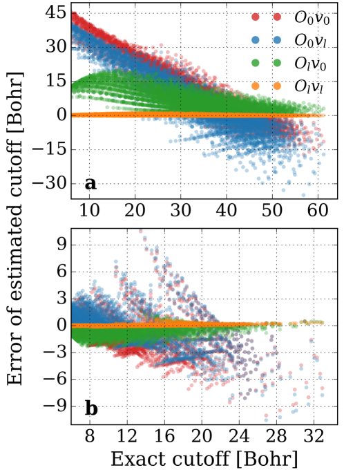
Figure 2: Error of the cutoffs for two-center SR ERIs estimated by the four estimators from Section II.2 with $\epsilon=10^{-10}$ plotted against the exact cutoffs for TiO2/DZ and two values of $\omega$, $0.1$ (a) and $1$ (b).

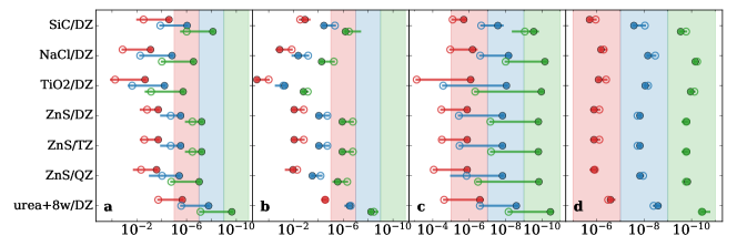
Figure 3: MAE of periodic two-center SR ERIs computed using Algorithm 1 with four different two-center estimators for integral screening: $O_{0}v_{0}$ (a), $O_{0}v_{l}$ (b), $O_{l}v_{0}$ (c), and $O_{l}v_{l}$ (d). Different colors are for different target precision, $\epsilon=10^{-6}$ (red), $10^{-8}$ (blue), and $10^{-10}$ (green), and the shaded area highlights $0.1\epsilon\sim 10\epsilon$ for the corresponding color. For each system and target precision, the horizontal bar shows the distribution of the MAEs for $\omega=0.1,0.2,\cdots,1$, where $\omega=0.1$ and $1$ are highlighted as a filled and hollow circles, respectively.

IV.1 Accuracy of two-center estimators

We first study the accuracy of the four two-center estimators from Section II.2. In Fig. 2, we show the error of the estimated cutoffs for TiO2/DZ with $\epsilon=10^{-10}$ for $\omega=0.1$ (a) and $\omega=1$ (b); the same plots for other systems are shown in Fig. S4. An immediate conclusion one can draw from these plots is that the $O_{l}v_{l}$ estimator (19) is very tight, predicting essentially the exact cutoffs in all cases. As a result, the periodic integrals $[\mathbf{L}]_{ab}$ computed based on the $O_{l}v_{l}$ estimator display highly controlled accuracy for all systems and all values of $\omega\in[0.1,1]$, as shown in Fig. 3(d). The high accuracy of the $O_{l}v_{l}$ estimator is due to the correct treatment of the $l$-dependence in both the orbital multipoles and the effective potential: ignoring the $l$-dependence in either or both cases generally leads to higher errors as can be seen in Fig. 2 (red, blue and green dots) and Fig. 3(a)–(c). These results can be understood as follows.

The $l$-dependence in the orbital multipoles depends strongly on the orbital exponents as $\zeta^{-(l+3/2)}$ [Eq. 20]. For diffuse orbitals ($\zeta\ll 1$) of high angular momentum, approximating $O_{l}$ by $O_{0}$ leads to significant underestimation. This explains the negative errors of the $O_{0}v_{0}$ (red) and the $O_{0}v_{l}$ (blue) estimators in Fig. 2 when the exact cutoffs are large, which produce large errors in the corresponding periodic integrals in Fig. 3(a) and (b). Also, the highest error of the periodic integrals is seen in TiO2 in both cases, because the even tempered auxiliary basis for Ti/DZ has very diffuse shells ($\zeta\lessapprox 0.1$) up to $l=4$ (Table 1). On the other hand, for non-$s$-type compact orbitals ($\zeta>1$), the $O_{0}$ approximation overestimates the true integrals as is clear from the large positive cutoff errors of the two $O_{0}$ estimators (red and blue) in Fig. 2 when the exact cutoffs are small. This does no harm to the accuracy of the periodic integrals over these orbitals but increases the computational cost.

The $l$-dependence in the effective potential shows a strong $\omega$-dependence. For $\omega$ small, the SR Coulomb potential resembles the full Coulomb potential, and approximating $v_{l}$ by $v_{0}$ overestimates the integrals as in the classical multipole interaction and leads to positive errors for the $O_{l}v_{0}$ estimator (green) in Fig. 2(a). This also explains two trends observed for the filled circles ($\omega=0.1$) in Fig. 3: (i) $O_{0}v_{0}$ is more accurate than $O_{0}v_{l}$ [Fig. 3(a) and (b)], and (ii) $O_{l}v_{0}$ is as accurate as $O_{l}v_{l}$ [Fig. 3(c) and (d)]. As $\omega$ increases, however, the $l$-dependence in $v_{l}$ starts to deviate from that of the classical multipole interaction and the $v_{0}$ approximation tends to underestimate the integrals. Consequently, negative errors are seen for the cutoffs of the $O_{l}v_{0}$ estimator (green) in Fig. 2(b) and quick growth of the MAEs of $[\mathbf{L}]_{ab}$ with $\omega$ is observed for the $O_{0}v_{0}$ and the $O_{l}v_{0}$ estimators in Fig. 3(a) and (c) (hollow circles), respectively.

To summarize the results for two-center estimators, the numerical data presented in Figs. 2 and 3 confirm the tightness of the $O_{l}v_{l}$ estimator and the accuracy of the resulting periodic integrals, hence justifying its use in Section II.3 for obtaining the three-center estimators, whose performance is discussed in the next section.

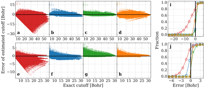
Figure 4: Error of the cutoffs for three-center SR ERIs estimated by the four estimators from Section II.3, ISF (a,e), ISF$Q_{0}$ (b,f), ISF$Q_{l}$ (c,g), and ME (d,h), with $\epsilon=10^{-10}$ plotted against the exact cutoffs for TiO2/DZ and two values of $\omega$, $0.1$ (a – d) and $1$ (e – h). Panels (i) and (j) show the fraction of estimated cutoffs with error lower than the abscissa.

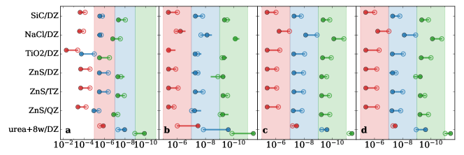
Figure 5: Same plot as Fig. 3 for the MAE of periodic three-center SR ERIs computed using Algorithm 2 with different three-center estimators for integral screening: ISF (a), ISF$Q_{0}$ (b), ISF$Q_{l}$ (c), and ME (d).

IV.2 Accuracy of three-center estimators

In Fig. 4, we show the error of the cutoffs computed by the four three-center estimators from Section II.3 for TiO2/DZ with $\epsilon=10^{-10}$ and $\omega=0.1$ and $1$; the same plots for other systems can be found in Figs. S5 and S6. An immediate conclusion from these plots is that the ISF estimator (28) significantly underestimates the true integrals in all cases. For TiO2, it underestimates about 80% of the cutoffs as shown in Fig. 4(i) and (j) (red circles). The underestimation by the ISF estimator comes from ignoring the higher-order multipoles of the bra AO product and results for TiO2 clearly show more severe underestimation for largelr $l_{ab}$ (Fig. S7). As a result, the MAEs of the periodic three-center SR ERIs computed based on the ISF estimator are two to four order of magnitude higher than the target precision as shown in Fig. 5(a). One exception is the solvated urea molecule, where the low packing density makes the $f$-prefactor (59) overestimate the truncation error, which cancels the underestimation by the ISF estimator and leads to MAEs $\lessapprox 10\epsilon$ in this case. In general, one should not rely on such fortuitous error cancellation.

The underestimation by the ISF estimator is largely corrected by the three other estimators that account for the higher-order multipoles of the bra AO product, as can be seen in Fig. 4(b)–(d) and (f)–(h). As expected from the discussion in Section II.3.3, the ISF$Q_{l}$ estimator (36) reduces essentially to the ISF$Q_{0}$ estimator (35) for small $\omega$ [Fig. 4(b) and (c)], but corrects the slight underestimation of the latter for large $\omega$ [Fig. 4(f) and (g)]. The ME estimator (41), which includes all terms in the multipole expansion with approximate GPT coefficients (39) and (42), is the most accurate among the three for large $\omega$ [Fig. 4(h)], but shows slight underestimation for small $\omega$ [Fig. 4(d)]. Overall, the three estimators have similar performance, and the difference between them is at most modest. This is also reflected by the high accuracy of the periodic integrals computed based on these estimators as shown in Fig. 5(b)–(d), where the MAEs typically fall in the range of $0.1\epsilon\sim 10\epsilon$ (with the solvated urea the only exception where the MAE is lower than $\epsilon$ for the reason discussed above).

In summary, the data in Figs. 4 and 5 suggest that ISF$Q_{0}$, ISF$Q_{l}$, and ME are all accurate estimators for three-center SR ERIs. In the next section, we will assess them based on the computational cost of the screened lattice sum.

IV.3 Computational cost of the lattice sum for three-center integrals

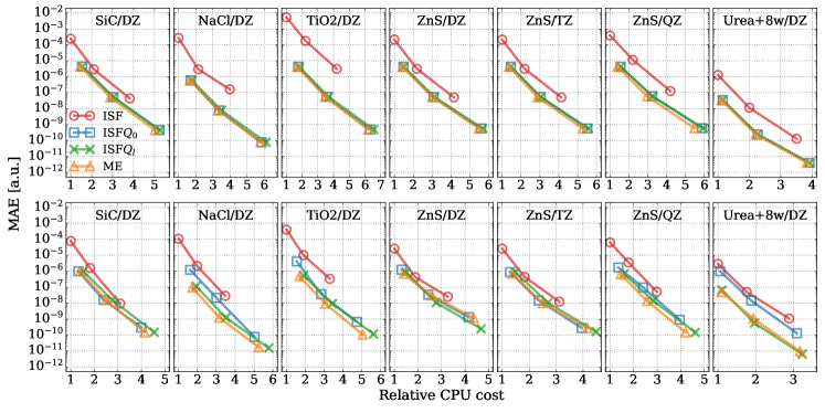
Figure 6: The MAE data taken from Fig. 5 plotted as a function of the CPU cost measured by the total number of integrals being calculated in the lattice sum (relative to the cost of ISF/$\epsilon=10^{-6}$) for $\omega=0.1$ (upper panels) and $1$ (lower panels).

IV.3.1 Computational efficiency

The results of the previous section clearly show increasing accuracy of the three-center estimator as its complexity grows. However, this alone does not justify the practical use of the more accurate estimators (ISF$Q_{0}$, ISF$Q_{l}$, and ME) because, although tedious, one can always empirically adjust the $\epsilon$ parameter for an inaccurate estimator (ISF in this case) to achieve the same accuracy for a specific system. We thus need to compare the computational cost of the lattice sum based on different estimators for achieving the same accuracy. We measure the computational cost by counting the number of integrals being evaluated in the lattice sum for computing the entire $[\mathbf{L}]_{abc}$ tensor and study its relation to the MAE data presented in Fig. 5.

The results are plotted in Fig. 6 for the two extreme cases, $\omega=0.1$ and $1$. In both cases, the ISF curves of all systems lie to the upper right of the curves of the other three estimators, suggesting consistently higher computational cost of the lattice sum based on the ISF estimator for achieving the same accuracy as the other three. For small $\omega$ (upper panels in Fig. 6), the saving in computational cost by using the more accurate estimators is as large as a factor of two in the most challenging case (TiO2). For large $\omega$ (lower panels in Fig. 6), however, only the ME estimator maintains the large saving against ISF for all systems, while the ISF$Q_{0}$ and ISF$Q_{l}$ curves both move closer to the ISF curve in some cases, indicating a loss of computational efficiency of the two Schwarz-$Q$ integral-based estimators for large $\omega$. This observation confirms that the ME estimator is tighter than the ISF$Q_{0}$ and ISF$Q_{l}$ estimators when $\omega$ is large.

IV.3.2 Scaling with $\omega$

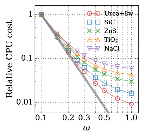
Figure 7: Relative CPU cost of the lattice sum for computing $[\mathbf{L}]_{abc}$ based on the ME estimator [Eq. 41] with $\epsilon=10^{-8}$ plotted as a function of $\omega$ (in log-log scale) for the five test systems in the DZ basis. The grey line indicates a perfect $\omega^{-3}$ scaling of the relative CPU cost.

We next investigate how the cost of the screened lattice sum scales with $\omega$. Given that the characteristic decay length of the SR Coulomb potential is roughly $\omega^{-1}$, one may expect $\omega^{-3}$ scaling for three-dimensional systems. However, as discussed in Section II.2, the decay of the final SR ERIs is described instead by an effective potential, $v_{l}(\eta,R)$ [Eq. 21], where the bare $\omega$ is replaced, for three-center integrals, by $\eta_{abc\omega}$ [Eq. 29], which depends not only on $\omega$ but also on the exponents of the orbitals. This means that different elements in the $[\mathbf{L}]_{abc}$ tensor need different computational effort, and the term with the smallest $\eta_{abc\omega}$ represents the computational bottleneck. The smallest $\eta_{abc\omega}$ (call it $\eta_{abc\omega}^{\mathrm{min}}$) for a given system is roughly the minimum of $\omega^{2}$ and half the smallest AO exponent, $\eta_{\mathrm{AO}}^{\mathrm{min}}\equiv\zeta_{\mathrm{AO}}^{\mathrm{min}}/2$.

We predict the following two limits for the scaling of the computational cost with $\omega$. In the small $\omega$ regime where $\omega\ll[\eta_{\mathrm{AO}}^{\mathrm{min}}]^{1/2}$, we have $\eta_{abc\omega}^{\mathrm{min}}\approx\omega^{2}$ and we expect the ideal $\omega^{-3}$ scaling. In the large $\omega$ regime where $\omega\gg[\eta_{\mathrm{AO}}^{\mathrm{min}}]^{1/2}$, we have $\eta_{abc\omega}^{\mathrm{min}}\approx\eta_{\mathrm{AO}}^{\mathrm{min}}$ and we expect a plateau in the cost as a function of $\omega$. These asymptotic predictions are confirmed numerically in Fig. 7 for the ME estimator with $\epsilon=10^{-8}$; other choices of the estimator and $\epsilon$ lead to essentially identical plots (Fig. S8). In all cases, the cost follows the ideal $\omega^{-3}$ decay (grey line) but then begins to plateau as $\omega$ increases. The crossover point between these asymptotic behaviors (and therefore also the plateau height) are consistent with the values of $[\eta_{\mathrm{AO}}^{\mathrm{min}}]^{1/2}$ for these systems: $0.25$ for the solvated urea, $0.21$ for SiC, $0.14$ for ZnS, $0.11$ for TiO2, and $0.10$ for NaCl (all calculated using the data from Table 1).

IV.3.3 Scaling with system size

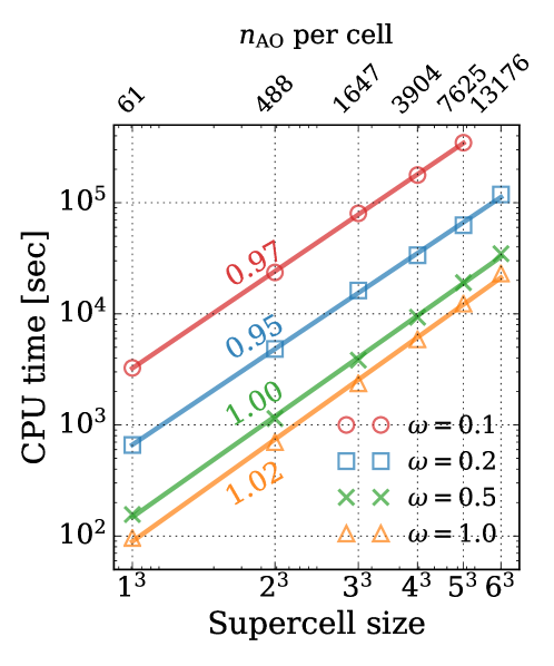
Figure 8: CPU time for the lattice sum for computing $[\mathbf{L}]_{abc}$ using the ME estimator with $\epsilon=10^{-8}$ for ZnS/DZ of different supercell size and different values of $\omega$. Each line is a linear fit for the data of the same color. The apparent scaling factors obtained from the fitting are listed aside, all showing linear scaling with system size. The number of AOs per supercell is also shown in the top abscissa.

In periodic calculations, an infinite system is approximated by a finite simulation supercell subject to Born-von Karman periodic boundary conditions (Section II.5). This introduces a finite-size error that must be removed by increasing the size of the simulation supercell (or equivalently the density of Brillouin zone sampling). Gygi and Baldereschi (1986); Paier et al. (2006); Spencer and Alavi (2008); Broqvist, Alkauskas, and Pasquarello (2009); Guidon, Hutter, and VandeVondele (2009); Sundararaman and Arias (2013); Azadi and Foulkes (2015); McClain et al. (2017) Therefore, in this final section, we study how the cost of the screened lattice sum scales with the size of the supercell.

For each element of the $[\mathbf{L}]_{abc}$ tensor, the number of integrals that pass the screening is $\sum_{i}^{n_{d_{ab}}}|\mathcal{S}_{abc}^{(i)}|$, where $\mathcal{S}_{abc}^{(i)}$ is defined in Eq. 55. Thus, the total computational cost for executing Algorithm 2 is proportional to

$$N_{\mathrm{I}}=\sum_{a,b}^{n_{\mathrm{AO}}}\sum_{i}^{n_{d_{ab}}}\sum_{c}^{n_{\mathrm{aux}}}|\mathcal{S}_{abc}^{(i)}|,$$ (61)

where both $n_{\mathrm{AO}}$ and $n_{\mathrm{aux}}$ grow linearly with the system size while $\{n_{d_{ab}}\}$ remain constant, which seems to suggest cubic scaling with system size. However, since the cutoffs, $\{d_{ab}^{\mathrm{cut}}\}$ [Eq. 53] and $\{R_{abc}^{\mathrm{cut}}\}$ [Eq. 54], depend only on the nature of the orbitals and are independent of the system size, we expect a quadratic decrease of the number of elements in each $\mathcal{S}_{abc}^{(i)}$ with system size according to Eq. 55. This suggests that the overall scaling with system size is linear if integral screening is performed as described in Section II.5.2.

To confirm this analysis, we perform a series of supercell calculations for ZnS/DZ. A supercell of size $n_{\mathrm{p}}^{3}$ is constructed by repeating a primitive cell $n_{\mathrm{p}}$ times in each of the three dimensions. The CPU time of the lattice sum for computing the entire $[\mathbf{L}]_{abc}$ tensor using the ME estimator with $\epsilon=10^{-8}$ is shown in Fig. 8 for $n_{\mathrm{p}}=1-6$ and four different values of $\omega$. Results generated using the ISF$Q_{0}$ and the ISF$Q_{l}$ estimators show similar trends (Fig. S9). For all choices of $\omega$, the results demonstrate nearly perfect linear scaling with the supercell size.

V Concluding remarks

In summary, we derived distance-dependent estimators for the two-center and three-center SR ERIs over atom-centered GTOs. Performance was assessed by the accuracy of the periodic two-center and three-center SR ERIs, which are calculated using the estimators to screen the integrals appearing in the lattice summation. Based on the numerical data collected for systems that cover a wide range of parameters including the atom types, crystal structures, orbital exponents and angular momenta, and the range-separation parameter $\omega$, we recommend the $O_{l}v_{l}$ estimator (19) and the ME estimator (41) for two-center and three-center SR ERIs, respectively. In the case of small $\omega$ (such as that used in the HSE functional), the ISF$Q_{0}$ estimator (35) is also a good choice for three-center SR ERIs. We discussed why the computational scaling of the lattice sum for three-center integrals deviates from $\omega^{-3}$, and show that the cost scales linearly with system size for all tested values of $\omega$.

Although we chose to demonstrate their use for periodic systems, the estimators derived in this work also should be useful in large molecular applications. We also expect our results to be useful for semiempirical methods, where two-center and three-center ERIs are typical, and phenomenologically screened or otherwise SR Coulomb interactions are commonly used. For ab initio periodic calculations using our recently developed range-separated Gaussian density fitting Ye and Berkelbach (2021) (RSGDF), building the three-center SR ERI tensor represents one of the main computational bottlenecks–at least for Hartree-Fock and lower-order perturbation theory. We thus anticipate the estimators together with the algorithms for screening the lattice sum to improve the computational efficiency of such calculations.

Supplementary material

See the supplementary material for (i) the performance of ME estimator (41) for three-center SR ERIs with concentric bra pairs (i.e., $d_{ab}=0$), (ii) the effect of using different $f$-prefactors to solve Eq. 48 on the performance of the $O_{l}v_{l}$ estimator, (iii) the error of the estimated two-center cutoffs, (iv) the error of the estimated three-center cutoffs, (v) AO angular momentum-resolved error plot of the estiamted three-center cutoffs, (vi) the CPU cost of the lattice sum for computing $[\mathbf{L}]_{abc}$ plotted as a function of $\omega$ for different choices of estimator and $\epsilon$, (vii) the CPU time of the lattice sum for computing $[\mathbf{L}]_{abc}$ plotted as a function of the supercell size of ZnS/DZ for the ISF$Q_{0}$ and the ISF$Q_{l}$ estimators, (viii) Cartesian coordinates of the test systems shown in Fig. 1, (ix) details of the even tempered basis functions for Na, Ti, and Zn.

Appendix A Fourier transform of primitive GTOs and SR Coulomb potentials

$$\begin{split}\tilde{\phi}_{alm}(\bm{q})&=\int\mathrm{d}\bm{r}\,\mathrm{e}^{-\mathrm{i}\bm{q}\cdot\bm{r}}\phi_{alm}(\bm{r})\\ &=\mathrm{i}^{l}(\pi/\zeta_{a})^{3/2}(2\zeta_{a})^{-l}q^{l}\mathrm{e}^{-q^{2}/(4\zeta_{a})}y_{lm}(\hat{\bm{q}})\end{split}$$ (62)

$$\tilde{g}_{\omega}(\bm{q})=\int\mathrm{d}\bm{r}\,\mathrm{e}^{-\mathrm{i}\bm{q}\cdot\bm{r}}g_{\omega}(\bm{r})=\frac{4\pi}{q^{2}}\big{(}1-\mathrm{e}^{-q^{2}/(4\omega^{2})}\big{)}$$ (63)

Appendix B Asymptotic analysis of Eq. 14

The integral (14) can be analytically performed,

$$I(R;L,l,\eta)=2^{L-1}\pi^{1/2}\frac{\Gamma(\alpha)}{\Gamma(\beta)}\eta^{\alpha}R^{\beta-3/2}M(\alpha,\beta;-\eta R^{2})$$ (64)

where $\alpha=(L+l+1)/2$, $\beta=l+3/2$, and $M(a,b;z)$ is the confluent hypergeometric function of the first kind. Using the asymptotic behavior of $M(a,b;z)$ at large $|z|$,

$$M(a,b;z)\sim\Gamma(b)\bigg{[}\frac{\mathrm{e}^{z}z^{a-b}}{\Gamma(a)}+\frac{(-z)^{-a}}{\Gamma(b-a)}\bigg{]},$$ (65)

we obtain an asymptotic expression for Eq. 64 at large $R$,

$$I(R;L,l,\eta)\sim 2^{L-1}\pi^{1/2}\bigg{[}\frac{\Gamma(\alpha)}{\Gamma(\beta-\alpha)R^{L+1}}-R^{L-2}\eta^{L-1/2}\mathrm{e}^{-\eta R^{2}}\bigg{]}.$$ (66)

The first term decaying as $R^{L+1}$ is the long-range classical multipole interaction. As this term is $\eta$-independent, its contribution to Eq. 12 vanishes when taking the difference. The second term decaying exponentially with $R$ is the short-range interaction via orbital overlap. Its contribution to Eq. 12 is non-vanishing but $l$-independent.

Data availability statement

The data that support the findings of this study are available from the corresponding author upon reasonable request.

References

- White et al. (1994) C. A. White, B. G. Johnson, P. M. Gill, and M. Head-Gordon, Chem. Phys. Lett. 230, 8 (1994).
- Strout and Scuseria (1995) D. L. Strout and G. E. Scuseria, J. Chem. Phys. 102, 8448 (1995).
- White et al. (1996) C. A. White, B. G. Johnson, P. M. Gill, and M. Head-Gordon, Chem. Phys. Lett. 253, 268 (1996).
- White and Head-Gordon (1996) C. A. White and M. Head-Gordon, J. Chem. Phys. 105, 5061 (1996).
- Strain, Scuseria, and Frisch (1996) M. C. Strain, G. E. Scuseria, and M. J. Frisch, Science 271, 51 (1996).
- Challacombe, Schwegler, and Almlöf (1996) M. Challacombe, E. Schwegler, and J. Almlöf, J. Chem. Phys. 104, 4685 (1996).
- Schwegler and Challacombe (1996) E. Schwegler and M. Challacombe, J. Chem. Phys. 105, 2726 (1996).
- Challacombe and Schwegler (1997) M. Challacombe and E. Schwegler, J. Chem. Phys. 106, 5526 (1997).
- Ochsenfeld, White, and Head-Gordon (1998) C. Ochsenfeld, C. A. White, and M. Head-Gordon, J. Chem. Phys. 109, 1663 (1998).
- Schütz, Lindh, and Werner (1999) M. Schütz, R. Lindh, and H.-J. Werner, Mol. Phys. 96, 719 (1999).
- Lambrecht, Doser, and Ochsenfeld (2005) D. S. Lambrecht, B. Doser, and C. Ochsenfeld, J. Chem. Phys. 123, 184102 (2005).
- Doser et al. (2009) B. Doser, D. S. Lambrecht, J. Kussmann, and C. Ochsenfeld, J. Chem. Phys. 130, 064107 (2009).
- Maurer et al. (2013) S. A. Maurer, D. S. Lambrecht, J. Kussmann, and C. Ochsenfeld, J. Chem. Phys. 138, 014101 (2013).
- Dyczmons (1973) V. Dyczmons, Theor. Chim. Acta 28, 307 (1973).
- Häser and Ahlrichs (1989) M. Häser and R. Ahlrichs, J. Comput. Chem. 10, 104 (1989).
- Gill, Johnson, and Pople (1994) P. M. Gill, B. G. Johnson, and J. A. Pople, Chem. Phys. Lett. 217, 65 (1994).
- Maurer et al. (2012) S. A. Maurer, D. S. Lambrecht, D. Flaig, and C. Ochsenfeld, J. Chem. Phys. 136, 144107 (2012).
- Hollman, Schaefer, and Valeev (2015) D. S. Hollman, H. F. Schaefer, and E. F. Valeev, J. Chem. Phys. 142, 154106 (2015).
- Valeev and Shiozaki (2020) E. F. Valeev and T. Shiozaki, J. Chem. Phys. 153, 097101 (2020).
- Peels and Knizia (2020) M. Peels and G. Knizia, J. Chem. Theory Comput. 16, 2570 (2020).
- Whitten (1973) J. L. Whitten, J. Chem. Phys. 58, 4496 (1973).
- Dunlap, Connolly, and Sabin (1979) B. I. Dunlap, J. W. D. Connolly, and J. R. Sabin, J. Chem. Phys. 71, 3396 (1979).
- Mintmire and Dunlap (1982) J. W. Mintmire and B. I. Dunlap, Phys. Rev. A 25, 88 (1982).
- Savin and Flad (1995) A. Savin and H.-J. Flad, Int. J. Quantum Chem. 56, 327 (1995).
- Leininger et al. (1997) T. Leininger, H. Stoll, H.-J. Werner, and A. Savin, Chem. Phys. Lett. 275, 151 (1997).
- Adamson, Dombroski, and Gill (1999) R. D. Adamson, J. P. Dombroski, and P. M. W. Gill, J. Comput. Chem. 20, 921 (1999).
- Iikura et al. (2001) H. Iikura, T. Tsuneda, T. Yanai, and K. Hirao, J. Chem. Phys. 115, 3540 (2001).
- Heyd, Scuseria, and Ernzerhof (2003) J. Heyd, G. E. Scuseria, and M. Ernzerhof, J. Chem. Phys. 118, 8207 (2003).
- Toulouse, Colonna, and Savin (2004) J. Toulouse, F. Colonna, and A. Savin, Phys. Rev. A 70, 062505 (2004).
- Yanai, Tew, and Handy (2004) T. Yanai, D. P. Tew, and N. C. Handy, Chem. Phys. Lett. 393, 51 (2004).
- Refaely-Abramson et al. (2013) S. Refaely-Abramson, S. Sharifzadeh, M. Jain, R. Baer, J. B. Neaton, and L. Kronik, Phys. Rev. B 88, 081204 (2013).
- Lutsker, Aradi, and Niehaus (2015) V. Lutsker, B. Aradi, and T. A. Niehaus, J. Chem. Phys. 143, 184107 (2015).
- Jung et al. (2005) Y. Jung, A. Sodt, P. M. W. Gill, and M. Head-Gordon, Proc. Natl. Acad. Sci. 102, 6692 (2005).
- Reine et al. (2008) S. Reine, E. Tellgren, A. Krapp, T. Kjærgaard, T. Helgaker, B. Jansik, S. Høst, and P. Salek, J. Chem. Phys. 129, 104101 (2008).
- Heyd, Scuseria, and Ernzerhof (2006) J. Heyd, G. E. Scuseria, and M. Ernzerhof, J. Chem. Phys. 124, 219906 (2006).
- Izmaylov, Scuseria, and Frisch (2006) A. F. Izmaylov, G. E. Scuseria, and M. J. Frisch, J. Chem. Phys. 125, 104103 (2006).
- Guidon et al. (2008) M. Guidon, F. Schiffmann, J. Hutter, and J. VandeVondele, J. Chem. Phys. 128, 214104 (2008).
- Guidon, Hutter, and VandeVondele (2009) M. Guidon, J. Hutter, and J. VandeVondele, J. Chem. Theory Comput. 5, 3010 (2009).
- Shang, Li, and Yang (2011) H. Shang, Z. Li, and J. Yang, J. Chem. Phys. 135, 034110 (2011).
- Beuerle, Kussmann, and Ochsenfeld (2017) M. Beuerle, J. Kussmann, and C. Ochsenfeld, J. Chem. Phys. 146, 144108 (2017).
- Ye and Berkelbach (2021) H.-Z. Ye and T. C. Berkelbach, J. Chem. Phys. 154, 131104 (2021).
- Schlegel and Frisch (1995) H. B. Schlegel and M. J. Frisch, Int. J. Quantum Chem. 54, 83 (1995).
- Boys (1950) S. F. Boys, Proc. Roy. Soc. Lond. A 200, 542 (1950).
- Szabo and Ostlund (1996) A. Szabo and N. S. Ostlund, Modern Quantum Chemistry: Introduction to Advanced Electronic Structure Theory (Dover Publications Inc., Mineola, New York, 1996).
- Besalú (2011) C.-D. R. Besalú, E., J. Math. Chem. 49, 1769 (2011).
- Fermann and Valeev (2020) J. T. Fermann and E. F. Valeev, “Fundamentals of molecular integrals evaluation,” (2020), arXiv:2007.12057v1 .
- Matsuoka (1998a) O. Matsuoka, J. Mol. Struct.: THEOCHEM 451, 35 (1998a).
- Matsuoka (1998b) O. Matsuoka, J. Chem. Phys. 108, 1063 (1998b).
- Sun et al. (2018) Q. Sun, T. C. Berkelbach, N. S. Blunt, G. H. Booth, S. Guo, Z. Li, J. Liu, J. D. McClain, E. R. Sayfutyarova, S. Sharma, S. Wouters, and G. K.-L. Chan, Wiley Interdiscip. Rev. Comput. Mol. Sci 8, e1340 (2018).
- Sun et al. (2017) Q. Sun, T. C. Berkelbach, J. D. McClain, and G. K.-L. Chan, J. Chem. Phys. 147, 164119 (2017).
- Dunning (1989) T. H. Dunning, J. Chem. Phys. 90, 1007 (1989).
- Woon and Dunning (1993) D. E. Woon and T. H. Dunning, J. Chem. Phys. 98, 1358 (1993).
- Balabanov and Peterson (2005) N. B. Balabanov and K. A. Peterson, J. Chem. Phys. 123, 064107 (2005).
- Balabanov and Peterson (2006) N. B. Balabanov and K. A. Peterson, J. Chem. Phys. 125, 074110 (2006).
- Prascher et al. (2011) B. P. Prascher, D. E. Woon, K. A. Peterson, T. H. Dunning, and A. K. Wilson, Theor. Chem. Acc. 128, 69 (2011).
- Weigend (2002) F. Weigend, Phys. Chem. Chem. Phys. 4, 4285 (2002).
- Gygi and Baldereschi (1986) F. Gygi and A. Baldereschi, Phys. Rev. B 34, 4405 (1986).
- Paier et al. (2006) J. Paier, M. Marsman, K. Hummer, G. Kresse, I. C. Gerber, and J. G. Ángyán, J. Chem. Phys. 124, 154709 (2006).
- Spencer and Alavi (2008) J. Spencer and A. Alavi, Phys. Rev. B 77, 193110 (2008).
- Broqvist, Alkauskas, and Pasquarello (2009) P. Broqvist, A. Alkauskas, and A. Pasquarello, Phys. Rev. B 80, 085114 (2009).
- Sundararaman and Arias (2013) R. Sundararaman and T. A. Arias, Phys. Rev. B 87, 165122 (2013).
- Azadi and Foulkes (2015) S. Azadi and W. M. C. Foulkes, J. Chem. Phys. 143, 102807 (2015).
- McClain et al. (2017) J. McClain, Q. Sun, G. K.-L. Chan, and T. C. Berkelbach, J. Chem. Theory Comput. 13, 1209 (2017).