Approximation Theory of Convolutional Architectures for Time Series Modelling

Abstract

We study the approximation properties of convolutional architectures applied to time series modelling, which can be formulated mathematically as a functional approximation problem. In the recurrent setting, recent results reveal an intricate connection between approximation efficiency and memory structures in the data generation process. In this paper, we derive parallel results for convolutional architectures, with WaveNet being a prime example. Our results reveal that in this new setting, approximation efficiency is not only characterised by memory, but also additional fine structures in the target relationship. This leads to a novel definition of spectrum-based regularity that measures the complexity of temporal relationships under the convolutional approximation scheme. These analyses provide a foundation to understand the differences between architectural choices for time series modelling and can give theoretically grounded guidance for practical applications.

1 Introduction

While deep learning has evolved to be a powerful tool to model temporal relationships, the choice of architectures significantly affects performance. Classical recurrent neural networks (RNNs) and recent adaptation of convolutional neural networks (CNNs) to time series data represent two popular classes of architectural choices. Empirical works show that depending on the application setting, either one can have an advantage over the other (Yin et al., 2017; Bai et al., 2018; Banerjee et al., 2019). However, a concrete theoretical understanding of how such differences arise remains largely unexplored.

The recent work of Li et al. (2021) formulated the temporal modelling task into a functional analysis problem, and uncovered relationships between approximation efficiency of RNNs and memory structures of the target relationship. In this paper, we develop parallel results for CNNs in the functional approximation setting. On the one hand, these results provide approximation guarantees and rate estimations for CNNs applied to time series modelling. On the other hand, they allow us to concretely understand the differences between CNNs and RNNs in terms of their approximation capabilities for temporal relationships, serving as a starting point to bridge theories and applications.

Our main contributions are:

1. We develop universal approximation results for CNNs when applied to model temporal relationships in the linear setting, which shows that the approximation efficiency is characterised by both memory structures and a certain spectrum-based regularity of the target relationship.

2. We make rigorous comparisons between CNNs and RNNs in the approximation setting, where we show that the targets that can be easily approximated are completely different for these two architectures. This provides a theoretical foundation for building principled model selection strategies for deep learning in dynamical settings.

The paper is organised as follows. We discuss related work in Section 2. In Section 3, we formulate the approximation problem precisely and introduce the RNN and CNN hypothesis spaces under this formulation. The approximation results of CNNs are presented in Section 4. In Section 5, we make a concrete comparison between CNNs and RNNs in terms of approximation capabilities for different classes of target temporal relationships. The proofs of all presented results are found in the appendix.

1.1 Notations and definitions.

We use boldface letters $\bm{x}$ to denote discrete temporal sequences, and $x(t)$ to denote the vector/scalar value of the sequence at the time index $t$. We use $\bm{x}_{[t_{1},t_{2}]}$ to denote values of the sequence $\bm{x}$ from $t_{1}$ to $t_{2}$, including the end points. Subscripts such as $\bm{x}_{i}$, $\bm{x}_{m}$ are used to specify dimensional indices. All other dependencies are written as superscripts, e.g. $\bm{x}^{(K)}$ means that the temporal sequence $\bm{x}$ depends on $K$. For a discrete sequence $\bm{\rho}:\mathbb{N}\to\mathbb{R}^{d}$, define the radius of $\bm{\rho}$ by $r(\bm{\rho})=\sup\left\{s:\rho(s)\neq 0\right\}$. We refer $[0,r(\bm{\rho})]$ as its support. We use $\lvert\cdot\rvert$ to denote the Euclidean norm of a vector.

We set the notation for the central operation under study, namely the dilated convolution for discrete sequences.

Definition 1.

Let $\bm{f}:\mathbb{Z}\to\mathbb{R}^{d}$, $\bm{g}:\mathbb{Z}\to\mathbb{R}^{d}$ be two discrete sequences. Define the following discrete dilated convolution:

$$(\bm{f}\mathop{\scalebox{1.7}{\raisebox{-0.86108pt}{$\ast$}}}{}_{l}\,\bm{g})(t)=\sum_{s\in\mathbb{Z}}f(s)^{\top}g(t-ls).$$ (1)

When $l=1$, this is the usual convolution, and we denote it by $\mathop{\scalebox{1.7}{\raisebox{-0.86108pt}{$\ast$}}}$.

2 Related work

In this section, we discuss some related work to the results presented here. On the application side, convolution-based models are gradually becoming popular for a variety of time series applications. For example, WaveNet (van den Oord et al., 2016) is a generative model for processing and generating raw audio. Since its emergence, WaveNet and its variants (van den Oord et al., 2018; Jin et al., 2018; Kalchbrenner et al., 2018; Prenger et al., 2019; Paine et al., 2016) have been successfully applied to a variety of time series modelling problems in natural language processing. A more detailed review can be found in Boilard et al. (2019). While convolutional architectures have become an important alternative to classical recurrent neural networks, these investigations focus on applications, lacking theoretical results to understand the origin of their superior performance on practical tasks.

On the theoretical side, a number of universal approximation results for CNNs have been obtained in the image processing setting. For example, Zhou (2020a, b) prove that (simplified) deep CNNs are universal approximators, and the approximation rate is characterised by Sobolev norms of target functions. Bao et al. (2019) gives a theoretical interpretation on the reason why the state-of-the-art CNNs can achieve high classification accuracy. It is shown that the hierarchical compositional structures in target functions can help to (exponentially) reduce the parameters needed compared with fully connected neural networks achieving the same approximation accuracy. Beyond the approximation theory, Oono & Suzuki (2019) studies the estimation error rates of a ResNet-type of CNN applied to the Barron and Hölder classes. All of these works share one thing in common, namely the targets to be approximated are functions defined in finite space domains, i.e. images. By contrast, our approximation results here are for the targets defined in infinite time domains, where the memory of data plays an important role. We will see that this leads to very different approximation problems.

On the recurrent front, the approximation properties of RNNs have been investigated in a number of works, including both in discrete time (Matthews, 1993; Doya, 1993; Schäfer & Zimmermann, 2006, 2007) and continuous time (Funahashi & Nakamura, 1993; Chow & Xiao-Dong Li, 2000; Li et al., 2005; Maass et al., 2007; Nakamura & Nakagawa, 2009). Most of these study settings where the target relationships are generated from hidden dynamical systems (in the form of difference or differential equations). Recently, Li et al. (2021) studies the general setting where the target relationships are represented as functionals, and derived the approximation theory of RNNs that revealed the connection between approximation and memory: it takes an exponentially large number of neurons to approximate the target with memory that decays slowly. This sheds some light on the interaction of the structure of RNNs and the nature of relationships to be captured. Following this line of enquiry, the purpose of the present paper is to develop parallel approximation results for CNNs to highlight such interactions. In particular, this work complements previous theoretical analyses in the recurrent setting and allows one to characterise the key difference between recurrent and convolutional approaches for time series modelling.

3 Problem Formulation

3.1 Functional formulation of supervised learning for temporal data

The temporal supervised learning task can be mathematically formulated as follows. Suppose we are given an input sequence $\bm{x}$ indexed by a time parameter $t\in\mathbb{Z}$. We want to predict the corresponding output sequence $\bm{y}$ at each time step, or up to some terminal time step $y(T)$. The mapping between $\bm{x}$ and $\bm{y}$ can be described by a sequence of functionals:

$$\left\{y(t)=H_{t}(\bm{x}):t\in\mathbb{Z}\right\}.$$ (2)

That is, the output at each time step may potentially depend on the entire input sequence through a time-dependent functional. The goal is to learn this sequence of functionals $\bm{H}=\left\{H_{t}:t\in\mathbb{Z}\right\}$.

As an illustrative example, we can consider a standard benchmark example known as the adding problem (Hochreiter & Schmidhuber, 1997): each output $y(t)$ is equal to the weighted cumulative sum of inputs $x(s)$ for $s\leq t$, i.e. $y(t)=\sum_{-\infty}^{t}\alpha(s)x(s)$, where $\alpha$ denotes the weights. In this case, the sequence of functionals $\{H_{t}(\bm{x})=\sum_{-\infty}^{t}\alpha(s)x(s):t\in\mathbb{Z}\}$ can be viewed as the target temporal relationship, or ground truth.

In supervised learning, we need to define the input space, output space and concept space precisely. We note that vector-valued discrete temporal sequences can also be understood as functions from a time index set $\mathcal{I}$ into the real vectors. We denote this set of functions by $\bm{c}(\mathcal{I},\mathbb{R}^{d})$. In this paper, $\mathcal{I}$ is taken to be $\mathbb{Z}$ or $\mathbb{N}$ depending on the specific setting. For $\bm{x}\in\bm{c}(\mathcal{I},\mathbb{R}^{d})$, we define its norm by $\lVert\bm{x}\rVert_{2}:=\sqrt{\sum_{s\in\mathcal{I}}\lvert x(s)\rvert^{2}}$. We use $\bm{c}_{0}(\mathbb{N},\mathbb{R}^{d})$ to denote the sequence that converges to 0 at infinity.

Define the input space by

$$\mathcal{X}=\Big{\{}\bm{x}\in\bm{c}(\mathbb{Z},\mathbb{R}^{d}):\sum_{s\in\mathbb{Z}}\lvert x(s)\rvert^{2}<\infty\Big{\}}.$$ (3)

This is the usual $\ell^{2}$ sequence space, which is a Banach space with the norm $\lVert\bm{x}\rVert_{\mathcal{X}}:=\lVert\bm{x}\rVert_{2}=\sqrt{\sum_{s\in\mathbb{Z}}\lvert x(s)\rvert^{2}}$.

Since vector-valued outputs can be handled by considering each dimension individually, we can restrict our attention to the case where the output time series are real-valued. That is, define the output space

$$\mathcal{Y}=\bm{c}(\mathbb{Z},\mathbb{R}).$$ (4)

3.2 RNN and CNN hypothesis spaces

We now introduce the RNN and CNN architectures in the functional approximation language, which leads to different types of hypothesis spaces. We start with the recurrent setting. The simplest recurrent neural network with the linear readout layer is given by

$$h{(t+1)} =\sigma(Wh(t)+Ux(t)),$$ (5)

$$\hat{y}(t) =c^{\top}h(t),$$

$$\text{with }c\in\mathbb{R}^{m},W \in\mathbb{R}^{m\times m},U\in\mathbb{R}^{m\times d}.$$

Here, $h\in\mathbb{R}^{m}$ is the hidden state and $m$ denotes the width of RNNs, which determines the model complexity. Note that we do not include a bias term here because it can be absorbed into the hidden state $h$.

This dynamics defines a family of functionals

$$\mathcal{H}_{\text{RNN}}^{(m)}:= \Big{\{}\bm{\hat{H}}:\hat{H}_{t}=\hat{y}(t)\text{ solves (\ref{eq: rnndynamics}) }$$ (6)

$$~{}~{}\text{with }\text{$c\in\mathbb{R}^{m}$},\text{$W\in\mathbb{R}^{m\times m}$, $U\in\mathbb{R}^{m\times d}$}\Big{\}}.$$

The hypothesis space for one layer RNNs with arbitrary depth is defined by

$$\mathcal{H}_{\text{RNN}}:=\bigcup_{m\in\mathbb{N}_{+}}\mathcal{H}_{\text{RNN}}^{(m)}.$$ (7)

In essence, RNNs can be understood as a way to represent functionals by introducing hidden dynamical systems, with the predicted outputs being observations.

Recent approaches based on convolutional architectures present an entirely different class of methods to parameterise the functionals. Concretely, a convolution based temporal sequence model with $K$ layers and $M_{k}$ channels at layer $k$ is given by

$$\bm{h}_{0,i} =\bm{x}_{i},$$ (8)

$$\bm{h}_{k+1,i} =\sigma\left(\sum_{j=1}^{M_{k}}{\bm{w}}_{kji}\mathop{\scalebox{1.7}{\raisebox{-0.86108pt}{$\ast$}}}{}_{d_{k}}\bm{h}_{k,j}\right),$$

$$\bm{\hat{y}} =\bm{h}_{K}.$$

Here, $\bm{x}_{i}$ is the $i^{th}$ dimension of $\bm{x}$, and ${\bm{w}}_{kji}$ is the filter from channel $j$ at layer $k$ to the channel $i$ at layer $k+1$. All the filters have a size $l\geq 2$, i.e. $r({\bm{w}}_{kji})=l\geq 2$. In the following discussion, we assume that the dilation rate satisfies $d_{k}=l^{k}$. That is, the dilation rate increases exponentially for each layer to achieve an exponentially large receptive field. This is the standard practice for dilated convolutional structures (Oord et al., 2016; Yu & Koltun, 2016).

The CNN model (8) also defines a family of functionals

$${{\mathcal{H}}}_{\text{CNN}}^{(l,K,\left\{M_{k}\right\})}:= \Big{\{}\bm{\hat{H}}:\hat{H}_{t}=\hat{y}(t)\text{ according to \eqref{eq: CNNdynamics}}$$ (9)

$$~{}~{}\text{with $\bm{w}_{kji}\in\mathbb{R}^{l}$}\Big{\}}.$$

For any $l\geq 2$ and $d_{k}=l^{k}$, the hypothesis space for CNNs with arbitrary depth and number of channels is defined as

$${{\mathcal{H}}}_{\text{CNN}}^{(l)}=\bigcup_{K\in\mathbb{N}_{+}}\bigcup_{\left\{M_{k}\right\}\in\mathbb{N}_{+}^{K}}{{\mathcal{H}}}_{\text{CNN}}^{(l,K,\left\{M_{k}\right\})}.$$ (10)

4 Approximation theory for convolutional structures

In this section, we study the approximation properties of ${{\mathcal{H}}}_{\text{CNN}}^{(l)}$. Our main results consist of two parts. First, we prove that ${{\mathcal{H}}}_{\text{CNN}}^{(l)}$ is dense in appropriate concept spaces. Next, we derive explicit upper and lower bounds for the approximation rate, which depends on the depth and width of CNNs, together with appropriate notions of complexity of the target functional family. This is an important result that characterises the kind of targets that can be well-approximated by CNNs using a small number of parameters.

To make analysis amenable, we consider the linear setting. This is non-trivial for two reasons: first, the key feature we would like to study for time series applications is the dependence on time, for which non-linearity still plays an important role even in the case of linear activations. For example, we will see that the Riesz representation of a linear functional is nonlinear in time. The approximation results for RNNs (Li et al., 2021) has already demonstrated this. Second, since the approximation results for linear RNNs have been derived in Li et al. (2021), by adopting the same setting we can study explicitly the differences between RNNs and CNNs. Under the assumption that the activation $\sigma$ is linear, the RNN and CNN hypothesis spaces can be further simplified as

$$\mathcal{H}_{\text{RNN}}^{(m)}:= \Big{\{}\bm{\hat{H}}:\hat{H}_{t}(\bm{x})=\sum_{s\in\mathbb{N}}c^{\top}W^{s-1}Ux(t-s),$$ (11)

$$~{}~{}\text{$c\in\mathbb{R}^{m},W\in\mathbb{R}^{m\times m}$, $U\in\mathbb{R}^{m\times d}$}\Big{\}},$$

$${{\mathcal{H}}}_{\text{CNN}}^{(l,K,\left\{M_{k}\right\})}:= \Big{\{}\bm{\hat{H}}:\hat{H}_{t}(\bm{x})=\sum_{s\in\mathbb{N}}\rho^{(\bm{\hat{H}})}(s)^{\top}x(t-s),$$ (12)

$$\bm{\rho}^{(\bm{\hat{H}})}(s)=\sum_{i_{K-1}=1}^{M_{K-1}}\bm{w}_{K-1,i_{K-1},t}\mathop{\scalebox{1.7}{\raisebox{-0.86108pt}{$\ast$}}}{}_{l^{K-1}}$$

$$\sum_{i_{K-2}=1}^{M_{K-2}}\bm{w}_{K-2,i_{K-2},i_{K-1}}\mathop{\scalebox{1.7}{\raisebox{-0.86108pt}{$\ast$}}}{}_{l^{K-2}}$$

$$\cdots\mathop{\scalebox{1.7}{\raisebox{-0.86108pt}{$\ast$}}}{}_{l^{2}}\sum_{i_{1}=1}^{M_{1}}\bm{w}_{1i_{1}i_{2}}\mathop{\scalebox{1.7}{\raisebox{-0.86108pt}{$\ast$}}}{}_{l^{1}}\bm{w}_{0i_{1}}(s)\Big{\}}.$$

We will also restrict to a target functional family (concept space) that is consistent with the linear activation setting. The following definition is introduced in Li et al. (2021).

Definition 2.

Let $\bm{H}=\left\{H_{t}:t\in\mathbb{Z}\right\}$ be a sequence of functionals which satisfies

1. $\bm{H}$ is causal if it does not depend on the future inputs: for any $\bm{x}_{1},\bm{x}_{2}\in\mathcal{X}$ and any $t\in\mathbb{Z}$ such that $x_{1}(s)=x_{2}(s)\ \text{ for all }s\leq t$, the output satisfies $H_{t}(\bm{x}_{1})=H_{t}(\bm{x}_{2})$;

2. $H_{t}\in\bm{H}$ is a continuous linear functional if for any $\bm{x}_{1},\bm{x}_{2}\in\mathcal{X}$ and $\lambda_{1},\lambda_{2}\in\mathbb{R}$,

   $$\begin{gathered}H_{t}(\lambda_{1}\bm{x}_{1}+\lambda_{2}\bm{x}_{2})=\lambda_{1}H_{t}(\bm{x}_{1})+\lambda_{2}H_{t}(\bm{x}_{2}),\\ \lVert H_{t}\rVert:=\sup_{\bm{x}\in\mathcal{X},\lVert\bm{x}\rVert_{\mathcal{X}}\leq 1}\lvert H_{t}(\bm{x})\rvert<\infty,\end{gathered}$$ (13)

   where $\lVert H_{t}\rVert$ denotes the induced functional norm. Furthermore, the norm of a sequence of functionals is defined by $\lVert\bm{H}\rVert:=\sup_{t\in\mathbb{Z}}\lVert H_{t}\rVert$.

3. A sequence of functionals $\bm{H}$ is time-homogeneous if for any $t,\tau\in\mathbb{Z}$, $H_{t}(\bm{x})=H_{t+\tau}(\bm{x}^{(\tau)})$ where $x^{(\tau)}(s):=x(s-\tau)$ for all $s\in\mathbb{Z}$.

Following the Definition 2, we consider the concept space

$$\mathcal{C}= \{\bm{H}:\text{ $H_{t}\in\bm{H}$ is linear continuous, $\bm{H}$}$$ (14)

$$~{}~{}\text{ is causal and time-homogeneous}\}.$$

Note that $\mathcal{H}_{\text{RNN}}\subset\mathcal{C}$ and ${{\mathcal{H}}}_{\text{CNN}}^{(l)}\subset\mathcal{C}$, which follows from the fact that any sequences in these two spaces have convolutional (thus linear) representations. For a given $\bm{\hat{H}}$, we denote its corresponding representation by $\bm{\rho}^{(\bm{\hat{H}})}$. We see that RNNs and CNNs are different in the sense that for RNNs, the representation $\rho^{(\bm{\hat{H}})}(s)=c^{\top}W^{s-1}U$, which has an infinite support in time. However, for CNNs, the representation $\bm{\rho}^{(\bm{\hat{H}})}$ is a finitely supported sequence with radius $r(\bm{\rho}^{(\bm{\hat{H}})})=l^{K}-1$. This can be understood as the maximal memory length of the CNN model, which is usually called the receptive field.

Next we present a key lemma regarding the hypothesis space, which shows that any target in the concept space has a convolutional representation.

Lemma 1.

For any $\bm{H}\in\mathcal{C}$, there exists a unique $\ell^{2}$ sequence $\bm{\rho}^{(\bm{H})}:\mathbb{N}\to\mathbb{R}^{d}$ such that

$$H_{t}(\bm{x})=\sum_{s=0}^{\infty}\rho^{(\bm{H})}(s)^{\top}x(t-s),\quad t\in\mathbb{Z}.$$ (15)

For a target $\bm{H}$, the corresponding representation is denoted as $\bm{\rho}^{(\bm{H})}$. The approximation of $\bm{H}$ by RNNs or CNNs is equivalent to the approximation of $\bm{\rho}^{(\bm{H})}$ using the respective $\bm{\rho}^{(\bm{\hat{H}})}$.

Remark 1.

The hypothesis space is related with linear time-invariant system (LTI system). In fact, a causal LTI system will induce a linear functional which satisfies Definition 2. However, we note that not every linear functional satisfying Definition 2 corresponds to an LTI system. Our aim is to investigate general funtionals, and does not assume the data is generated from a hidden linear system.

4.1 Summary of approximation results for RNNs

In order to facilitate the presentation of CNN results and subsequent comparisons, we first review the main approximation results for RNNs proved in Li et al. (2021) . It was shown that under fairly general conditions, $\mathcal{H}_{\text{RNN}}$ is dense in $\mathcal{C}$. With further assumptions that $\bm{\rho}^{(\bm{H})}$ decays at least exponentially in time, an explicit bound of the approximation rate can be obtained. That is, for any $\bm{H}\in\mathcal{C}$, there exists $\bm{\hat{H}}\in\mathcal{H}_{\text{RNN}}^{(m)}$ such that

$$\lVert\bm{H}-\bm{\hat{H}}\rVert\equiv\sup_{t\in\mathbb{R}}\lVert H_{t}-\hat{H}_{t}\rVert\leq\frac{C\gamma d}{\beta m^{\alpha}},$$ (16)

where $C>0$ is a universal constant, $\beta$ denotes the (exponential) decay rate of $\bm{\rho}^{(\bm{H})}$ and $\gamma$ measures the smoothness of $\bm{H}$. This result shows that a target functional family generating the temporal relationship can be well approximated by RNN models if it is smooth and decays sufficiently fast. For a target with long memory, say a power law decay, the number of parameters sufficient to approximate it using RNNs may increase exponentially. This is the so-called “curse of memory” in approximation of RNNs (Li et al., 2021).

4.2 Approximation results for CNNs

In this section, we present the main approximation results of this paper, which can be viewed as parallel results to those discussed in section 4.1, but for CNNs. This allows us to understand precisely the similarity and differences of CNNs and RNNs with respect to their approximation capabilities, when applied to time series modelling.

First, we prove a density result. Recall that ${{\mathcal{H}}}_{\text{CNN}}^{(l)}\subset\mathcal{C}$. The density result here shows that ${{\mathcal{H}}}_{\text{CNN}}^{(l)}$ is in fact dense in $\mathcal{C}$. It is also understood as a universal approximation property of linear CNNs applied to linear functionals.

Theorem 2.

(UAP for CNNs) Let $\bm{H}\in\mathcal{C}$. Then for any $\epsilon>0$, there exist $\bm{\hat{H}}\in{{\mathcal{H}}}_{\text{CNN}}^{(l)}$ such that

$$\lVert\bm{H}-\bm{\hat{H}}\rVert\equiv\sup_{t\in\mathbb{Z}}\lVert H_{t}-\widehat{H}_{t}\rVert<\epsilon.$$ (17)

Now we discuss some basic understanding of Theorem 2. For any $\bm{x}$ such that $\lVert\bm{x}\rVert_{\mathcal{X}}\leq 1$, we have

$$\lvert H_{t}(\bm{x})-\hat{H}_{t}(\bm{x})\rvert^{2}\leq\sum_{s=0}^{\infty}\Big{\rvert}\bm{\rho}^{(\bm{H})}(s)-\bm{\rho}^{(\bm{\hat{H}})}(s)\Big{\rvert}^{2}$$ (18)

$$=\sum_{s=0}^{l^{K}-1}\Big{\rvert}\bm{\rho}^{(\bm{H})}(s)-\bm{\rho}^{(\bm{\hat{H}})}(s)\Big{\rvert}^{2}+\sum_{s=l^{K}}^{\infty}\Big{\rvert}\bm{\rho}^{(\bm{H})}(s)\Big{\rvert}^{2},$$

where we use the fact that $r(\bm{\rho}^{(\bm{\hat{H}})})=l^{K}-1$. Consider the approximation error on two intervals. On $[l^{K},\infty]$, $\bm{\rho}^{(\bm{\hat{H}})}$ is always zero, thus the error only depends on the tail sum of $\bm{\rho}^{(\bm{H})}$. That is, the long term memory of the target. Since $\bm{\rho}^{(\bm{H})}\in\ell^{2}$, this error converges to zero when we choose a deep model (with $K$ appropriately large). On $[0,l^{K}-1]$, we can show that there exits a $\bm{\rho}^{(\bm{\hat{H}})}$ with a sufficient number of channels such that $\bm{\rho}^{(\bm{\hat{H}})}=\bm{\rho}^{(\bm{H})}$ in this range.

The error on $[l^{K},\infty]$ is easy to analyse as it only involves the decay of $\bm{\rho}^{(\bm{H})}$, which enters in the approximation of both RNNs and CNNs. The more interesting phenomenon occurs on the interval $[0,l^{K}-1]$. A natural question is, given a target $\bm{H}$, how does the approximation error on this interval depend on the number of channels and depth of CNNs? This question is important since it reveals the structures in the target functional family which facilitate efficient approximation using CNNs besides the decay of memory. In other words, it characterises theoretically the type of temporal modelling tasks for which CNNs are naturally suited.

Interestingly, it turns out that the approximation rate depends on the spectrum of $\bm{\rho}^{(\bm{H})}$ under a suitable tensorisation procedure. We motivate this idea by simple examples where $d=1$ and $l=K=2$.

Example 1.

Recall that a target $\bm{H}$ has the representation $\bm{\rho}^{(\bm{H})}$. Since $r(\bm{\rho}^{(\bm{\hat{H}})})=4$ here, the CNN performs approximation only on $[0,3]$, hence we restrict the target as $\bm{\rho}^{(\bm{H})}_{[0,3]}\in\mathbb{R}^{4}$. Denote the rearrangement operator by $T$, and

$$T\Big{(}\bm{\rho}^{(\bm{H})}_{[0,3]}\Big{)}=\begin{pmatrix}\rho^{(\bm{H})}_{0}&\rho^{(\bm{H})}_{2}\\ \rho^{(\bm{H})}_{1}&\rho^{(\bm{H})}_{3}\end{pmatrix}.$$ (19)

We study the singular value decomposition (SVD) of the matrix $T\Big{(}\bm{\rho}^{(\bm{H})}_{[0,3]}\Big{)}$. If $T\Big{(}\bm{\rho}^{(\bm{H})}_{[0,3]}\Big{)}$ has only one non-zero singular value, then $\mathrm{rank}~{}T\Big{(}\bm{\rho}^{(\bm{H})}_{[0,3]}\Big{)}=1$. It is straightforward to deduce that a CNN with 1 channel in both layers is sufficient to represent it. In fact, let $\bm{w}_{1}$ and $\bm{w}_{2}$ be the filter on the first and second layer respectively. The resulting representation is

$$\bm{\rho}^{(\bm{\hat{H}})}=\bm{w}_{2}\mathop{\scalebox{1.7}{\raisebox{-0.86108pt}{$\ast$}}}{}_{2}\,\bm{w}_{1} =(w_{11},w_{12})\mathop{\scalebox{1.7}{\raisebox{-0.86108pt}{$\ast$}}}{}_{2}(w_{21},w_{22})$$ (20)

$$=(w_{11}w_{21},w_{12}w_{21},w_{11}w_{22},w_{12}w_{22}),$$

$$T(\bm{\rho}^{(\bm{\hat{H}})}) =\begin{pmatrix}w_{11}w_{21}&w_{11}w_{22}\\ w_{12}w_{21}&w_{12}w_{22}\end{pmatrix}$$ (21)

$$=\begin{pmatrix}w_{11}\\ w_{12}\end{pmatrix}\begin{pmatrix}w_{21}&w_{22}\end{pmatrix}.$$ (22)

This can represent any 2 by 2 rank 1 matrix. Thus, any $\bm{\rho}^{(\bm{H})}$ such that $T\big{(}\bm{\rho}^{(\bm{H})}_{[0,3]}\big{)}$ with rank no more than 1 can be represented.

In order to represent a rank 2 target, we need to increase the number of channels. Let the first layer have $2$ channels. Then the resulting representation is

$$\begin{gathered}\bm{\rho}^{(\bm{\hat{H}})}=\bm{w}_{2}\mathop{\scalebox{1.7}{\raisebox{-0.86108pt}{$\ast$}}}{}_{2}\,\bm{w}_{1}+\bm{v}_{2}\mathop{\scalebox{1.7}{\raisebox{-0.86108pt}{$\ast$}}}{}_{2}\,\bm{v}_{1},\\ T(\bm{\rho}^{(\bm{\hat{H}})})=\begin{pmatrix}w_{11}w_{21}&w_{11}w_{22}\\ w_{12}w_{21}&w_{12}w_{22}\end{pmatrix}+\begin{pmatrix}v_{11}v_{21}&v_{11}v_{22}\\ v_{12}v_{21}&v_{12}v_{22}\end{pmatrix}\\ =\begin{pmatrix}\frac{1}{\sqrt{\sigma}_{1}}w_{11}&\frac{1}{\sqrt{\sigma}_{2}}v_{11}\\ \frac{1}{\sqrt{\sigma}_{1}}w_{12}&\frac{1}{\sqrt{\sigma}_{2}}v_{12}\end{pmatrix}\begin{pmatrix}\sigma_{1}&\\ &\sigma_{2}\end{pmatrix}\begin{pmatrix}\frac{1}{\sqrt{\sigma}_{1}}w_{21}&\frac{1}{\sqrt{\sigma}_{2}}v_{21}\\ \frac{1}{\sqrt{\sigma}_{1}}w_{22}&\frac{1}{\sqrt{\sigma}_{2}}v_{22}\end{pmatrix}^{\top}.\end{gathered}$$ (23)

That is, $T(\bm{\rho}^{(\bm{\hat{H}})})$ can represent the SVD for any 2 by 2 matrix with appropriate choices of $\bm{w}_{1},\bm{w}_{2}$ and $\bm{v}_{1}$, which implies that $T\big{(}\bm{\rho}^{(\bm{H})}_{[0,3]}\big{)}$ with rank no more than 2 can be represented.

The above two examples show that the number of channels needed for an exact representation ($\bm{\rho}^{(\bm{\hat{H}})}_{[0,3]}=\bm{\rho}^{(\bm{H})}_{[0,3]}$) depends on the rank of targets, i.e. the number of non-zero singular values of $T\big{(}\bm{\rho}^{(\bm{H})}_{[0,3]}\big{)}$. Furthermore, when there is no such exact representations, we need to decide the approximation error. Suppose the target is with rank 2, but we use a CNN with only $1$ channel to approximate it. By the Eckart–Young–Mirsky theorem, the best approximation error is equal to the smallest singular value of $T\big{(}\bm{\rho}^{(\bm{H})}_{[0,3]}\big{)}$. This inspires us to relate the approximation error with the decay of singular values.

The above examples illustrate the basic approach on how to determine the number of channels needed to achieve a given approximation accuracy. Although the main tool used in above examples, SVD, is only valid for $K=2$ where we can reshape the vector representation of $\bm{\rho}^{(\bm{H})}$ into a matrix, in general we can extend the above techniques to any $K$ using higher order singular value decomposition (HOSVD) (De Lathauwer et al., 2000). Now we introduce some basic facts about HOSVD.

HOSVD basics.

For a discrete sequence $\bm{\rho}$, we denote the tensorisation of $\bm{\rho}_{[0,l^{K}-1]}$ by $T_{l^{K}}(\bm{\rho})$. This is an order $K$ tensor, with all the dimensions equal to $l$ i.e. $T_{l^{K}}(\bm{\rho})\in\mathbb{R}^{l\times l\times\cdots\times l}$. The tensorisation follows column major ordering. The singular values of $T_{l^{K}}(\bm{\rho})$ is defined by applying the usual SVD for matrices to the $K$ matrices with size $\mathbb{R}^{l\times l^{K-1}}$ obtained by mode-$k$ flattening of the tensor. This gives rise to at most $lK$ singular values. Define the rank of the tensor by its number of non-zero singular values. We defer the precise but involved definition of HOSVD to the appendix.

Similar to the SVD low rank approximation for matrices, we have the following error estimation for tensors (De Lathauwer et al., 2000).

Lemma 3.

Denote the singular values of $\bm{\mathcal{A}}\in\mathbb{R}^{l\times l\times\cdots\times l}$ by $\sigma_{1}\geq\sigma_{2}\geq\cdots\geq\sigma_{lK}\geq 0$, we have

$$\inf_{\bm{\hat{H}}}\left\|\bm{\mathcal{A}}-T_{l^{K}}(\bm{\rho}^{(\bm{\hat{H}})})\right\|\leq\left(\sum_{i=K^{\prime}+1}^{\operatorname{rank}{\bm{\mathcal{A}}}}\sigma_{i}^{2}\right)^{\frac{1}{2}},$$ (24)

where the infimum is taken over all $\bm{\hat{H}}\in{{\mathcal{H}}}_{\text{CNN}}^{(l,K,\left\{M_{k}\right\})}$ such that $K^{\prime}<\operatorname{rank}\bm{\mathcal{A}}$, where $K^{\prime}=\operatorname{rank}{T_{l^{K}}(\bm{\rho}^{(\bm{\hat{H}})})}$.

Based on Lemma 3, one can measure the complexity of a target $\bm{H}$ by the decay rate of singular values of $T_{l^{K}}(\bm{\rho}^{(\bm{H})})$.

Complexity measure and approximation rates.

Now we can get down to define appropriate complexity measures and prove approximation rates of CNNs. Based on previous discussions on HOSVD, we have the following key definition.

Definition 3.

Consider a sequence of functionals $\bm{H}$ with associated representation $\bm{\rho}^{(\bm{H})}$. For any $l,K\in\mathbb{N}_{+}$, let $\sigma_{1}^{(K)}\geq\sigma_{2}^{(K)}\geq\cdots\geq\sigma_{lK}^{(K)}\geq 0$ be the singular values of $T_{l^{K}}(\bm{\rho}^{(\bm{H})})$. Let $g\in\bm{c}_{0}(\mathbb{N},\mathbb{R}_{+})$ be a non-increasing function with zero limit at infinity. Define the complexity measure of $\bm{H}$ by

$$C^{(l,g)}(\bm{H})=\inf\Bigg{\{}c:\left(\sum_{i=s+K}^{lK}\lvert\sigma_{i}^{(K)}\rvert^{2}\right)^{\frac{1}{2}}\leq cg(s),$$ (25)

$$~{}s\geq 0,K\geq 1\Bigg{\}}.$$

Based on this complexity measure, we define a concept space with certain spectral regularity (measured by the decay of singular values)

$$\mathcal{C}^{(l,g)}:=\left\{\bm{H}\in\mathcal{C}:C^{(l,g)}(\bm{H})<\infty\right\}.$$ (26)

Next, we discuss some facts and examples to enhance the understanding of the space $\mathcal{C}^{(l,g)}$.

Remark 2.

Suppose the function $g$ is monotonously decreasing and strictly positive. Then for any $\bm{H}\in\mathcal{C}$ such that $\bm{\rho}^{(\bm{H})}$ is finitely supported, we have $\bm{H}\in\mathcal{C}^{(l,g)}$.

Remark 3.

Suppose $\bm{H}\in\mathcal{C}$ with $\bm{\rho}^{(\bm{H})}$ finitely supported. Then there exists a finitely supported decreasing $g$ such that $\bm{H}\in\mathcal{C}^{(l,g)}$.

The details can be found in appendix.

The reason why the summation in (25) starts at $s+K$ is that, when $K$ increases, there will be additional singular values resulting from the additional matrix SVDs. These singular values are all equal to the 2-norm of $\bm{\rho}^{(\bm{H})}$. We show this by the following example.

Example 2.

Suppose the filter size $l=2$ and $\bm{\rho}^{(\bm{H})}=$ $(1,0,0,1,0,0,0,\cdots)$. The following table shows the corresponding singular values of $T_{l^{K}}(\bm{\rho}^{(\bm{H})})$ for different $K$:

K	Singular Values of $T_{l^{K}}(\bm{\rho}^{(\bm{H})})$
1	$(1,1)$
2	$(1,1,1,1)$
3	$(\sqrt{2},1,1,1,1,0)$
4	$(\sqrt{2},\sqrt{2},1,1,1,1,0,0)$

When $K\geq 2$, $[0,l^{K}-1]$ covers the support of $\bm{\rho}^{(\bm{H})}$. If we further increase $K$, there will be additional singular values all equal to $\lVert\bm{\rho}^{(\bm{H})}\rVert_{2}=\sqrt{2}$.

For $K\geq 2$, we have

$$\sum_{i=s+K}^{lK}\lvert\sigma_{i}^{(K)}\rvert^{2}=\begin{cases}2,&s=1\\ 1,&s=2.\\ 0,&\text{otherwise}\end{cases}$$ (27)

Then given $g$ one can compute $C^{(l,g)}(\bm{H})$ based on (25) and (27).

Based on Definition 3, we can now present our main result on the approximation rate of CNNs.

Theorem 4.

(Approximation rate for CNNs) Fix $l\geq 2$ and $g\in\bm{c}_{0}(\mathbb{N},\mathbb{R}_{+})$. For any $\bm{H}\in\mathcal{C}^{(l,g)}$ and any set of parameters $(K,\left\{M_{k}\right\})$, we have

$$\frac{1}{\sqrt{d}}\sup_{t\in[l^{K},\infty]}\lvert\bm{\rho}^{(\bm{H})}(t)\rvert\leq\inf_{\bm{\hat{H}}\in{{\mathcal{H}}}_{\text{CNN}}^{(l,K,\left\{M_{k}\right\})}}\lVert\bm{H}-\bm{\hat{H}}\rVert\leq$$ (28)

$$d\ g(KM^{\frac{1}{K}}-K)C^{(l,g)}(\bm{H})+{\lVert\bm{\rho}^{(\bm{H})}_{[l^{K},\infty]}\rVert_{2}},$$

where $M:=\frac{1}{d}(\sum_{k=2}^{K}M_{k}M_{k-1}-lK)$ denotes the effective number of filters.

As discussed earlier, the term $\lVert\bm{\rho}^{(\bm{H})}_{[l^{K},\infty]}\rVert_{2}$ is the error on $[l^{K},\infty]$, due to the limited support of depth-$K$ CNNs. This error can be reduced by increasing the number of layers $K$, and it is less important as $l^{K}$ increases exponentially fast.

Hence, the subsequent discussion will focus on the more interesting term, i.e. the approximation error on the interval $[0,l^{K}-1]$: $d\ g(KM^{\frac{1}{K}}-K)C^{(l,g)}(\bm{H})$. This is related to the complexity measure of $\bm{H}$, which is small if there exists effective low rank structures in the target. With the fact that $\operatorname{rank}{T_{l^{K}}(\bm{\rho}^{(\bm{\hat{H}})})}$ is at least $KM^{\frac{1}{K}}$ (see details in appendix), combining Lemma 3 and (25) gives the result. Given a target $\bm{H}$, this error can be reduced by either increasing the number of filters $M$ or the number of layers $K$.

Whether a target $\bm{H}$ can be easily approximated depends on $C^{(l,g)}(\bm{H})$, which is determined by the decay of singular values of $T_{l^{K}}(\bm{\rho}^{(\bm{H})})$. For $T_{l^{K}}(\bm{\rho}^{(\bm{H})})$ with fast decaying singular values, even if the rank is large or $\bm{\rho}^{(\bm{H})}$ decays slowly, one can still have a good approximation with CNNs. This is very different from previous results of RNNs.

We now introduce an example to illustrate this observation. Consider 3 targets with the following representations

$$\begin{gathered}\rho_{1}(t)=\begin{cases}\frac{\pi^{2}}{12},&t=17,18,25,26\\ 0,&\text{otherwise}\end{cases},\\ \rho_{2}(t)=\begin{cases}\frac{\pi^{2}}{12},&t=9,15,19,26\\ 0,&\text{otherwise}\end{cases},\ \ \rho_{3}(t)=\frac{1}{t}.\end{gathered}$$

Note that all of them are instances of the adding problem. Moreover, they all have the same magnitude, $\lVert\bm{\rho}_{1}\rVert_{2}=\lVert\bm{\rho}_{2}\rVert_{2}=\lVert\bm{\rho}_{3}\rVert_{2}$. The support of both $\bm{\rho}_{1},\bm{\rho}_{2}$ are finite, while $\bm{\rho}_{3}$ have an infinite support. Furthermore, $\bm{\rho}_{1}$ and $\bm{\rho}_{2}$ have the same number of non-zero entries. We plot the error bound of each targets in Figure 1.

First, from the figure we conclude that the approximation can be reduced by increasing $K$ or $M$. For a fixed $K$, when $M$ is sufficiently large such that the rank of the model is no less than the rank of the target, the error will no longer decrease if we further increase $M$. At this point the error only comes from the tail which can only be reduced by increasing $K$ (hence increasing the support, or receptive field of the CNN model).

Next, we compare $\bm{\rho_{1}}$ and $\bm{\rho_{2}}$. From Figure 1, we conclude that $\bm{\rho_{1}}$ is easier to approximate than $\bm{\rho_{2}}$. The only difference between these two targets is the position of their non-zero entries, which results in $T_{2^{5}}(\bm{\rho_{1}})$ being rank 5 while $T_{2^{5}}(\bm{\rho_{2}})$ being rank 10. This is the case where low rank structures facilitates the approximation by CNNs.

Finally, we make a comparison between $\bm{\rho_{2}}$ and $\bm{\rho_{3}}$. We conclude that $\bm{\rho_{3}}$ is easier to approximate as the overall error is smaller than $\bm{\rho_{2}}$, in spite of the fact that $\bm{\rho_{2}}$ is finitely supported and has a simple form. The reason is that the tail sum of singular values of $T_{l^{K}}(\bm{\rho_{3}})$ decays faster than that of $T_{l^{K}}(\bm{\rho}_{2})$. This illustrates the case where a target with fast decaying singular values (i.e. low effective rank) can be easily approximated.

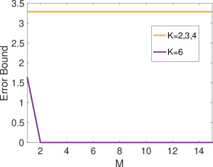
(a) $\bm{\rho}_{1}$

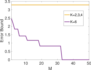
(b) $\bm{\rho}_{2}$

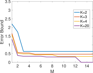
(c) $\bm{\rho}_{3}$

Figure 1: Let $l=2$. We plot the upper bound of the approximation errors against the effective number of filters. Each line corresponds to a fixed $K$. The error bound is calculated based on Theorem 4, where the tail term is calculated directly and the rank term is determined by numerically compute the singular values of $T_{l^{K}}(\bm{\rho}_{i})$. These curves describe, according to Theorem 4, the decay of approximation errors of CNNs as one increases the number of filters. Observe that the decay depends on the low rank structures of the targets.

5 Comparison of CNNs and RNNs in terms of approximation

As motivated earlier, how to judiciously choose architectures for time series modelling is an important practical problem, and prior works only address it empirically. Combining the approximation theory for CNNs developed here and those for RNNs in Li et al. (2021), we are in a position to provide theoretical answers to such problems, albeit in specific settings. This is the purpose of the present section.

In short, our theoretical analyses show that neither CNNs nor RNNs are always better than the other. Whether one out-performs its counterpart depends on the properties of the target relationship. Our results make this statement precise, and provide general guidelines on how to select architectures based on applications. We begin by presenting two representative examples for the two aforementioned cases, from which we can infer key differences between RNNs and CNNs for time series modelling.

Example where RNNs out-perform CNNs.

We assume a scalar input with $d=1$. Consider a target $\bm{H}\in\mathcal{C}$ with the representation $\rho^{\bm{H}}(t)=\gamma^{t}$, where $0<\gamma<1.$ It is easy for RNNs to approximate this target, since the representation has a power form. In fact, we have $\bm{H}\in\mathcal{H}_{\text{RNN}}^{(1)}$, i.e. a RNN with one hidden unit is sufficient to achieve an exact representation, with 0 approximation error for any $\gamma$.

For a CNN $\bm{\hat{H}}\in{{\mathcal{H}}}_{\text{CNN}}^{(l)}$, based on the lower bound of the approximation error from Theorem 4, we have that $\lVert\bm{H}-\bm{\hat{H}}\rVert^{2}\geq\sup_{t\in[l^{K},\infty]}\lVert\bm{\rho}^{(\bm{H})}(t)\rVert_{2}.$ Thus, in order to achieve an approximation error with $\lVert\bm{H}-\bm{\hat{H}}\rVert^{2}<\epsilon$, we have $\sup_{t\in[l^{K},\infty]}\lVert\bm{\rho}^{(\bm{H})}(t)\rVert_{2}=\gamma^{l^{K}}<\epsilon.$ This implies $l^{K}\geq\frac{\log(\epsilon)}{\log(\gamma)}$. That is to say, the necessary number of layers to achieve an approximation error smaller than $\epsilon$ diverges to infinity as $\gamma$ approaches 1.

Example where CNNs out-perform RNNs.

Still assume a scalar input with $d=1$. Consider a target $\bm{H}\in\mathcal{C}$ with representation $\rho^{(\bm{H})}(t)=\delta(t-2^{K})$ where $K\in\mathbb{N}_{+}$. This is an discrete time impulse at $t=2^{K}$ and can be regarded as the copying memory problem (Bai et al., 2018): given an input $\bm{x}$, the output $\bm{y}$ satisfies $y(t)=x(t-2^{K})$. We have $\bm{H}\in{{\mathcal{H}}}_{\text{CNN}}^{(2,K,\left\{1\right\})}$. Thus, a $K$-layer CNN with one channel per layer is sufficient to achieve an exact representation.

Recall that RNN approximates the target $\bm{\rho}^{(\bm{H})}$ with a power sum $\bm{\rho}^{(\bm{\hat{H}})}(s)=c^{\top}W^{s-1}U$. Suppose here $W\in\mathbb{R}^{m\times m}$ is a diagonalisable matrix with negative eigenvalues. The latter has a special structure, which makes it difficult to approximate certain functions. Suppose $u$ is a $m$-term power sum, i.e. $u(t)=c_{0}+\sum_{i=1}^{m}c_{i}\ \gamma_{i}^{t}.$ Then according to (Borwein & Erdélyi, 1996), we have

$$\lvert u(t+1)-u(t)\rvert\leq\frac{2m}{t}\sup_{s\geq 0}u(s).$$ (29)

For a fixed number of terms $m$, the changes between $u(t+1)$ and $u(t)$ approaches zero as $t$ approaches infinity. This means that if there is a sudden change in $u$ far from origin, the number of terms $n$ must be large.

For a RNN $\bm{\hat{H}}\in\mathcal{H}_{\text{RNN}}^{(m)}$, assume $\lVert\bm{H}-\bm{\hat{H}}\rVert<\epsilon.$ Let $u(s)=c^{\top}W^{s-1}U$ denote the power sum corresponding to $\bm{\hat{H}}$. Since $W$ is a $m\times m$ matrix, $u(s)$ is a $m^{2}$-term power sum. We have that $\lvert u(2^{K}+1)-u(2^{K})\rvert>1-2\epsilon,$ and hence (29) implies $m^{2}>2^{K-1}\frac{1-2\epsilon}{1+\epsilon}.$ As $k$ increases, the number of parameters needed for RNNs to achieve an error less than $\epsilon$ increases exponentially, while this increment is linear for CNNs.

For these examples, the targets actually come from the other respective hypothesis spaces. This means that the functionals these two hypothesis spaces can represent are quite different. The difference between RNNs and CNNs comes from their underlying structure: the RNN uses a power sum to approximate the target, while the CNN uses a finitely supported function. Therefore, RNNs are good at approximating targets with exponentially decaying structures, but it is not efficient to handle targets with sudden changes. On the other hand, CNN works well for targets with low ranks or fast decaying singular values. However, it can become inefficient if the tail error term is significant, and at the same time, the truncated term does not possess low rank structures.

In practice, the property of decay and sparsity can be checked by querying the target relationship with proper inputs. However, for a more general situation when there is only access to sampled data for input/output, inferring these underlying properties of targets remains challenging.

6 Conclusion

In this paper, we studied the approximation properties of convolutional architectures when applied to time series modelling. We considered the simple but representative linear setting. The approximation error is characterised by both the memory and the spectrum of the target relationship based on a tensorisation argument. We concluded that a target with a low rank property or fast decaying spectrum can be efficiently approximated by a CNN model.

In particular, these results for CNNs, together with previous results for RNNs, provide basic theoretical insights into the problem of architectural choice for time series modelling: the RNN exploits exponential decaying structures, whereas the CNN exploits low-rank structures. This forms the first basic step towards a concrete understanding of the interplay between different neural network architectures and the structures of temporal relationships under investigation.

Apppendix

Appendix A Tensors and Higher Order Singular Value Decomposition

As a higher order analogue of Singular Value Decomposition (SVD) for matrices, Higher Order Singular Value Decomposition (HOSVD) for tensors is the main tool to develop our theorems. In this section, we give a quick review of tensors, and introduce the essential part of HOSVD which helps better understand the theorems. The contents here are based on (De Lathauwer et al., 2000) and (Kolda & Bader, 2009).

Basic Notations

Below is a table for different notations.

Type	Notation	Examples
Tensor	Boldface Euler script letter	$\bm{\mathcal{A}}$
Matrix	Boldface capital letter	$\bm{A}$
Vectors	Boldface lowercase letters	$\bm{a}$
Scalars	Lowercase letters	$a$

The order of a tensor is the number of its dimensions, which is also called modes. We use subscripts on corresponding notations to denote a specific slice of a tensor. For example, $\bm{\mathcal{A}}\in\mathbb{R}^{4\times 2\times 4\times 5}$ is an order 4 tensor, and $a_{ijkl}$ denotes the $(i,j,k,l)$-element of $\bm{\mathcal{A}}$. The vector coordinated along the first dimension is denoted as $\bm{a}_{:jkl}$, and the matrix coordinated along the first and the second dimension is denoted as $\bm{A}_{::kl}$.

The norm of a tensor $\bm{\mathcal{A}}\in\mathbb{R}^{I_{1}\times I_{2}\times\cdots\times I_{K}}$ is defined by

$$\lVert\bm{\mathcal{A}}\rVert=\sqrt{\sum_{i_{1}=1}^{I_{1}}\cdots\sum_{i_{K}=1}^{I_{K}}a^{2}_{i_{1}\cdots i_{K}}},$$ (30)

Let $\bm{\mathcal{A}}\in\mathbb{R}^{I_{1}\times\cdots I_{K}}$ and $\bm{\mathcal{B}}\in\mathbb{R}^{J_{1}\times\cdots\times J_{K^{\prime}}}$ be two tensors, then the outer product of $\bm{\mathcal{A}}$, $\bm{\mathcal{B}}$ is a tensor in $\mathbb{R}^{I_{1}\times\cdots\times I_{K}\times J_{1}\times\cdots\times J_{K^{\prime}}}$, which is defined as

$$(\bm{\mathcal{A}}\otimes\bm{\mathcal{B}})_{i_{1}\dots i_{K}j_{1}\dots j_{K^{\prime}}}=a_{i_{1}\dots i_{K}}b_{j_{1}\dots j_{K^{\prime}}}.$$ (31)

Tensor reshaping

The tensor reshaping refers that one can reshape a tensor into a matrix, or a matrix into a tensor based on some specific rules. The process of reshaping a tensor into a matrix is called tensor flattening, while reshaping a matrix into a tensor is called tensorisation. Tensor reshaping is the core idea of HOSVD.

Definition A.1.

Let $\bm{\mathcal{A}}\in\mathbb{R}^{I_{1}\times I_{2}\times\cdots\times I_{K}}$ be an order K tensor. The mode-k flattening of $\bm{\mathcal{A}}$ is denoted as $\bm{A}_{(k)}\in\mathbb{R}^{I_{k}\times(I_{1}\cdots I_{k-1}I_{k+1}\cdots I_{K})}$, where the $(i_{1},i_{2},\cdots,i_{K})$-element of $\bm{\mathcal{A}}$ is mapped to the $(i_{k},j)$-element of the matrix $\bm{A}_{(k)}$ with

$$j=1+\sum_{\begin{subarray}{c}s=1\\ s\neq k\end{subarray}}^{K}\Bigg{(}(i_{s}-1)\prod_{\begin{subarray}{c}s^{\prime}=1\\ s^{\prime}\neq k\end{subarray}}^{s-1}I_{s^{\prime}}\Bigg{)}.$$ (32)

That is, the columns of $\bm{A}_{(k)}$ are actually the vectors $\bm{a}_{i_{1}\cdots i_{k-1}:\ i_{k+1}\cdots i_{K}}$.

Definition A.2.

Let $\bm{A}\in\mathbb{R}^{I_{K}\times(I_{1}I_{2}\cdots I_{K-1})}$ be a matrix. Then $\bm{\mathcal{A}}\in\mathbb{R}^{I_{1}\times I_{2}\times\cdots\times I_{K}}$ is the tensorisation of $\bm{A}$ if its mode-K flattening equals to $\bm{A}$.

We illustrate the above two definitions by an example.

Example A.1.

Consider an order 3 tensor $\bm{\mathcal{A}}\in\mathbb{R}^{4\times 3\times 2}$ such that

$$\bm{A}_{::1}=\begin{pmatrix}1&2&3\\ 4&5&6\\ 7&8&9\\ 10&11&12\end{pmatrix},\quad\bm{A}_{::2}=\begin{pmatrix}13&14&15\\ 16&17&18\\ 19&20&21\\ 22&23&24\end{pmatrix}.$$ (33)

Then

$$\begin{gathered}\bm{A}_{(1)}=\begin{pmatrix}1&2&3&13&14&15\\ 4&5&6&16&17&18\\ 7&8&9&19&20&21\\ 10&11&12&22&23&24\end{pmatrix},\\ \bm{A}_{(2)}=\begin{pmatrix}1&4&7&10&13&16&19&22\\ 2&5&8&11&14&17&20&23\\ 3&6&9&12&15&18&21&24\end{pmatrix},\\ \bm{A}_{(3)}=\begin{pmatrix}1&4&7&10&\cdots&3&6&9&12\\ 13&16&19&22&\cdots&15&18&21&24\end{pmatrix}.\end{gathered}$$ (34)

Conversely, $\bm{\mathcal{A}}$ is the tensorisation of $\bm{A}_{(K)}$ in $\mathbb{R}^{4\times 3\times 2}$.

Recall the tensorisation $T_{l^{K}}(\bm{a})$ we defined in the paper, where $\bm{a}\in\mathbb{R}^{l^{K}}$ is a vector. In this case, we first rearrange the vector $\bm{a}\in\mathbb{R}^{l^{K}}$ into a matrix $\bm{A}\in\mathbb{R}^{l\times l^{K-1}}$ according to row major ordering, then $T_{l^{K}}(\bm{a})$ is the tensor in $\mathbb{R}^{l\times l\cdots\times l}$ defined as the tensorisation of $\bm{A}$.

Singular values and the rank of tensors

Definition A.3.

The singular values of a tensor $\bm{\mathcal{A}}\in\mathbb{R}^{I_{1}\times\cdots\times I_{K}}$ are defined as

$$\left\{\sigma_{i_{k}}^{(k)}\right\},\quad k=1,\dots,K,$$ (35)

where $\left\{\sigma_{i_{k}}^{(k)}\right\}$ are the singular values of $\bm{A}_{(k)}$ arising from the SVD for matrices. That is, the singular values of $\bm{\mathcal{A}}$ is a collection of all the singular values of its mode-$k$ flattening.

Remark A.1.

The norm of $\bm{\mathcal{A}}$ satisfies

$$\lVert\bm{\mathcal{A}}\rVert=\lVert\bm{A}_{(k)}\rVert_{F}=\sqrt{{\sum_{i_{k}=1}^{r_{k}}{\left(\sigma_{i_{k}}^{(k)}\right)}^{2}}},\quad\quad k=1,2,\dots,K,$$ (36)

where $r_{k}$ is the matrix rank of $\bm{A}_{(k)}$.

There are various ways to define the rank of a tensor. Here we use the following definition.

Definition A.4.

The rank of a tensor $\bm{\mathcal{A}}$ is defined as

$$\operatorname{rank}{\bm{\mathcal{A}}}:=\sum_{k=1}^{K}r_{k}.$$ (37)

Here $r_{k}$ is the matrix rank of $\bm{A}_{(k)}$, which is also called the $k$-rank of $\bm{\mathcal{A}}$. Recall that the matrix rank equals to the number of its non-zero singular values, it follows from Definition A.3 that the tensor rank also equals to the number of its non-zero singular values.

Remark A.2.

Recall that the matrix SVD can be written in the form of outer product: $\displaystyle\bm{A}=\sum_{i=1}^{r}\sigma_{i}\bm{u}_{i}\bm{v}_{i}^{\top}$ with $r=\operatorname{rank}\bm{A}$. This can be generalised to HOSVD. For any $\bm{\mathcal{A}}\in\mathbb{R}^{I_{1}\times I_{2}\times\cdots\times I_{K}}$, we have

$$\bm{\mathcal{A}}=\sum_{i_{1}=1}^{r_{1}}\sum_{i_{2}=1}^{r_{2}}\cdots\sum_{i_{K}=1}^{r_{K}}s_{i_{1}i_{2}\dots i_{K}}\bm{u}^{(1)}_{i_{1}}\otimes\bm{u}^{(2)}_{i_{2}}\otimes\cdots\otimes\bm{u}^{(K)}_{i_{K}},$$ (38)

where $r_{k}$ is the $k$-rank of $\bm{\mathcal{A}}$, $s_{i_{1}i_{2}\dots i_{K}}\in\mathbb{R}$ and ${\bm{u}_{i_{k}}^{(k)}}\in\mathbb{R}^{I_{k}}$.

We end up with the following approximation property of HOSVD, which can be viewed as an analogue of Eckart-Young-Mirsky theorem for matrix SVD.

Proposition A.5.

Let $\bm{\mathcal{A}},\bm{\mathcal{\hat{A}}}\in\mathbb{R}^{I_{1}\times\cdots\times I_{K}}$ with the $k$-ranks denoted as $r_{1},\dots,r_{K}$ and $r^{\prime}_{1},\dots,r^{\prime}_{K}$ respectively. Let $\sigma_{1}^{(k)}\geq\sigma_{2}^{(k)}\geq\cdots\geq\sigma_{r_{k}}^{(k)}\geq 0$ be the singular values of $\bm{A}_{(k)}$, we have

$$\inf_{\bm{\mathcal{\hat{A}}}}~{}\lVert\bm{\mathcal{A}}-\bm{\mathcal{\hat{A}}}\rVert^{2}\leq\sum_{i_{1}=r^{\prime}_{1}+1}^{r_{1}}\left(\sigma^{(1)}_{i_{1}}\right)^{2}+\sum_{i_{2}=r^{\prime}_{2}+1}^{r_{2}}\left(\sigma^{(2)}_{i_{2}}\right)^{2}+\cdots+\sum_{i_{K}=r^{\prime}_{K}+1}^{r_{K}}\left(\sigma^{(K)}_{i_{K}}\right)^{2},$$ (39)

where the infimum is taken over $\bm{\mathcal{\hat{A}}}\in\mathbb{R}^{I_{1}\times\cdots\times I_{K}}$ such that $r^{\prime}_{k}\leq r_{k}$, $k=1,\dots K$.

Remark A.3.

Note that for matrix SVD, Eckart-Young-Mirsky theorem shows that the approximation error equals to the tail sum of singular values, but for HOSVD only the upper bound holds.

Appendix B Proofs

Now we get down to prove all the results shown in the text.

Recall that the input space $\mathcal{X}$ is a Hilbert space, one can apply the standard representation theorem.

Theorem B.1.

(Riesz Representation Theorem) For any continuous linear functional $H$ defined on $\mathcal{X}$, there exists a unique $\rho\in\mathcal{X}$ such that

$$H(\bm{x})=\sum_{s=-\infty}^{\infty}\rho(s)^{\top}x(s),$$ (40)

and

$$\lVert H\rVert=\lVert\rho\rVert_{\mathcal{X}}.$$ (41)

Proof.

See Bramwell & Kreyszig (1979), Theorem 3.8-1. ∎

Based on this, we prove Lemma 1.

Proof of Lemma 1.

By Riesz Representation Theorem, for any $t\in\mathbb{Z}$ and $H_{t}\in\bm{H}$, there exists a unique $\bm{\rho}_{t}\in\mathcal{X}$ such that

$$H_{t}(\bm{x})=\sum_{s=-\infty}^{\infty}\rho_{t}(s)^{\top}x(s).$$ (42)

With the fact that $\bm{H}$ is causal, we have

$$H_{t}(\bm{x})=\sum_{s=-\infty}^{t}\rho_{t}(s)^{\top}x(s).$$ (43)

By the time homogeneity $H_{t}(\bm{x})=H_{t+\tau}(\bm{x}^{(\tau)})$ with $\tau=-t$, we get

$$H_{t}(\bm{x})=\sum_{s=-\infty}^{t}\rho_{t}(s)^{\top}x(s)=\sum_{s=-\infty}^{0}\rho_{0}(s)^{\top}x(s+t).$$ (44)

The conclusion follows by taking $\rho^{(\bm{H})}(s)=\rho_{0}(-s)$. ∎

Recall the example in section 4.2, where we showed that for any matrix $\bm{A}$ with the rank no more than $2$, there exists $\bm{\rho}^{(\bm{\hat{H}})}\in{{\mathcal{H}}}_{\text{CNN}}^{(2,2,\{M_{k}\})}$ such that $T_{2^{2}}(\bm{\rho}^{(\bm{\hat{H}})})=\bm{A}$. Now we extend this to the general $l$ and $K$.

Proposition B.2.

For any $\bm{w}_{1},\bm{w}_{2},\dots,\bm{w}_{K}\in\mathbb{R}^{l}$, we have

$$T_{l^{K}}\Big{(}\bm{w}_{K}\mathop{\scalebox{1.7}{\raisebox{-0.86108pt}{$\ast$}}}_{l^{K-1}}\bm{w}_{K-1}\mathop{\scalebox{1.7}{\raisebox{-0.86108pt}{$\ast$}}}_{l^{K-2}}\cdots\mathop{\scalebox{1.7}{\raisebox{-0.86108pt}{$\ast$}}}_{l}\bm{w}_{1}\Big{)}=\bm{w}_{K}\otimes\bm{w}_{K-1}\otimes\cdots\otimes\bm{w}_{1}.$$ (45)

Proof.

We prove this by induction. When $K=2$, it is the usual outer product for vectors. Suppose the conclusion holds for $K$, we prove for $K+1$. Let $\bm{f}_{K}:=\bm{w}_{K}\mathop{\scalebox{1.7}{\raisebox{-0.86108pt}{$\ast$}}}_{l^{K-1}}\bm{w}_{K-1}\mathop{\scalebox{1.7}{\raisebox{-0.86108pt}{$\ast$}}}_{l^{K-2}}\cdots\mathop{\scalebox{1.7}{\raisebox{-0.86108pt}{$\ast$}}}_{l}\bm{w}_{1}=(c_{1},c_{2},\dots,c_{l^{K}})$ and $\bm{w}_{K+1}=(w_{1},w_{2},\dots,w_{l})$, then

$$(\bm{w}_{K+1}\mathop{\scalebox{1.7}{\raisebox{-0.86108pt}{$\ast$}}}_{l^{K}}\bm{f}_{K})(t) =\sum_{s\in\mathbb{N}}w_{K+1}(s)f_{K}(t-l^{K}s)$$

$$=w(0)f_{K}(t)+w(1)f_{K}(t-l^{K})+\cdots+w(l-1)f_{K}(t-(l-1)l^{K})$$

$$=w_{1}f_{K}(t)+w_{2}f_{K}(t-l^{K})+\cdots+w_{l}f_{K}(t-(l-1)l^{K}).$$ (46)

The right hand side is non-zero only when $t=0,1,2,\dots,l^{K+1}-1$, which gives

$$(\bm{w}_{K+1}\mathop{\scalebox{1.7}{\raisebox{-0.86108pt}{$\ast$}}}_{l^{K}}\bm{f}_{K})=(w_{1}c_{1},w_{1}c_{2},\dots,w_{1}c_{l^{K}},w_{2}c_{1},w_{2}c_{2},\dots,w_{2}c_{l^{K}},\dots,w_{l}c_{1},w_{l}c_{2}\dots,w_{l}c_{l^{K}})\in\mathbb{R}^{l^{K+1}}.$$ (47)

By the tensorisation for vectors discussed above, $\bm{w}_{K+1}\mathop{\scalebox{1.7}{\raisebox{-0.86108pt}{$\ast$}}}_{l^{K}}\bm{f}_{K}$ can be rearranged into a matrix according to row major ordering:

$$\begin{pmatrix}w_{1}c_{1}&w_{1}c_{2}&\cdots&w_{1}c_{l^{K}}\\ w_{2}c_{1}&w_{2}c_{2}&\cdots&w_{2}c_{l^{K}}\\ \vdots&\vdots&\ddots&\vdots\\ w_{l}c_{1}&w_{l}c_{2}&\cdots&w_{l}c_{l^{K}}\end{pmatrix}\in\mathbb{R}^{l\times l^{K}}.$$ (48)

This is in fact the mode-K flattening of $\bm{w}_{K+1}\otimes T_{l^{K}}(\bm{f}_{K})$. By the induction hypothesis, we conclude that

$$T_{l^{K+1}}\Big{(}\bm{w}_{K+1}\mathop{\scalebox{1.7}{\raisebox{-0.86108pt}{$\ast$}}}_{l^{K}}\bm{f}_{K}\Big{)}=\bm{w}_{K+1}\otimes T_{l^{K}}(\bm{f}_{K})=\bm{w}_{K+1}\otimes\bm{w}_{K}\otimes\bm{w}_{K-1}\otimes\cdots\otimes\bm{w}_{1}.$$ (49)

∎

Proposition B.3.

Let $\bm{\mathcal{A}}\in\mathbb{R}^{l\times l\times\cdots\times l}$ be an order $K$ tensor with the $k$-rank $r_{k}$, $k=1,\cdots,K$. There exists $\bm{\rho}^{(\bm{\hat{H}})}\in{{\mathcal{H}}}_{\text{CNN}}^{(l)}$ such that $T_{l^{K}}(\bm{\rho}^{(\bm{\hat{H}})})=\bm{\mathcal{A}}$.

Proof.

Recall the linear CNN model

$$\bm{h}_{0,i} =\bm{x}_{i},$$ (50)

$$\bm{h}_{k+1,i} =\sum_{j=1}^{M_{k}}{\bm{w}}_{kji}\mathop{\scalebox{1.7}{\raisebox{-0.86108pt}{$\ast$}}}_{l^{k}}\bm{h}_{k,j},$$

$$\bm{\hat{y}} =\bm{h}_{K+1}.$$

By linearity, there exists $\bm{\rho}^{(\bm{\hat{H}})}\in{{\mathcal{H}}}_{\text{CNN}}^{(l,K,\left\{M_{k}\right\})}$ such that

$$\bm{\rho}^{(\bm{\hat{H}})}=\sum_{i_{K}=1}^{M_{K}}\sum_{i_{K-1}=1}^{M_{K-1}}\cdots\sum_{i_{1}=1}^{M_{1}}\bm{w}_{K,i_{K}}\mathop{\scalebox{1.7}{\raisebox{-0.86108pt}{$\ast$}}}_{l^{K}}\bm{w}_{K-1,i_{K-1}}\mathop{\scalebox{1.7}{\raisebox{-0.86108pt}{$\ast$}}}_{l^{K-1}}\cdots\mathop{\scalebox{1.7}{\raisebox{-0.86108pt}{$\ast$}}}_{l}\bm{w}_{1,i_{1}},$$ (51)

where $\bm{w}_{k,i_{k}}\in\left\{\bm{w}_{kij}\right\}$ is a filter at layer $k$. According to Proposition B.2, we have

$$T_{l^{K}}(\bm{\rho}^{(\bm{\hat{H}})})=\sum_{i_{K}=1}^{M_{K}}\sum_{i_{K-1}=1}^{M_{K-1}}\cdots\sum_{i_{1}=1}^{M_{1}}\bm{w}_{K,i_{K}}\otimes\bm{w}_{K-1,i_{K-1}}\otimes\cdots\otimes\bm{w}_{1,i_{1}}.$$ (52)

The conclusion now follows from Remark A.2 for sufficient large $M_{k}$. ∎

Now we can prove the first main theorem in the main text.

Proof of Theorem 2.

By Lemma 1 and (12) in the main text, we have

$$\lVert\bm{H}-\bm{\hat{H}}\rVert^{2}=\sup_{t\in\mathbb{Z}}\lVert H_{t}-\widehat{H}_{t}\rVert^{2} =\sup_{t\in\mathbb{Z}}\sup_{\lVert\bm{x}\rVert_{\mathcal{X}}\leq 1}\left\lvert{\sum_{s\in\mathbb{N}}\big{(}\bm{\rho}^{(\bm{H})}(s)-\bm{\rho}^{(\bm{\hat{H}})}(s)\big{)}^{\top}x(t-s)}\right\lvert^{2}$$

$$\leq\sum_{s\in\mathbb{N}}\big{\lvert}\bm{\rho}^{(\bm{H})}(s)-\bm{\rho}^{(\bm{\hat{H}})}(s)\big{\lvert}^{2}$$

$$=\sum_{s=0}^{l^{K}-1}\Big{\rvert}\bm{\rho}^{(\bm{H})}(s)-\bm{\rho}^{(\bm{\hat{H}})}(s)\Big{\rvert}^{2}+\sum_{s=l^{K}}^{\infty}\Big{|}\bm{\rho}^{(\bm{H})}(s)\Big{|}^{2}$$

$$=\left\|T_{l^{K}}(\bm{\rho}^{(\bm{\hat{H}})})-T_{l^{K}}(\bm{\rho}^{(\bm{H})})\right\|^{2}+\sum_{s=l^{K}}^{\infty}\Big{|}\bm{\rho}^{(\bm{H})}(s)\Big{|}^{2}.$$ (53)

Since $\bm{\rho}^{(\bm{H})}\in\ell^{2}$, we can choose $K$ appropriately large such that the second term is less than $\epsilon$. According to Proposition B.3, there exists ${{\mathcal{H}}}_{\text{CNN}}^{(l)}$ such that the first term is zero. The proof is completed. ∎

Lemma 3 follows from Proposition A.5 and the definition of rank for tensors.

This was denoted by $\|\cdot\|_{l,g}$ in the main text. Here we amend the notation as we do not discuss the norm aspects.

Proposition B.4.

Let $\bm{\rho}$ be a finitely supported sequence such that $r(\bm{\rho})\leq l^{K}-1$. Denote the singular values of $T_{l^{K}}(\bm{\rho})$ by $\sigma_{1}\geq\sigma_{2}\geq\cdots\geq\sigma_{lK}$. For any sequence $\bm{\hat{\rho}}\in\mathbb{R}^{l^{K+1}}$ with $\bm{\hat{\rho}}_{[0,l^{K}-1]}=\bm{\rho}$ and $\bm{\hat{\rho}}_{[l^{K},l^{K+1}]}=0$, the singular values of $T_{l^{K+1}}(\hat{\bm{\rho}})$ are

$$\left\|T_{l^{K}}(\bm{\rho})\right\|=\sigma_{l(K+1)}\geq\sigma_{1}\geq\sigma_{2}\geq\cdots\geq\sigma_{lK}\geq 0=\sigma_{lK+1}=\sigma_{lK+1}=\cdots=\sigma_{lK+l-1}.$$ (54)

Proof.

The singular values of $T_{l^{K+1}}(\hat{\bm{\rho}})$ arising from mode-$1$ to mode-$K$ flattening are not changed, since there are only additions of zero columns. Now we consider the mode-$(K+1)$ flattening. We add zeros to an additional dimension of the tensor such that $\hat{a}_{i_{1}i_{2}\dots i_{K}1}=a_{i_{1}i_{2}\dots i_{K}}$ and $\hat{a}_{i_{1}i_{2}\dots i_{K}j}=0$ for $2\leq j\leq l$. Then the columns of $T_{l^{K+1}}(\hat{\bm{\rho}})_{(K+1)}$ are the vectors along the new dimension $(\hat{a}_{i_{1}i_{2}\dots i_{K}1},0,0,\dots,0)=(a_{i_{1}i_{2}\dots i_{K}},0,0,\dots,0)$, which gives a unique non-zero singular value $\sigma_{l(K+1)}=\lVert T_{l^{K}}(\bm{\rho})\rVert$, and $(l-1)$ zero singular values. ∎

Proposition B.5.

Suppose the function $g$ is monotonously decreasing and strictly positive. Then for any $\bm{H}\in\mathcal{C}$ such that $\bm{\rho}^{(\bm{H})}$ is finitely supported, we have $\bm{H}\in\mathcal{C}^{(l,g)}$.

Proof.

Let $K^{\prime}=\inf\{K\in\mathbb{N}_{+}:l^{K}\geq r(\bm{\rho}^{(\bm{H})})\}$. Then for any $s\geq lK^{\prime}$, $\sum_{i=s+K^{\prime}+k}^{l(K^{\prime}+k)}\lvert\sigma_{i}^{(K^{\prime}+k)}\rvert^{2}=0$ for all $k\in\mathbb{N}_{+}$ according to Proposition B.4, which completes the proof. ∎

Proposition B.6.

Suppose $\bm{H}\in\mathcal{C}$ with $\bm{\rho}^{(\bm{H})}$ finitely supported. Then there exists a finitely supported decreasing $g$ such that $\bm{H}\in\mathcal{C}^{(l,g)}$.

Proof.

The proof is a straightforward application of Proposition B.4. ∎

Next we prove the main theorem on error bound.

Proof of theorem 4.

(i) Lower bound. Since

$$\lVert\bm{H}-\bm{\hat{H}}\rVert =\sup_{t\in\mathbb{Z}}\sup_{\lVert\bm{x}\rVert_{\mathcal{X}}\leq 1}\left\lvert{\sum_{s\in\mathbb{N}}\big{(}\bm{\rho}^{(\bm{H})}(s)-\bm{\rho}^{(\bm{\hat{H}})}(s)\big{)}^{\top}x(t-s)}\right\lvert,$$

by taking a specific $$\bm{x} x_{i}(0)=\frac{1}{\sqrt{d}}\operatorname{sgn}(\bm{\rho}^{(\bm{H})}_{i}(t)-\bm{\rho}^{(\bm{\hat{H}})}_{i}(t)) x_{i}(s)=0$$ with and otherwise, we have

$$\geq\frac{1}{\sqrt{d}}\sup_{t\in\mathbb{N}}{\left\lvert\bm{\rho}^{(\bm{H})}(t)-\bm{\rho}^{(\bm{\hat{H}})}(t)\right\lvert}$$

$$\geq\frac{1}{\sqrt{d}}\sup_{t\in[l^{K},\infty]}{\left\lvert\bm{\rho}^{(\bm{H})}(t)\right\lvert}$$

$$\geq\frac{1}{\sqrt{d}}\sup_{t\in[l^{K},\infty]}\lVert\bm{\rho}^{(\bm{H})}(t)\rVert_{2},$$ (55)

where the inequality holds by taking a specific $\bm{x}$ with $x_{i}(0)=1$ and $x_{i}(s)=0$ otherwise.

(ii) Upper bound. Following the proof of Theorem 2, or (B) gives

$$\lVert\bm{H}-\bm{\hat{H}}\rVert \leq\sum_{i=1}^{d}\left\|T_{l^{K}}(\bm{\rho}^{(\bm{\hat{H}})}_{i})-T_{l^{K}}(\bm{\rho}^{(\bm{H})}_{i})\right\|+\lVert\bm{\rho}^{(\bm{H})}_{[l^{K},\infty]}\rVert_{2}.$$ (56)

The remaining task is to bound the first term. Based on Lemma 3, we only need to calculate the maximum possible rank of $T_{l^{K}}(\bm{\rho}^{(\bm{\hat{H}})}_{i})$. Let $r_{k}$ denote the $k$-rank of $T_{l^{K}}(\bm{\rho}^{(\bm{\hat{H}})}_{i})$. From Remark A.2, by absorbing the scalar $s_{i_{1}i_{2}\dots i_{K}}$ into any of the vector $\bm{u}_{i_{k}}^{(k)}$, we have the following relationship:

$$d\prod_{k=1}^{K}r_{k}+lK\geq d\prod_{k=1}^{K}r_{k}+\sum_{k=1}^{K}r_{k}\geq\sum_{k=2}^{K}M_{k}M_{k-1},$$ (57)

thus we have $\prod_{k=1}^{K}r_{k}\geq\frac{1}{d}(\sum_{k=2}^{K}M_{k}M_{k-1}-lK)=M$, which implies $\operatorname{rank}T_{l^{K}}(\bm{\rho}^{(\bm{\hat{H}})}_{i})=\sum_{k=1}^{K}r_{k}\geq KM^{\frac{1}{K}}$. Combined with Definition 3 gives the conclusion. ∎

Next we look in details the two examples about comparison between RNNs and CNNs in details.

Example where RNNs out-perform CNNs.

We take a scalar input with $d=1$. Consider a target $\bm{H}\in\mathcal{C}$ with the representation $\bm{\rho}^{(\bm{H})}(t)=\gamma^{t}$, where $0<\gamma<1.$ It is easy for RNNs to approximate this target, since the representation has a power form. In fact, we have $\bm{H}\in\mathcal{H}_{\text{RNN}}^{(1)}$, i.e. a RNN with one hidden unit is sufficient to achieve an exact representation for any $\gamma\in(0,1)$.

For any CNN model $\bm{\hat{H}}\in{{\mathcal{H}}}_{\text{CNN}}^{(l,K,\left\{M_{k}\right\})}$, based on the lower bound of Theorem 4, we have that

$$\lVert\bm{H}-\bm{\hat{H}}\rVert^{2}\geq\frac{1}{\sqrt{d}}\sup_{t\in[l^{K},\infty]}\lVert\bm{\rho}^{(\bm{H})}(t)\rVert_{2}.$$ (58)

Thus, in order to achieve an approximation error with $\lVert\bm{H}-\bm{\hat{H}}\rVert<\epsilon$, we have

$$\sup_{t\in[l^{K},\infty]}\lVert\bm{\rho}^{(\bm{H})}(t)\rVert_{2}=\gamma^{l^{K}}<\epsilon.$$ (59)

This implies $l^{K}\geq\frac{\log(\epsilon)}{\log(\gamma)}$. That is, the number of layers necessary to achieve an approximation error smaller than $\epsilon$ diverges to infinity as $\gamma$ approaches 1.

Example where CNNs out-perform RNNs.

We still take a scalar input with $d=1$. Consider a target $\bm{H}\in\mathcal{C}$ with the representation

$$\rho^{(\bm{H})}(t)=\begin{cases}1,&t=2^{K}\\ 0,&\text{otherwise}\end{cases},\quad K\in\mathbb{N}_{+}.$$ (60)

We have $\bm{H}\in{{\mathcal{H}}}_{\text{CNN}}^{(2,K,\left\{1\right\})}$. That is, a $K$-layer CNN with one channel per layer is sufficient to achieve an exact representation.

Recall that RNN approximates the target $\bm{\rho}^{(\bm{H})}$ with a power sum $\bm{\rho}^{(\bm{\hat{H}})}(s)=c^{\top}W^{s-1}U$. Suppose here $W\in\mathbb{R}^{m\times m}$ is a diagonalisable matrix with negative eigenvalues. It has some special structures which are summarised in the following theorem.

Theorem B.7.

(Borwein & Erdélyi, 1996) Let $\displaystyle E_{m}:=\left\{u:u(t)=c_{0}+\sum_{i=0}^{m}c_{i}\gamma_{i}^{t},\ c_{i}\in\mathbb{R},\gamma_{i}>0\right\}$, then

$$\sup_{u\in E_{k}}\frac{\lvert u^{\prime}(y)\rvert}{\sup_{s\in[a,b]}u(s)}\leq\frac{2m-1}{\min\{y-a,b-y\}},\ \ y\in(a,b).$$ (61)

We rewrite this theorem into a discrete form.

Corollary B.8.

Let $u\in E_{m}$. Then

$$\lvert u(t+1)-u(t)\rvert\leq\frac{2m}{t}\sup_{s\geq 0}u(s).$$ (62)

Proof.

By the mean value theorem, there exists $y\in[t,t+1]$ such that $\lvert u(t+1)-u(t)\rvert=\lvert u^{\prime}(y)\rvert$. The corollary then follows from Theorem B.7. ∎

For a fixed $m$, the changes between $u(t+1)$ and $u(t)$ approaches zero as $t$ goes to infinity. This implies that if there is a sudden change in $u$ far from the origin, the number of terms $m$ must be large.

In order to achieve an approximation error with $\lVert\bm{H}-\bm{\hat{H}}\rVert<\epsilon$, by taking a specific $\bm{x}$ as the unit sample function where $x(0)=0$ and $x(s)=0$ otherwise , we have

$$\epsilon>\sup_{t}\sup_{\lVert\bm{x}\rVert\leq 1}\lvert H_{t}(\bm{x})-\hat{H}_{t}(\bm{x})\rvert \geq\sup_{t}\lvert H_{t}(\bm{x})-\hat{H}_{t}(\bm{x})\rvert$$ (63)

$$=\sup_{t}\lvert\bm{\rho}^{(\bm{H})}(t)-c^{\top}W^{t-1}U\rvert$$ (64)

$$=\sup_{t}\lvert\bm{\rho}^{(\bm{H})}(t)-u(t)\rvert,\quad u\in E_{m^{2}}.$$ (65)

Since

$$\lvert u(2^{K}+1)\rvert <\epsilon,$$ (66)

$$\lvert u(2^{K})-1\rvert <\epsilon,$$ (67)

we have

$$\lvert u(2^{K}+1)-u(2^{K})\rvert =\lvert u(2^{K}+1)-1-u(2^{K})+1\rvert$$ (68)

$$>1-\lvert u(2^{K}+1)\rvert-\lvert u(2^{K})-1\rvert$$ (69)

$$>1-2\epsilon$$ (70)

Combining with Corollary B.8 gives

$$m^{2}>2^{K-1}\frac{1-2\epsilon}{1+\epsilon}.$$ (71)

As $K$ increases, the number of parameters needed for RNNs to achieve an error less than $\epsilon$ increases exponentially, while this increment is linear for CNNs.

Appendix C Special structures of dilated convolutions

In this section, we discuss an interesting structure of dilated convolutions.

Proposition C.1.

Let $\bm{w}_{1},\dots,\bm{w}_{K}$ be $K$ filters with the same filter size $l$, $\bm{s}=(s_{1},s_{2},\dots,s_{K})$ with $0\leq s_{k}\leq l-1$, $k=1,\cdots,K$. Suppose all entries of $\bm{w}_{k}$ are zero except $w_{k}(s_{k})=1$, then

$$(\bm{w}_{K}\mathop{\scalebox{1.7}{\raisebox{-0.86108pt}{$\ast$}}}_{l^{K-1}}\bm{w}_{K-1}\mathop{\scalebox{1.7}{\raisebox{-0.86108pt}{$\ast$}}}_{l^{K-2}}\cdots\mathop{\scalebox{1.7}{\raisebox{-0.86108pt}{$\ast$}}}_{l}\bm{w}_{1})(t)=\begin{cases}1,&t=\hat{t}\\ 0,&\text{otherwise}\end{cases},$$ (72)

where $\displaystyle\hat{t}=(s_{K}s_{K-1}\dots s_{1})_{l}:=\sum_{i=0}^{K-1}s_{i+1}l^{i}$. That is, $\hat{t}$ can be written as a base $l$ expansion with digits $s_{K}$ to $s_{1}$.

Proof.

We prove this by induction. When $K=1$, the conclusion is obvious. Suppose the conclusion holds for $K$, then by (47),

$$(\bm{w}_{K+1}\mathop{\scalebox{1.7}{\raisebox{-0.86108pt}{$\ast$}}}_{l^{K}}\bm{f}_{K})(t)=(w_{1}c_{1},w_{1}c_{2},\dots,w_{1}c_{l^{K}},w_{2}c_{1},w_{2}c_{2},\dots,w_{2}c_{l^{K}},\dots,\dots,w_{l}c_{1},w_{l}c_{2},\dots,w_{l}c_{l^{K}}).$$ (73)

Suppose $w_{K+1}(s_{K+1})=c_{m}=1$, then the position of 1 in the above vector is $s_{K+1}\ l^{K}+c_{m}$, which means the results also holds for $K+1$. ∎

This result allows us to construct a filter with value $1$ at any specific position $\hat{t}$, by choosing filters $\{\bm{w}_{k}\}$ according to the base $l$ expansion of $\hat{t}$. We illustrate this by an example.

Example C.1.

Let $l=4,K=3$ and $\bm{w}_{1}=(0,0,0,1),\bm{w}_{2}=(1,0,0,0),\bm{w}_{3}=(0,1,0,0)$. The positions of value $1$ are recorded in $\bm{s}=(3,0,1)$. Then

$$(\bm{w}_{3}\mathop{\scalebox{1.7}{\raisebox{-0.86108pt}{$\ast$}}}_{4^{2}}\bm{w}_{2}\mathop{\scalebox{1.7}{\raisebox{-0.86108pt}{$\ast$}}}_{4^{1}}\bm{w}_{1})(t)=\begin{cases}1,&t=19=(103)_{4}\\ 0,&\text{otherwise}\end{cases}$$ (74)

Based on above, one can define a notion of sparsity, which gives another sufficient condition for the exact representation.

Definition C.2.

Suppose $\bm{\rho}^{(\bm{H})}$ is a finitely supported sequence. The sparsity of $\bm{\rho}^{(\bm{H})}$ is defined as the number of its non-zero elements, which is denoted by $\lVert\bm{\rho}^{(\bm{H})}\rVert_{0}$.

Corollary C.3.

Suppose $\bm{\rho}^{(\bm{H})}$ is a finitely supported sequence with $r(\bm{\rho}^{(\bm{H})})\leq l^{K}-1$. Then $K\lVert\bm{\rho}^{(\bm{H})}\rVert_{0}$ filters are sufficient to achieve an exact representation.

Proof.

This follows from Theorem C.1, where for each non-zero element, we can use $K$ filters to generate it. ∎

In the main text, we use the condition that $K(M+1)^{\frac{1}{K}}\geq\operatorname{rank}T_{l^{K}}(\bm{\rho}^{(\bm{H})})$ to ensure an exact representation. Instead of calculating the rank of $T_{l^{K}}(\bm{\rho}^{(\bm{H})})$, Corollary C.3 gives us another way to decide the number of filters sufficient to have an exact representation. This gives us the insight that if a target is sparse in the sense that $\lVert\bm{\rho}^{(\bm{H})}\rVert_{0}$ is small, it can also be efficiently approximated by CNNs.

Remark C.1.

Notice that the rank of a tensor not only depends on its sparsity, but also depends on specific positions of the non-zero elements. To illustrate, consider the following example

$$\bm{\rho}_{1}=\begin{pmatrix}1&0&1&0\end{pmatrix} \text{ and }\bm{\rho}_{2}=\begin{pmatrix}1&0&0&1\end{pmatrix}.$$ (75)

Both of them have a sparsity $2$, but $\operatorname{rank}T_{2^{2}}(\rho_{1})=2$ while $\operatorname{rank}T_{2^{2}}(\rho_{2})=4$.

References

- Bai et al. (2018) Bai, S., Kolter, J. Z., and Koltun, V. An Empirical Evaluation of Generic Convolutional and Recurrent Networks for Sequence Modeling. 2018. URL http://arxiv.org/abs/1803.01271.
- Banerjee et al. (2019) Banerjee, I., Ling, Y., Chen, M. C., Hasan, S. A., Langlotz, C. P., Moradzadeh, N., Chapman, B., Amrhein, T., Mong, D., Rubin, D. L., Farri, O., and Lungren, M. P. Comparative effectiveness of convolutional neural network (cnn) and recurrent neural network (rnn) architectures for radiology text report classification. Artificial Intelligence in Medicine, 97:79 – 88, 2019. ISSN 0933-3657. doi: https://doi.org/10.1016/j.artmed.2018.11.004. URL http://www.sciencedirect.com/science/article/pii/S0933365717306255.
- Bao et al. (2019) Bao, C., Li, Q., Shen, Z., Tai, C., Wu, L., and Xiang, X. Approximation analysis of convolutional neural networks a**. 2019.
- Boilard et al. (2019) Boilard, J., Gournay, P., and Lefebvre, R. A literature review of wavenet: theory, application, and optimization. Journal of the Audio Engineering Society, march 2019.
- Borwein & Erdélyi (1996) Borwein, P. and Erdélyi, T. A sharp Bernstein-type inequality for exponential sums. Journal fur die Reine und Angewandte Mathematik, 476(476):127–141, 1996. ISSN 00754102. doi: 10.1515/crll.1996.476.127.
- Bramwell & Kreyszig (1979) Bramwell, M. C. and Kreyszig, E. Introductory Functional Analysis with Applications. The Mathematical Gazette, 1979. ISSN 00255572. doi: 10.2307/3616033.
- Chow & Xiao-Dong Li (2000) Chow, T. W. S. and Xiao-Dong Li. Modeling of continuous time dynamical systems with input by recurrent neural networks. IEEE Transactions on Circuits and Systems I: Fundamental Theory and Applications, 47(4):575–578, 2000.
- De Lathauwer et al. (2000) De Lathauwer, L., De Moor, B., and Vandewalle, J. A multilinear singular value decomposition. SIAM Journal on Matrix Analysis and Applications, 21(4):1253–1278, 2000. ISSN 08954798. doi: 10.1137/S0895479896305696.
- Doya (1993) Doya, K. Universality of fully connected recurrent neural networks. Dept. of Biology, UCSD, Tech. Rep, 1993.
- Funahashi & Nakamura (1993) Funahashi, K. and Nakamura, Y. Approximation of dynamical systems by continuous time recurrent neural networks. Neural Networks, 6(6):801 – 806, 1993. ISSN 0893-6080.
- Hochreiter & Schmidhuber (1997) Hochreiter, S. and Schmidhuber, J. Long short-term memory. Neural Computation, 9(8):1735–1780, 1997. doi: 10.1162/neco.1997.9.8.1735. URL https://doi.org/10.1162/neco.1997.9.8.1735.
- Jin et al. (2018) Jin, Z., Finkelstein, A., Mysore, G. J., and Lu, J. Fftnet: A real-time speaker-dependent neural vocoder. In 2018 IEEE International Conference on Acoustics, Speech and Signal Processing (ICASSP), pp. 2251–2255, 2018. doi: 10.1109/ICASSP.2018.8462431.
- Kalchbrenner et al. (2018) Kalchbrenner, N., Elsen, E., Simonyan, K., Noury, S., Casagrande, N., Lockhart, E., Stimberg, F., van den Oord, A., Dieleman, S., and Kavukcuoglu, K. Efficient neural audio synthesis. In Dy, J. and Krause, A. (eds.), Proceedings of the 35th International Conference on Machine Learning, volume 80 of Proceedings of Machine Learning Research, pp. 2410–2419, Stockholm Sweden, 10–15 Jul 2018. PMLR. URL http://proceedings.mlr.press/v80/kalchbrenner18a.html.
- Kolda & Bader (2009) Kolda, T. G. and Bader, B. W. Tensor decompositions and applications, 2009. ISSN 00361445.
- Li et al. (2005) Li, X.-D., Ho, J. K. L., and Chow, T. W. S. Approximation of dynamical time-variant systems by continuous-time recurrent neural networks. IEEE Transactions on Circuits and Systems II Analog and Digital Signal Processing, 52:656–660, 10 2005.
- Li et al. (2021) Li, Z., Han, J., E, W., and Li, Q. On the curse of memory in recurrent neural networks: Approximation and optimization analysis. In International Conference on Learning Representations, 2021. URL https://openreview.net/forum?id=8Sqhl-nF50.
- Maass et al. (2007) Maass, W., Joshi, P., and Sontag, E. D. Computational aspects of feedback in neural circuits. PLOS Computational Biology, 3(1):e165, 2007.
- Matthews (1993) Matthews, M. B. Approximating nonlinear fading-memory operators using neural network models. Circuits, Systems and Signal Processing, 12:279–307, 1993.
- Nakamura & Nakagawa (2009) Nakamura, Y. and Nakagawa, M. Approximation capability of continuous time recurrent neural networks for non-autonomous dynamical systems. In Artificial Neural Networks – ICANN 2009, pp. 593–602, 2009.
- Oono & Suzuki (2019) Oono, K. and Suzuki, T. Approximation and non-parametric estimation of ResNet-type convolutional neural networks. In Chaudhuri, K. and Salakhutdinov, R. (eds.), Proceedings of the 36th International Conference on Machine Learning, volume 97 of Proceedings of Machine Learning Research, pp. 4922–4931. PMLR, 09–15 Jun 2019. URL http://proceedings.mlr.press/v97/oono19a.html.
- Oord et al. (2016) Oord, A. v. d., Dieleman, S., Zen, H., Simonyan, K., Vinyals, O., Graves, A., Kalchbrenner, N., Senior, A., and Kavukcuoglu, K. Wavenet: A generative model for raw audio. arXiv preprint arXiv:1609.03499, 2016.
- Paine et al. (2016) Paine, T. L., Khorrami, P., Chang, S., Zhang, Y., Ramachandran, P., Hasegawa-Johnson, M. A., and Huang, T. S. Fast wavenet generation algorithm. CoRR, abs/1611.09482, 2016. URL http://arxiv.org/abs/1611.09482.
- Prenger et al. (2019) Prenger, R., Valle, R., and Catanzaro, B. Waveglow: A flow-based generative network for speech synthesis. In ICASSP 2019 - 2019 IEEE International Conference on Acoustics, Speech and Signal Processing (ICASSP), pp. 3617–3621, 2019. doi: 10.1109/ICASSP.2019.8683143.
- Schäfer & Zimmermann (2006) Schäfer, A. M. and Zimmermann, H. G. Recurrent neural networks are universal approximators. In Artificial Neural Networks – ICANN 2006, pp. 632–640, 2006.
- Schäfer & Zimmermann (2007) Schäfer, A. M. and Zimmermann, H.-G. Recurrent neural networks are universal approximators. International journal of neural systems, 17(04):253–263, 2007.
- van den Oord et al. (2016) van den Oord, A., Dieleman, S., Zen, H., Simonyan, K., Vinyals, O., Graves, A., Kalchbrenner, N., Senior, A., and Kavukcuoglu, K. WaveNet: A Generative Model for Raw Audio. pp. 1–15, 2016. URL http://arxiv.org/abs/1609.03499.
- van den Oord et al. (2018) van den Oord, A., Li, Y., Babuschkin, I., Simonyan, K., Vinyals, O., Kavukcuoglu, K., van den Driessche, G., Lockhart, E., Cobo, L., Stimberg, F., Casagrande, N., Grewe, D., Noury, S., Dieleman, S., Elsen, E., Kalchbrenner, N., Zen, H., Graves, A., King, H., Walters, T., Belov, D., and Hassabis, D. Parallel WaveNet: Fast high-fidelity speech synthesis. In Dy, J. and Krause, A. (eds.), Proceedings of the 35th International Conference on Machine Learning, volume 80 of Proceedings of Machine Learning Research, pp. 3918–3926, Stockholm Sweden, 10–15 Jul 2018. PMLR. URL http://proceedings.mlr.press/v80/oord18a.html.
- Yin et al. (2017) Yin, W., Kann, K., Yu, M., and Schütze, H. Comparative study of CNN and RNN for natural language processing. CoRR, abs/1702.01923, 2017. URL http://arxiv.org/abs/1702.01923.
- Yu & Koltun (2016) Yu, F. and Koltun, V. Multi-scale context aggregation by dilated convolutions, 2016.
- Zhou (2020a) Zhou, D.-X. Theory of deep convolutional neural networks: Downsampling. Neural Networks, 124:319 – 327, 2020a. ISSN 0893-6080. doi: https://doi.org/10.1016/j.neunet.2020.01.018. URL http://www.sciencedirect.com/science/article/pii/S0893608020300204.
- Zhou (2020b) Zhou, D.-X. Universality of deep convolutional neural networks. Applied and Computational Harmonic Analysis, 48(2):787 – 794, 2020b. ISSN 1063-5203. doi: https://doi.org/10.1016/j.acha.2019.06.004. URL http://www.sciencedirect.com/science/article/pii/S1063520318302045.