The quantum network as an environment

Abstract

A quantum system interacting with other quantum systems in a network experiences these other systems as an effective environment. This environment is the result of integrating out all the other degrees of freedom in the network, and can be represented by a Feynman-Vernon influence functional (IF) acting on system of interest. A network is characterized by the constitutive systems, how they interact, and the topology of those interactions. Here we show that for networks having the topology of locally tree-like graphs, the Feynman-Vernon influence functional can be determined in a new version of the cavity or Belief Propagation (BP) method. In the BP update stage, cavity IFs are mapped to cavity IFs, while in the BP output stage cavity IFs are combined to output IFs. We compute the fixed point of of this version of BP for harmonic oscillator systems interacting uniformly. We discuss Replica Symmetry and the effects of disorder in this context.

The cavity method is a way to simultaneously compute all marginals of a Gibbs-Boltzmann distribution when the interaction graph has no short loops. It is computationally efficient, taking a time polynomial in system size. It is exact when interactions form tree graphs, and in many cases asymptotically exact when the graph size tends to infinity. Comprehensive modern references are Mézard and Montanari (2009); Richardson and Urbanke (2008); Wainwright and Jordan (2008). As introduced by Bethe Bethe and Bragg (1935) the cavity method in statistical physics is a mean-field approximation; physical lattices in more than one dimension have many short loops. In other sciences the assumption of no short loops can be much more accurate and/or much more meaningful, and in engineered systems it can hold by design. This is the basis for the success of the cavity method in applications to biology, sociology and ICT, then more often called Belief Propagation Yedidia et al. (2003).

A cavity method for quantum systems was introduced already in 1973 Abou-Chacra et al. (1973). In that pioneering version, the object is the time-independent wave function on a Bethe lattice or a Cayley tree; cavity equations connect different sites where energy enters as a parameter. Recent applications of this family of methods have been to bosons on the Cayley tree Dupont et al. (2020), and to the Anderson transition on random graphs Parisi et al. (2019); García-Mata et al. (2020). A second type of applications of the cavity method to quantum problems is to thermal equilibrium states Laumann et al. (2008); Bapst et al. (2013). A selection of other papers addressing quantum cavity method through different approaches are Hastings (2007); Leifer and Poulin (2008); Poulin and Bilgin (2008); Ioffe and Mézard (2010); Dimitrova and Mézard (2011); Loeliger and Vontobel (2017); Renes (2017).

Here we introduce a new form of quantum cavity to describe the evolution of a quantum system in real time. As the essence of the cavity method is to marginalize to the variables of interest, the real-time quantum cavity is an open system, and the basic object of study is the reduced density matrix of one system. In contrast to quantum cavity for thermal equilibrium states, each system is described by two histories and two Feynman path integrals. The result of integrating out all the other histories in the network is an influence functional acting on the system of interest only Feynman and Vernon (1963). The goal of this paper is to discuss the properties and meaning of these influence functionals, and show that they can be computed in closed form in some simple but still interesting cases. The overall message is that a quantum network behaves as quantum environment with computable properties.

Many current and projected quantum computing architectures are based on units with limited connectivity, and properties of networks of such systems have been investigated widely Beals et al. (2013); Boixo et al. (2018); Cross et al. (2019); Nam and Maslov (2019). The quantum annealing method has been applied to solve (classically) hard combinatorial optimization problems of such topologies Das and Chakrabarti (2008); Bapst et al. (2013). The real-time quantum cavity method introduced here gives a new approach to describe dissipation and decoherence of the states involved in such algorithms. We will outline the relevance of Replica Symmetry and quenched disorder to these problems.

I The real-time quantum cavity and Replica Symmetry

Consider a network of quantum systems denoted by $X_{1}\ldots X_{N}$, the interaction pattern of which has a locally tree-like structure. The dynamics of the network $\rho(t)=U(t)\rho_{0}U^{\dagger}(t)$ can be expressed in the path-integral form

$$U(t)\cdot U^{\dagger}(t) = \int DX_{i}DY_{i}\cdots\exp\frac{i}{\hbar}\left(S\left[X_{i}\right]+S\left[X_{j}\right]-S\left[Y_{i}\right]-S\left[Y_{j}\right]+S\left[X_{i},X_{j}\right]-S\left[Y_{i},Y_{j}\right]+\cdots\right)$$ (1)

$$\qquad\qquad\rho_{0}\left(x_{i}(t_{i}),\ldots,y_{i}(t_{i}),\ldots\right)$$

where $\rho_{0}\left(x_{i}(t_{i}),\ldots,y_{i}(t_{i}),\ldots\right)$ is the initial density operator of the whole network. For each system there is one ”forward path” (denoted $X$) and one ”backward path” ($Y$) Feynman and Vernon (1963). The action contains two kind of constitutive action parts. $S\left[X_{i}\right]$ and $S\left[Y_{i}\right]$ are the self-interactions of system $i$ and thus represent the evolution of the density matrix by a single-system Hamiltonian $H_{i}$. $S\left[X_{i},X_{j}\right]$ and $S\left[Y_{i},Y_{j}\right]$ are similarly the interactions between systems $i$ and $j$, neighbours in the interaction graph, and represent the evolution of the density matrix by a system-system interaction Hamiltonian $H_{ij}$.

We are interested in the reduced dynamics of the $i$’th system, obtained by tracing out all other system. Tracing first out all units except the $i$’th unit and its neighbours labelled $j$, we can rewrite Eq. (1) as an evolution equation for the density matrix of system $i$

$$\rho_{f}^{(i)}\left(X_{i}(t_{f}),Y_{i}(t_{f})\right) = \int DX_{i}DY_{i}\prod_{j\in\partial i}DX_{j}DY_{j}\exp\left[\frac{i}{\hbar}\left(S\left[X_{i}\right]-S\left[Y_{i}\right]+S\left[X_{j}\right]-S\left[Y_{j}\right]+S\left[X_{i},X_{j}\right]-S\left[Y_{i},Y_{j}\right]\right)\right]$$ (2)

$$\quad\exp\left[\frac{i}{\hbar}{\cal F}_{\partial i}\left[\left(X_{j},Y_{j}\right)_{j\in\partial i}\right]\right]\rho_{0}^{(i)}\left(x_{i}(t_{i}),y_{i}(t_{i})\right)\prod_{j\in\partial i}\delta(x_{j}(t_{f})-y_{j}(t_{f}))\,\rho_{0}^{(j)}\left(x_{j}(t_{i}),y_{j}(t_{i})\right)$$

Here and in the following we assume a factorized initial state and trace the final state of all states $j\in\partial i$, the set of neighbours of $i$. The functional ${\cal F}_{\partial i}$ is the result of integrating over the histories and tracing the final state of all variables except those in node $i$ and $\partial i$. It is a functional of the histories in $\partial i$, but does not know about $i$ itself. One says that variable $i$ has been removed, and its place in the original network has been replaced by a cavity.

The locally tree-like geometry means that the variables in $\partial i$ are far apart in this new cavity network. They are not independent, but after $i$ have been removed’ their dependence is through many intermediate nodes. The fundamental assumption of the cavity method on the Replica Symmetric (RS) level is that in a large enough network the nodes in $\partial i$ are eventually independent. This means that ${\cal F}_{\partial i}$ simplifies as

$${\cal F}_{\partial i}=\sum_{j\in\partial i}F_{j\rightarrow i}\left[X_{j},Y_{j}\right]\quad\hbox{(RS cavity assumption)}$$ (3)

Structurally, (2) is now a BP output equation where the the $F_{j\rightarrow i}$ play the roles of BP messages. Such messages, conventionally denoted $m_{j\to i}$ and $n_{j\to i}$, obey recursive equations known as BP update equations. The BP update equations are illustrated in Fig. 1 (for the definitions and equations, see Supplementary Information).

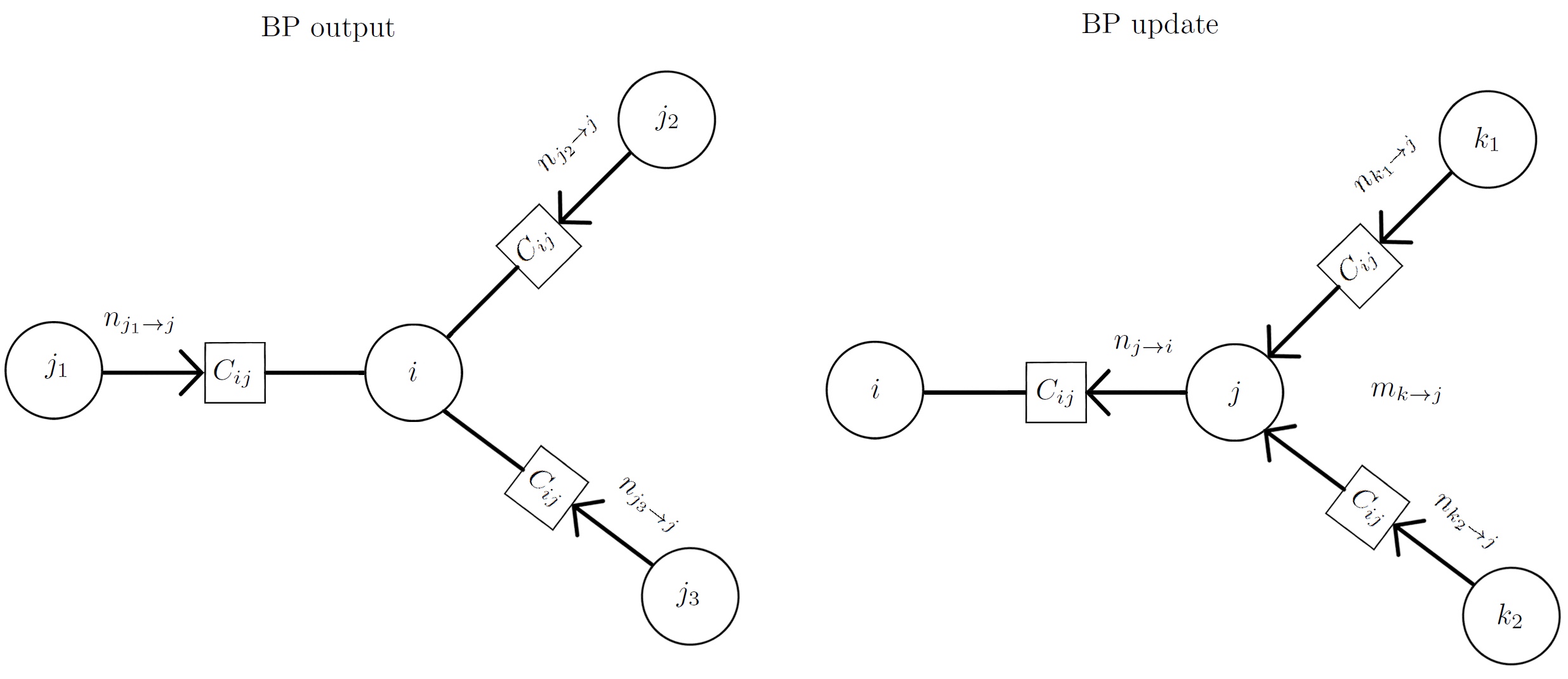
Figure 1: Left panel: illustration of the marginal probability amplitude over local histories as expressed by (2) with cavity assumption (3). Messages $n_{j\to i}$ are equal to $\exp\left(\frac{i}{\hbar}F_{j\rightarrow i}\right)$ where $F_{j\rightarrow i}$ appear in (2), and represent the effect of integrating out nodes in the graph subtended from $j$, but not $j$ itself. Right panel: illustration of the recursive equation satisfied by the messages. Nodes labelled $k$ are here coupled to a node labelled $j$, which in turn is coupled to a node labelled $i$. Message $m_{j\to i}$ is obtained by a double path integral over the histories $X_{j}$ and $Y_{j}$ of node $j$ with the bare action $S_{j}$, the interaction action $S_{ij}$, and the upstream influence $F_{j\rightarrow i}$. This message hence represents integrating out all nodes subtended from node $j$, and node $j$ itself. Message $n_{j\to i}$ is on the hand obtained by combining messages $m_{k\to j}$ for $k$ in the neighborhood of $j$ except $i$. In Section II we discuss harmonic oscillator networks where $n_{j\to i}$ and $m_{j\to i}$ are represented by two pairs of kernels, respectively ($k_{I}^{i\to j},k_{R}^{i\to j},$) and ($\tilde{k}_{I}^{i\to j},\tilde{k}_{R}^{i\to j},$). The BP update equations are then given by (18) and (19) for $m$ to $n$, and, under further assumptions, by (37) and (38) for $n$ to $m$. For further details and the general setting, see Supplementary Information.

Both $m_{j\rightarrow i}$ and $n_{j\rightarrow i}$ are very high-dimensional objects and the update step is therefore in general quite complex and computationally expensive. Further assumptions or approximations are needed to get useful results. A similar problem arises also in classical dynamic cavity Neri and Bollé (2009); Aurell and Mahmoudi (2011, 2012); Del Ferraro and Aurell (2015); Barthel et al. (2018); Barthel (2020); Aurell et al. (2017, 2018, 2019), though there is then only one history per system.

II Uniform harmonic networks

As a solvable example with interesting and indeed unexpected properties, we now a discuss a uniform random network of harmonic oscillators which interact linearly. The action is then $\mathcal{S}[X_{1},\cdots,X_{N}]=\int_{t_{i}}^{t_{f}}\frac{m}{2}\sum_{j}\dot{X}_{j}^{2}-\frac{m\omega^{2}_{0,j}}{2}X^{2}_{j}+\frac{1}{2}\sum_{j,i\in\partial j}C_{ij}(X_{i}-X_{j})^{2}\,dt$ where $m$ is the oscillator mass, $\omega_{0,j}$ is the frequency and $C_{ij}$ is the spring constant between oscillator $i$ and $j$. By a change of scale we can take all oscillators of the same mass. In this section we will also assume all oscillator frequencies the same, and we hence drop the index $j$ on frequency $\omega_{0,j}$. The single-system action parts are $S\left[X_{j}\right]=\int_{t_{i}}^{t_{f}}\frac{m}{2}\dot{X}_{j}^{2}-\frac{m\omega^{2}_{0}+\sum_{i\in\partial j}C_{ij}}{2}X^{2}_{j}\,dt$, and it is convenient to use the notation $m\omega^{2}=m\omega^{2}_{0}+\sum_{i\in\partial j}C_{ij}$. The system-system actions are $S\left[X_{j},X_{k}\right]=\int_{t_{i}}^{t_{f}}\left(-C_{ij}\right)X_{j}X_{k}\,dt$. Eventually we will in this section consider the case when all $C_{ij}$ are the same.

A system of this type can always be solved by diagonalization. However, as except in one dimension the total Hamiltonian is partly random from the structure of the locally tree-like graph, this is not trivial. We will see that the real-time cavity methods offers a more convenient approach, and in fact a way to compute marginals of the diagonalization without actually performing it.

Influence functionals from an environment of harmonic oscillators are parametrized by two kernels, $k_{I}$ which describes dissipation, and $k_{R}$ which describes dispersion Feynman and Vernon (1963). We can therefore introduce a pair of kernels $k_{I}^{i\to j}$ and $k_{R}^{i\to j}$ to parametrize the cavity influence functional $F_{i\to j}$. It is convenient to introduce an analogous cavity functional $\tilde{F}_{i\to j}$ for the $m$-type BP message and its pair of kernels $\tilde{k}_{I}^{i\to j}$ and $\tilde{k}_{R}^{i\to j}$. The two types of kernels are related by

$$k_{I}^{j\rightarrow i}(s,t-s) = \sum_{k\in\partial j\setminus i}\tilde{k}_{I}^{k\rightarrow j}(s,t-s)$$ (4)

$$k_{R}^{j\rightarrow i}(s,t-s) = \sum_{k\in\partial j\setminus i}\tilde{k}_{R}^{k\rightarrow j}(s,t-s)$$ (5)

which is the $m$ to $n$ part of update scheme illustrated in Fig. 1 for harmonic networks.

The 1959 PhD thesis of Frank Vernon Vernon (1959) contains in Appendix V an analysis of the situation where one oscillator ($i$) interacts with another oscillator ($j$), which in turn interacts with a bath of oscillators. The influence of the bath on $j$ is described by an influence action in the forward and backward paths of $j$. Integrating out also $j$ then leads to an influence action in the forward and backward paths of $i$. This Vernon transform was recently discussed by two of us in Aurell and Tuziemski (2021). The same scheme obviously also describes the $n$ to $m$ part of BP update of our concern here. An important special case is when the process has been going on for a long time under constant conditions. In this case the transformation of $k_{I}$ simplify greatly on the Laplace transform side, and reads

$$\tilde{k}_{I}^{j\rightarrow i}(\lambda) = \,\frac{C_{ij}^{2}}{2}G_{0,j}(\lambda)\left(1-G_{0,j}(\lambda){k}_{I}^{j\rightarrow i}(\lambda)\right)^{-1}$$ (6)

where $G_{0,j}(\lambda)=\frac{2}{m}\frac{1}{\lambda^{2}+\omega_{j}^{2}}$ is twice the response function of a free harmonic oscillator with the parameters of oscillator $j$. The imaginary part of the Vernon transform ${\cal V}$ is a nonlinear transformation of ${k}_{I}^{j\rightarrow i}$ to $\tilde{k}_{I}^{j\rightarrow i}$ which acts on each Laplace transform term separately. As it does not depend on the real part, and neither does (18), the imaginary kernels of the cavity influence functionals form a system of updates closed in themselves. This is also true without the assumptions that the process has been going on for a long time under constant conditions. The real part of the Vernon transform ${\cal W}$ is on the other hand a linear transformation of ${k}_{R}^{j\rightarrow i}$ to $\tilde{k}_{R}^{j\rightarrow i}$ which depends quadratically on $\tilde{k}_{I}^{j\rightarrow i}$, i.e. on the image of ${\cal V}$. It simplifies on the Fourier side

$$\tilde{k}_{R}^{j\rightarrow i}(\nu) = \frac{4}{C_{ij}^{2}}|\tilde{k}_{I}^{j\rightarrow i}(\nu)|^{2}k_{R}^{j\rightarrow i}(\nu),$$ (7)

where $\tilde{k}_{I}^{j\rightarrow i}(\nu)$ can be defined directly on the Fourier side, or by analytic continuation from $\tilde{k}_{I}^{j\rightarrow i}(\lambda)$. In any case, the real kernels of the cavity influence functions do not form a system closed in themselves. Furthermore, for a process over a finite time ${\cal W}$ also contain other terms which also depend on $\tilde{k}_{I}^{j\rightarrow i}$ and on initial conditions (bath temperature), but not on $k_{R}^{j\rightarrow i}$, see Supplementary Information.

For a harmonic locally tree-like network we have thus arrived at a system of updates of real numbers where one can look for fixed points. In the uniform network all oscillator frequencies and all interaction parameters are the same ($\omega_{j}=\omega$ for all $j$, $C_{ij}=C$ for pairs $i$ and $j$), and the size of the neighborhood of each system is the same. The includes systems on the line, and systems on random regular graphs. We call the size of the neighborhood of each system $n$ (the line being $n=2$). The uniform fixed point where all kernels everywhere in the network are the same is then on the Laplace transform side given by the fixed point of the one-dimensional map

$$k_{I}^{i+1}(\lambda)=\frac{(n-1)C^{2}}{2}{G}_{0}(\lambda)\left(1-{G}_{0}(\lambda)k_{I}^{i}(\lambda)\right)^{-1}$$ (8)

There is always a fixed point of this rational map for $C$ small enough. When it exists it is given by

$$k_{I}^{*}(\lambda) = m\frac{\lambda^{2}+\omega^{2}}{4}\left(1-\sqrt{1-\frac{8(n-1)\,C^{2}}{m^{2}(\lambda^{2}+\omega^{2})^{2}}}\right)$$ (9)

Given that $\omega^{2}$ has been defined as $\omega^{2}=\omega_{0}^{2}+\frac{nC}{m}$, the expression inside the square root in (70) is a decreasing function of $C$, positive for all $\lambda$ if either $n\geq 8$ or if $n<8$ and $C$ is less than a critical value $C^{*}(n)=\frac{m\omega_{0}^{2}}{\sqrt{8(n-1)}-n}$. For $n<8$ and $C>C^{*}(n)$ the fixed point still exists for $\lambda$ larger than $\lambda^{*}(C,n)=\omega_{0}\sqrt{\frac{C}{C^{*}}-1}$.

The first result on this quite simple example is that if $C<C^{*}$ every system in the uniform network behaves as if interacting with the same effective environment. We call this the ordered phase. The fixed point kernel $k_{I}^{*}$ in the time domain is illustrated in Fig 2; a more detailed discussion can be found in Supplementary Information.

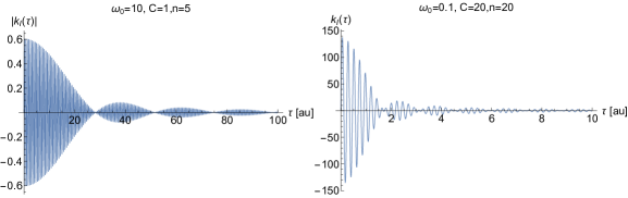
Figure 2: Inverse Laplace transform of the fixed point kernel given by (70). The parameters are: left panel - $\omega_{0}=10$, $C=1$, $n=5$, $m=\frac{1}{2}$; right panel - $\omega_{0}=0.1$, $C=20$, $n=20$, $m=\frac{1}{2}$. One can define an equivalent environment as a set of harmonic oscillators giving rise to the same influence functional acting on oscillator $j$ as the rest of the harmonic network. From the general formula $k_{I}(\tau)=\sum_{b}\frac{1}{2m_{b}\omega_{b}}\sin\omega_{b}\tau$ follows that the spectrum of the equivalent environment, is a band-pass filter with support in the two bands $\pm\sqrt{\omega^{2}\pm\sqrt{8(n-1)}\frac{C}{m}}$. This explains the form of $k_{I}(\tau)$ which has an oscillatory part of frequency $\omega$ and an overlayed breather oscillation. Note that a diagonalization in terms of normal modes must also lead to these kind of formulas, but are not trivial to obtain even for systems on a line.

For $C>C^{*}(n)$ and $\lambda<\lambda^{*}(C,n)$ the BP messages (the functions $k_{I}^{i}(\lambda)$) oscillate as functions of iteration index $i$. In this setting it is therefore not consistent to assume that all incoming messages in Fig. 1 to be the same; there is nothing to synchronize them. As we will discuss in the following Section, one can instead assume that each such $k^{k\rightarrow j}_{I}(\lambda)$ is a random number drawn from a probability $P\left(k^{k\rightarrow j}_{I}(\lambda)\right)$ and check if this distribution is preserved as $P\left(k^{j\rightarrow i}_{I}(\lambda)\right)$ (Replica Symmetric analysis of the BP update equations). In this regime, every system in the uniform network then behaves as if interacting with an environment, drawn from the same distribution of environments. We call this the dynamically disordered phase. The instances of this phase are quite complex, as there is no smooth function $f(t)$ which has a Laplace transform $\tilde{f}(\lambda)$, for which when $\lambda<\lambda^{*}$ the values are independent random numbers. The instances $k_{I}(t-s)$ hence have to be non-smooth mathematical distributions. The seemingly pathological property can be traced back to our neglecting the first time in the definition of $k_{I}(s,t-s)$. In the time domain $k_{I}^{i+1}(s,t-s)$ is related to $k_{I}^{i}(s-\tau_{I},t-s)$ where $\tau_{I}$ is a characteristic time of the response function. When the process starts at time $t_{i}$ one can only iterate the quantum cavity for $i\approx\frac{s-t_{i}}{\tau_{i}}$ times before the initial conditions start to be felt. Therefore, the different components $k_{I}^{i}(s,\lambda)$ are actually correlated over a distance in $\lambda$ of size roughly $\Lambda^{-i}$ where $\Lambda$ is a characteristic expansion rate of the Vernon transform, and $k_{I}^{i}(s,t-s)$ are smooth functions, albeit quite irregular for $s-t_{i}$ much greater than $\tau_{I}$.

When $k_{I}$ is at the fixed point (70), the real Vernon transform (38) is a simple multiplication

$$k_{R}^{i+1}(\nu) = A(\nu)k_{R}^{i}(\nu)$$ (10)

The multiplier $A(\nu)$ depends on whether the square root in (70) (for $\lambda=i\nu$) is positive or negative. The second case pertains to a band of frequencies around $\omega$ with width proportional to $C$. The value is then $2$, while it decreases down from $2$ away from the band. In the ordered phase successive iteration of some Fourier components of $k_{R}$ hence increase without limit. By the same argument as above this pathological behaviour can be traced back to neglecting the first time ; actually $k_{R}(s,\nu)$ only reaches size $2^{\frac{s-t_{i}}{\tau_{i}}}$. Furthermore we have also here neglected additional terms making ${\cal W}$ an affine transformation, see Supplementary Information. In the disordered phase the behaviour of ${\cal W}$ is that of random transform; its analysis will be left to future work.

III Disorder and quantum dynamical Replica Symmetry

Understanding disorder in parameters is an important application of the cavity method. The fixed points of BP will then not be uniform, but the messages $m_{i\rightarrow j}$ and $n_{i\rightarrow j}$ depend on the link in the network. For harmonic networks this means that the Feynman-Vernon fixed point kernels $\left(\tilde{k}_{I}^{i\rightarrow j},\tilde{k}_{R}^{i\rightarrow j}\right)$ and $\left(k_{I}^{i\rightarrow j},k_{R}^{i\rightarrow j}\right)$ are different for different pairs $(i,j)$. We recall how this is analyzed on the level of Replica Symmetry (RS). An ensemble of such networks and interactions are described by probability distributions over the kernel pairs which obey consistency conditions known as RS cavity equations. As the BP update equation acts on $k_{I}$ kernel alone it is convenient to consider separately $P(\tilde{k}_{I})$ and $Q(k_{I})$, which satisfy RS cavity equations

$$Q(k_{I})=\sum_{k}\Lambda_{k}\int\prod_{k}\big{[}d\hat{k}_{I}^{k}P(\hat{k}_{I}^{k})\big{]}\delta(k_{I}-\sum_{k}\hat{k}_{I}^{k})$$ (11)

and

$$P(\hat{k}_{I})=E_{C}\int d\hat{k}_{I}Q(k_{I})\delta(\hat{k}_{I}-{\cal V}(k_{I}))$$ (12)

where $\Lambda_{k}$ is the probability of the neighbourhood to be of size $k$, $E_{c}$ represents the average over the coupling distribution and ${\cal V}$ is the $n$ to $m$ step of the BP update determined by the Vernon transform. The kind of solution discussed above is in this formulation described by $P$’s and $Q$’s that are delta functions.

As we also know from the previous section, even with no disorder in the parameters there is a dynamically disordered phase of the quantum cavity in a uniform network. There is then only one term in the sum in (11), and no average over parameters in (12). Nevertheless, if the Vernon transform does not have a fixed point, the effect is similar. We note that in this setting (11) and (12) can be combined on the Fourier side ($\hat{P}(l)=\int e^{ilx}P(x)dx$) to one update equation

$$\hat{P}^{i+1}(l)=\int dl^{\prime}F(l,l^{\prime})\left(\hat{P}^{i}(l^{\prime})\right)^{n-1}$$ (13)

with the transfer function

$$F(l,l^{\prime})=\frac{1}{2\pi}\int e^{i\left(l^{\prime}{\cal V}(x)+lx\right)}\,dx$$ (14)

For systems on a line ($n=2$) this iteration is simply the Perron-Frobenius transform corresponding to the dynamics given by $x\to{\cal V}(x)$.

IV Discussion and outlook

We have in this work introduced a new real-time version of the quantum cavity method. We have shown that when all systems in a network are harmonic oscillators interacting linearly, this real-time quantum cavity can be represented as transforms of Feynman-Vernon kernels. We have also shown that for uniform harmonic networks where all interaction coefficients in the network are the same, there is an ordered phase where can solve explicitly for a fixed point of transformations. A single quantum harmonic oscillator interacting with a network of quantum harmonic oscillators in the topology of a $n$-regular random graph then behaves as if under the influence of a dissipation kernel of finite spectral support, and eventually arbitrarily strong decoherence, if the dynamics has been going on for a long time. Such a network will hence eventually behave entirely classically.

We have also discussed disorder and Replica Symmetry for real-time quantum cavity. We have pointed out that also the uniform harmonic network has a dynamically disordered phase, in the absence of any disorder in the parameters. Disorder in model parameters induce an Anderson transition on locally tree-like graphs Abou-Chacra et al. (1973); Miller and Derrida (1994); Parisi et al. (2019). For small disorder states are delocalized and influence propagate though the network, while for large disorder states are localized. We conjecture that such a transition also takes place for our real-time problem also. Each system would then perceive the network as an instance of an ensemble of effective environments. To study the properties of these effective environments is an important task for the future.

Finally, the examples we have considered are networks of harmonic oscillators, as they yield explicit solutions of the real-time quantum cavity in closed form. While the challenges in extending these investigations to qubits or other systems are significant there are ways ahead. The first is that the Feynman-Vernon transform is defined for environments that are not harmonic oscillators; the difference being that the Feynman-Vernon action will then have terms cubic, quartic etc in the system variables. The kernels of those higher terms are cumulants of environment correlation functions which vanish for harmonic oscillator baths Aurell et al. (2020). While keeping an an infinite tower of higher-order Feynman-Vernon kernels will surely be impractical, one could consider truncations, such as that the action at every step remains quadratic. Analogous truncations have found many applications in classical information processing Sudderth et al. (2003); Bickson et al. (2009). Another direction is that path integrals for spins have been developed, and it is conceivable that transforms analogous to the Vernon transform could be developed for them also.

Supplementary Information

Contents

1. I The real-time quantum cavity and Replica Symmetry
2. II Uniform harmonic networks
3. III Disorder and quantum dynamical Replica Symmetry
4. IV Discussion and outlook
5. V Details the real-time quantum cavity method for harmonic oscillator networks.
6. VI The Vernon transform in the time domain and on the Laplace transform side
7. VII Representation of the kernel $G$
8. VIII Fixed point for constant interactions on $n$-regular random graphs
   1. VIII.1 First version of the calculation
   2. VIII.2 Second version of the calculation
9. IX Iteration of the real kernel
10. X Stability Analysis of the deterministic Replica Symmetric solution for ferromagnetic model on $n$-regular random graphs

V Details the real-time quantum cavity method for harmonic oscillator networks.

In this section we consider a locally tree-like graph where in each vertex resides a quantum harmonic oscillator. These oscillators interact linearly as indicated by the graph structure.

The starting point of real-time quantum cavity method are the Feynman-Vernon functionals from integrating out a whole tree subtended by one node. As discussed in the main paper these are of two types, conventionally in the cavity literature called ”$n$-type” and and ”$m$-type messages. We introduce parametrizations so that for a harmonic network they read

$$n_{j\rightarrow i}[X_{j},Y_{j}]=e^{\frac{i}{\hbar}F_{j\rightarrow i}[X_{j},Y_{j}]} = \exp\left\{\frac{i}{\hbar}\int^{T}_{\tau}\int^{t}_{\tau}k_{I}^{j\rightarrow i}(s,t-s)\left(X_{j}(t)-Y_{j}(t)\right)\left(X_{j}(s)+Y_{j}(s)\right)dtds\right\}$$ (15)

$$\exp\left\{-\frac{1}{\hbar}\int^{T}_{\tau}\int^{t}_{\tau}k_{R}^{j\rightarrow i}(t,s)\left(X_{j}(t)-Y_{j}(t)\right)\left(X_{j}(s)-Y_{j}(s)\right)\right\}$$

$$m_{j\rightarrow i}[X_{i},Y_{i}]=e^{\frac{i}{\hbar}\tilde{F}_{j\rightarrow i}[X_{i},Y_{i}]} = \exp\left\{\frac{i}{\hbar}\int^{T}_{\tau}\int^{t}_{\tau}\tilde{k}_{I}^{j\rightarrow i}(s,t-s)\left(X_{i}(t)-Y_{i}(t)\right)\left(X_{i}(s)+Y_{i}(s)\right)dtds\right\}$$ (16)

$$\exp\left\{-\frac{1}{\hbar}\int^{T}_{\tau}\int^{t}_{\tau}\tilde{k}_{R}^{j\rightarrow i}(t,s)\left(X_{i}(t)-Y_{i}(t)\right)\left(X_{i}(s)-Y_{i}(s)\right)\right\}$$

The kernels $k^{j\to i}$ (symbol without tilde) in $n_{j\rightarrow i}$ multiply histories pertaining to the ingress node (node $j$). They represent the effect of integrating out the histories of the systems in all nodes neighbours to $j$ or subtended from neighbours of $j$, except node $i$ and nodes subtended from $i$. The kernels $\tilde{k}^{j\to i}$ (symbol with tilde) in $m_{j\rightarrow i}$ multiply histories pertaining to the egress node (node $i$). They represent the effect of integrating out the histories of the systems in node $j$ and nodes subtended from $j$.

One relation between $n$-messages and $m$-messages follow from one of the most basic properties of influence functionals; that influence functions from disjoint environments multiply. In our case we write this as

$$n_{j\rightarrow i}\left[X_{j},Y_{j}\right]\equiv\exp\left[\frac{i}{\hbar}F_{j\rightarrow i}\left[X_{j},Y_{j}\right]\right]=\prod_{k\in\partial j\backslash i}m_{k\rightarrow j}\left[X_{j},Y_{j}\right]\equiv\exp\left[\frac{i}{\hbar}\sum_{k\in\partial j\backslash i}\tilde{F}_{k\rightarrow j}\left[X_{j},Y_{j}\right]\right]$$ (17)

which for the kernels translate to

$$k_{I}^{j\rightarrow i}(s,t-s) = \sum_{k\in\partial j\setminus i}\tilde{k}_{I}^{k\rightarrow j}(s,t-s)$$ (18)

$$k_{R}^{j\rightarrow i}(s,t-s) = \sum_{k\in\partial j\setminus i}\tilde{k}_{R}^{k\rightarrow j}(s,t-s)$$ (19)

The other relation between $n$-messages and $m$-messages follow from integrating out the histories of the system in node $j$ and reads in general

$$m_{k\rightarrow j}\left[X_{j},Y_{j}\right] \equiv \int DX_{k}DY_{k}\exp\left[\frac{i}{\hbar}\left(S\left[X_{k}\right]-S\left[Y_{k}\right]+S\left[X_{j},X_{k}\right]-S\left[Y_{j},Y_{k}\right]\right)\right]$$ (20)

$$\qquad n_{k\rightarrow j}\left[X_{k},Y_{k}\right]\delta(x_{k}(t_{f})-y_{k}(t_{f}))\,\rho_{0}^{(k)}\left(x_{k}(t_{i}),y_{k}(t_{i})\right)$$

For one harmonic oscillator degree of freedom in node $j$ and with interactions as considered here, this is more explicitly

$$e^{\frac{i}{\hbar}\tilde{F}_{j\rightarrow i}[X_{i},Y_{i}]} = \int\exp\left\{\frac{i}{\hbar}\int^{T}_{\tau}\left[\frac{m}{2}\left(\dot{X}_{j}^{2}-\dot{Y}_{j}^{2}\right)-\frac{m\omega^{2}}{2}\left(X^{2}_{j}-Y^{2}_{j}\right)+C_{ij}X_{i}X_{j}-C_{ij}Y_{i}Y_{j}\right]dt\right\}e^{\frac{i}{\hbar}F_{j\rightarrow i}[X_{j},Y_{j}]}$$ (21)

$$\delta\left(X_{j}(T)-Y_{j}(T)\right)\frac{1}{N}\exp\left[-\left(Ax^{2}+2Bxy+Cy^{2}\right)/2\right]{\cal D}X_{j}{\cal D}Y_{j}\,dX_{j}(\tau)dY_{j}(\tau)\,dX_{j}(T)\,dY_{j}(T)$$

Lowercase letters ($x$ and $y$) in above stand for the initial data on $j$, i.e. $X_{j}(\tau)$ and $Y_{j}(\tau)$, and uppercase letters ($X$ and $Y$) will from now on stand for the final data $X_{j}(T)$ and $Y_{j}(T)$. The core problem is to translate (21) into a transformation of kernels. The geometry of passing of message of types $m$ and $n$ is illustrated by Fig. 1

We have required that the initial state in (21) is Gaussian normalized by

$$\hbox{Tr}\left[\rho^{(j)}(\tau)\right]=\frac{1}{N}\int dx\exp\left[-\left(A+2B+C\right)x^{2}/2\right]=1$$ (22)

and we will later require that it is symmetric, $A=C$. Eq. (21) is then precisely the kind of iterated path integral studied by Vernon in Appendix V of his PhD thesis Vernon (1959) and which we call the Vernon transform. We can therefore immediately write down

$$\tilde{k}_{I}^{j\rightarrow i} = \,{\cal V}\left[k_{I}^{j\to i},C_{ij}\right]$$ (23)

$$= C_{ij}(t)\,C_{ij}(s)\,G^{j\to i}(t,s-t)$$

where the response function and the friction kernel satisfies the twinning relation

$$G^{j\to i}(t,s-t) = G_{j}^{(0)}(s-t)+\int_{t}^{T}dt_{1}\int_{t_{1}}^{T}dt_{2}\,G_{j}^{(0)}(t_{1}-t)$$ (24)

$$\quad k_{I}^{k\rightarrow j}(t_{1},t_{2}-t_{1})\,G^{j\to i}(t_{2},s-t_{2})$$

In above $G_{j}^{(0)}(s-t)$ is twice the response function of oscillator $j$ without the friction kernel given by $k_{I}^{j\to i}$. For derivations, see Sections VI and VII.

The real side of the Vernon transform ${\cal W}$ is in general the sum of three terms. All three depend quadratically on the response function $G^{j\to i}$, one depends linearly on $k_{R}^{j\rightarrow i}$ and two terms do not depend on $k_{R}^{j\rightarrow i}$.

With $A^{\prime}=\frac{1}{2}\left(A+B\right)$ and $C^{\prime}=\frac{1}{2}\left(A-B\right)$ characterizing the initial symmetric state of oscillator $j$ the three terms read

$$\tilde{k}_{R}^{j\rightarrow i}(t,s) = C_{ij}(t)\,C_{ij}(s)\,\int_{\tau}^{t}\int_{\tau}^{s}k_{R}^{j\rightarrow i}(t^{\prime},s^{\prime})\,G^{j\to i}(t^{\prime},t-t^{\prime})\,G^{j\to i}(s^{\prime},s-s^{\prime})\,ds^{\prime}dt^{\prime}\,+\,$$ (25)

$$C_{ij}(t)\,C_{ij}(s)\,\left(\hbar C^{\prime}G^{j\to i}(\tau,t-\tau)\,G^{j\to i}(\tau,s-\tau)+\,\frac{1}{\hbar A^{\prime}}\frac{dG^{j\to i}(r,t-r)}{dr}|_{r=\tau}\,\,\frac{dG^{j\to i}(r,s-r)}{dr}|_{r=\tau}\right)$$

The last two terms in (25) stem from the initial condition of oscillator $j$. They are in fact the same terms that give rise to the quantum noise kernel $k_{R}$ in Vernon’s original derivation of the Feynman-Vernon kernels (Vernon (1959), Appendix I). Under conditions discussed in Section VI these two terms vanish in several settings when the process goes on for an infinite time ($\tau=-\infty$). Also, when $G^{j\to i}$ behaves as the response function of a damped harmonic oscillator it has finite memory, and the two last terms in (25) are boundary contributions which only matter in the beginning of the process (both times $t$ and $s$ close to $\tau$).

Furthermore, the Vernon transforms ${\cal V}$ and ${\cal W}$ simplify considerably on the Laplace/Fourier side when the interaction coefficients $C_{\alpha}$ (all pairs $\alpha$) do not depend on time, all real kernels $k_{R}(\cdot,t)$ only depend on the second time argument, and all imaginary kernels $k_{R}(t,s)$ only depend on the time difference.

The twinning equation can thus be written on the Laplace transform side as

$$\tilde{G}^{j\to i}(\lambda) = \tilde{G}_{j}^{(0)}(\lambda)\left(1+\tilde{k}_{I}^{k\rightarrow j}(\lambda)\,\tilde{G}^{j\to i}(\lambda)\right)$$ (26)

The above form was used for the fixed point calculations in the main body of the paper.

VI The Vernon transform in the time domain and on the Laplace transform side

This Section contains further details on the calculation outlined in the previous section. It starts with a presentation of the Vernon transform (Vernon (1959), Appendix V); this material can also be found in Aurell and Tuziemski (2021). In contrast to that earlier presentation we keep the time dependence throughout, to eventually write the Vernon transform for a time-stationary situation on the Laplace side.

The point of departure is (21), the path integral expressing the Vernon transform. For illustration, for the moment we do not require the initial state to be symmetric. One introduces the new variables

$$\bar{X}_{j}(t)=X_{j}(t)+Y_{j}(t)$$ (27)

$$\Delta_{j}(t)=X_{j}(t)-Y_{j}(t)$$ (28)

and similarly for the target node $i$ and the initial and final state on $j$. In this way one can write

$$e^{\frac{i}{\hbar}\tilde{F}_{j\rightarrow i}[\bar{X}_{i},\Delta_{i}]}= \int\delta\left(\Delta_{j}^{T}\right)\exp\left\{\frac{i}{\hbar}\int^{T}_{\tau}\left[\left(\frac{m}{2}\dot{\bar{X}}_{j}\dot{\Delta}_{j}-\frac{m\omega^{2}}{2}\bar{X}_{j}\Delta_{j}+\frac{C_{ij}}{2}\bar{X}_{i}\Delta_{j}+\frac{C_{ij}}{2}\Delta_{i}\bar{X}_{j}\right)\right]dt\right\}$$ (29)

$$\qquad\exp\left\{\frac{i}{\hbar}\int^{T}_{\tau}\int^{t}_{\tau}k_{I}^{j\rightarrow i}(s,t-s)\Delta_{j}(t)\bar{X}_{j}(s)dtds-\frac{1}{\hbar}\int^{T}_{\tau}\int^{t}_{\tau}k_{R}^{j\rightarrow i}(t,s)\Delta_{j}(t)\Delta_{j}(s)dtds\right\}$$

$$\frac{1}{N}\exp\left[-\left(A^{\prime}(\bar{X}_{j}^{\tau})^{2}+2B^{\prime}\bar{X}_{j}^{\tau}\Delta_{j}^{\tau}+C^{\prime}(\Delta_{j}^{\tau})^{2}\right)/2\right]\,{\cal D}\bar{X}_{j}{\cal D}\Delta_{j}\,d\Delta_{j}^{\tau}d\Delta_{j}^{T}d\bar{X}_{j}^{\tau}d\bar{X}_{j}^{T}$$

where $A^{\prime}=\frac{1}{4}\left(A+2B+C\right)$ $C^{\prime}=\frac{1}{4}\left(A-2B+C\right)$, and $B^{\prime}=\frac{1}{2}\left(A-C\right)$. Requiring that the initial state does not mix $\bar{x}_{j}$ and $\Delta_{j}$ leads to $B^{\prime}=0$ and the expressions used in (25) above. Those are $A^{\prime}=\frac{1}{2}\left(A+B\right)$ and $C^{\prime}=\frac{1}{2}\left(A-B\right)$. Note that the normalization $\frac{1}{N}\int e^{-\frac{1}{2}(A^{\prime}\bar{x}^{2})}d\bar{x}=2$. A thermal state at inverse temperature $\beta$ has $A=C=\frac{m_{j}\omega_{j}}{\hbar}\coth{\beta\hbar\omega_{j}}$ and $B=-\frac{m_{j}\omega_{j}}{\hbar}\sinh^{-1}{\beta\hbar\omega_{j}}$, and hence $A^{\prime}=\frac{m_{j}\omega_{j}}{2\hbar}\tanh{\frac{\beta\hbar\omega_{j}}{2}}$ and $C^{\prime}=\frac{m_{j}\omega_{j}}{2\hbar}\coth{\frac{\beta\hbar\omega_{j}}{2}}$. The assumption of an initially symmetric Gaussian state is hence equivalent to assuming an initial thermal state where the two parameters $A^{\prime}$ and $C^{\prime}$ set a length scale $\ell=\frac{2\hbar}{m_{j}\omega_{j}}=\frac{1}{\sqrt{A^{\prime}C^{\prime}}}$ and an inverse temperature $\beta=\frac{2}{\hbar\omega_{j}}\tanh^{-1}{\sqrt{\frac{A^{\prime}}{C^{\prime}}}}$. We will drop the primes on $A^{\prime}$ and $C^{\prime}$ from now on.

The first step is now to integrate the term $\dot{\bar{X}}_{j}\dot{\Delta}_{j}$ by parts which gives

$$\int_{\tau}^{T}\dot{\bar{X}}_{j}\dot{\Delta}_{j}dt = \dot{\Delta}_{j}^{T}\bar{X}_{j}^{T}-\dot{\Delta}_{j}^{\tau}\bar{X}_{j}^{\tau}-\int_{\tau}^{T}\bar{X}_{j}\ddot{\Delta}_{j}dt$$ (30)

from which follows

$$e^{\frac{i}{\hbar}\tilde{F}_{j\rightarrow i}[\bar{X}_{i},\Delta_{i}]}= \frac{1}{2}\int\delta\left(\Delta_{j}^{T}\right)\exp\left\{\frac{i}{\hbar}\int^{T}_{\tau}\left[\left(-\frac{m}{2}\bar{X}_{j}\ddot{\Delta}_{j}-\frac{m\omega^{2}}{2}\bar{X}_{j}\Delta_{j}+\frac{C_{ij}}{2}\bar{X}_{i}\Delta_{j}+\frac{C_{ij}}{2}\Delta_{i}\bar{X}_{j}\right)\right]dt\right\}$$ (31)

$$\qquad\exp\left\{\frac{i}{\hbar}\int^{T}_{\tau}\int^{t}_{\tau}k_{I}^{j\rightarrow i}(s,t-s)\Delta_{j}(t)\bar{X}_{j}(s)dtds-\frac{1}{\hbar}\int^{T}_{\tau}\int^{t}_{\tau}k_{R}^{j\rightarrow i}(t,s)\Delta_{j}(t)\Delta_{j}(s)dtds\right\}$$

$$\frac{1}{N}\exp\left[-\left(A^{\prime}\bar{X_{j}^{\tau}}^{2}+C^{\prime}(\Delta_{j}^{\tau})^{2}\right)/2\right]\,\exp\frac{im}{2\hbar}(\dot{\Delta}_{j}^{T}\bar{X}_{j}^{T}-\dot{\Delta}_{j}^{\tau}\bar{X}_{j}^{\tau}){\cal D}\bar{X}_{j}{\cal D}\Delta_{j}\,d\Delta_{j}^{\tau}d\Delta_{j}^{T}d\bar{X}_{j}^{\tau}d\bar{X}_{j}^{T}$$

The pre-factor $\frac{1}{2}$ is the Jacobian of the change of variables at the initial time; the other (functional) Jacobian is included in the path integral measure. The initial state is Gaussian and we can integrate over $\bar{X}_{j}$. This gives $\frac{1}{N}\int d\bar{X}_{j}^{\tau}e^{-\frac{1}{2}A^{\prime}\bar{X_{j}^{\tau}}^{2}-\frac{im}{2\hbar}\dot{\Delta}_{j}^{\tau}\bar{X}_{j}^{\tau}}=2e^{-\frac{m^{2}}{8\hbar^{2}A^{\prime}}(\dot{\Delta}_{j}^{\tau})^{2}}$ where the factor $2$ cancels in above. The corresponding integral over the final state fixes the final velocity for $\Delta_{j}$, that is $\int d\bar{X}_{j}^{T}\exp^{\frac{im}{2\hbar}\dot{\Delta}_{j}^{T}\bar{X}_{j}^{T}}=\delta(\dot{\Delta}_{j}^{T})$. The remaining integrals over $\bar{X}_{j}$ at intermediate times give a delta-functional

$$\delta(g(\Delta_{j})(t))$$ (32)

where

$$g(\Delta_{j})(t) = \frac{m}{2}\ddot{\Delta}_{j}(t)+\frac{m\omega^{2}}{2}\Delta_{j}(t)-\frac{C_{ij}}{2}\Delta_{i}(t)-\int^{T}_{t}k_{I}^{j\rightarrow i}(t,s-t)\Delta_{j}(s)ds.$$ (33)

The integral over the deviation path $\Delta_{j}(t)$ hence has support on a classical path which satisfies final conditions $\Delta_{j}=\dot{\Delta}_{j}=0$, and equations of motion $g(\Delta X_{j})(t)=0$. It is convenient to call this auxiliary path $Q(t)$. The double path integral in (31) hence gives

$$\frac{i}{\hbar}\tilde{F}_{j\rightarrow i}[\bar{X}_{i},\Delta X_{i}] = \frac{i}{\hbar}\int_{\tau}^{T}\frac{C_{ij}(t)}{2}\bar{X}_{i}(t)Q(t)dt-\frac{1}{2\hbar}\int_{\tau}^{T}\int_{\tau}^{T}k_{R}^{j\rightarrow i}(t,s)Q(t)Q(s)-\frac{1}{2}Cq^{2}-\frac{m^{2}}{8\hbar^{2}A}(\dot{q})^{2}$$ (34)

where by $q$ we mean the initial position of the auxiliary classical path, i.e. $Q(\tau)$. $Q(t)$ depends on the deviation path $\Delta X_{i}(s)$ for all values of $s$ larger than $t$. This is because $Q$ satisfies final conditions as $s=T$ while its initial conditions at $s=\tau$ are not given. It is further clear that $Q(t)$ is a linear functional $\Delta X_{i}(s)$ for $s\in\left[t,T\right]$. This linear functional can be represented by a kernel

$$Q(t)=\int_{t}^{T}G(t,s-t)\,C_{ij}(s)\Delta X_{j}(s)\,ds$$ (35)

where

$$G(t,s-t)=G_{0}(s-t)+\int_{t}^{T}dt_{1}\int_{t_{1}}^{\infty}dt_{2}G_{0}(t_{1}-t)k_{I}^{k\rightarrow j}(t_{1},t_{2}-t_{1})G(t_{2},s-t_{2})$$ (36)

As shown in Section VII there is at least as a formal power series there is a kernel which satisfies $G(t,s-t)=0$ for $s<t$. Substituting (35) in (34) we have the kernels of the transformed Feynman-Vernon action as

$$\tilde{k}_{I}^{j\rightarrow i}(t,s-t) = \frac{1}{2}\,C_{ij}(t)\,C_{ij}(s)\,G(t,s-t)$$ (37)

$$\tilde{k}_{R}^{j\rightarrow i}(t,s) = C_{ij}(t)\,C_{ij}(s)\,\int_{\tau}^{t}\int_{\tau}^{s}k_{R}^{j\rightarrow i}(t^{\prime},s^{\prime})\,G(t^{\prime},t-t^{\prime})\,G(s^{\prime},s-s^{\prime})\,ds^{\prime}dt^{\prime}$$ (38)

$$\quad+\,C_{ij}(t)\,C_{ij}(s)\,\hbar CG(\tau,t+\tau)\,G(\tau,s+\tau)$$

$$\qquad+\,C_{ij}(t)\,C_{ij}(s)\,\frac{1}{\hbar A}\frac{dG(r,t-r)}{dr}|_{r=\tau}\,\,\frac{dG(r,s-r)}{dr}|_{r=\tau}\,\,$$

The last two terms are zero if the auxiliary path $Q(t)$ returns to rest at the origin at $t\to\tau$. This should be so whenever the kernel $k_{I}^{j\rightarrow i}(t,s-t)$ behaves as friction and when the process goes on for infinite time ($\tau=-\infty$), and when the drive ($C_{ij}(t)$) vanishes before some turn-on time $t_{i}$. In any case, if the response function $G(\tau,t+\tau)$ has essentially finite support in $t$, these two terms will only give a boundary contribution, and will not matter when $t$ and $s$ are sufficiently larger than $\tau$.

In this way we have formally established the BP update equation as an integral transformation on Feynman-Vernon kernels given by (37) and the first line of (38). Equations, (37) and (38), can be closed through the use of (17). Concretely we write them as

$$k_{I}^{j\rightarrow i}(t,s-t) = \sum_{k\in\partial j/i}\tilde{k}_{I}^{k\rightarrow j}(t,s-t)=\sum_{k\in\partial j/i}\frac{1}{2}\,C_{kj}(t)\,C_{kj}(s)\,G(t,s-t)$$

$$k_{R}^{j\rightarrow i}(t,s) = \sum_{k\in\partial j/i}\tilde{k}_{R}^{k\rightarrow j}(t,s)=\sum_{k\in\partial j/i}C_{kj}(t)\,C_{kj}(s)\,\int_{-\infty}^{t}\int_{-\infty}^{s}k_{R}^{k\rightarrow j}(t^{\prime},s^{\prime})\,G(t^{\prime},t-t^{\prime})\,G(s^{\prime},s-s^{\prime})\,ds^{\prime}dt^{\prime}$$ (39)

Note that the information about the graph structure is given through the introduction of the $\sum_{k\in\partial j/i}$.

VII Representation of the kernel $G$

The goal of this Section is to derive an explicit representation of the kernel $G$ defined in (35) in the preceding Section. This kernel is to relate a function $Q(t)$ to a source term $C_{ij}(s)\Delta X_{i}(s)$ for all $s>t$. Values of the source at times $s$ earlier than $t$ have no influence on $Q(t)$. The solution must therefore satisfy $G(t,s-t)=0$ when $s<t$.

$Q(t)$ is determined by the equation of motion of an externally driven harmonic oscillator with non-Markovian damping (given in preceding appendix as (33) (and below as (40)) and final conditions $Q(T)=\dot{Q}(T)=0$. For an infinite time interval ($\tau=-\infty$ and $T=\infty$) it is convenient to assume that $C_{ij}(s)$ vanishes for $s>t_{f}$ as well as for $s<t_{i}$. The first means that $Q(t)$ must also vanish for $t>t_{f}$. The second means that for those values $Q$ satisfies an autonomous integro-differential equation without drive. That is, if we know $Q$ in the interval $[t_{i}:t_{f}]$ then $Q(t)$ for $t<t_{i}$ follows as a consequence.

For convenience we restate the equation satisfied by $Q$ representing oscillator $k$ driven by oscillator $j$:

$$\frac{m}{2}\ddot{Q}+\frac{m\omega^{2}}{2}Q-\frac{1}{2}C_{kj}(t)\Delta_{j}(t)-\int_{t}^{\infty}dsk_{I}^{k\rightarrow j}(t,s-t)Q(s)=0$$ (40)

To emphasize that $k_{I}^{k\rightarrow j}(t,s-t)$ we write out explicitly a Heaviside function $\Theta(s-t)$. We start introducing the Fourier transform of

$$Q(t)=\frac{1}{2\pi}\int_{-\infty}^{\infty}d\nu e^{-i\nu t}\hat{Q}(\nu)$$ (41)

and

$$k_{I}^{k\rightarrow j}(t,s-t)\Theta[s-t]=\frac{1}{2\pi}\int_{-\infty}^{\infty}d\mu e^{-i\mu(s-t)}\hat{k}_{I^{-}}^{k\rightarrow j}(t,\mu)$$ (42)

where $\mu$ should have an infinitesimal positive imaginary part. Substituted in Eq. (40) this leads to

$$\frac{1}{2\pi}\int d\nu e^{-i\nu t}\Bigg{[}\frac{m}{2}(-\nu^{2}+\omega^{2})\hat{\Delta}_{k}(\nu)-\frac{1}{2}\Big{[}C_{kj}\Delta_{j}\Big{]}_{\nu}-\hat{k}_{I^{-}}^{k\rightarrow j}(t,-\nu)\hat{\Delta}_{k}(\nu)\Bigg{]}=0$$ (43)

where $\nu$ should have an infinitesimal negative imaginary part.

Integrating over time, $\int dte^{i\kappa t}$

$$\frac{1}{2\pi}\int dte^{i\kappa t}\int d\nu e^{-i\nu t}\Bigg{[}\frac{m}{2}(-\nu^{2}+\omega^{2})\hat{\Delta}_{k}(\nu)-\frac{1}{2}\Big{[}C_{kj}\Delta_{j}\Big{]}_{\nu}-\hat{k}_{I^{-}}^{k\rightarrow j}(t,-\nu)\hat{\Delta}_{k}(\nu)\Bigg{]}=0$$ (44)

and defining

$$\hat{\hat{k}}_{I^{-}}^{k\rightarrow j}(\kappa-\nu,-\nu)=\int_{-\infty}^{\infty}dte^{i(\kappa-\nu)t}\hat{k}_{I^{-}}^{k\rightarrow j}(t,-\nu)$$ (45)

one finds:

$$\Bigg{[}\frac{m}{2}(-\kappa^{2}+\omega^{2})\hat{Q}(\kappa)-\frac{1}{2}\Big{[}C_{kj}\Delta_{j}\Big{]}_{\kappa}-\frac{1}{2\pi}\int_{-\infty}^{\infty}d\nu\hat{\hat{k}}_{I^{-}}^{k\rightarrow j}(\kappa-\nu,-\nu)\hat{Q}(\nu)\Bigg{]}=0$$ (46)

where $\kappa$ should have an infinitesimal negative imaginary part.

We can re-write the preceding expression as

$$\hat{Q}(\kappa)=\frac{\frac{1}{2}\Big{[}C_{kj}\Delta_{j}\Big{]}_{\kappa}}{\frac{m}{2}(\omega^{2}-\kappa^{2})}+\frac{\frac{1}{2\pi}\int_{-\infty}^{\infty}d\nu\hat{\hat{k}}_{I^{-}}^{k\rightarrow j}(\kappa-\nu,-\nu)\hat{Q}(\nu)}{\frac{m}{2}(\omega^{2}-\kappa^{2})}$$ (47)

which is a Fredholm singular integral. This can be written as

$$\hat{Q}(\kappa)=f(\kappa)+\lambda\int_{-\infty}^{\infty}d\nu K(\kappa,\nu)\hat{Q}(\nu)$$ (48)

Applying the method of successive iterated approximations one finds

$$\hat{Q}(\kappa) = f(\kappa)+\lambda\int_{-\infty}^{\infty}d\nu K(\kappa,\nu)f(\nu)+$$

$$+ \lambda^{2}\int_{-\infty}^{\infty}\int_{-\infty}^{\infty}d\nu d\nu_{1}K(\kappa,\nu)K(\nu,\nu_{1})f(\nu_{1})+$$

$$+ \lambda^{2}\int_{-\infty}^{\infty}\int_{-\infty}^{\infty}\int_{-\infty}^{\infty}d\nu d\nu_{1}d\nu_{2}K(\kappa,\nu)K(\nu,\nu_{1})K(\nu_{1},\nu_{2})f(\nu_{2})+$$

$$\cdots$$

Substituting for our $f(\kappa)$ and $K(\kappa,\nu)$ one finds

$$\hat{Q}(\kappa) = \frac{\frac{1}{2}\Big{[}C_{kj}\Delta_{j}\Big{]}_{\kappa}}{\frac{m}{2}(\omega^{2}-\kappa^{2})}+\int_{-\infty}^{\infty}d\nu\frac{\frac{1}{2\pi}\hat{\hat{k}}_{I^{-}}^{k\rightarrow j}(\kappa-\nu,-\nu)}{\frac{m}{2}(\omega^{2}-\kappa^{2})}\frac{\frac{1}{2}\Big{[}C_{kj}\Delta_{j}\Big{]}_{\nu}}{\frac{m}{2}(\omega^{2}-\nu^{2})}+$$

$$+ \int_{-\infty}^{\infty}\int_{-\infty}^{\infty}d\nu d\nu_{1}\frac{\frac{1}{2\pi}\hat{\hat{k}}_{I^{-}}^{k\rightarrow j}(\kappa-\nu,-\nu)}{\frac{m}{2}(\omega^{2}-\kappa^{2})}\frac{\frac{1}{2\pi}\hat{\hat{k}}_{I^{-}}^{k\rightarrow j}(\nu-\nu_{1},-\nu_{1})}{\frac{m}{2}(\omega^{2}-\nu^{2})}\frac{\frac{1}{2}\Big{[}C_{kj}\Delta_{j}\Big{]}_{\nu_{1}}}{\frac{m}{2}(\omega^{2}-\nu_{1}^{2})}$$

$$+ \int_{-\infty}^{\infty}\int_{-\infty}^{\infty}\int_{-\infty}^{\infty}d\nu d\nu_{1}d\nu_{2}\frac{\frac{1}{2\pi}\hat{\hat{k}}_{I^{-}}^{k\rightarrow j}(\kappa-\nu,-\nu)}{\frac{m}{2}(\omega^{2}-\kappa^{2})}\frac{\frac{1}{2\pi}\hat{\hat{k}}_{I^{-}}^{k\rightarrow j}(\nu-\nu_{1},-\nu_{1})}{\frac{m}{2}(\omega^{2}-\nu^{2})}\frac{\frac{1}{2\pi}\hat{\hat{k}}_{I^{-}}^{k\rightarrow j}(\nu_{1}-\nu_{2},-\nu_{2})}{\frac{m}{2}(\omega^{2}-\nu_{1}^{2})}\frac{\frac{1}{2}\Big{[}C_{kj}\Delta_{j}\Big{]}_{\nu_{2}}}{\frac{m}{2}(\omega^{2}-\nu_{2}^{2})}+$$

$$+\cdots$$

The above expression can be written as $Q(t)=\int_{-\infty}^{\infty}ds\frac{1}{2}G(t,s)C_{kj}(s)\Delta_{j}(s)$ where $G(t,s)$ stands for the iterated sum

$$G(t,s) = \Bigg{[}\frac{1}{2\pi}\int_{-\infty}^{\infty}d\kappa e^{-i\kappa t}\frac{1}{\frac{m}{2}(\omega^{2}-\kappa^{2})}e^{i\kappa s}+$$

$$+ \frac{1}{2\pi}\int_{-\infty}^{\infty}d\kappa e^{-i\kappa t}\frac{1}{\frac{m}{2}(\omega^{2}-\kappa^{2})}\int_{-\infty}^{\infty}d\nu\frac{\frac{1}{2\pi}\hat{\hat{k}}_{I^{-}}^{k\rightarrow j}(\kappa-\nu,-\nu)}{\frac{m}{2}(\omega^{2}-\nu^{2})}e^{i\nu s}+$$

$$+ \frac{1}{2\pi}\int_{-\infty}^{\infty}d\kappa e^{-i\kappa t}\frac{1}{\frac{m}{2}(\omega^{2}-\kappa^{2})}\int_{-\infty}^{\infty}\int_{-\infty}^{\infty}d\nu d\nu_{1}\frac{\frac{1}{2\pi}\hat{\hat{k}}_{I^{-}}^{k\rightarrow j}(\kappa-\nu,-\nu)}{\frac{m}{2}(\omega^{2}-\nu^{2})}\frac{\frac{1}{2\pi}\hat{\hat{k}}_{I^{-}}^{k\rightarrow j}(\nu-\nu_{1},-\nu_{1})}{\frac{m}{2}(\omega^{2}-\nu_{1}^{2})}e^{i\nu_{1}s}+\cdots\Bigg{]}$$

The first (zero order) term in the sum

$$G_{0}(t,s)=\frac{1}{2\pi}\int_{-\infty}^{\infty}d\kappa e^{i\kappa(s-t)}\frac{1}{\frac{m}{2}(\omega^{2}-\kappa^{2})}$$ (52)

When $\kappa$ has infinitesimal negative imaginary part and when $s-t$ is negative, the integral can be closed in the lower half plane, and is zero. When $s-t$ is positive the integral can be closed in the upper complex plane and is $\frac{2}{m\omega}\sin\omega(s-t)$.

The next (first order) term is

$$G_{1}(t,s) = \frac{1}{2\pi}\int_{-\infty}^{\infty}d\kappa e^{-i\kappa t}\frac{1}{\frac{m}{2}(\omega^{2}-\kappa^{2})}\int_{-\infty}^{\infty}d\nu\frac{e^{i\nu s}}{\frac{m}{2}(\omega^{2}-\nu^{2})}\frac{1}{2\pi}\hat{\hat{k}}_{I^{-}}^{k\rightarrow j}(\kappa-\nu,-\nu)=$$

$$= \frac{1}{2\pi}\int_{-\infty}^{\infty}d\kappa\frac{e^{-i\kappa t}}{\frac{m}{2}(\omega^{2}-\kappa^{2})}\int_{-\infty}^{\infty}d\nu\frac{e^{i\nu s}}{\frac{m}{2}(\omega^{2}-\nu^{2})}\frac{1}{2\pi}\int_{-\infty}^{\infty}dt_{1}e^{i(\kappa-\nu)t_{1}}\hat{k}_{I^{-}}^{k\rightarrow j}(t_{1},-\nu)=$$

$$= \frac{1}{2\pi}\int_{-\infty}^{\infty}d\kappa\frac{e^{-i\kappa t}}{\frac{m}{2}(\omega^{2}-\kappa^{2})}\int_{-\infty}^{\infty}d\nu\frac{e^{i\nu s}}{\frac{m}{2}(\omega^{2}-\nu^{2})}\frac{1}{2\pi}\int_{-\infty}^{\infty}dt_{1}e^{i(\kappa-\nu)t_{1}}\int_{-\infty}^{\infty}dt_{2}e^{-i\nu(t_{2}-t_{1})}k_{I}^{k\rightarrow j}(t_{1},t_{2}-t_{1})\Theta(t_{2}-t_{1})$$

where the definitions of $\hat{\hat{k}}_{I^{-}}^{k\rightarrow j}(\kappa-\nu,-\nu)$ and $\hat{k}_{I}^{k\rightarrow j}(t,-\nu)$ given in Eqs. (45) and (45) were used. In the above some term can be rearranged to give

$$G_{1}(t,s) = \frac{1}{2\pi}\int_{-\infty}^{\infty}dt_{1}\int_{-\infty}^{\infty}dt_{2}\frac{1}{2\pi}k_{I}^{k\rightarrow j}(t_{1},t_{2}-t_{1})\Theta(t_{2}-t_{1})\int_{-\infty}^{\infty}d\kappa\frac{e^{-i\kappa(t-t_{1})}}{\frac{m}{2}(\omega^{2}-\kappa^{2})}\int_{-\infty}^{\infty}d\nu\frac{e^{i\nu(s-t_{2})}}{\frac{m}{2}(\omega^{2}-\nu^{2})}=$$

$$= \int_{-\infty}^{\infty}dt_{1}\int_{t_{1}}^{\infty}dt_{2}k_{I}^{k\rightarrow j}(t_{1},t_{2}-t_{1})\frac{1}{2\pi}\int_{-\infty}^{\infty}d\kappa\frac{e^{-i\kappa(t-t_{1})}}{\frac{m}{2}(\omega^{2}-\kappa^{2})}\frac{1}{2\pi}\int_{-\infty}^{\infty}d\nu\frac{e^{i\nu(s-t_{2})}}{\frac{m}{2}(\omega^{2}-\nu^{2})}=$$

$$= \int_{-\infty}^{\infty}dt_{1}\int_{t_{1}}^{\infty}dt_{2}k_{I}^{k\rightarrow j}(t_{1},t_{2}-t_{1})G_{0}(t_{1}-t)G_{0}(s-t_{2})$$

Successive repetition of the above procedure leads to the following expression

$$G(t,s-t)=G_{0}(s-t)+\int_{t}^{T}dt_{1}\int_{t_{1}}^{T}dt_{2}G_{0}(t_{1}-t)k_{I}^{k\rightarrow j}(t_{1},t_{2}-t_{1})G(t_{2},s-t_{2}),$$ (55)

which is Eq (24). In general, the above one-sided functional equation does not have a convenient closed-form solution. However, if one assumes that both $k_{I}^{k\rightarrow j}(t,s-t)$ and $G(t,s-t)$ depend only on their second argument and essentially vanish when it is large enough, one has the considerably simpler relation

$$G(s-t)=G_{0}(s-t)+\int_{t}^{\infty}dt_{1}\int_{t_{1}}^{\infty}dt_{2}G_{0}(t_{1}-t)k_{I}^{k\rightarrow j}(t_{2}-t_{1})G(s-t_{2})$$ (56)

valid when $s$ (the largest time in above) is considerably smaller than $T$ (the final time). Since this equation involves a convolution, it can be conveniently written in the Laplace domain as

$$\tilde{G}(\lambda)=\tilde{G}_{0}(\lambda)+\tilde{G}_{0}(\lambda)k_{I}^{k\rightarrow j}(\lambda)\tilde{G}(\lambda),$$ (57)

where for simplicity we used the same symbol for $k_{I}^{k\rightarrow j}$ in the time domain and in the Laplace domain. The Laplace transform $\tilde{G}_{0}(\lambda)$ is given by

$$\tilde{G}_{0}(\lambda) = \int_{0}^{\infty}e^{-\lambda t}\frac{2}{m\omega}\sin\omega t\,dt=\frac{2}{m}\frac{1}{\lambda^{2}+\omega^{2}}$$ (58)

This is twice the response function of the harmonic oscillator as conventionally defined.

VIII Fixed point for constant interactions on $n$-regular random graphs

The goal of this section is to make an explicit computation of (39) in a specific model. We will present two approaches, one relying on the known representation of the Laplace transform function, and one of a sine transform analogous to the the Mehler–Sonine representation of the Bessel function. We consider a set of oscillators interacting with constant couplings, what one may call a ferromagnetic case. In the present context constant interaction means that all functions $C_{ij}(t)$ are the same and do not depend on time. Moreover, we will assume that oscillators are placed in an $n$-regular random graphs, i.e. a graph where all vertices have the same number ($n$) of neighbours. In such a setting there can be a deterministic Replica Symmetric phase of the cavity equations where all cavity messages are the same. In this section we will consider the corresponding fixed point and the corresponding message.

In this case, it is easy to show that:

$$\tilde{k}_{I}^{k\rightarrow j}(t,s-t) =\frac{1}{2}C_{kj}C_{kj}G^{k\rightarrow j}(t,s-t)$$ (59)

$$\tilde{k}_{R}^{k\rightarrow j}(t,s) =C_{kj}C_{kj}\int_{-\infty}^{t}\int_{-\infty}^{s}k_{R}^{k\rightarrow j}(t^{\prime},s^{\prime})G^{k\rightarrow j}(t^{\prime},t-t^{\prime})G^{k\rightarrow j}(s^{\prime},s-s^{\prime})$$ (60)

These expression apparently suggest that the sign of the couplings $C_{ij}$ is irrelevant, they always appear squared. However, we have to remember that in above we have implicitly used the relation $\omega^{2}=\omega_{0}^{2}+\frac{nC}{m}$ which enters in the bare response function $G_{0}$, which in turn enters in $G$. $C$ can be taken arbitrarily large positive, but not smaller than $-\frac{m\omega_{0}^{2}}{n}$, as otherwise the total potential is not positive definite and the system has no ground state. We now turn to the two different ways in which the fixed point of the imaginary kernel can be derived.

VIII.1 First version of the calculation

We start by summing the twinning relation (57) which gives

$$\tilde{G}(\lambda)=\tilde{G}_{0}(\lambda)+\tilde{G}_{0}(\lambda)k_{I}^{k\rightarrow j}(\lambda)\tilde{G}(\lambda)=\tilde{G}_{0}(\lambda)\Big{[}1-\tilde{G}_{0}(\lambda)k_{I}^{k\rightarrow j}(\lambda)\Big{]}^{-1}$$ (61)

The Laplace transform of the kernels (Eq. (60)) gives

$$\tilde{k}_{I}^{k\rightarrow j}(\lambda) =\frac{1}{2}C_{kj}C_{kj}\tilde{G}^{k\rightarrow j}(\lambda)$$ (62)

$$\tilde{k}_{R}^{k\rightarrow j}(\lambda) =C_{kj}C_{kj}k_{R}^{k\rightarrow j}(\lambda)(\tilde{G}^{k\rightarrow j})^{2}(\lambda).$$

Now we use the fact that $F_{j\rightarrow i}=\sum_{k}\tilde{F}_{k\rightarrow j}$ as well as $k_{I}=(n-1)\tilde{k}_{I}$ and $k_{R}=(n-1)\tilde{k}_{R}$, and we assume that all the couplings are the same. Therefore:

$$k_{I}(\lambda)=(n-1)\tilde{k}_{I}(\lambda) =(n-1)\frac{1}{2}C^{2}\tilde{G}(\lambda)$$ (63)

$$k_{R}(\lambda)=(n-1)\tilde{k}_{R}(\lambda) =(n-1)C^{2}k_{R}\tilde{G}^{2}(\lambda),$$

Subsequently we use definition of $G(\lambda)$ to solve Eq. (63) for $k_{I}(\lambda)$ and find

$$k_{I}(\lambda)= (n-1)\frac{1}{2}C^{2}\tilde{G}_{0}(\lambda)\Big{[}1-\tilde{G}_{0}(\lambda)k_{I}^{k\rightarrow j}(\lambda)\Big{]}^{-1}= \frac{\tilde{G}_{0}^{-1}(\lambda)}{2}\Bigg{[}1\pm\sqrt{1-2(n-1)C^{2}\tilde{G}_{0}^{2}(\lambda)}\Bigg{]}$$ (64)

From (58) we know that $\tilde{G}_{0}(\lambda)=\frac{2}{m}\frac{1}{\lambda^{2}+\omega^{2}}$. It is clear we should take the negative sign in front of the square root, as otherwise the Laplace transform does not decay with parameter $\lambda$ at infinity. To derive the actual message as a function of time we follow the definition of $k_{I}^{k\rightarrow j}(\lambda)$,

$$k_{I}(\lambda) = 2(n-1)\frac{C^{2}}{m}\frac{1}{(\omega^{2}+\lambda^{2})+\sqrt{(\omega^{2}+\lambda^{2})^{2}-(\frac{2}{m})^{2}2(n-1)C^{2}}}$$

$$= \frac{m}{4}a^{4}\frac{1}{(\omega^{2}+\lambda^{2})+\sqrt{(\lambda^{2}+\omega_{1}^{2})(\lambda^{2}+\omega_{2}^{2})}}$$

where $a^{4}=(\frac{8(n-1)}{m^{2}})C^{2}$, and $\omega_{1}^{2}=\omega^{2}-a^{2}$ and $\omega_{2}^{2}=\omega^{2}+a^{2}$.

This expression (VIII.1) can be rewritten in a convenient form

$$k_{I}(\lambda)=\frac{m}{4}\Bigg{\{}\frac{a^{4}}{\sqrt{(\lambda^{2}+\omega_{1}^{2})(\lambda^{2}+\omega_{2}^{2})}}-\Bigg{[}\frac{(\lambda^{2}+\omega^{2})^{2}}{\sqrt{(\lambda^{2}+\omega_{1}^{2})(\lambda^{2}+\omega_{2}^{2})}}-(\lambda^{2}+\omega^{2})\Bigg{]}\Bigg{\}}$$ (66)

The inverse Laplace transform of the first term is GR (2014):

$$\mathcal{L}^{-1}[\frac{1}{\sqrt{(\lambda^{2}+\omega_{1}^{2})(\lambda^{2}+\omega_{2}^{2})}}]=\int_{0}^{t}d\tau J_{0}(\omega_{1}\tau)J_{0}(\omega_{2}(t-\tau))\equiv f(t)$$ (67)

To compute the inverse transform of the terms in bracket we exploit the property of the Laplace transform $\mathcal{L}[f^{(n)}(t)]=\lambda^{n}F(\lambda)-\sum_{k=1}^{n}\lambda^{n-k}f^{k-1}(0)$, where $f^{k}(0)$ denotes $k$-th derivative of $f(t)$ calculated $t=0$. In the case considered here we have $\mathcal{L}^{-1}[\lambda^{4}F(\lambda)]=f^{(4)}(t)+\mathcal{L}^{-1}[\sum_{k=1}^{4}\lambda^{4-k}f^{(k-1)}(0)]$, and $\mathcal{L}^{-1}[\lambda^{2}F(\lambda)]=f^{(2)}(t)+\mathcal{L}^{-1}[\sum_{k=1}^{2}\lambda^{2-k}f^{k-1}(0)]$, where $F(\lambda)=\frac{1}{\sqrt{(\lambda^{2}+\omega_{1}^{2})(\lambda^{2}+\omega_{2}^{2})}}$ .Taking those relations into account one arrives at the expression for the imaginary kernel in the time domain

$$k_{I}(\tau)=\mathcal{L}^{-1}[k_{I}(\lambda)]=\frac{m}{4}\Bigg{\{}a^{4}f(\tau)-\Big{[}f^{(4)}(\tau)+2\omega^{2}f^{(2)}(\tau)+\omega^{4}f(\tau)\Big{]}\Bigg{\}},$$ (68)

where in derivation we the fact that $f(0)=0$, $f^{(1)}(0)=1$, $f^{(2)}(0)=0$,$f^{(3)}(0)=-\omega^{2}$, $f^{(4)}(0)=0$. In this way we have reduced the inverse Laplace transform to a convolution of Bessel functions and derived combinations thereof.

VIII.2 Second version of the calculation

For an alternative version of the calculation it is convenient to restate the iteration of the Vernon transform in the Laplace domain as

$$\tilde{k}_{I}^{n+1}(\lambda)=\frac{(n-1)C^{2}}{2}\tilde{G}_{0}(\lambda)\left(1-\tilde{G}_{0}(\lambda)\tilde{k}_{I}^{n}(\lambda)\right)^{-1}$$ (69)

where as above $\tilde{G}_{0}(\lambda)=\frac{2}{m}\frac{1}{\lambda^{2}+\omega^{2}}$ is twice the Laplace transform of the harmonic oscillator response function.

The fixed point can thus be written (equivalent to (VIII.1)) as

$$\tilde{k}_{I}^{*}(\lambda) = m\frac{\lambda^{2}+\omega^{2}}{4}\left(1-\sqrt{1-\frac{8(n-1)\,C^{2}}{m^{2}(\lambda^{2}+\omega^{2})^{2}}}\right)$$ (70)

The fixed point kernel in the time domain is given by an inverse Laplace transform:

$$k_{I}(\tau)=\frac{1}{2\pi i}\int\tilde{k}_{I}(\lambda)e^{\lambda\tau}d\lambda$$ (71)

The integral is to be performed on a vertical contour far enough to the right in the complex plane. Since the integrand goes down as $\lambda^{-2}$ for large $\lambda$ such an integral has a finite value. If the contour can be moved to the far left in the complex plane, then that integral will be zero because $e^{\lambda\tau}$ then acts as dampening. The inverse Laplace transform is hence given by the integrals encircling poles and cut-lines encountered when moving the integral contour as illustrated in Fig. 3.

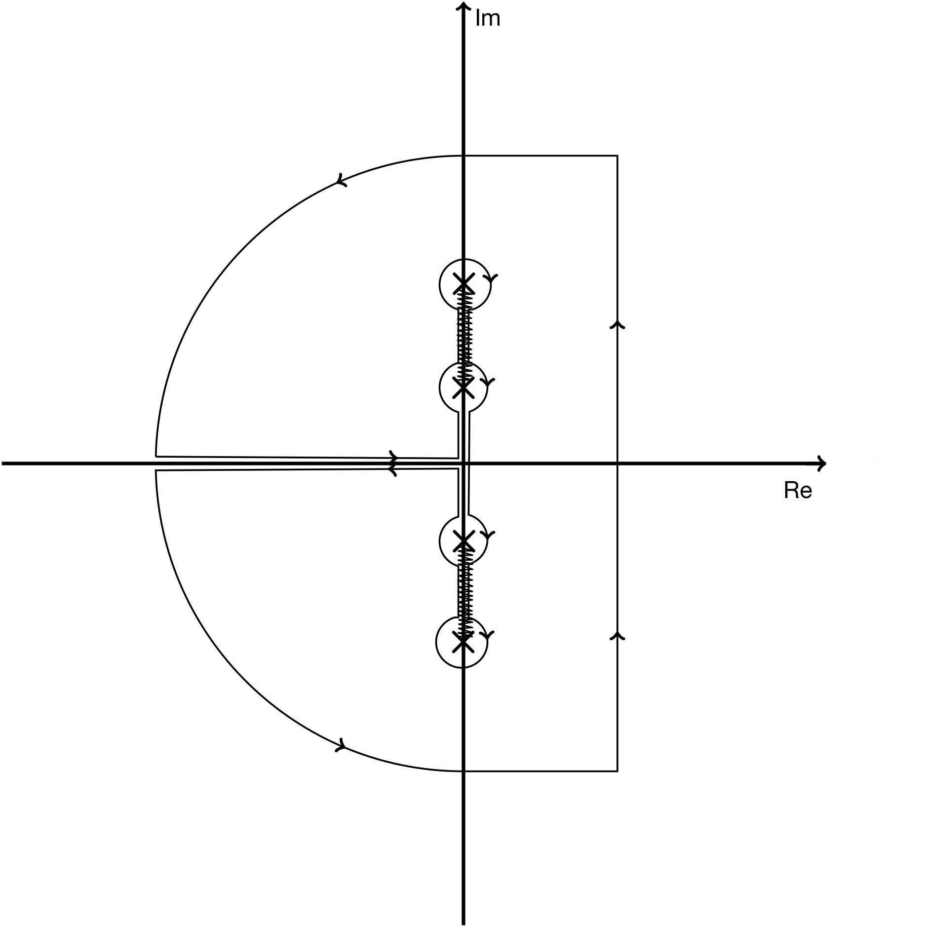
Figure 3: Illustration of the computation of the inverse Laplace transform of the fixed point kernel from Eq. (71). By definition this is the integral over a vertical path far enough to the right in the complex plane. Moving the path to the left part of the complex plane one picks up branch cut contributions determined in the text

The kernel $\tilde{k}_{I}(\lambda)$ is analytic everywhere except in the neighbourhood of points where the argument of the square root vanishes. These points are at

$$i\lambda_{\pm\pm}=\pm i\sqrt{\omega^{2}\pm\sqrt{8(n-1)}C/m}$$ (72)

The arguments of the outer square root in above is positive, hence the four points all lie on the imaginary axis. The kernel $\tilde{k}_{I}(\lambda)$ is analytic around the real line as well as for large enough $\lambda$. The contour therefore needs to encircle two cuts between respectively $i(\lambda_{+-},\lambda_{++})$ and $i(\lambda_{--},\lambda_{-+})=i(-\lambda_{++},-\lambda_{+-})$.

It is convenient to re-write the square root in (70) as $\sqrt{(\lambda^{2}+\lambda^{2}_{+-})(\lambda^{2}+\lambda^{2}_{++})}$. On the imaginary axis the argument of the square root is then positive for $z<\lambda_{+-}$, negative in the interval $(\lambda_{+-},\lambda_{++})$, and positive again for $z>\lambda_{++}$. The phase of the square root is zero on the imaginary axis up to just below the start of the cut at $i\lambda_{+-}$. Along the cut and just to the right the absolute value of the square root is $\sqrt{(z^{2}-\lambda^{2}_{+-})(-z^{2}+\lambda^{2}_{++})}$ and the phase is $i$. At the same point along the cut and just to the left the phase is $-i$. The value of the integral encircling $(\lambda_{+-},\lambda_{++})$ in the counter-clockwise direction is hence

($$+ = \int_{\lambda_{+-}}^{\lambda_{++}}e^{iz\tau}\,(2i)(-\frac{1}{2})\sqrt{(z^{2}-\lambda^{2}_{+-})(-z^{2}+\lambda^{2}_{++})},d(iz)$$)-side (73)

where $-\frac{1}{2}$ is the pre-factor of the square root in (70).

For the integral encircling $(\lambda_{--},\lambda_{-+})$ one can start from that the phase of the square root must be zero on the imaginary axis just above the cut. Along the cut and just to the left the phase is $+i$, and to the right it is $-i$. The value of this integral, encircling this cut in the positive direction, is thus

($$- = \int_{-\lambda_{++}}^{-\lambda_{+-}}e^{iz\tau}\,(-2i)(-\frac{1}{2})\sqrt{(z^{2}-\lambda^{2}_{+-})(-z^{2}+\lambda^{2}_{++})},d(iz)$$)-side (74)

$$= \int_{\lambda_{+-}}^{\lambda_{++}}e^{-iz\tau}\,(-2i)(-\frac{1}{2})\sqrt{(z^{2}-\lambda^{2}_{+-})(-z^{2}+\lambda^{2}_{++})},d(iz)$$

Combining both integrals and bringing out a dimensional factors we have a rather simple integral representation

$$k_{I}(\tau)=\Lambda\int_{q}^{1}\sin(\lambda_{++}x\tau)\sqrt{(x^{2}-q^{2})(1-x^{2})}\,dx$$ (75)

where $\Lambda=m\lambda^{3}_{++}/\pi$, and where we have used $q=\frac{\lambda_{+-}}{\lambda_{++}}$. The expression in (75) is analogous to the Mehler–Sonine representation of the Bessel function $J_{0}(\omega t)$, which is in fact nothing but the inverse Laplace transform of the function $\frac{1}{\sqrt{\Lambda^{2}+\omega^{2}}}$.

The representation (75) lends itself to a physical interpretation as follows. The total Hamiltonian in the tree subtended from $j$ will have normal modes. The kernel of the real Feynman-Vernon action on $i$ is according to the general formula

$$k_{I}(\tau)=\int d\omega\sin\omega\tau J(\omega)\,d\omega$$ (76)

where $J(\omega)$ is the spectral density. Comparing (75) and (76) we have the non-trivial result

$$J(\omega)=\left\{\begin{array}[]{ll}\sqrt{(\omega^{2}-\lambda_{+-}^{2})(\lambda_{++}^{2}-\omega^{2})}&\hbox{for $\omega\in[\lambda_{++},\lambda_{+-}]$}\\ 0&\hbox{otherwise}\\ \end{array}\right.$$

In other words, the infinite network as to its influence on one system, behaves for this ferromagnetic harmonic oscillator example as a bath with compact spectral support.

The Fourier transform of the function $k_{I}(\tau)$ in (76), when the value is zero for negative $\tau$, is the Laplace transform of $k_{I}(\tau)$ of argument $\i\nu$. Since $\hat{k}_{I}(-\nu)=\left(\hat{k}_{I}(\nu)\right)^{*}$ it is enough to consider positive $\nu$. The function $k_{I}(i\nu)$ is hence real except on the cut-line (on positive imaginary $\lambda$ axis) where it is

$$\hat{k}_{I}^{*}(\nu) = m\frac{-\nu^{2}+\omega^{2}}{4}\left(1-i\sqrt{\frac{4(n-1)\,C^{2}}{m^{2}(-\nu^{2}+\omega^{2})^{2}}-1}\right)$$

The Fourier transform of a real function satisfies $\hat{k}_{I}^{*}(-\nu)=(\hat{k}_{I}^{*}(\nu))^{*}$. We can th We note for further reference that on the cut-lines we have

$$\hat{k}_{I}^{*}(\nu)\hat{k}_{I}^{*}(-\nu) = \left(m\frac{-\nu^{2}+\omega^{2}}{4}\right)^{2}\frac{8(n-1)\,C^{2}}{m^{2}(-\nu^{2}+\omega^{2})^{2}}=\frac{(n-1)\,C^{2}}{2}$$ (77)

Note that the cavity kernels $\hat{k}_{I}^{*}(\nu)$ are of the Belief Propagation $n$-type messages (variables to interactions).

IX Iteration of the real kernel

In this section we analyze the coefficient of the linear transformation $\mathcal{W}$ in the uniform network. It is convenient to do this in the Fourier domain. From Eq. (60) one finds

$$\hat{k}_{R}^{j\rightarrow i}(\nu) = \frac{4}{C^{2}}|\hat{k}_{I}^{j\rightarrow i}(\nu)|^{2}k_{R}^{j\rightarrow i\;*}(\nu)(n-1)$$ (78)

The cavity kernels $k_{I}$ that appear here are of the Belief Propagation $m$-type (interactions to variables). At the uniform fixed point they are $(n-1)^{-1}$ times the Belief Propagation $n$-type messages which appear in (77). Combining everything we have the rather simple result

$$\frac{4}{C^{2}}|\hat{k}_{I}^{j\rightarrow i}(\nu)|^{2}=2$$ (79)

Asymptotically all Fourier components of $k_{R}$ corresponding to the spectrum of the equivalent environment grow under the iteration (multiplier is two). On the other hand it is easy to see that other Fourier components sufficiently far from the spectrum decay (multiplier less than one).

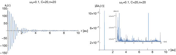
Figure 4: Numerical comparison of the two formulas for the inverse Laplace transform of the imaginary kernel Eq. (71) and Eq. (75). In the left panel the two formulas are plotted together. In the right panel absolute value of the difference between the two formulas (note a different scale in the inset). The parameters used to compute the kernels are The parameters are: $\omega_{0}=0.1$, $C=20$, $n=20$, $m=\frac{1}{2}$.. Extensive numerical comparison of the two formulas for different set of parameters allows to conclude that they are the same.

X Stability Analysis of the deterministic Replica Symmetric solution for ferromagnetic model on $n$-regular random graphs

In this section we consider the stability of the fixed point found in Section II of the main paper, in the context of Replica Symmetry. We hence here consider parameters such that the fixed point exists. The starting point is then that $k$ and $\tilde{k}$ in that analysis are not values but arguments of probability distributions that satisfy compatibility conditions. The goal is to check whether Dirac delta distributions are stable solutions of these compatibility conditions. We thus start from the BP update equations for Feynman-Vernon kernels in Laplace transform picture written as

$$Q(k)=\int\prod_{k}^{n-1}d\hat{k}_{j}P(\hat{k}_{j})\delta(k-\sum_{j}\hat{k}_{j})$$ (80)

and

$$P(\hat{k})=\int dkQ(k)\delta(\hat{k}-f_{\lambda}(k))$$ (81)

where $f_{\lambda}(k)=\frac{C^{2}}{2}\frac{G_{0}(\lambda)}{1-G_{0}(\lambda)k}\big{]}$ to be expanded around $k=k_{0}=(n-1)k^{*}$ is the Vernon transform applied to Laplace transform variable with parameter $\lambda$. $G_{0}(\lambda)=\frac{3}{m}\frac{1}{\lambda^{2}+\omega^{2}}$ is twice the response function of the free harmonic oscillator.

Instead of taking $P$ and $Q$ delta functions we then assume $P(\hat{k})\sim e^{-\frac{1}{2\sigma^{2}}(\hat{k}-k^{*})^{2}}$ That from (80) leads directly to:

$$Q(k)\sim e^{-\frac{1}{2\sigma^{2}(n-1)}(k-(n-1)k^{*})^{2}}$$ (82)

The point now is to check, whether this is consistent with a new Gaussian $P(\hat{k})$. This is clearly not the case for general $f_{\lambda}(k)$. Therefore a reasonable approach is to check if for $\sigma$ small enough, the variance of $P(\hat{k})$ grows or goes to zero. In the second case, we say that the deterministic solution $k^{*}$ (80) and (81) is stable. Otherwise, it is not.

We then proceed to estimate $\langle\hat{k}^{\alpha}\rangle$, which in practice translates into solving the following integral:

$$\langle\hat{k}^{\alpha}\rangle = \int d\hat{k}^{\alpha}\int dkQ(k)\delta(\hat{k}-f_{\lambda}(k))=$$

$$\int dkQ(k)f_{\lambda}(k)^{\alpha} = \int dke^{-\frac{1}{2\sigma^{2}(n-1)}(k-(n-1)k^{*})^{2}}f_{\lambda}(k)^{\alpha}$$

We expand the function $f_{\lambda}(k)^{\alpha}=\big{[}\frac{C^{2}}{2}\frac{G_{0}(\lambda)}{1-G_{0}(\lambda)k}\big{]}^{\alpha}$ around $k=k_{0}=(n-1)k^{*}$. For the expected value ($\alpha=1$) we have

$$\frac{G_{0}(\lambda)}{1-G_{0}(\lambda)k} = \frac{G_{0}(\lambda)}{1-G_{0}(\lambda)k_{0}}+\big{[}\frac{G_{0}(\lambda)}{1-G_{0}(\lambda)k_{0}}\big{]}^{2}(k-k_{0})+\big{[}\frac{G_{0}(\lambda)}{1-G_{0}(\lambda)k_{0}}\big{]}^{3}(k-k_{0})^{2}$$ (83)

such that

$$\langle k\rangle = \frac{C^{2}}{2}\Big{[}\frac{G_{0}(\lambda)}{1-G_{0}(\lambda)k_{0}}\int dke^{-\frac{1}{2\sigma^{2}(n-1)}(k-k_{0})^{2}}+\big{(}\frac{G_{0}(\lambda)}{1-G_{0}(\lambda)k_{0}}\big{)}^{3}\int dke^{-\frac{1}{2\sigma^{2}(n-1)}(k-k_{0})^{2}}(k-k_{0})^{2}\Big{]}=$$

$$= \frac{C^{2}}{2}\frac{G_{0}(\lambda)}{1-G_{0}(\lambda)k_{0}}\Big{[}1+\sigma^{2}(n-1)\big{(}\frac{G_{0}(\lambda)}{1-G_{0}(\lambda)k_{0}}\big{)}^{2}\Big{]}$$

Similarly, for the second moment ($\alpha=2$):

$$\left[\frac{G_{0}(\lambda)}{1-G_{0}(\lambda)k}\right]^{2} = \left[\frac{G_{0}(\lambda)}{1-G_{0}(\lambda)k_{0}}\right]^{2}+2\left[\frac{G_{0}(\lambda)}{1-G_{0}(\lambda)k_{0}}\right]^{3}(k-k_{0})+\frac{6}{2}\left[\frac{G_{0}(\lambda)}{1-G_{0}(\lambda)k_{0}}\right]^{4}(k-k_{0})^{2}$$ (85)

and

$$\langle k^{2}\rangle = \frac{C^{4}}{4}\big{[}\frac{G_{0}(\lambda)}{1-G_{0}(\lambda)k_{0}}\big{]}^{2}\Big{[}1+3\sigma^{2}(n-1)\big{[}\frac{G_{0}(\lambda)}{1-G_{0}(\lambda)k_{0}}\big{]}^{2}\Big{]}$$ (86)

Putting everything together we have

$$\langle k^{2}\rangle-\langle k\rangle^{2} = \sigma^{2}\frac{(n-1)}{4}$$ (87)

$$\quad C^{4}\big{[}\frac{G_{0}(\lambda)}{1-G_{0}(\lambda)k_{0}}\big{]}^{4}$$

The variance of the distribution after passing through the BP update is hence proportional to original variance $\sigma^{2}$. Note that the combination $C\frac{G_{0}(\lambda)}{1-G_{0}(\lambda)k_{0}}$ is dimension-less, and that $\sigma$ has the same dimension as $k$.

Since we expand around the fixed point $k^{*}$ we have $k_{0}=(n-1)k^{*}$, $\frac{G_{0}(\lambda)}{1-G_{0}(\lambda)k_{0}}=\frac{2}{C^{2}(n-1)}k^{*}$ and $k^{*}=m\frac{\lambda^{2}+\omega^{2}}{4}\left(1-\sqrt{1-\frac{8(n-1)\,C^{2}}{m^{2}(\lambda^{2}+\omega^{2})^{2}}}\right)$. For small $C$ we can neglect the difference between $\omega$ and $\omega_{0}$ and have

$$k^{*}\approx\frac{(n-1)\,C^{2}}{m(\lambda^{2}+\omega_{0}^{2})}\quad\hbox{($C$ small)}$$ (88)

and hence

$$\frac{G_{0}(\lambda)}{1-G_{0}(\lambda)k_{0}}\approx\frac{1}{(\lambda^{2}+\omega_{0}^{2})}\quad\hbox{($C$ small)}$$ (89)

For small values of $C$ the proportionality is hence less than one, and by iteration the Gaussian gets sharper. This means that the deterministic (delta-function) solution is stable.

References

- Mézard and Montanari (2009) M. Mézard and A. Montanari, Information, Physics and Computation (Oxford University Press, 2009).
- Richardson and Urbanke (2008) T. Richardson and R. Urbanke, Modern Coding Theory (Cambridge University Press, 2008).
- Wainwright and Jordan (2008) M. J. Wainwright and M. I. Jordan, Found. Trends Mach. Learn. 1, 1–305 (2008), ISSN 1935-8237, URL https://doi.org/10.1561/2200000001.
- Bethe and Bragg (1935) H. A. Bethe and W. L. Bragg, Proceedings of the Royal Society of London. Series A - Mathematical and Physical Sciences 150, 552 (1935), eprint https://royalsocietypublishing.org/doi/pdf/10.1098/rspa.1935.0122, URL https://royalsocietypublishing.org/doi/abs/10.1098/rspa.1935.0122.
- Yedidia et al. (2003) J. S. Yedidia, W. T. Freeman, and Y. Weiss, Understanding Belief Propagation and Its Generalizations (Morgan Kaufmann Publishers Inc., San Francisco, CA, USA, 2003), p. 239–269, ISBN 1558608117.
- Abou-Chacra et al. (1973) R. Abou-Chacra, D. J. Thouless, and P. W. Anderson, Journal of Physics C: Solid State Physics 6, 1734 (1973), URL https://doi.org/10.1088%2F0022-3719%2F6%2F10%2F009.
- Dupont et al. (2020) M. Dupont, N. Laflorencie, and G. Lemarié, Dirty bosons on the cayley tree: Bose-einstein condensation versus ergodicity breaking (2020).
- Parisi et al. (2019) G. Parisi, S. Pascazio, F. Pietracaprina, V. Ros, and A. Scardicchio, Journal of Physics A: Mathematical and Theoretical 53, 014003 (2019), URL https://doi.org/10.1088%2F1751-8121%2Fab56e8.
- García-Mata et al. (2020) I. García-Mata, J. Martin, R. Dubertrand, O. Giraud, B. Georgeot, and G. Lemarié, Phys. Rev. Research 2, 012020 (2020), URL https://link.aps.org/doi/10.1103/PhysRevResearch.2.012020.
- Laumann et al. (2008) C. Laumann, A. Scardicchio, and S. L. Sondhi, Phys. Rev. B 78, 134424 (2008), URL https://link.aps.org/doi/10.1103/PhysRevB.78.134424.
- Bapst et al. (2013) V. Bapst, L. Foini, F. Krzakala, G. Semerjian, and F. Zamponi, Physics Reports 523, 127 (2013), ISSN 0370-1573, the Quantum Adiabatic Algorithm Applied to Random Optimization Problems: The Quantum Spin Glass Perspective, URL http://www.sciencedirect.com/science/article/pii/S037015731200347X.
- Hastings (2007) M. B. Hastings, Phys. Rev. B 76, 201102 (2007), URL https://link.aps.org/doi/10.1103/PhysRevB.76.201102.
- Leifer and Poulin (2008) M. Leifer and D. Poulin, Annals of Physics 323, 1899 (2008), ISSN 0003-4916, URL http://www.sciencedirect.com/science/article/pii/S0003491607001509.
- Poulin and Bilgin (2008) D. Poulin and E. Bilgin, Phys. Rev. A 77, 052318 (2008), URL https://link.aps.org/doi/10.1103/PhysRevA.77.052318.
- Ioffe and Mézard (2010) L. B. Ioffe and M. Mézard, Phys. Rev. Lett. 105, 037001 (2010), URL https://link.aps.org/doi/10.1103/PhysRevLett.105.037001.
- Dimitrova and Mézard (2011) O. Dimitrova and M. Mézard, Journal of Statistical Mechanics: Theory and Experiment 2011, P01020 (2011), URL https://doi.org/10.1088%2F1742-5468%2F2011%2F01%2Fp01020.
- Loeliger and Vontobel (2017) H. Loeliger and P. O. Vontobel, IEEE Transactions on Information Theory 63, 5642 (2017).
- Renes (2017) J. M. Renes, New Journal of Physics 19, 072001 (2017), URL https://doi.org/10.1088%2F1367-2630%2Faa7c78.
- Feynman and Vernon (1963) R. P. Feynman and J. Vernon, F. L., Annals of Physics 24, 118 (1963).
- Beals et al. (2013) R. Beals, S. Brierley, O. Gray, A. W. Harrow, S. Kutin, N. Linden, D. Shepherd, and M. Stather, Proc. R. Soc. A. 469, 20120686 (2013).
- Boixo et al. (2018) S. Boixo, S. V. Isakov, V. N. Smelyanskiy, R. Babbush, N. Ding, Z. Jiang, M. J. Bremner, J. M. Martinis, and H. Neven, Nature Physics 14, 595 (2018).
- Cross et al. (2019) A. W. Cross, L. S. Bishop, S. Sheldon, P. D. Nation, and J. M. Gambetta, Phys. Rev. A 100, 032328 (2019), URL https://link.aps.org/doi/10.1103/PhysRevA.100.032328.
- Nam and Maslov (2019) Y. Nam and D. Maslov, npj Quantum Information 5, 44 (2019).
- Das and Chakrabarti (2008) A. Das and B. K. Chakrabarti, Rev. Mod. Phys. 80, 1061 (2008), URL https://link.aps.org/doi/10.1103/RevModPhys.80.1061.
- Neri and Bollé (2009) I. Neri and D. Bollé, Journal of Statistical Mechanics: Theory and Experiment 2009, P08009 (2009), URL https://doi.org/10.1088%2F1742-5468%2F2009%2F08%2Fp08009.
- Aurell and Mahmoudi (2011) E. Aurell and H. Mahmoudi, Journal of Statistical Mechanics: Theory and Experiment 2011, P04014 (2011), URL https://doi.org/10.1088%2F1742-5468%2F2011%2F04%2Fp04014.
- Aurell and Mahmoudi (2012) E. Aurell and H. Mahmoudi, Phys. Rev. E 85, 031119 (2012), URL https://link.aps.org/doi/10.1103/PhysRevE.85.031119.
- Del Ferraro and Aurell (2015) G. Del Ferraro and E. Aurell, Phys. Rev. E 92, 010102 (2015), URL https://link.aps.org/doi/10.1103/PhysRevE.92.010102.
- Barthel et al. (2018) T. Barthel, C. De Bacco, and S. Franz, Phys. Rev. E 97, 010104 (2018), URL https://link.aps.org/doi/10.1103/PhysRevE.97.010104.
- Barthel (2020) T. Barthel, Journal of Statistical Mechanics: Theory and Experiment 2020, 013217 (2020), URL https://doi.org/10.1088%2F1742-5468%2Fab5701.
- Aurell et al. (2017) E. Aurell, G. Del Ferraro, E. Domínguez, and R. Mulet, Phys. Rev. E 95, 052119 (2017), URL https://link.aps.org/doi/10.1103/PhysRevE.95.052119.
- Aurell et al. (2018) E. Aurell, E. Domínguez, D. Machado, and R. Mulet, Phys. Rev. E 97, 050103 (2018), URL https://link.aps.org/doi/10.1103/PhysRevE.97.050103.
- Aurell et al. (2019) E. Aurell, E. Domínguez, D. Machado, and R. Mulet, Phys. Rev. Lett. 123, 230602 (2019), URL https://link.aps.org/doi/10.1103/PhysRevLett.123.230602.
- Vernon (1959) F. L. Vernon, Ph.D. thesis, California Institute of Technology (1959), URL https://resolver.caltech.edu/CaltechETD:etd-02242006-154616.
- Aurell and Tuziemski (2021) E. Aurell and J. Tuziemski, The vernon transform and its use in quantum thermodynamics, arXiv:2103.13255 (2021).
- Miller and Derrida (1994) J. D. Miller and B. Derrida, Journal of Statistical Physics 75, 357 (1994).
- Aurell et al. (2020) E. Aurell, R. Kawai, and K. Goyal, Journal of Physics A: Mathematical and Theoretical 53, 275303 (2020), URL https://doi.org/10.1088%2F1751-8121%2Fab9274.
- Sudderth et al. (2003) E. B. Sudderth, A. T. Ihler, W. T. Freeman, and A. S. Willsky, in 2003 IEEE Computer Society Conference on Computer Vision and Pattern Recognition, 2003. Proceedings. (2003), vol. 1, pp. I–I.
- Bickson et al. (2009) D. Bickson, A. T. Ihler, H. Avissar, and D. Dolev, in 2009 47th Annual Allerton Conference on Communication, Control, and Computing (Allerton) (2009), pp. 439–446.
- GR (2014) in Table of Integrals, Series, and Products (Eighth Edition), edited by D. Zwillinger, V. Moll, I. Gradshteyn, and I. Ryzhik (Academic Press, Boston, 2014), pp. 1077–1103, eighth edition ed., ISBN 978-0-12-384933-5, URL https://www.sciencedirect.com/science/article/pii/B9780123849335000126.