Periodicity of limit cycles in a max-plus dynamical system

Abstract

By introducing a max-plus dynamical system having limit cycles, we discuss their periodicity, especially the number of discrete states in them. We also find that quasi-periodic cycles exist depending on the bifurcation parameter in the system. Approximate relations between the number of states in the limit cycles and the value of the bifurcation parameter are proposed.

For nonlinear and nonequilibrium phenomena, their description based on max-plus algebra has been made. Soliton behaviors in integrable systems [1], reaction-diffusion dynamics in dissipative systems [2, 3], and bifurcation phenomena in dynamical systems [4, 5] are typical examples. Max-plus equations can be derived from discrete difference equations through ultradiscretization[1]. They can be also obtained from continuous differential equations by appropriate discretization such as tropical discretization[3]. The crucial point is that there are cases where max-plus description can retain and elucidate essential dynamical structures of the original discrete or continuous systems.

Recently, we have derived the following max-plus dynamical system from the tropically discretized Sel’kov model via ultradiscretization[5]:

$$\begin{cases}\;X_{n+1}&=Y_{n}+\max(0,2X_{n}),\\ \;Y_{n+1}&=B-\max(0,2X_{n}).\end{cases}$$ (1)

We found that eq.(1) has two limit cycles, $C$ and $C_{s}$, with period seven when $B>0$; they possess different basins. The difference between them is that $C$ has points in the region $X_{n}\leq 0$ and $Y_{n}\leq 0$, but $C_{s}$ does not. So far, understanding the periodicity of these limit cycles is not sufficient. For example, it is not clear how the number of discrete states in the limit cycles is determined. In this letter, we discuss such a unclear point by focusing on $C$. In eq.(1), we can perform the variable transformation, $X_{n}/B\rightarrow X_{n}$ and $Y_{n}/B\rightarrow Y_{n}$, without essential change of its dynamical properties for positive $B$. In other words, we can set $B=1$ in eq.(1) without loss of generality if only $B>0$ is treated. Then we consider the following set of equations hereafter:

$$\begin{cases}\;X_{n+1}&=Y_{n}+\max(0,RX_{n}),\\ \;Y_{n+1}&=1-\max(0,RX_{n}).\end{cases}$$ (2)

Eq.(2) possesses a new parameter $R(>0)$ and is considered as a generalization of eq.(1) with $B>0$.

Now we consider dynamical properties of eq.(2) by dividing $(X_{n},Y_{n})$ plane into the three regions I ($X_{n}>0$), II-1 ($X_{n}\leq 0,Y_{n}\leq 0$), and II-2 ($X_{n}\leq 0,Y_{n}>0$). In region I, eq.(2) is represented by the matrix form,

$$\bm{x}_{n+1}=\left(\begin{array}[]{ccc}R&1\\ -R&0\\ \end{array}\right)\bm{x}_{n}+\left(\begin{array}[]{ccc}0\\ 1\end{array}\right),$$ (3)

where $\bm{x}_{n}=\left(\begin{array}[]{c}X_{n}\\ Y_{n}\end{array}\right)$. $R$ dependence of dynamical properties of eq.(3) is understood as follows[6]. For the matrix $A=\left(\begin{array}[]{ccc}R&1\\ -R&0\\ \end{array}\right)$, trace and determinant of $A$ are $\mathrm{tr}A=\mathrm{det}A=R$. Figure 1 shows a typical diagram for the two dimensional dynamics $\bm{x}_{n+1}=A\bm{x}_{n}$ in terms of $\mathrm{tr}A$ and $\mathrm{det}A$.

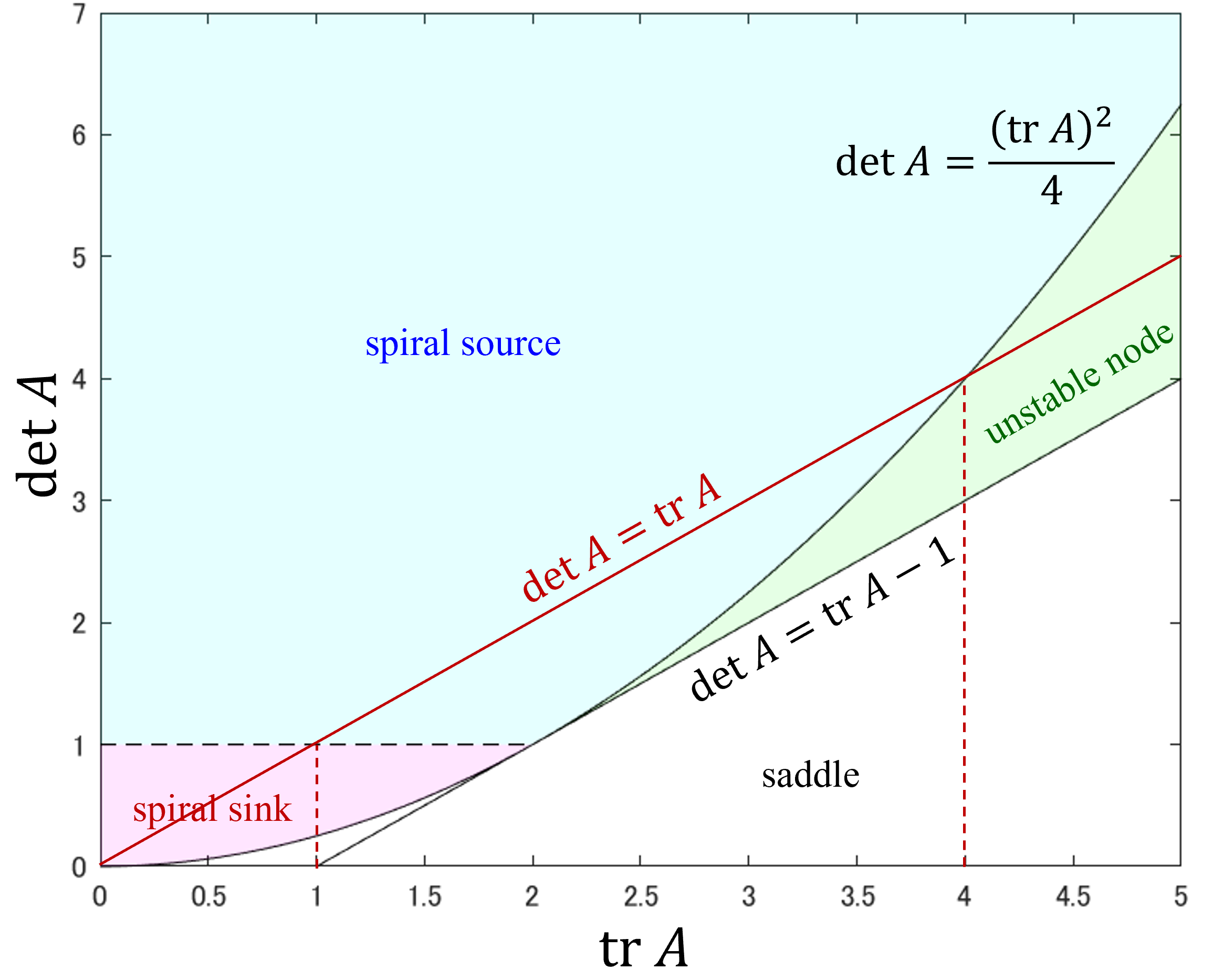
Figure 1: A diagram for dynamics of the discrete linear dynamical system $\bm{x}_{n+1}=A\bm{x}_{n}$ in two dimensions.

It is found that the dynamical properties of eq.(3) depend on $R$ along the line $\mathrm{tr}A=\mathrm{det}A$. From this figure, if limit cycles exist, $R$ is in the region $1<R<4$, where the fixed point of eq.(3) becomes clockwise spiral source. Then there is a case for $1<R<4$ where a state (point) in region I finally gets into region II-1 during time evolution of $\bm{x}_{n}$ by eq.(3). Furthermore, any state in region II-1, $X_{0}\leq 0$ and $Y_{0}\leq 0$, changes as $(X_{0},Y_{0})\rightarrow(Y_{0},1)\rightarrow(1,1)$ from eq.(2). The state $(1,1)$ is in region I, then there exists a cycle having the state $(1,1)$ when $1<R<4$. Therefore, $R$ is considered as the bifurcation parameter for Neimark-Sacker bifurcation (Hopf bifurcation for discrete dynamical systems), which occurs at $R=1$. Figure 2 shows trajectories for two different case of $R$: (a) $R=0.5$, (b) $R=1.5$. We can interpret this max-plus equation as describing a reset event from $(X_{0},Y_{0})$ to $(1,1)$ when the value of $X_{n}$ becomes negative; the value ‘0’ in the term $\max(0,RX_{n})$ is considered as the threshold for $X_{n}$.

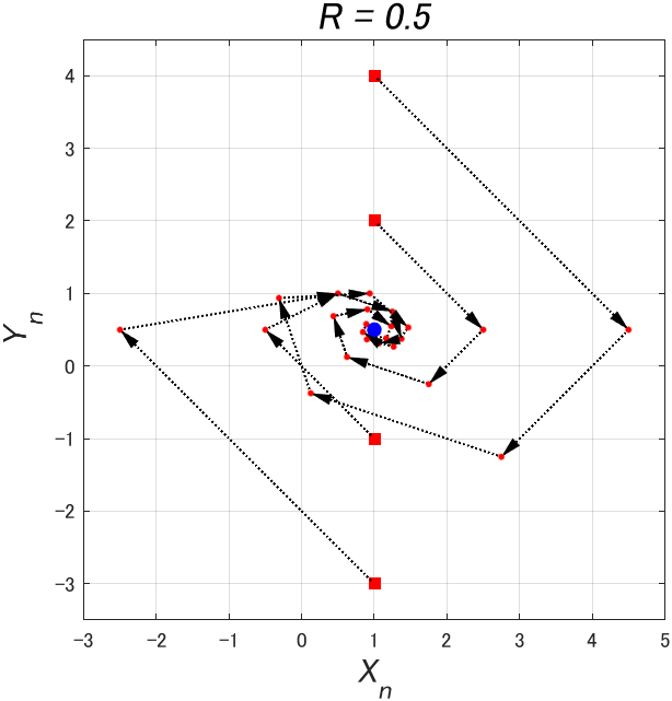
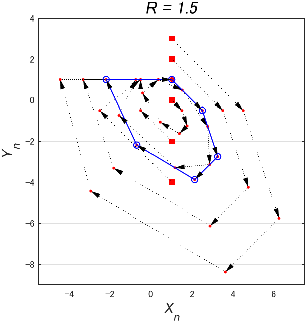
(a)                                                              (b)

Figure 2: Examples of trajectories starting from red squares. (a) $R=0.5$. The blue point shows (1, 1/2) which is the stable fixed point. (b) $R=1.5$. The blue cycle shows the limit cycle $C$ with period six.

Since it takes two steps to reach the state $(1,1)$ from any point in region II-1, the period of the limit cycle is $n+2$ where $n$ is the number of states in region I. Actually, the previous study[5] shows $n=5$ for $R=2$, then the period of the limit cycle is 7. Here we consider time evolution of eq.(3) in region I starting from the initial state $\bm{x}_{0}=\left(\begin{array}[]{c}1\\ 1\end{array}\right)$. Eq.(3) is formally solved as

$$\bm{x}_{n}=A^{n}\bm{x}_{0}+\left(1-A^{n}\right)\left(1-A\right)^{-1}\bm{b}.$$ (4)

Denoting $\bm{x}_{n}=\left(\begin{array}[]{c}G_{X}(n,R)\\ G_{Y}(n,R)\end{array}\right)$ as the solution of eq.(4) by setting $A=\left(\begin{array}[]{ccc}R&1\\ -R&0\\ \end{array}\right)$, $\displaystyle\bm{b}=\left(\begin{array}[]{c}0\\ 1\end{array}\right)$, and $\bm{x}_{0}=\left(\begin{array}[]{c}1\\ 1\end{array}\right)$, $G_{X}(n,R)$ and $G_{Y}(n,R)$ are explicitly given as

$$G_{X}(n,R) = 1+\frac{R^{\frac{n+1}{2}}}{2^{n}i\sqrt{4-R}}\biggl{\{}\left(\sqrt{R}+i\sqrt{4-R}\right)^{n}-\left(\sqrt{R}-i\sqrt{4-R}\right)^{n}\biggr{\}},$$ (5)

$$G_{Y}(n,R) = 1-R+\frac{R^{\frac{n+1}{2}}}{2^{n+1}}\Biggl{[}\biggl{\{}\left(\sqrt{R}+i\sqrt{4-R}\right)^{n}+\left(\sqrt{R}-i\sqrt{4-R}\right)^{n}\biggr{\}}$$ (6)

$$-\frac{1}{i}\sqrt{\frac{R}{4-R}}\biggl{\{}\left(\sqrt{R}+i\sqrt{4-R}\right)^{n}-\left(\sqrt{R}-i\sqrt{4-R}\right)^{n}\biggr{\}}\Biggr{]},$$

$(1<R<4)$. We note that the following relation holds between $G_{X}$ and $G_{Y}$,

$$RG_{X}(n-1,R)+G_{Y}(n,R)=1.$$ (7)

Based on eqs.(5) and (6), the number of states in region I of the limit cycle is given by the minimum $n$ satisfying $G_{X}(n,R)\leq 0$ and $G_{Y}(n,R)\leq 0$ for a fixed $R$, which means $\bm{x}_{n}$ is in region II-1. Figure 3 shows the contour plots of $G_{X}(n,R)$ and $G_{Y}(n,R)$.

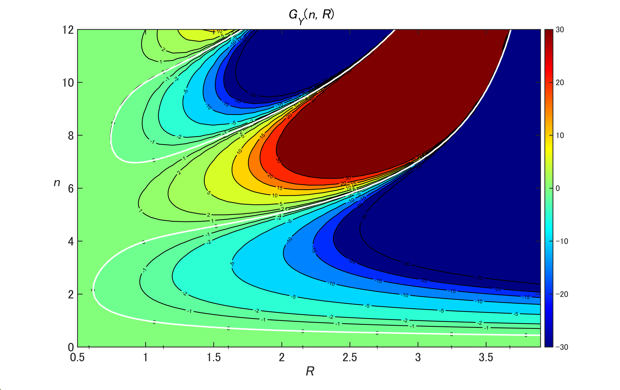
(a)                                                                (b)

Figure 3: Contour plots of (a) $G_{X}(n,R)$ and (b) $G_{Y}(n,R)$. The white curves show the relations of (a) $G_{X}(n,R)=0$ and (b) $G_{Y}(n,R)=0$.

Figure 4 shows the curves for $G_{X}(n,R)=0$ and $G_{Y}(n,R)=0$, which are depicted as white curves in Fig.3.

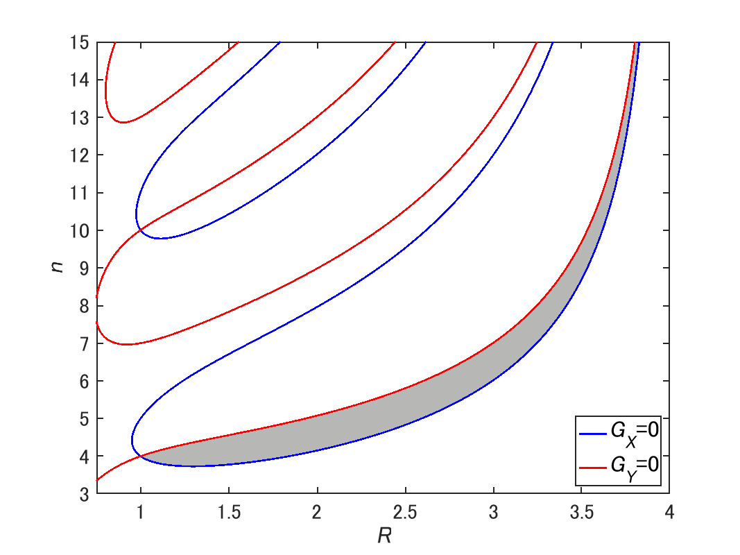
Figure 4: The curves for $G_{X}(n,R)=0$ and $G_{Y}(n,R)=0$. The gray region shows the condition for existence of limit cycles.

It is found from the signs of $G_{X}$ and $G_{Y}$ shown in Fig.3 that the limit cycles can emerge with $(n,R)$ in the gray region of Fig.4. Now we determine the region of $R$ satisfying $G_{X}(n,R)\leq 0$ and $G_{Y}(n,R)\leq 0$ for a given $n$. When we express the solution of $G_{X}(n,R)=0$ and $G_{Y}(n,R)=0$ with respect to $R$ as $R_{X}(n)$ and $R_{Y}(n)$, the region of $R$ for existence of the limit cycle with period $n+2$ is $R_{Y}(n)\leq R\leq R_{X}(n)$. Table 1 shows the numerical results of such regions as a function of $n$.

Table 1: Numerically obtained regions of $R$ for existence of limit cycles with period $n+2$, where $n$ is the number of states in region I of the cycles.

$n$	period($=n+2$)	$R_{Y}(n)\leq R\leq R_{X}(n)$
4	6	1.000000$\cdots$ $\sim$ 1.83928$\cdots$
5	7	1.93318 $\cdots\sim$ 2.59205 $\cdots$
6	8	2.60229 $\cdots\sim$ 2.99375 $\cdots$
7	9	2.99585 $\cdots\sim$ 3.24522 $\cdots$
8	10	3.24576 $\cdots\sim$ 3.41367 $\cdots$
9	11	3.41383 $\cdots\sim$ 3.53191 $\cdots$
10	12	3.53196 $\cdots\sim$ 3.61797 $\cdots$
⋮	⋮	⋮

Table 1 shows that there are finite gaps between regions of $R$ for two limit cycles with periods $n$ and $n+1$. For example, the region $1.83928\cdots<R<1.93318\cdots$ corresponds to the gap between the two cycles with periods 6 and 7. In these gaps, $R_{X}(n)<R<R_{Y}(n+1)$, we find quasi-periodic limit cycles composed of $n$ and $n+1$ periods. Figure 5 shows the examples of the quasi-periodic cycles with $(6+7)$ period for $R=1.9$ and with $(7+8)$ period for $R=2.6$.

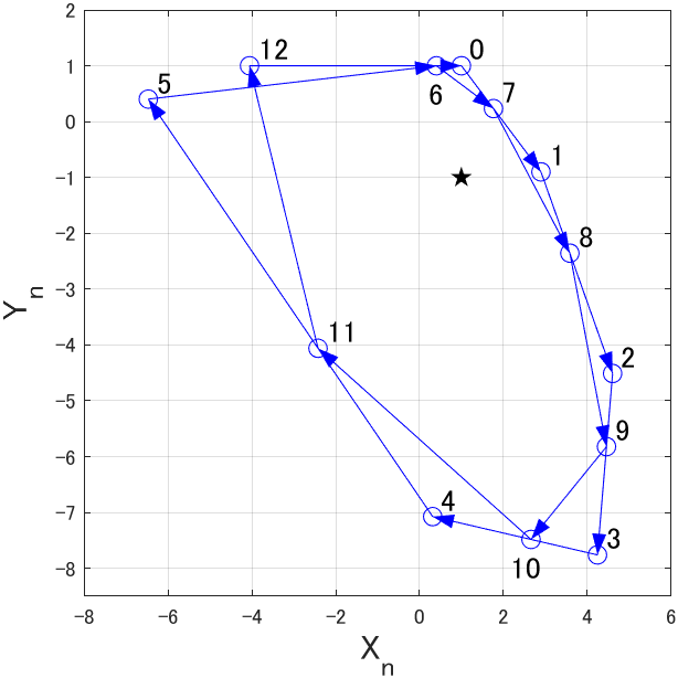
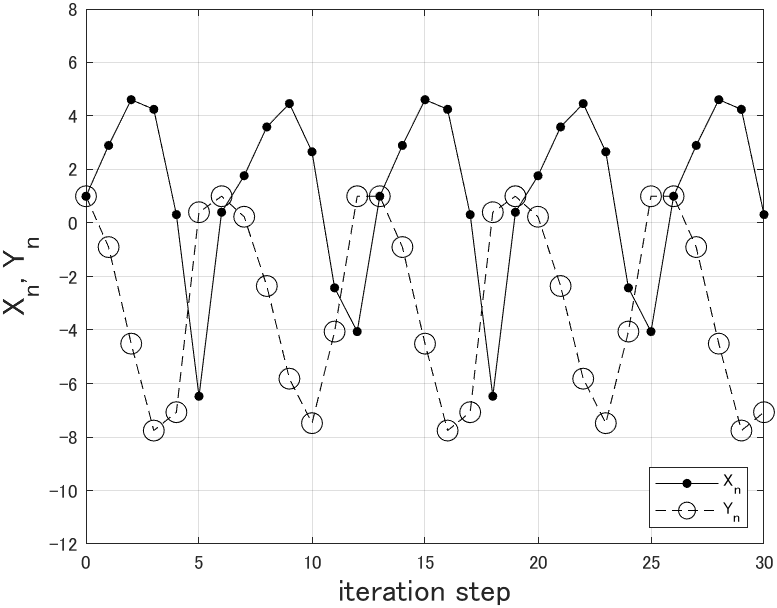
(a)                                                              (b)

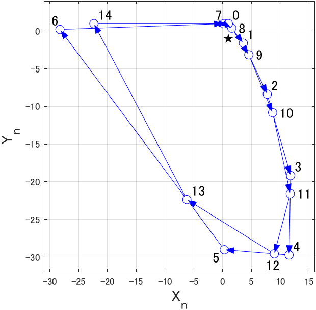
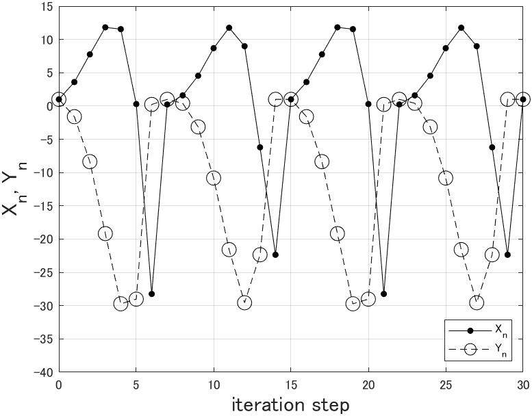
(c)                                                              (d)

Figure 5: Quasi-periodic cycles for two different values of $R$. (a) trajectory and (b) time evolution for $R=1.9$. (c) trajectory and (d) time evolution for $R=2.6$.

Existence of such quasi-periodic limit cycles seems to be due to absence of the integer $n$ in these gaps. The gaps exist between every two limit cycles with periods $n$ and $n+1$. In proof, for $R=R_{X}(n)$ which satisfies $G_{X}(n,R_{X}(n))=0$, the following relation holds from eq.(7),

$$R_{X}(n)G_{X}(n,R_{X}(n))+G_{Y}(n+1,R_{X}(n))=G_{Y}(n+1,R_{X}(n))=1.$$

Then the relation

$$G_{Y}(n+1,R_{X}(n))=1>0=G_{Y}(n+1,R_{Y}(n+1))$$

is obtained. Considering the contour plots shown in Fig.3(b), we find

$$R_{X}(n)<R_{Y}(n+1),$$

which shows existence of the finite gaps for occurrence of quasi-periodic limit cycles.

We propose several approximate relations between $n$ and $R$. In order to obtain them, the following variable transformation from $R$ to $\theta$ is considered,

$$e^{i\theta}=\frac{\sqrt{R}+i\sqrt{4-R}}{2}.$$ (8)

The range of values which $\theta$ can take is $\displaystyle 0<\theta<\frac{\pi}{3}$ because of $1<R<4$. Applying this variable transformation to eqs.(5) and (6), we obtain $G_{X}$ and $G_{Y}$ as a function of $n$ and $\theta$.

$$G_{X}(n,\theta) = 1+\frac{\left(2\cos\theta\right)^{n+1}}{\sin\theta}\sin n\theta,$$ (9)

$$G_{Y}(n,\theta) = 1-4\cos^{2}\theta+\frac{\left(2\cos\theta\right)^{n+2}}{\sin\theta}\sin(n-1)\theta,$$ (10)

($n\geq 4$). Figure 3 tells that the values of both $|G_{X}|$ and $|G_{Y}|$ rapidly increase when they move away from the curves $G_{X}=0$ and $G_{Y}=0$ especially for large $R$ (small $\theta$). Therefore, the value of $\theta$ for $G_{X}(n,\theta)=0$ can be approximated by $\theta_{X}$ satisfying $G_{X}(n,\theta_{X})=1$, namely $\sin n\theta_{X}=0$ from eq.(9). As the smallest positive $n$ for $\sin n\theta_{X}=0$, we obtain $n\theta_{X}=\pi$. In the similar way for eq.(10), we also obtain the approximate value $\theta_{Y}$ which satisfies $\sin(n-1)\theta_{Y}=0$, that is $(n-1)\theta_{Y}=\pi$. Considering the forms of $\theta_{X}$ and $\theta_{Y}$, we roughly estimate $\theta$ as $\displaystyle\left(n-\frac{1}{2}\right)\theta\approx\pi$. (The constant $\displaystyle\frac{1}{2}$ is just a candidate between 0 and 1. A better constant may be found from an appropriate fitting.) Then an approximate relation between $n$ and $\theta$ (or $R$) is obtained as

$$n\approx\frac{1}{2}+\frac{\pi}{\theta}=\frac{1}{2}+\frac{\pi}{\arccos\frac{\sqrt{R}}{2}}.$$ (11)

From the relation $\displaystyle\cos^{2}\theta=\frac{R}{4}$, $\theta$ is further approximated as $\displaystyle\theta\approx\frac{\sqrt{4-R}}{2}$ for $\theta\ll 1$ ($R\lesssim 4$). Therefore, eq.(11) can be rewritten as

$$n\approx\frac{1}{2}+\frac{2\pi}{\sqrt{4-R}}.$$ (12)

Figure 6 shows the plots of eqs.(11) and (12) together with the gray region in Fig.4. This figure shows that these two approximate relations are roughly in the gray region; these approximations are found to be well especially with larger $R$.

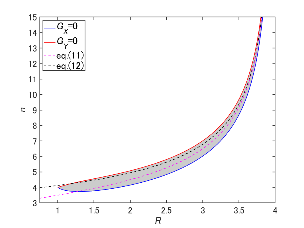
Figure 6: The two approximations given by eqs.(11) and (12). The gray region is the same as Fig.4.

In conclusion, we have discussed periodicity of the limit cycles based on eq.(2). This equation has the bifurcation parameter $R$, and the limit cycles emerge when $1<R<4$. The number of states $n$ in the limit cycles is given as a function of $R$. It is found that quasi-periodic cycles exist depending on the value of $R$. The two approximations for the relation between $n$ and $R$, i.e. eqs.(11) and (12), have been demonstrated. The present results are expected to give fundamental information for periodic phenomena with max-plus description.

Acknowledgement

The authors are grateful to Prof. T. Yamamoto, and Prof. Emeritus A. Kitada at Waseda University for encouragements. This work was supported by Sumitomo Foundation, Grant Number 200146.

References

• [1] T. Tokihiro, D. Takahashi, J. Matsukidaira, and J. Satsuma, Phys. Rev. Lett. 76, 3247 (1996).
• [2] K. Matsuya and M. Murata, Discrete Contin. Dyn. Syst. B 20 173 (2015).
• [3] M. Murata, J. Differ. Equations Appl. 19 1008 (2013).
• [4] S. Ohmori and Y. Yamazaki, J. Math. Phys. 61 122702 (2020)
• [5] S. Ohmori and Y. Yamazaki, submitted (arXiv:2107.02435).
• [6] O. Galor, Discrete Dynamical Systems (Springer, New York 2010).