Sauter-Schwinger effect for colliding laser pulses

Abstract

Via a combination of analytical and numerical methods, we study electron-positron pair creation by the electromagnetic field $\mbox{\boldmath$A$}(t,\mbox{\boldmath$r$})=[f(ct-x)+f(ct+x)]\mbox{\boldmath$e$}_{y}$ of two colliding laser pulses. Employing a generalized WKB approach, we find that the pair creation rate along the symmetry plane $x=0$ (where one would expect the maximum contribution) displays the same exponential dependence as for a purely time-dependent electric field $\mbox{\boldmath$A$}(t)=2f(ct)\mbox{\boldmath$e$}_{y}$. The pre-factor in front of this exponential does also contain corrections due to focusing or de-focusing effects induced by the spatially inhomogeneous magnetic field. We compare our analytical results to numerical simulations using the Dirac-Heisenberg-Wigner method and find good agreement.

Introduction

As one of the most striking and fundamental predictions of quantum electrodynamics (QED), the vacuum should become unstable in the presence of strong electric fields, leading to the spontaneous creation of electron-positron pairs (“matter from light”) HeisenbergEuler ; Weisskopf . For a constant electric field $E$, the pair-creation probability $P$ displays an exponential dependence ($\hbar=c=1$)

$$P\sim\exp\left\{-\pi\,\frac{m^{2}}{qE}\right\}=\exp\left\{-\pi\,\frac{E_{S}}{E}\right\}\,,$$ (1)

with the electron mass $m$ and elementary charge $q$, which can be combined to yield the Schwinger critical field $E_{S}=m^{2}/q\approx 1.3\times 10^{18}~{}\rm V/m$. The above functional dependence does not admit a Taylor expansion in $q$ which indicates that this Sauter-Schwinger effect (1) is a non-perturbative phenomenon Sauter:1931 ; Schwinger:1951nm . As a result, the corresponding calculations can be quite non-trivial and our knowledge beyond the case of constant fields is very limited PhysRevA.102.063110 ; PhysRevA.102.052805 . For slowly varying fields, we may apply the locally constant field approximation by evaluating Eq. (1), together with its generalization to additional magnetic fields, at each space-time point Nikishov . However, this approximation has a limited range of applicability and does not capture many important effects, such as the dynamically assisted Sauter-Schwinger effect DynamicallyAssistedSchwinger ; Catalysis ; OTTO2015335 ; PhysRevD.100.116018 .

From a fundamental point of view as well as in anticipation of experimental initiatives aiming at ultra-high field strengths footnote1 , it is important to better understand the Sauter-Schwinger effect for non-constant fields PhysRevLett.101.200403 ; PhysRevLett.105.220407 . While there has been progress regarding fields which depend on one coordinate (e.g., space $x$ or time $t$ KimPage ; Kleinert , or a light-cone variable $t-x$ PhysRevD.84.125022 ; Heinzl ), our understanding of more complex field dependences, e.g., the interplay between spatial and temporal variations, is still in its infancy PhysRevD.72.105004 ; PhysRevA.99.022125 . Furthermore, going from simple models towards realistic field configurations requires the consideration of transversal fields which are vacuum solutions of the Maxwell equations. In the following, we venture a step into this direction by employing a combination of analytical and numerical methods.

The model

In order to treat a potentially realistic yet simple field configuration, we consider the head-on collision of two equal plane-wave laser pulses, see also aleksandrov_prd_2017_2

$$\mbox{\boldmath$A$}(t,\mbox{\boldmath$r$})=\left[f(t-x)+f(t+x)\right]\mbox{\boldmath$e$}_{y}\,.$$ (2)

For asymmetric collision scenarios, see, e.g., Ilderton ; Fedotov ; PhysRevD.97.096004 ; PhysRevA.98.032121 . This vector potential (2) is an even function of $x$, i.e., $A_{y}(t,x)=A_{y}(t,-x)$ such that $\partial_{x}A_{y}(t,x=0)=0$. Thus, along the symmetry plane $x=0$, the electric field components $E_{y}$ add up while the magnetic fields $B_{z}$ of the two pulses cancel each other. As a result, one would expect the maximum contribution to pair creation there.

In the following, we assume that the typical frequency scale $\omega$ describing the rate of change of the function $f(t)$ is sub-critical, i.e., much smaller than the electron mass $\omega\ll m$. The characteristic electric field strength $E$ should also be sub-critical $E\ll E_{S}$ and the Keldysh parameter (or inverse laser parameter $1/a_{0}$) Keldysh ; Perelomov ; PopovRev

$$\gamma=\frac{m\omega}{qE}=\frac{1}{a_{0}}\,,$$ (3)

should be roughly of order unity such that $qE=\,{\cal O}(\omega m)$.

WKB approach

In this limit, where the electron mass $m$ is the largest scale, we may employ semi-classical methods such as world-line instantons Affleck ; PhysRevD.72.105004 ; Linder ; PhysRevD.84.125023 discussed in Section A of the Supplemental Material Supplement or the WKB approach PhysRevLett.113.040402 ; Taya used here. For simplicity and because spin effects are not expected to play a major role here, we start from the Klein-Fock-Gordon equation

$$\left[\left(\partial_{\mu}+iqA_{\mu}\right)\left(\partial^{\mu}+iqA^{\mu}\right)-m^{2}\right]\phi=0\,.$$ (4)

Via the standard WKB ansatz Maslov

$$\phi(t,x,y,z)=\alpha(t,x)e^{iS(t,x,y,z)}\,,$$ (5)

we split $\phi$ into a slowly varying amplitude $\alpha$ and a rapidly oscillating phase $e^{iS}$. More precisely, $\partial_{\mu}S$ and $qA_{\mu}$ are large quantities of the order of the electron mass $\,{\cal O}(m)$ while $\partial_{\mu}\alpha=\,{\cal O}(\omega)$ is much smaller. Inserting this ansatz (5) into Eq. (4), the leading order $\,{\cal O}(m^{2})$ yields the eikonal equation $(\partial_{\mu}S+qA_{\mu})(\partial^{\mu}S+qA^{\mu})=m^{2}$. In view of the translational invariance in $y$ and $z$, we make the separation ansatz $S(t,x,y,z)=k_{y}y+k_{z}z\pm s(t,x)$, where $s(t,x)$ is determined by the first-order equation

$$\partial_{t}s=\sqrt{m^{2}+\left(\partial_{x}s\right)^{2}+\left(k_{y}+qA_{y}\right)^{2}+k_{z}^{2}}\,.$$ (6)

We expect the maximum contribution to pair creation along the symmetry plane $x=0$ where the electric field assumes its maximum, i.e., from those wave packets staying close to $x=0$ throughout the evolution, which implies zero momentum in $x$-direction $\partial_{x}s\big{\rvert}_{x=0}=0$ footnote-expect . Thus (and since $A_{y}$ is an even function of $x$), we take $s(t,x)$ to be an even function of $x$ for simplicity. After a Taylor expansion around $x=0$

$$s(t,x)=s_{0}(t)+\frac{x^{2}}{2}\,s_{2}(t)+\,{\cal O}(x^{4})\,,$$ (7)

we find that the zeroth order $s_{0}(t)$, i.e., the eikonal along $x=0$ is given by

$$\partial_{t}s_{0}=\sqrt{m^{2}+\left[k_{y}+qA_{y}(t,x=0)\right]^{2}+k_{z}^{2}}\,,$$ (8)

in complete analogy to a purely time-dependent field.

Focusing and de-focusing effects

As the next step, let us study the impact of the curvature $s_{2}(t)$ in Eq. (7). Having determined the phase function $S$ by the leading-order $\,{\cal O}(m^{2})$ contribution to Eq. (4), the sub-leading order $\,{\cal O}(m\omega)$ determines the evolution of $\alpha$ via

$$(\partial^{\mu}s)\partial_{\mu}\alpha=-\frac{\alpha}{2}\,\Box s\,,$$ (9)

where the higher-order term $\Box\alpha=\,{\cal O}(\omega^{2})$ has been neglected. Along the symmetry plane $x=0$ where $\partial_{x}s=0$, the spatial derivative $\partial_{x}\alpha$ drops out and thus the left-hand side of Eq. (9) is again the same as in a purely time-dependent field.

The right-hand side of Eq. (9), on the other hand, contains the additional term $\partial_{x}^{2}s\big{\rvert}_{x=0}=s_{2}$. This curvature contribution can be obtained by inserting Eq. (7) into Eq. (6) followed by a Taylor expansion

$$\partial_{t}s_{2}=\left.\frac{s_{2}^{2}+\left[k_{y}+qA_{y}\right]q\partial_{x}^{2}A_{y}}{\sqrt{m^{2}+\left[k_{y}+qA_{y}\right]^{2}+k_{z}^{2}}}\right\rvert_{x=0}\,.$$ (10)

In analogy to Eq. (8), we obtain a closed ordinary differential equation for $s_{2}(t)$. In contrast to Eq. (8), however, this is a non-linear equation which can display (blow-up) singularities. Similar to caustics, they do not imply singularities of the solutions $\phi$ to the original (linear) Klein-Fock-Gordon equation (4), but indicate a break-down of the WKB ansatz (5), as also discussed in Oertel . Fortunately, for a large class of parameters including the cases of interest here, such singularities do not occur – see also Section F in the Supplemental Material Supplement .

In order to provide an intuitive interpretation of the above equation (10), we note that $k_{y}+qA_{y}$ is the mechanical momentum in $y$-direction, proportional to the velocity $v_{y}$. As $\partial_{x}A_{y}$ is the magnetic field $B_{z}$, the numerator in Eq. (10) yields, apart from the non-linearity $s_{2}^{2}$, the divergence $\partial_{x}F_{x}$ of the Lorentz force. Thus the curvature $s_{2}$ is associated to the focusing or de-focusing effect of the inhomogeneous magnetic field $B_{z}$.

Particle creation

The simple WKB ansatz (5) is not well suited for studying pair creation because this phenomenon is associated with a mixing of positive and negative frequency solutions, which is not captured by the ansatz (5) for slowly varying $\alpha$. Thus, we adapt a generalized WKB ansatz, see also Oertel ; PhysRevD.83.065028 ; Popov .

To this end, we define the phase-space pseudo-vector $\mbox{\boldmath$\varphi$}=(\phi,\dot{\phi})^{T}$ which allows us to cast the original second-order equation (4) into a first-order form

$$\partial_{t}\mbox{\boldmath$\varphi$} = \left(\begin{array}[]{cc}0&1\\ \partial_{x}^{2}-\mu^{2}&0\end{array}\right)\cdot\mbox{\boldmath$\varphi$}$$ (13)

$$= \left[\mbox{\boldmath$\sigma$}_{+}+\mbox{\boldmath$\sigma$}_{-}\left(\partial_{x}^{2}-\mu^{2}\right)\right]\cdot\mbox{\boldmath$\varphi$}\,,$$ (14)

where $\mbox{\boldmath$\sigma$}_{\pm}$ are the Pauli ladder matrices and $\mu(t,x)$ denotes the effective mass $\mu^{2}=m^{2}+\left(k_{y}+qA_{y}\right)^{2}+k_{z}^{2}$.

In order to include pair creation, we generalize the original WKB ansatz (5) via

$$\mbox{\boldmath$\varphi$}=\alpha\mbox{\boldmath$u$}_{+}e^{+is}+\beta\mbox{\boldmath$u$}_{-}e^{-is}\,,$$ (15)

where $\alpha(t,x)$ and $\beta(t,x)$ are the Bogoliubov coefficients, which are assumed to be slowly varying. The basis vectors $\mbox{\boldmath$u$}_{\pm}(t,x)$ are eigenvectors of the matrix

$$\left[\mbox{\boldmath$\sigma$}_{+}-\mbox{\boldmath$\sigma$}_{-}\left([\partial_{x}s]^{2}+\mu^{2}\right)\right]\cdot\mbox{\boldmath$u$}_{\pm}=\pm i\chi\mbox{\boldmath$u$}_{\pm}\,,$$ (16)

with eigenvalues $\pm i\chi$ where $\chi(t,x)=\partial_{t}s(t,x)$ is given by Eq. (6). Thus, after inserting the generalized ansatz (15) into Eq. (13), the leading order again corresponds to the eikonal equation (6).

For simplicity, we use the (non-normalized) eigenvectors $\mbox{\boldmath$u$}_{\pm}=(1,\pm i\chi)^{T}$ in the following. Since $A_{y}$ and $s$ are even functions of $x$, the first $x$-derivatives of $s$, $\mu$, $\chi$ and $\mbox{\boldmath$u$}_{\pm}$ vanish along the symmetry plane $x=0$. Furthermore, although the second $x$-derivatives of $\mu$, $\chi$, $\mbox{\boldmath$u$}_{\pm}$, $\alpha$ and $\beta$ do not vanish along the symmetry plane $x=0$, they scale with $\,{\cal O}(\omega^{2})$. Thus, they are neglected within the next-to-leading order $\,{\cal O}(m\omega)$ of the WKB approach, which yields (along the symmetry plane $x=0$)

$$\Big{(}\dot{\alpha}\mbox{\boldmath$u$}_{+}+\alpha\dot{\mbox{\boldmath$u$}}_{+}-i\alpha\mbox{\boldmath$\sigma$}_{-}\cdot\mbox{\boldmath$u$}_{+}\partial_{x}^{2}s\Big{)}e^{+is}+$$

$$\Big{(}\dot{\beta}\mbox{\boldmath$u$}_{-}+\beta\dot{\mbox{\boldmath$u$}}_{-}+\beta\mbox{\boldmath$\sigma$}_{-}\cdot\mbox{\boldmath$u$}_{-}\partial_{x}^{2}s\Big{)}e^{-is}=0\,.$$ (17)

Note that $\partial_{x}^{2}s=\,{\cal O}(m\omega)$ is kept, in complete analogy to Eq. (9). Projection with $\mbox{\boldmath$u$}_{\pm}^{\perp}=(\pm i\chi,1)^{T}$ gives

$$2\chi\dot{\alpha}+\alpha\Box s = \beta(\Box s)e^{-2is}\,,$$

$$2\chi\dot{\beta}+\beta\Box s = \alpha(\Box s)e^{+2is}\,.$$ (18)

For the spatially homogeneous limit where $\partial_{x}^{2}s=0$, we recover the well-known evolution equations for a purely time-dependent field as $\Box s\to\ddot{s}$. For our colliding-pulse scenario (2), these two evolution equations (Particle creation) for $\alpha$ and $\beta$ along the $x=0$ plane contain the same exponents $e^{\pm is}$ as in the case of a purely time-dependent field, the only difference are the pre-factors $\Box s$ which now contain the additional $\partial_{x}^{2}s$ term. The $\ddot{s}$ contribution $\partial_{t}^{2}s=\partial_{t}\chi=q\dot{A}_{y}(k_{y}+qA_{y})/\chi$ already present in a purely time-dependent scenario contains the electric field $E_{y}$ while the additional $\partial_{x}^{2}s$ contribution stems from the inhomogeneities of the magnetic field $B_{z}$ and describes the focusing or de-focusing effects, see the discussion below.

As in the purely time-dependent scenario, we may combine the two linear evolution equations (Particle creation) for the Bogoliubov coefficients into a single Riccati equation $\dot{R}=\Box s(e^{+2is}-R^{2}e^{-2is})/(2\chi)$ for their ratio $R=\beta/\alpha$.

Numerical simulations

Let us compare our analytical findings with numerical simulations. Numerical approaches to the Sauter-Schwinger effect include direct integrations of the Klein-Fock-Gordon or Dirac equations (see, e.g., Ruf ; aleksandrov_prd_2016 ; PhysRevA.97.022515 ; PhysRevA.81.022122 ), a reformulation in terms of the Heisenberg-Wigner formalism (see, e.g., Kohlf ; PhysRevD.101.096009 ; PhysRevD.87.105006 ), quantum Monte-Carlo methods (see, e.g., Klingmuller ), or numerical world-line instanton solvers (see, e.g., Schneider ; PhysRevD.98.085009 ). Each of these methods has advantages and drawbacks, but calculating an exponentially small pair-creation probability $P$ in a complex higher-dimensional field configuration $\mbox{\boldmath$A$}(t,\mbox{\boldmath$r$})$ is always challenging.

In order to reduce the computational complexity as much as possible, we consider the Dirac equation in 2+1 dimensions, where we can use two-component spinors, but still incorporate a transversal field (2). Employing the Dirac-Heisenberg-Wigner formalism, the problem is mapped onto a set of first-order transport equations involving bi-linear expectation values, see Section B in the Supplemental Material Supplement .

We consider the following field profile in Eq. (2)

$$f(t)=\frac{Et}{2}\,\exp\left\{-\omega^{2}t^{2}\right\}\,,$$ (19)

which displays the maximum electric field $E$ at $t=0$ and $x=0$. Since the vector potential vanishes asymptotically $f(t\to\pm\infty)=0$ the wavenumber $k_{y}$ coincides with the mechanical momentum at those times. This simplifies the numerical analysis and will be relevant for the pair-creation spectra discussed in Section D in the Supplemental Material Supplement .

Numerical results

In the following, we set the field parameter $E$ in Eq. (19) to $E=E_{S}/3$, i.e., the peak field strength is one third of the Schwinger critical field. In this case, we are already in the sub-critical regime where the pair-creation probability $P$ is exponentially suppressed as in Eq. (1), but the numbers are not too small for a reliable numerical computation.

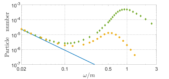
Figure 1: Plot of the mean number of created particles as a function of $\omega$ for the profile (19) with $E=E_{S}/3$. The yellow circles denote the results of the Dirac-Heisenberg-Wigner formalism, the green diamonds correspond to the spatially homogeneous field approximation and the blue line displays the locally constant field approximation.

The computed mean particle numbers are plotted in Fig. 1. The locally constant field approximation just reflects the trivial space-time volume scaling with $1/\omega^{2}$. As expected, the results of the Dirac-Heisenberg-Wigner formalism converge to that approximation for small $\omega$, i.e., small Keldysh parameters (3), but start to show significant deviations for Keldysh parameters of order unity, which is the regime we are interested in.

Motivated by the above findings based on the WKB approach, we also compared those results with the spatially homogeneous field approximation: To this end, we calculated the pair-creation probability $P$ for a purely time-dependent scenario $\mbox{\boldmath$A$}(t)=2f(ct)\mbox{\boldmath$e$}_{y}$ corresponding to the field at the symmetry plane $x=0$ Hebenstreit ; Kluger ; Schmidt . While this is expected to yield the correct pair-creation exponent, this scenario grossly overestimates the pre-factor because particles are now created in the whole spatial volume. For the colliding pulses (2), however, pair creation predominantly occurs in the vicinity of the symmetry plane $x=0$ where the electric field assumes its maximum. In order to correct this over-estimation, we introduce a pre-factor accounting for the finite extent (in $x$-direction) of the effective pair-creation volume footnote2 . As a natural and minimal assumption, we take this pre-factor to be proportional to $1/\omega$, i.e., the pulse width, where the proportionality constant is fixed by demanding convergence to the locally constant field approximation at small $\omega$, see also PhysRevD.93.025014 ; PhysRevD.91.045016 ; STROBEL20141153 ; PhysRevD.99.016020 ; PhysRevD.78.061701 .

As we may observe in Fig. 1, this spatially homogeneous field approximation still over-estimates the pair-creation probability a bit, but provides a much better description than the locally constant field approximation. Even for frequencies of the order of the electron mass, it reproduces the qualitative behavior of the full Dirac-Heisenberg-Wigner results, such as the peak of the particle number at $\omega=\,{\cal O}(m)$. The quantitative disagreement regarding the height and location of the peaks can presumably be explained by a threshold effect marking the transition from the non-perturbative to the perturbative regime at large $\omega$ (where the WKB approach is expected to break down), see Section E in the Supplemental Material Supplement .

Focusing/de-focusing corrections

The spatially homogeneous field approximation explained above does only take into account the $\ddot{s}$ term in Eqs. (Particle creation), i.e., the electric field $E_{y}$. In order to include the effects of the magnetic field $B_{z}$, one should replace $\ddot{s}\to\Box s$, cf. Eqs. (Particle creation), which also contains $\partial_{x}^{2}s$, i.e., the curvature $s_{2}$ in Eq. (10). The effect of this replacement can be studied by numerically solving the set of ordinary differential equations (8), (10) and (Particle creation) for the profile (19). As example parameters, we choose $E=E_{S}/3$ as before and $\omega=m/3$, i.e., $\gamma=1$.

As shown in Section C of the Supplemental Material Supplement , the behavior of $\ddot{s}_{0}(t)$ and $s_{2}(t)$ strongly depends on the momentum $k_{y}$. For $k_{y}=\pm m$, for example, the curvature $s_{2}(t)$ is quite close to $\ddot{s}_{0}(t)$ thus almost canceling each other in the pre-factor $\Box s$. For $k_{y}=0$, this is not the case as the curvature $s_{2}(t)$ varies more slowly with time than $\ddot{s}_{0}(t)$.

We find that including the curvature term $s_{2}$ reduces the pair-creation probability, e.g., roughly by a factor of two for the case $k_{y}=0$ (which yields the dominant contribution), see the Supplemental Material Supplement . Thus, including the focusing/de-focusing effects corrects the over-estimate of the spatially homogeneous field approximation and brings the estimated pair-creation probability almost on top of the value obtained by the Dirac-Heisenberg-Wigner approach. However, more systematic investigations are needed to assess the overall accuracy of this approach.

Conclusions

As a prototypical example for a space-time dependent and transversal field configuration (as a vacuum solution to the Maxwell equations), we consider the head-on collision of two plane-wave laser pulses. Via the WKB approach, we study electron-positron pair creation in this background for sub-critical fields $E\ll E_{S}$ and Keldysh parameters of order unity. Along the symmetry (i.e., collision) plane, where we expect that dominant contribution, we find that the pair-creation exponent is the same as for a purely time-dependent electric field, only the pre-factor $\ddot{s}\to\Box s$ does also include the impact of the magnetic field, leading to focusing/de-focusing effects.

This approximate mapping to a purely time-dependent electric field allows us to employ the spatially homogeneous field approximation, which we compare to numerical simulations using the Dirac-Heisenberg-Wigner approach. We find that the spatially homogeneous field approximation over-estimates the pair-creation probability slightly, but provides a much better description than the locally constant field approximation, see Fig. 1. It even reproduces qualitative features of the pair-creation spectra, see Section D in the Supplemental Material Supplement .

Going beyond the spatially homogeneous field approximation, we may also study the impact of the magnetic field, leading to focusing/de-focusing effects. Along the symmetry plane, this amounts to replacing $\ddot{s}$ by $\Box s$ in the evolution equations for the Bogoliubov coefficients, which also contains the curvature term $\partial_{x}^{2}s$. For the cases we studied, we found that this replacement tends to lower the pair-creation probability, which brings it closer to the results of the Dirac-Heisenberg-Wigner approach.

However, one might also imagine other scenarios. Note that $\ddot{s}$ is a local function of $A_{y}$ and $\dot{A}_{y}$, while the curvature $\partial_{x}^{2}s$ is non-local, i.e., depends on whole history of the evolution. This could be exploited in pulse-shape optimization schemes aimed at increasing the pair-creation probability. As an intuitive picture, if the initial wave-packet of the fermionic quantum vacuum fluctuations is focused onto the symmetry plane, where the electric field assumes its maximum, it can react to this strong field (i.e., produce particles) much better than a wave-packet which is more de-localized.

Experimental scenarios

Finally, let us discuss potential experimental tests of our results. Ultra-strong optical laser foci have very small Keldysh parameters $\gamma\ll 1$ and should thus be treatable via the locally constant field approximation. X-ray free electron lasers (XFEL), on the other hand, have much larger $\gamma$ and could require going beyond that approximation. Unfortunately, however, present-day facilities do not reach the necessary field strengths $E$ yet. An interesting idea to achieve this goal is high-harmonic focusing (see, e.g., PhysRevLett.94.103903 ; PhysRevLett.123.105001 ; PhysRevLett.127.114801 ) which typically also corresponds to non-negligible $\gamma$.

As a completely different scenario for generating ultra-strong fields, collisions of heavy nuclei have been studied theoretically and experimentally, see, e.g., PhysRevLett.127.052302 ; Reinhardt ; Schweppe ; Cowan ; Ahmad ; Maltsev . Considering ultra-peripheral “collisions” at relativistic velocities $v$ along the trajectories $\mbox{\boldmath$r$}(t)=\pm(vt,b/2,0)^{T}$ with impact parameters $b$, the superpositions of the boosted Coulomb fields of the two nuclei can be approximated by Eq. (2) at sufficiently large distances $|\mbox{\boldmath$r$}|\gg b$, say, of the order of the Compton length electron-bunch ; magnetic-monopole . The associated field strengths may reach or even exceed the Schwinger critical field $E_{S}$ HeavyIon ; ATLAS and the Keldysh parameters $\gamma$ will also be non-negligible (especially for ultra-relativistic $v$). Of course, the field strengths and their spatial and temporal gradients will be even larger at smaller distances $|\mbox{\boldmath$r$}|\sim b$, such that the total electron-positron yield will also contain contributions from this region. Nevertheless, this again shows the importance of understanding the impact of space-time dependence on pair creation, i.e., to go beyond the locally constant field approximation.

Appendix A A. World-line instanton technique

It might be illuminating to study the colliding-pulse scenario in Eq. (2) via the world-line instanton technique. This method is another semi-classical approach and allows us to estimate the pair-creation probability $P$ via Affleck ; PhysRevD.72.105004

$$P\sim\exp\left\{-{\cal A}_{\rm inst}\right\}\,,$$ (S1)

where ${\cal A}_{\rm inst}$ is the action of the associated world-line instanton, i.e., a closed loop $x^{\mu}(\tau)$ in Euclidean space-time as a solution of the Euclidean semi-classical or classical equations of motion

$$m\frac{d^{2}x^{\mu}}{d\tau^{2}}=qF^{\mu\nu}\frac{dx_{\nu}}{d\tau}\,,$$ (S2)

parametrized by the “proper” time $\tau$.

As explained after Eq. (2), the magnetic field vanishes in the $x=0$ plane and thus the Euclidean field strength tensor $F^{\mu\nu}(x=0)$ does only contain the electric field $E_{y}$. As a result, the instanton moves in imaginary time and $y$-direction, but stays on the $x=0$ plane, which yields the same exponent ${\cal A}_{\rm inst}$ as for a purely time-dependent field $\mbox{\boldmath$A$}(t)=2f(ct)\mbox{\boldmath$e$}_{y}$, see also Linder ; PhysRevD.84.125023 .

Within the world-line instanton technique, the pre-factor in front of the exponential (S1) can be obtained (at least in principle) by considering perturbations around the instanton trajectory, but such a calculation can be quite non-trivial for genuinely space-time-dependent fields PhysRevD.73.065028 ; footnote-prefactor .

Appendix B B. Dirac-Heisenberg-Wigner approach

Let us provide a brief outline of the Dirac-Heisenberg-Wigner approach Vasak:1987umA . We start from the Lagrangian

$${\mathcal{L}}=\frac{1}{2}\left({\rm i}\bar{\Psi}\gamma^{\mu}\mathcal{D}_{\mu}\Psi-{\rm i}\bar{\Psi}\mathcal{D}_{\mu}^{{\dagger}}\gamma^{\mu}\Psi\right)-m\bar{\Psi}\Psi$$ (S3)

with the Dirac matrices $\gamma^{\mu}$ and the covariant derivatives $\mathcal{D}_{\mu}=\partial_{\mu}+{\rm i}qA_{\mu}$ and $\mathcal{D}_{\mu}^{{\dagger}}=\overset{\leftharpoonup}{\partial_{\mu}}-{\rm i}qA_{\mu}$. As usual in the Furry picture, the Dirac spinors $\bar{\Psi}$ and ${\Psi}$ are treated as dynamical quantum fields whereas the electromagnetic vector potential $A_{\mu}$ is an external field, i.e., a c-number. As is well known, by doing so we neglect higher-order interactions, e.g., radiative emission, backreaction or electron-electron coupling Fauth ; PhysRevD.87.105006 ; Bloch ; PhysRevD.87.125035 ; PhysRevSTAB.14.054401 ; PhysRevLett.105.080402 .

Considering bilinear forms of the Dirac spinors $\hat{\bar{\Psi}}$ and ${\hat{\Psi}}$ at different space-time points $x_{1}^{\mu}$ and $x_{2}^{\mu}$, we may transform them to center-of-mass ${\mathfrak{r}}^{\mu}=(x_{1}^{\mu}+x_{2}^{\mu})/2$ and relative coordinates ${\mathfrak{s}}^{\mu}=x_{1}^{\mu}-x_{2}^{\mu}$ which yields the generalized density operator

$$\hat{\mathcal{C}}_{\alpha\beta}\left({\mathfrak{r}},{\mathfrak{s}}\right)=\mathcal{U}_{A}\left({\mathfrak{r}},{\mathfrak{s}}\right)\left[\hat{\bar{\Psi}}_{\beta}\left({\mathfrak{r}}-{\mathfrak{s}}/2\right),\hat{\Psi}_{\alpha}\left({\mathfrak{r}}+{\mathfrak{s}}/2\right)\right],$$ (S4)

where the Wilson line factor

$$\mathcal{U}_{A}\left({\mathfrak{r}},{\mathfrak{s}}\right)=\exp\left(\mathrm{i}q\int_{-1/2}^{1/2}{\rm d}\xi\ {\mathfrak{s}}^{\mu}A_{\mu}\left({\mathfrak{r}}+\xi{\mathfrak{s}}\right)\right)$$ (S5)

is implemented to ensure gauge-invariance.

The Fourier transform of this quantity (S4) with respect to the relative coordinate ${\mathfrak{s}}^{\mu}=x_{1}^{\mu}-x_{2}^{\mu}$ yields the covariant Wigner operator Vasak:1987umA in $2+1$ dimensions

$$\hat{\mathcal{W}}_{\alpha\beta}\left({\mathfrak{r}},p\right)=\frac{1}{2}\int{\rm d}^{3}{\mathfrak{s}}\ \mathrm{e}^{\mathrm{i}p_{\mu}{\mathfrak{s}}^{\mu}}\ \hat{\mathcal{C}}_{\alpha\beta}\left({\mathfrak{r}},{\mathfrak{s}}\right),$$ (S6)

where $p_{\mu}$ can be identified as the kinetic or mechanical momentum because the vector potential $A_{\mu}$ is already contained in the Wilson line factor (S5). Thus $\hat{\mathcal{W}}_{\alpha\beta}$ represents a kinetic quantity defined in the particles’ coordinate-momentum phase-space.

The time evolution of the Wigner operator is determined by the Dirac equation. In order to formulate transport equations, we take its expectation value in the initial vacuum state $|0\rangle$ which yields the Wigner function

$$\mathbbm{W}\left({\mathfrak{r}},p\right)=\langle 0|\hat{\mathcal{W}}\left({\mathfrak{r}},p\right)|0\rangle,$$ (S7)

where we omitted the indices for the sake of simplicity.

We expand the Wigner function in Dirac bilinears in an irreducible representation

$$\mathbbm{W}\left({\mathfrak{r}},p\right)=\frac{1}{2}\left(\mathbbm{1}\mathbbm{S}+\gamma^{\mu}\mathbbm{V}_{\mu}\right),$$ (S8)

where the gamma matrices are (in 2+1 dimensions) given in terms of the Pauli matrices

$$\gamma^{0}=\sigma_{3},\ \gamma^{1}=i\sigma_{1},\ \gamma^{2}=-i\sigma_{2}.$$ (S9)

Transport equations

Projection on equal-time

$$\mathbbm{w}(t,\boldsymbol{x},\boldsymbol{p})=\int\frac{{\rm d}p_{0}}{2\pi}\,\mathbbm{W}({\mathfrak{r}},p),$$ (S10)

with ${\mathfrak{r}}=(t,\boldsymbol{x})$ gives rise to a closed set of differential equations describing the time evolution of particle distributions, namely mass $\mathbbm{s}$, charge $\mathbbm{v}_{\mathbb{0}}$ and current $\boldsymbol{\mathbbm{v}}$ density Vasak:1987umA ; BB ; Ochs . For a potential of the form (2), within QED₂₊₁ and one set of $2$-spinors we obtain on the basis of $p_{x}=k_{x},~{}p_{y}=k_{y}+q\int{\rm d}\xi\ A_{y}\left(x+\xi{\mathfrak{s}}_{x},t\right)$ Kohlf ; PhysRevD.101.096009 ; KOHLFURST2016371

$$\partial_{t}\ \mathbbm{s} +2k_{x}\ \mathbbm{v}_{2} -2\Pi\ \mathbbm{v}_{1} =0,$$ (S11)

$$\partial_{t}\ \mathbbm{v}_{\mathbb{0}} +D\ \mathbbm{v}_{2} +\partial_{x}\ \mathbbm{v}_{1} =0,$$ (S12)

$$\partial_{t}\ \mathbbm{v}_{1} +\partial_{x}\ \mathbbm{v}_{0} +2\Pi\ \mathbbm{s} =+2m\ \mathbbm{v}_{2},$$ (S13)

$$\partial_{t}\ \mathbbm{v}_{2} +D\ \mathbbm{v}_{0} -2k_{x}\ \mathbbm{s} =-2m\ \mathbbm{v}_{1},$$ (S14)

with pseudo-differential operators KohlfurstNew

$$D = +{\rm i}q\ \mathcal{F}^{-1}_{k_{x}}\ \left[A_{y}\left(x+\frac{{\mathfrak{s}}_{x}}{2},t\right)-A_{y}\left(x-\frac{{\mathfrak{s}}_{x}}{2},t\right)\right]\mathcal{F}_{k_{x}},$$ (S15)

$$\Pi =k_{y} +\frac{q}{2}\ \mathcal{F}^{-1}_{k_{x}}\ \left[A_{y}\left(x+\frac{{\mathfrak{s}}_{x}}{2},t\right)+A_{y}\left(x-\frac{{\mathfrak{s}}_{x}}{2},t\right)\right]\mathcal{F}_{k_{x}}.$$ (S16)

Here, the Fourier operators $\mathcal{F}_{k_{x}}$ transform from canonical momentum space $k_{x}$ to relative coordinate space ${\mathfrak{s}}_{x}$. As a matter of fact, Eqs. (S11)-(S14) describe a partial differential equation in $t,x$ and $k_{x}$ with the (conserved) canonical momentum $k_{y}$ serving as an external parameter.

In order to determine the pair production rate from an initial vacuum state, we employ initial conditions of the form

$$\mathbbm{s}_{\rm vac}\left(\boldsymbol{k}\right)=-\frac{m}{\sqrt{m^{2}+\boldsymbol{k}^{2}}},\qquad \boldsymbol{\mathbbm{v}}_{\rm vac}\left(\boldsymbol{k}\right)=-\frac{\boldsymbol{k}}{\sqrt{m^{2}+\boldsymbol{k}^{2}}},\qquad \mathbbm{v}_{\mathbb{0}}{}_{\rm vac}=0.$$ (S17)

Evaluating the transport equations on the basis of these initial conditions, we obtain the particle distribution function at asymptotic times ($t\to\pm\infty$)

$$n\left(\boldsymbol{x},\boldsymbol{k}\right)=\frac{m\left(\mathbbm{s}-\mathbbm{s}_{\rm vac}\right)+\boldsymbol{k}\cdot\left(\boldsymbol{\mathbbm{v}}-\boldsymbol{\mathbbm{v}}_{\rm vac}\right)}{2\sqrt{m^{2}+\boldsymbol{k}^{2}}}.$$ (S18)

The total particle number is given by

$$N=\int\ \frac{{\rm d}^{2}k\ {\rm d}^{2}x}{(2\pi)^{2}}\ n\left(\boldsymbol{x},\boldsymbol{k}\right).$$ (S19)

Spatially homogeneous approximation

In the spatially homogeneous field approximation we calculate a fully time-dependent, but spatially localized pair production rate ($x=0$) on the basis of Eqs. (S11)-(S14), see also footnote2 .

At $x=0$ the vector potential takes on the form $\mbox{\boldmath$A$}(t)=2f(ct)\mbox{\boldmath$e$}_{y}$, see Eq. (19). Consequently, the differential operators (S15)-(S16) simplify to ordinary factors, $D=0$ and $\Pi=qA_{y}$. Furthermore, within an entirely localized description of particle creation, particle propagation can be neglected thus derivatives with respect to spatial coordinates vanish.

As a result, the corresponding equations of motion take on the much simpler form

$$\partial_{t}\ {\mathbbm{s}}^{\rm SHA} +2k_{x}\ {\mathbbm{v}}_{2}^{\rm SHA} -2\left(k_{y}+qA_{y}(t)\right)\ {\mathbbm{v}}_{1}^{\rm SHA} =0,$$ (S20)

$$\partial_{t}\ {\mathbbm{v}}_{1}^{\rm SHA} +2\left(k_{y}+qA_{y}(t)\right)\ {\mathbbm{s}}^{\rm SHA} =+2m\ {\mathbbm{v}}_{2}^{\rm SHA},$$ (S21)

$$\partial_{t}\ {\mathbbm{v}}_{2}^{\rm SHA} -2k_{x}\ {\mathbbm{s}}^{\rm SHA} =-2m\ {\mathbbm{v}}_{1}^{\rm SHA},$$ (S22)

where we used the superscript ${\rm SHA}$ (spatially homogeneous approximation) to indicate that these components do not depend on $x$. Initial conditions remain unchanged, see Eq (S17). Equations (S20)-(S22) can also be derived employing a quantum kinetic approach Hebenstreit ; Kluger ; Schmidt .

Locally constant field approximation

Within the locally constant field approximation we assume instantaneous particle creation. While this approximation fails to capture time-memory effects, e.g., photon absorptive processes, it is expected to provide correct particle numbers if spatial and temporal variations in the employed fields are sufficiently smooth.

For a field of the form $\mbox{\boldmath$A$}(t,\mbox{\boldmath$r$})$ we model the source term heuristically after the Sauter-Schwinger effect in constant fields Nikishov2 in $2+1$ dimensions Lin

$${\mathcal{S}}=\frac{\lvert q\rvert^{3/2}\ a(t,x)^{3/2}}{(2\pi)^{2}}\exp\left(-\frac{\pi m^{2}}{\lvert q\rvert a(t,x)}\right),$$ (S23)

with $a(t,x)=\sqrt{\lvert{\mathcal{F}(t,x)}\rvert-{\mathcal{F}(t,x)}}$ and ${\mathcal{F}}(t,x)=-1/2\ \big{(}E(t,x)^{2}-B(t,x)^{2}\big{)}$. In order to obtain the total particle number integrations over all coordinates are in order, $N_{\rm LCFA}=\int{\rm d}t\ \int{\rm d}x\ {\mathcal{S}}(t,x)$.

Appendix C C. Curvature contribution

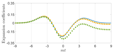
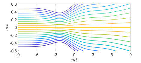
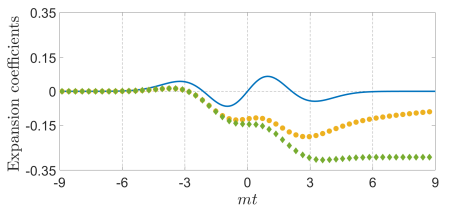
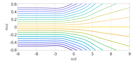
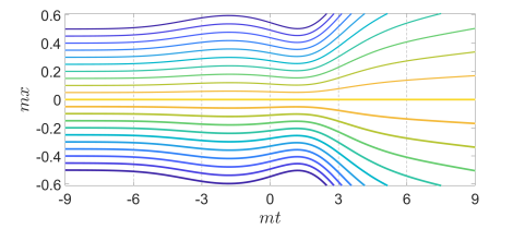
Figure S1: Left panel: Time evolution of $\ddot{s}_{0}$ (blue line) in Eq. (8) and the curvature $s_{2}$ in Eq. (10) in the linear (green diamonds) and non-linear (orange circles) form, respectively. Data are obtained for the profile (19) with $E=E_{S}/3$, $\omega=m/3$ and $k_{y}=-m$ (top), $k_{y}=0$ (middle), $k_{y}=m$ (bottom). In the right panel, we display a set of characteristic curves Oertel for the same parameters in order to visualize the focussing/de-focussing effects – where one may observe a strong correlation to the behavior of $s_{2}$, as expected from the discussion after Eq. (10).

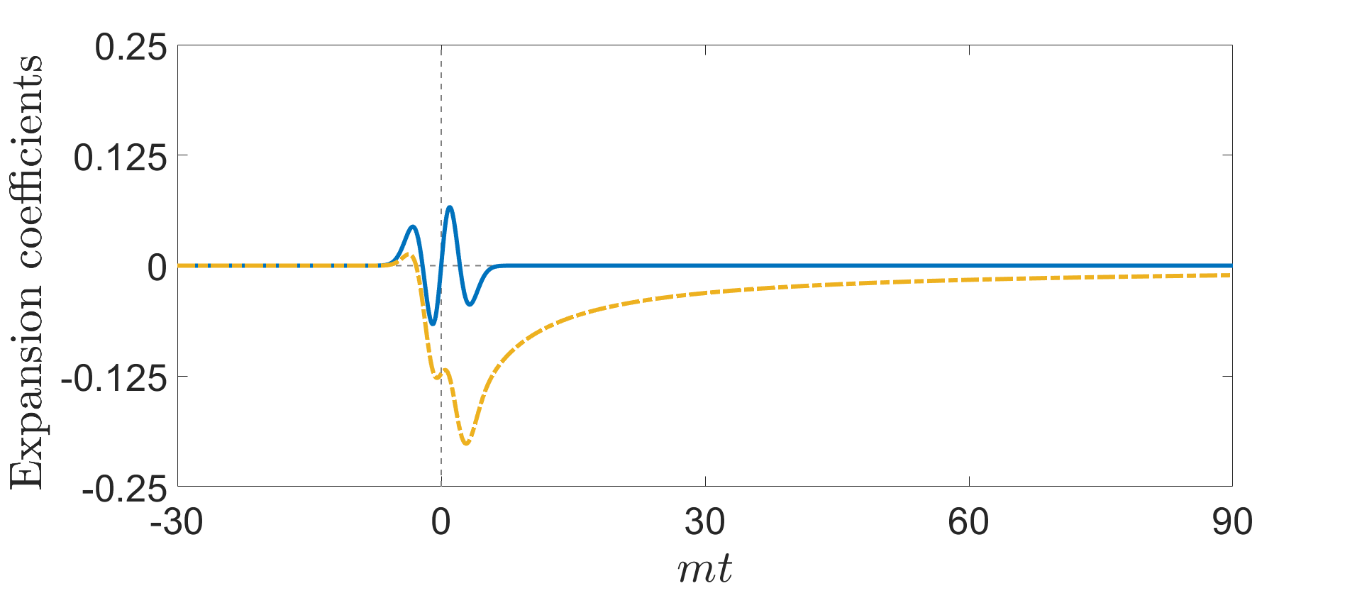
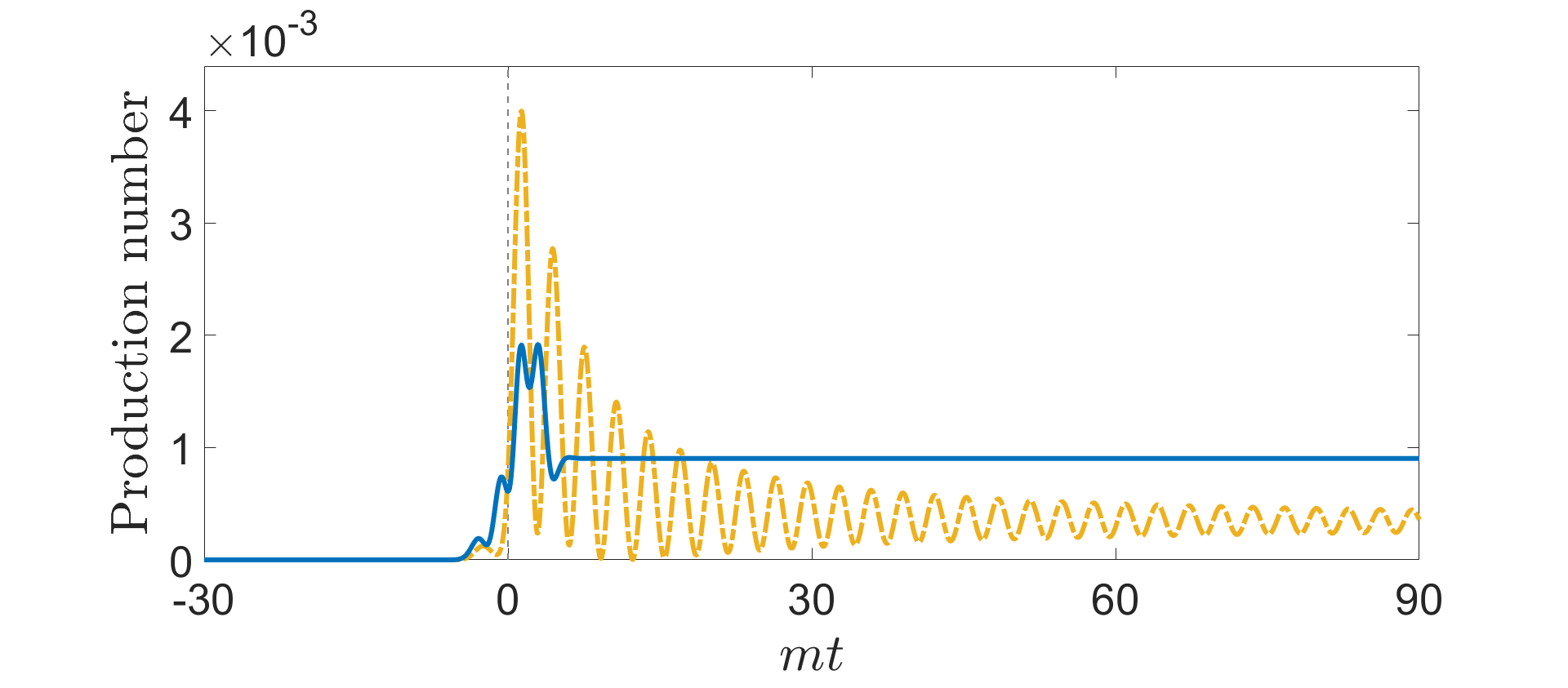
Figure S2: Time evolution of $\ddot{s}_{0}$ (solid blue line) in Eq. (8) and the curvature $s_{2}$ (dashed orange line) in Eq. (10) as in Fig. S1 (top); the quantity $\lvert R\rvert^{2}$ associated with the rate of particle creation, obtained in the spatially homogeneous field approximation (solid blue line), i.e., just from $\ddot{s}_{0}$, in comparison to the full solution (dashed orange line) obtained by replacing $\ddot{s}_{0}\to\Box s=\ddot{s}_{0}-s_{2}$ taking into account the focusing/de-focusing corrections (bottom). Data are obtained for the profile (19) with $E=E_{S}/3$, $\omega=m/3$ and $k_{y}=0$.

Solving Eq. (10) numerically, we plot the evolution of the curvature $s_{2}$ (starting at zero) in comparison to $\ddot{s}_{0}$ for $E=E_{S}/3$, $\omega=m/3$ and the values $k_{y}=0$ and $k_{y}=\pm m$ in Fig. S1.

As our first observation, we find no blow-up singularities for these parameters. Furthermore, we compare the full solution of the non-linear differential equation (10) with its linearized approximation obtained by neglecting the nonlinearity $s_{2}^{2}$ in Eq. (10). We find reasonably good agreement in the time interval relevant for pair creation. Note that the potential blow-up singularities are caused by the nonlinearity $s_{2}^{2}$ in Eq. (10) and thus never occur in the linearized solution.

For $k_{y}=\pm m$, we see that the curvature $s_{2}(t)$ lies very close to $\ddot{s}_{0}(t)$. As a result, this curvature contribution (stemming from the magnetic field) almost completely cancels the term $\ddot{s}_{0}(t)$ in the pre-factor $\Box s$ of the evolution equations (Particle creation) for the Bogoliubov coefficients, leading to a significantly reduced pair creation. This cancellation does not occur for $k_{y}=0$, but the pair creation probability is still reduced by roughly a factor of two, see Fig. S2 and Section G below.

Whether the differences between the full Dirac-Heisenberg-Wigner data and the results of the spatially homogeneous field approximation observed in Fig. S3 below, most notably the “shoulders” of the curve with $\omega=m/3$ starting around $|k_{y}|\approx m/2$, can be traced back (at least partially) to this cancellation for large $|k_{y}|$ should be investigated in future studies.

For the sake of completeness, we also examine the characteristic curves for a better visualization of focusing and de-focusing effects created by the inhomogeneity in the field. To this end, we employ the method of characteristics in order to turn Eq. (6) into a family of first-order, ordinary differential equations

$$\dot{x}_{0}(\tau)=\frac{2}{m}p_{0}(\tau),\,\dot{x}_{1}(\tau)=-\frac{2}{m}p_{1}(\tau),\,\dot{p}_{0}(\tau)=\frac{2}{m}\left(k_{y}+qA_{y}\right)\left(qE_{y}\right),\,\dot{p}_{1}(\tau)=\frac{2}{m}\left(k_{y}+qA_{y}\right)\left(qB_{z}\right),$$ (S24)

with $p_{0}=\partial_{t}s$ and $p_{1}=\partial_{x}s$, respectively. The parameter $\tau$ specifies the location on a distinctive characteristic curve determined by a particular initial condition. A set of solutions obtained by varying the initial starting position $x_{1,{\rm init}}$ is displayed in Fig. S1. It is apparent that there is a strong correlation between $s_{2}$ being positive/negative and the curves coming closer or being dispersed, respectively.

Appendix D D. Particle spectra

While the world-line instanton technique – at least in its simplest form discussed above – only yields the total pair creation probability (S1), the WKB and Dirac-Heisenberg-Wigner approaches allow direct access to the particle spectra. Since $k_{x}$ is not a conserved quantity in our case (2), we focus on the $k_{y}$-dependence. Figure S3 displays exemplary spectra for the frequency values $\omega=m/3$, $\omega=m/4$ and $\omega=m/5$, where we have used the same scenario as in Fig. 1, i.e., the profile (19) with $E=E_{S}/3$. Shown are the results of the Dirac-Heisenberg-Wigner approach in comparison to the spatially homogeneous field approximation (after re-scaling), which are basically the spectra produced by a purely time-dependent field.

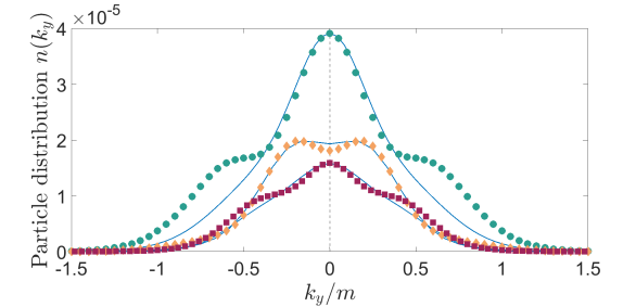
Figure S3: Plot of the pair-creation spectra obtained by the spatially homogeneous field approximation for the profile (19) with $E=E_{S}/3$ and $\omega=m/3$ (green circles), $\omega=m/4$ (orange diamonds), and $\omega=m/5$ (red squares). The data have been rescaled by a constant factor in order to compensate the overestimation mentioned above. For comparison, the blue curves correspond to the results obtained through the Dirac-Heisenberg-Wigner approach.

We find that the spectra obtained by the two approaches match quite well, especially for small $k_{y}$ (consistent with the considerations in the previous Section), but there are also distinctive differences. Most notably, the spatially homogeneous field approximation predicts two “shoulders” starting around $k_{y}\approx\pm m/2$ in the spectrum for $\omega=m/3$, which are not reproduced by the Dirac-Heisenberg-Wigner approach. These differences might be explainable by the additional curvature contributions $s_{2}$ discussed in the previous Section, but further investigations are necessary to settle this point.

As another interesting feature, both approaches agree on a plateau or even dip at small $k_{y}$ in the spectrum for $\omega=m/4$. This is quite remarkable since it seems to contradict the standard expectation that the spectrum should have its maximum at $k_{y}=0$. Assuming that the particles are predominantly created at $t=0$ (i.e., the maximum of the electric field) and with vanishing initial velocity $v_{y}(t=0)=0$, one would indeed expect the spectrum to have its maximum at $k_{y}=0$ in view of $A_{y}(t=0)=A_{y}(t\to\pm\infty)=0$. Investigating the reasons for this apparent contribution (e.g., interference phenomena, see also PhysRevLett.108.030401 ; PhysRevD.98.056009 ; PhysRevD.83.065028 ) should be the subject of further studies.

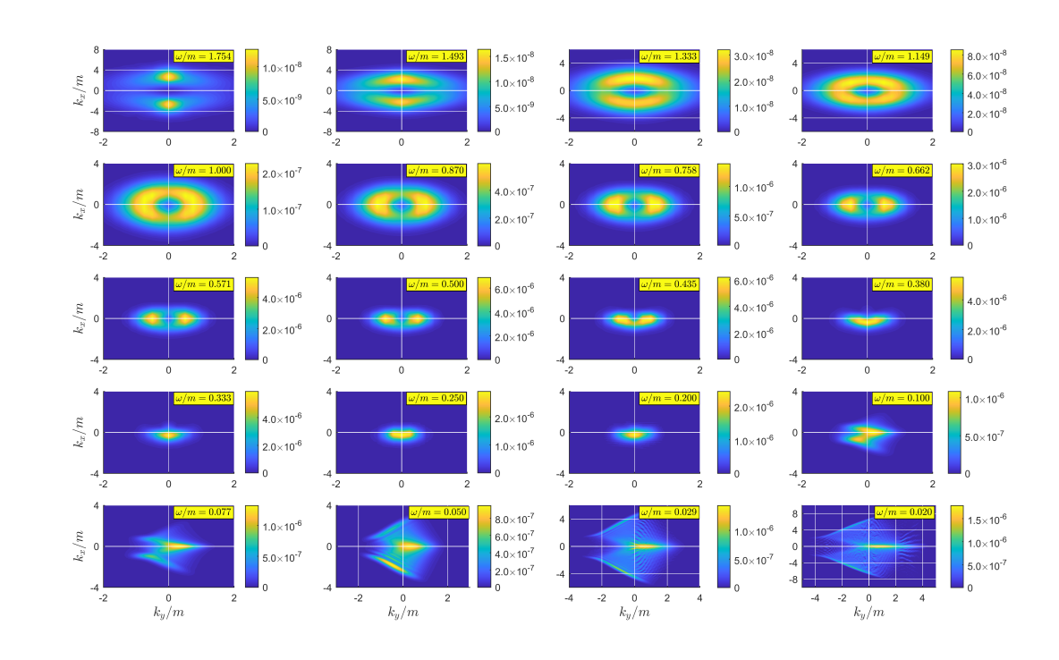
Figure S5: Particle momentum spectra obtained from solving the Dirac-Heisenberg-Wigner transport equations for a field profile of two identical, colliding laser pulses (2). The field strength is given by $E=E_{S}/3$, the different pulse frequencies are displayed as insets. Through integration over the momentum space variables $k_{x}$ and $k_{y}$ the mean number of created particles is obtained, cf. the orange circles in Fig. 1.

For the sake of completeness, we illustrate the two-dimensional spectra (displaying the dependence on $k_{x}$ and $k_{y}$) obtained through solving the transport equations (S11)-(S14) for a variety of parameters in Fig. S5. Note that integrating these spectra over $k_{x}$ yields the blue curves in Fig. S3 while another integration over $k_{y}$ then gives the total particle number, i.e., the orange curve in Fig. 1.

Appendix E E. Threshold effects

As a working hypothesis, we interpret the peaks observed in Fig. 1 as threshold effects marking the transition from the non-perturbative to the perturbative regime. In order to test this hypothesis, we study the dependence of these peaks on the maximum electric field strength $E$ in Fig. S4.

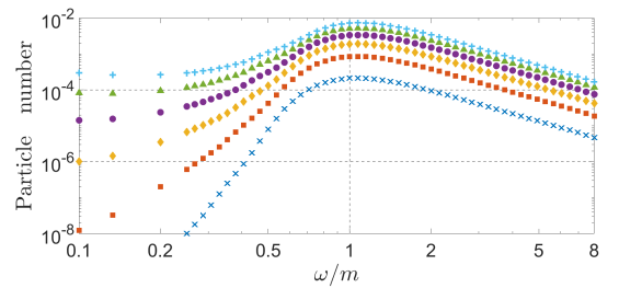
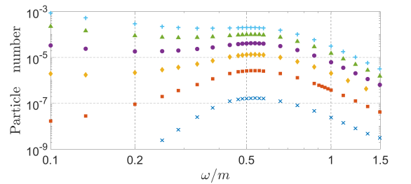
Figure S4: Mean number of created particles as a function of $\omega$ for various field strengths $E/E_{S}\in\{0.1,0.2,\ldots,0.6\}$, for a purely time-dependent profile (19) at the left and the collision scenario (2) at the right.

To lowest (non-vanishing) order perturbation theory, one would expect an $E^{4}$-scaling of the mean particle number in the collision scenario (2) where two photons collide to form an electron-positron pair. Such an $E^{4}$-scaling is indeed consistent with the dependence of the peak heights as well as the behavior of the curves for larger frequencies in Fig. S4 (right). For smaller frequencies, however, the curves display deviations from this scaling, indicating the failure of lowest-order perturbation theory.

For purely time-dependent fields, one would expect an $E^{2}$-scaling instead, as already the first-order amplitude in $E$ can account for pair creation. Again, this scaling is consistent with the peak heights as well as the behavior for larger frequencies in Fig. S4 (left), while the dependence at smaller frequencies deviates.

These perturbative arguments can also help to understand the different locations of the peaks. While the collision of two photons with frequency $\Omega\geq m$ may create $e^{+}e^{-}$-pairs in the collision scenario, a purely time-dependent field must contain frequency components with $\Omega\geq 2m$ in order to obtain a non-zero first-order amplitude in $E$. Consistently, the peak of the collision scenario occurs at lower frequencies than that for purely time-dependent fields.

Note that making these points more precise is complicated by the fact that the Fourier transform of the field profile (19) yields a rather broad frequency spectrum which has its maximum at a frequency of $\Omega=2\omega$. Elucidating this issue should be the subject of further studies.

Appendix F F. Blow-up singularities

Let us study the presence or absence of blow-up singularities in the curvature contribution $s_{2}(t)$ in more detail. First, we focus on the case $k_{y}=k_{z}=0$ for simplicity and consider large Keldysh parameters $\gamma\gg 1$, i.e., $qE\ll m\omega$. In this limit, we have $qA_{y}\ll m$ and using $\partial_{x}^{2}A_{y}=\partial_{t}^{2}A_{y}=\,{\cal O}(\omega E)$, we find that $s_{2}$ scales with $s_{2}=\,{\cal O}(qE/\gamma)$, i.e., $s_{2}\ll qE$. Altogether, we may simplify Eq. (10) via

$$\dot{s}_{2}=\left.\frac{s_{2}^{2}+\left[k_{y}+qA_{y}\right]q\partial_{x}^{2}A_{y}}{\sqrt{m^{2}+\left[k_{y}+qA_{y}\right]^{2}+k_{z}^{2}}}\right\rvert_{x=0}\approx\left.\frac{q^{2}A_{y}\ddot{A}_{y}}{m}\right\rvert_{x=0}=-\left.\frac{q^{2}(\dot{A}_{y})^{2}}{m}\right\rvert_{x=0}+\left.\frac{d}{dt}\left(\frac{q^{2}A_{y}\dot{A}_{y}}{m}\right)\right\rvert_{x=0}\,.$$ (S25)

Apart from the total derivative in the last term, we find that $\dot{s}_{2}$ is negative. Thus, $s_{2}(t)$ may oscillate during the collision of the two pulses, but assumes a negative value afterwards. The subsequent evolution is then governed by the non-linearity $\dot{s}_{2}=s_{2}^{2}/m$ which implies that $s_{2}(t)$ is slowly approaching the $t$-axis from below as $1/t$. Blow-up singularities would occur if $s_{2}$ was positive after the collision and could be visualized as self-focusing, but they are absent in this case and the de-focusing effects dominate.

Actually, as we have observed in Fig. S1, the linearization (i.e., neglect of $s_{2}^{2}$) provides a fairly good approximation even for moderate values of $k_{y}=\,{\cal O}(m)$ and for Keldysh parameters $\gamma$ of order unity. Thus, if we rewrite $\dot{s}_{2}$ as

$$\dot{s}_{2}=-\left.\frac{q^{2}\dot{A}_{y}^{2}m^{2}}{\left(m^{2}+\left[k_{y}+qA_{y}\right]^{2}+k_{z}^{2}\right)^{3/2}}\right\rvert_{x=0}+\left.\frac{d}{dt}\left(\frac{q\dot{A}_{y}\left[k_{y}+qA_{y}\right]}{\sqrt{m^{2}+\left[k_{y}+qA_{y}\right]^{2}+k_{z}^{2}}}\right)\right\rvert_{x=0}+\,{\cal O}(s_{2}^{2})\,,$$ (S26)

we again find a negative value of $s_{2}$ after the collision, provided that the non-linearity $s_{2}^{2}$ can be neglected during the collision. Thus, for moderate values of $\gamma$ and $k_{y}$ (note that $k_{z}$ can simply be absorbed into $m$), we basically get the same picture as above, i.e., an approximately linear evolution of $s_{2}(t)$ during the collision resulting in a negative value of $s_{2}$ after the collision, which then implies a slow $1/t$-decay of $|s_{2}|$ governed by the non-linear evolution.

Consistent with these analytic approximations, we only found blow-up singularities in our numerical simulation for very large $k_{y}$ and/or for extremely long pulses (which can be treated via the locally constant field approximation).

Appendix G G. Bogoliubov coefficients

The Bogoliubov coefficients $\alpha(t,x=0)$ and $\beta(t,x=0)$ along the symmetry plane can either be obtained by solving Eqs. (15) directly or from the Riccati equation $\dot{R}=\Box s(e^{+2is}-R^{2}e^{-2is})/(2\chi)$ together with their normalization. For our choice of the eigenvectors $\mbox{\boldmath$u$}_{\pm}=(1,\pm i\chi)^{T}$, the normalization of the Bogoliubov coefficients along the symmetry plane can be derived from Eqs. (15) and reads

$$\left|\alpha(t,x=0)\right|^{2}-\left|\beta(t,x=0)\right|^{2}=\exp\left\{-\frac{1}{2}\int\limits_{-\infty}^{t}dt^{\prime}\,\left.\frac{\Box s}{\chi}\right\rvert_{t^{\prime},x=0}\right\}\,.$$ (S27)

For purely time-dependent fields $\Box s=\ddot{s}$, the integrand $\ddot{s}/\chi=\ddot{s}/\dot{s}$ in Eq. (S27) is a total derivative and thus we recover the well-known $1/\sqrt{\chi}$ normalization. Including the spatial curvature $s_{2}$ also incorporates focusing/de-focusing effects. Actually, inserting the dependence $s_{2}(t)\propto 1/t$ for late times (as explained above), the right-hand side of Eq. (S27) behaves as $1/\sqrt{t}$ which corresponds to the spread of the wave packets. Obviously, this does not imply that the number of created particles decreases – their number should be constant after the collision is over – it just means that they do not stay at $x=0$ but eventually move away. In order to factor out this trivial spreading effect, we consider the ratio $R=\beta/\alpha$ where the overall normalization (S27) cancels.

More specifically, starting with a normalized wave-packet of purely positive frequency (corresponding to the $\alpha$ coefficient), the probability of particle creation is determined by the norm of the final negative-frequency part of the wave-packet (corresponding to the $\beta$ coefficient). Obviously, the trivial spreading of the wave-packet does not change this norm. Thus, in order to determine the pair-creation probability, we introduce the normalized Bogoliubov coefficients $\tilde{\alpha}=\alpha/\cal N$ and $\tilde{\beta}=\beta/\cal N$ where $\cal N$ is given by Eq. (S27) via $|\alpha|^{2}-|\beta|^{2}={\cal N}^{2}$. These normalized Bogoliubov coefficients satisfy the usual unitarity relation $|\tilde{\alpha}|^{2}-|\tilde{\beta}|^{2}=1$ and have the same ratio $R=\tilde{\beta}/\tilde{\alpha}=\beta/\alpha$. The pair-creation probability is then given by $|\tilde{\beta}|^{2}$ which can be obtained from $R$ via

$$|\tilde{\beta}|^{2}=\frac{|R|^{2}}{1-|R|^{2}}\,.$$ (S28)

For small $|R|^{2}\ll 1$ as in Fig. S2 (implying $|\tilde{\alpha}|^{2}\gg|\tilde{\beta}|^{2}$) this simplifies to $|\tilde{\beta}|^{2}\approx|R|^{2}$.

Appendix H H. Numerical Simulation

The transport equations (S11)-(S14) have been solved according to the blueprint presented in Kohlf . Thus, the time evolution is performed on the basis of a high-order Dormand-Prince Runge-Kutta integrator with adaptive time-stepping. This includes an artificial super-exponential adiabatic turn on/off of the field in order to avoid high-frequency components spoiling the simulation corresponding to a computational initial time $t_{i}\approx 40/m$ even for profiles where $\omega\sim\,{\cal O}({m})$. Derivative operators (S15)-(S16) are evaluated employing discrete (inverse) Fourier transforms Frigo .

References

- (1) W. Heisenberg and H. Euler, Consequences of Dirac’s theory of positrons, Z. Phys. 98, 714 (1936).
- (2) V. Weisskopf, The electrodynamics of the vacuum based on the quantum theory of the electron, Kong. Dan. Vid. Sel. Mat. Fys. Med. 14N6, 1 (1936).
- (3) J. S. Schwinger, On gauge invariance and vacuum polarization, Phys. Rev. 82, 664 (1951).
- (4) F. Sauter, Über das Verhalten eines Elektrons im homogenen elektrischen Feld nach der relativistischen Theorie Diracs, Z. Phys. 69, 742 (1931).
- (5) T. Heinzl, B. King and A.J. MacLeod, Locally monochromatic approximation to QED in intense laser fields, Phys. Rev. A 102, 063110 (2020).
- (6) D. Seipt and B. King, Spin- and polarization-dependent locally-constant-field-approximation rates for nonlinear Compton and Breit-Wheeler processes, Phys. Rev. A 102, 052805 (2020).
- (7) A.I. Nikishov and V.I. Ritus, Quantum Processes in the Field of a Plane Electromagnetic Wave and in a Constant Field I, Sov. Phys. JETP 19, 529 (1964) [J. Exptl. Theoret. Phys. (U.S.S.R.) 46, 776 (1964)].
- (8) R. Schützhold, H. Gies and G. Dunne, Dynamically assisted Schwinger mechanism, Phys. Rev. Lett. 101, 130404 (2008).
- (9) G.V. Dunne, H. Gies and R. Schützhold, Catalysis of Schwinger Vacuum Pair Production, Phys. Rev. D 80, 111301 (2009).
- (10) A. Otto, D. Seipt, D. Blaschke, B. Kämpfer and S.A. Smolyansky, Lifting shell structures in the dynamically assisted Schwinger effect in periodic fields, Phys. Lett. B 740, 335 (2015).
- (11) S. Villalba-Chávez and C. Müller, Signatures of the Schwinger mechanism assisted by a fast-oscillating electric field, Phys. Rev. D 100, 116018 (2019).
- (12) For example, HIBEF, ELI, CILEX, CoReLS, ShenGuang-II as well as SLAC; cf. the websites http://www.hibef.eu/, https://www.eli-beams.eu/, https://eli-laser.eu/, http://cilexsaclay.fr/, http://corels.ibs.re.kr/, http://lssf.cas.cn/en/, https://www6.slac.stanford.edu/.
- (13) A.R. Bell and J.G. Kirk, Possibility of Prolific Pair Production with High-Power Lasers, Phys. Rev. Lett. 101, 200403 (2008).
- (14) S.S. Bulanov, T.Zh. Esirkepov, A.G.R. Thomas, J.K. Koga and S.V. Bulanov, Schwinger Limit Attainability with Extreme Power Lasers, Phys. Rev. Lett. 105, 220407 (2010).
- (15) S.P. Kim and D.N. Page, Improved Approximations for Fermion Pair Production in Inhomogeneous Electric Fields, Phys. Rev. D 75, 045013 (2007).
- (16) H. Kleinert, R. Ruffini and S.-S. Xue, Electron-positron pair production in space- or time-dependent electric fields, Phys. Rev. D 78, 025011 (2008).
- (17) T. Heinzl, A. Ilderton and M. Marklund, Finite size effects in stimulated laser pair production, Phys. Lett. B 692, 250 (2010).
- (18) F. Hebenstreit, A. Ilderton and M. Marklund, Pair production: The view from the lightfront, Phys. Rev. D 84, 125022 (2011).
- (19) G.V. Dunne and C. Schubert, Worldline instantons and pair production in inhomogenous fields, Phys. Rev. D 72, 105004 (2005).
- (20) A. Di Piazza, M. Tamburini, S. Meuren and C.M. Keitel, Improved local-constant-field approximation for strong-field QED codes, Phys. Rev. A 99, 022125 (2019).
- (21) I.A. Aleksandrov, G. Plunien and V.M. Shabaev, Momentum distribution of particles created in space-time-dependent colliding laser pulses, Phys. Rev. D 96, 076006 (2017).
- (22) A. Ilderton, Exact results for scattering on ultra-short plane wave backgrounds, Phys. Rev. D 100, 125018 (2019).
- (23) A.M. Fedotov and A.A. Mironov, Pair creation by collision of intense laser pulse with high-frequency photon beam, Phys. Rev. A 88, 062110 (2013).
- (24) G. Torgrimsson, C. Schneider and R. Schützhold, Sauter-Schwinger pair creation dynamically assisted by a plane wave, Phys. Rev. D 97, 096004 (2018).
- (25) C. Banerjee, M.P. Singh and A.M. Fedotov, Phase control of Schwinger pair production by colliding laser pulses, Phys. Rev. A 98, 032121 (2018).
- (26) L.V. Keldysh, Ionization in the field of a strong electromagnetic wave, Sov. Phys. JETP 20, 1307 (1965) [J. Exptl. Theoret. Phys. (U.S.S.R.) 47, 1945 (1964)].
- (27) A.M. Perelomov, V.S. Popov and M.V. Terent’ev, Ionization of atoms in an alternating electric field, I and II, Sov. Phys. JETP 23, 924 (1966) and 24, 207 (1967) [J. Exptl. Theoret. Phys. (U.S.S.R.) 50, 1393 (1966) and 51, 309 (1966)].
- (28) V.S. Popov, Tunnel and multiphoton ionization of atoms and ions in a strong laser field (Keldysh theory), Phys. Atom. Nucl. 68, 686 (2005).
- (29) I.K. Affleck, O. Alvarez and N.S. Manton, Pair Production At Strong Coupling In Weak External Fields, Nucl. Phys. B 197, 509 (1982).
- (30) M.F. Linder, C. Schneider, J. Sicking, N. Szpak and R. Schützhold, Pulse shape dependence in the dynamically assisted Sauter-Schwinger effect, Phys. Rev. D 92, 085009 (2015).
- (31) C.K. Dumlu and G.V. Dunne, Complex worldline instantons and quantum interference in vacuum pair production, Phys. Rev. D 84, 125023 (2011).
- (32) See Supplemental Material in the appendix, which includes Refs. PhysRevD.73.065028 ; Vasak:1987umA ; Fauth ; Bloch ; PhysRevD.87.125035 ; PhysRevLett.105.080402 ; PhysRevSTAB.14.054401 ; BB ; Ochs ; KOHLFURST2016371 ; KohlfurstNew ; Nikishov2 ; Lin ; PhysRevLett.108.030401 ; PhysRevD.98.056009 , for more details.
- (33) A. Di Piazza, Ultrarelativistic Electron States in a General Background Electromagnetic Field, Phys. Rev. Lett. 113, 040402 (2014).
- (34) H. Taya, T. Fujimori, T. Misumi, M. Nitta and N. Sakai, Exact WKB analysis of the vacuum pair production by time-dependent electric fields, J. High Energ. Phys. 2021, 82 (2021).
- (35) V.P. Maslov and M.V. Fedoriuk, Semi-classical approximation in quantum mechanics, Springer Science & Business Media (2001).
- (36) This expectation is confirmed by our numerical results, see the Supplemental Material Supplement , as long as no large frequency scales are considered, where we enter the perturbative regime and threshold effects start to play a role.
- (37) J. Oertel and R. Schützhold, WKB approach to pair creation in spacetime-dependent fields, Phys. Rev. D 99, 125014 (2019).
- (38) C.K. Dumlu and G.V. Dunne, Interference effects in Schwinger vacuum pair production for time-dependent laser pulses, Phys. Rev. D 83, 065028 (2011).
- (39) V.S. Popov, Pair Production in a Variable and Homogeneous Electric Field as an Oscillator Problem, Sov. Phys. JETP 35, 659 (1972) [Zh. Eksp. Tear. Fiz. 62, 1248 (1972)].
- (40) I.A. Aleksandrov, G. Plunien and V.M. Shabaev, Electron-positron pair production in external electric fields varying both in space and time, Phys. Rev. D 94, 065024 (2016).
- (41) M. Ruf, G.R. Mocken, C. Müller, K.Z. Hatsagortsyan and C.H. Keitel, Pair production in laser fields oscillating in space and time, Phys. Rev. Lett. 102, 080402 (2009).
- (42) Q.Z. Lv, S. Dong, Y.T. Li, Z.M. Sheng, Q. Su and R. Grobe, Role of the spatial inhomogeneity on the laser-induced vacuum decay, Phys. Rev. A 97, 022515 (2018).
- (43) G.R. Mocken, M. Ruf, C. Müller and C.H. Keitel, Nonperturbative multiphoton electron-positron–pair creation in laser fields, Phys. Rev. A 81, 022122 (2010).
- (44) C. Kohlfürst, On the effect of time-dependent inhomogeneous magnetic fields on the particle momentum spectrum in electron-positron pair production, Phys. Rev. D 101, 096003 (2020).
- (45) I.A. Aleksandrov and C. Kohlfürst, Pair production in temporally and spatially oscillating fields, Phys. Rev. D 101, 096009 (2020).
- (46) F. Hebenstreit, J. Berges and D. Gelfand, Simulating fermion production in dimensional QED, Phys. Rev. D 87, 105006 (2013).
- (47) H. Gies and K. Klingmuller, Pair production in inhomogeneous fields, Phys. Rev. D 72, 065001 (2005).
- (48) C. Schneider and R. Schützhold, Dynamically assisted Sauter-Schwinger effect in inhomogeneous electric fields, JHEP 1602, 164 (2016).
- (49) C. Schneider, G. Torgrimsson and R. Schützhold, Discrete worldline instantons, Phys. Rev. D 98, 085009 (2018).
- (50) F. Hebenstreit, R. Alkofer and H. Gies, Schwinger pair production in space- and time-dependent electric fields: Relating the Wigner formalism to quantum kinetic theory, Phys. Rev. D 82, 105026 (2010).
- (51) Y. Kluger, J.M. Eisenberg, B. Svetitsky, F. Cooper and E. Mottola, Fermion pair production in a strong electric field, Phys. Rev. D 45, 4659 (1992).
- (52) S.M. Schmidt, D.B. Blaschke, G. Röpke, S.A. Smolyansky, A.V. Prozorkevich and V.D. Toneev, A quantum kinetic equation for particle production in the Schwinger mechanism, Int. J. Mod. Phys. E 7, 709 (1998).
- (53) Note that the spatially homogeneous field approximation applied here is not synonymous with the locally homogeneous approximation used in, for example, HebenstreitSelf . In the latter, the field at each space point is mapped onto a purely time-dependent field and the resulting pair creation density is then integrated over all positions (in analogy to the locally constant field approximation, just with instead of and ). Thus, this approximation scheme completely neglects the impact of the magnetic field component Kohlf . As a result, it would yield a finite particle creation rate even for a single propagating pulse which is not correct.
- (54) F. Hebenstreit, R. Alkofer and H. Gies, Particle Self-Bunching in the Schwinger Effect in Spacetime-Dependent Electric Fields, Phys. Rev. Lett. 107, 180403 (2011).
- (55) A. Blinne and E. Strobel, Comparison of semiclassical and Wigner function methods in pair production in rotating fields, Phys. Rev. D 93, 025014 (2016).
- (56) E. Strobel and S.-S. Xue, Semiclassical pair production rate for rotating electric fields, Phys. Rev. D 91, 045016 (2015).
- (57) E. Strobel and S.-S. Xue, Semiclassical pair production rate for time-dependent electrical fields with more than one component: WKB-approach and world-line instantons, Nucl. Phys. B 886, 1153 (2014).
- (58) I.A. Aleksandrov, G. Plunien and V.M. Shabaev, Locally-constant field approximation in studies of electron-positron pair production in strong external fields, Phys. Rev. D 99, 016020 (2019).
- (59) F. Hebenstreit, R. Alkofer and H. Gies, Pair production beyond the Schwinger formula in time-dependent electric fields, Phys. Rev. D 78, 061701(R) (2008).
- (60) S. Gordienko, A. Pukhov, O. Shorokhov and T. Baeva, Coherent Focusing of High Harmonics: A New Way Towards the Extreme Intensities, Phys. Rev. Lett. 94, 103903 (2005).
- (61) H. Vincenti, Achieving Extreme Light Intensities using Optically Curved Relativistic Plasma Mirrors, Phys. Rev. Lett. 123, 105001 (2019).
- (62) L. Fedeli, A. Sainte-Marie, N. Zaim, M. Thévenet, J.L. Vay, A. Myers, F. Quéré and H. Vincenti, Probing Strong-Field QED with Doppler-Boosted Petawatt-Class Lasers, Phys. Rev. Lett. 127, 114801 (2021).
- (63) J. Adam et al. (STAR Collaboration), Measurement of Momentum and Angular Distributions from Linearly Polarized Photon Collisions, Phys. Rev. Lett. 127, 052302 (2021).
- (64) J. Reinhardt, B. Müller and W. Greiner, Theory of positron production in heavy-ion collisions, Phys. Rev. A 24, 103 (1981).
- (65) J. Schweppe, A. Gruppe, K. Bethge, H. Bokemeyer, T. Cowan, H. Folger, J.S. Greenberg, H. Grein, S. Ito, R. Schule, D. Schwalm, K.E. Stiebing, N. Trautmann, P. Vincent and M. Waldschmidt, Observation of a Peak Structure in Positron Spectra from U+Cm Collisions, Phys. Rev. Lett. 51, 2261 (1983).
- (66) T. Cowan, H. Backe, K. Bethge, H. Bokemeyer, H. Folger, J.S. Greenberg, K. Sakaguchi, D. Schwalm, J. Schweppe, K.E. Stiebing and P. Vincent, Observation of correlated narrow-peak structures in positron and electron spectra from superheavy collision systems, Phys. Rev. Lett. 56, 444 (1986).
- (67) I. Ahmad et al. (APEX Collaboration), Search for Monoenergetic Positron Emission from Heavy-Ion Collisions at Coulomb-Barrier Energies, Phys. Rev. Lett. 78, 618 (1997).
- (68) I.A. Maltsev, V.M. Shabaev, R.V. Popov, Y.S. Kozhedub, G. Plunien, X. Ma, T. Stöhlker and D.A. Tumakov, How to Observe the Vacuum Decay in Low-Energy Heavy-Ion Collisions, Phys. Rev. Lett. 123, 113401 (2019).
- (69) On a different length scale, one could also consider tightly focused electron bunches instead of the nuclei, see also PhysRevLett.122.190404 .
- (70) V. Yakimenko, S. Meuren, F. Del Gaudio, C. Baumann, A. Fedotov, F. Fiuza, T. Grismayer, M.J. Hogan, A. Pukhov, L.O. Silva and G. White, Prospect of Studying Nonperturbative QED with Beam-Beam Collisions, Phys. Rev. Lett. 122, 190404 (2019).
- (71) For the Schwinger production of magnetic monopoles, see PhysRevD.104.015033 ; PhysRevD.100.015041 .
- (72) O. Gould, D. L.-J. Ho and A. Rajantie, Schwinger pair production of magnetic monopoles: Momentum distribution for heavy-ion collisions, Phys. Rev. D 104, 015033 (2021).
- (73) O. Gould, D. L.-J. Ho and A. Rajantie, Towards Schwinger production of magnetic monopoles in heavy-ion collisions, Phys. Rev. D 100, 015041 (2019).
- (74) M.Y. Şengül, M.C. Güçlü, Ö. Mercan et al., Electromagnetic heavy-lepton pair production in relativistic heavy-ion collisions, Eur. Phys. J. C 76, 428 (2016).
- (75) ATLAS Collaboration, Evidence for light-by-light scattering in heavy-ion collisions with the ATLAS detector at the LHC, Nature Phys. 13, 852 (2017).
- (76) G.V. Dunne, Q.-h. Wang, H. Gies and C. Schubert, Worldline instantons and the fluctuation prefactor, Phys. Rev. D 73, 065028 (2006).
- (77) D. Vasak, M. Gyulassy and H.T. Elze, Quantum Transport Theory for Abelian Plasmas, Ann. Phys. (N.Y.) 173, 462 (1987).
- (78) G. Fauth, J. Berges and A. Di Piazza, Collisional strong-field QED kinetic equations from first principles, Phys. Rev. D 104, 036007 (2021).
- (79) J.C.R. Bloch, V.A. Mizerny, A.V. Prozorkevich, C.D. Roberts, S.M. Schmidt, S.A. Smolyansky and D.V. Vinnik, Pair creation: Back reactions and damping, Phys. Rev. D 60, 116011 (1999).
- (80) F. Gelis and N. Tanji, Formulation of the Schwinger mechanism in classical statistical field theory, Phys. Rev. D 87, 125035 (2013).
- (81) A.M. Fedotov, N.B. Narozhny, G. Mourou and G. Korn, Limitations on the Attainable Intensity of High Power Lasers, Phys. Rev. Lett. 105, 080402 (2010); Erratum: Phys. Rev. Lett. 105, 199901 (2010).
- (82) N.V. Elkina, A.M. Fedotov, I.Yu. Kostyukov, M.V. Legkov, N.B. Narozhny, E.N. Nerush and H. Ruhl, QED cascades induced by circularly polarized laser fields, Phys. Rev. ST Accel. Beams 14, 054401 (2011).
- (83) I. Bialynicki-Birula, P. Górnicki and J. Rafelski, Phase-space structure of the Dirac vacuum, Phys. Rev. D 44, 1825 (1991).
- (84) S. Ochs and U. Heinz, Wigner Functions in Covariant and Single-Time Formulations, Ann. Phys. 266, 351 (1998).
- (85) C. Kohlfürst and R. Alkofer, On the effect of time-dependent inhomogeneous magnetic fields in electron–positron pair production, Phys. Lett. B 756, 371 (2016).
- (86) C. Kohlfürst, The Heisenberg-Wigner formalism for transverse fields, in preparation.
- (87) A.I. Nikishov, Pair production by a constant external field, Sov. Phys. JETP 30, 660 (1970) [Zh. Eksp. Teor. Fiz. 57, 1210 (1969)].
- (88) Q. Lin, Electron-positron pair creation in a vacuum by an electromagnetic field in 3+1 and lower dimensions, J. Phys. G: Nucl. Part. Phys. 25 17 (1999).
- (89) E. Akkermans and G.V. Dunne, Ramsey Fringes and Time-Domain Multiple-Slit Interference from Vacuum, Phys. Rev. Lett. 108, 030401 (2012).
- (90) J.Z. Kamiński, M. Twardy and K. Krajewska, Diffraction at a time grating in electron-positron pair creation from the vacuum, Phys. Rev. D 98, 056009 (2018).

References

- (1) I.K. Affleck, O. Alvarez and N.S. Manton, Pair Production At Strong Coupling In Weak External Fields, Nucl. Phys. B 197, 509 (1982).
- (2) G.V. Dunne and C. Schubert, Worldline instantons and pair production in inhomogenous fields, Phys. Rev. D 72, 105004 (2005).
- (3) M.F. Linder, C. Schneider, J. Sicking, N. Szpak and R. Schützhold, Pulse shape dependence in the dynamically assisted Sauter-Schwinger effect, Phys. Rev. D 92, 085009 (2015).
- (4) C.K. Dumlu and G.V. Dunne, Complex worldline instantons and quantum interference in vacuum pair production, Phys. Rev. D 84, 125023 (2011).
- (5) G.V. Dunne, Q.-h. Wang, H. Gies and C. Schubert, Worldline instantons and the fluctuation prefactor, Phys. Rev. D 73, 065028 (2006).
- (6) The investigation of the pre-factor within the world-line instanton method for the colliding-pulse profile (2) will be the subject of a forthcoming publication.
- (7) D. Vasak, M. Gyulassy and H.T. Elze, Quantum Transport Theory for Abelian Plasmas, Ann. Phys. (N.Y.) 173, 462 (1987).
- (8) F. Hebenstreit, J. Berges and D. Gelfand, Simulating fermion production in dimensional QED, Phys. Rev. D 87, 105006 (2013).
- (9) G. Fauth, J. Berges and A. Di Piazza, Collisional strong-field QED kinetic equations from first principles, Phys. Rev. D 104, 036007 (2021).
- (10) J.C.R. Bloch, V.A. Mizerny, A.V. Prozorkevich, C.D. Roberts, S.M. Schmidt, S.A. Smolyansky and D.V. Vinnik, Pair creation: Back reactions and damping, Phys. Rev. D 60, 116011 (1999).
- (11) F. Gelis and N. Tanji, Formulation of the Schwinger mechanism in classical statistical field theory, Phys. Rev. D 87, 125035 (2013).
- (12) A.M. Fedotov, N.B. Narozhny, G. Mourou and G. Korn, Limitations on the Attainable Intensity of High Power Lasers, Phys. Rev. Lett. 105, 080402 (2010); Erratum: Phys. Rev. Lett. 105, 199901 (2010).
- (13) N.V. Elkina, A.M. Fedotov, I.Yu. Kostyukov, M.V. Legkov, N.B. Narozhny, E.N. Nerush and H. Ruhl, QED cascades induced by circularly polarized laser fields, Phys. Rev. ST Accel. Beams 14, 054401 (2011).
- (14) I. Bialynicki-Birula, P. Górnicki and J. Rafelski, Phase-space structure of the Dirac vacuum, Phys. Rev. D 44, 1825 (1991).
- (15) S. Ochs and U. Heinz, Wigner Functions in Covariant and Single-Time Formulations, Ann. Phys. 266, 351 (1998).
- (16) C. Kohlfürst, On the effect of time-dependent inhomogeneous magnetic fields on the particle momentum spectrum in electron-positron pair production, Phys. Rev. D 101, 096003 (2020).
- (17) I.A. Aleksandrov and C. Kohlfürst, Pair production in temporally and spatially oscillating fields, Phys. Rev. D 101, 096009 (2020).
- (18) C. Kohlfürst and R. Alkofer, On the effect of time-dependent inhomogeneous magnetic fields in electron–positron pair production, Phys. Lett. B 756, 371 (2016).
- (19) C. Kohlfürst, The Heisenberg-Wigner formalism for transverse fields, in preparation.
- (20) Note that the spatially homogeneous field approximation applied here is not synonymous with the locally homogeneous approximation used in, for example, HebenstreitSelf . In the latter, the field at each space point is mapped onto a purely time-dependent field and the resulting pair creation density is then integrated over all positions (in analogy to the locally constant field approximation, just with instead of and ). Thus, this approximation scheme completely neglects the impact of the magnetic field component Kohlf . As a result, it would yield a finite particle creation rate even for a single propagating pulse which is not correct.
- (21) F. Hebenstreit, R. Alkofer and H. Gies, Particle Self-Bunching in the Schwinger Effect in Spacetime-Dependent Electric Fields, Phys. Rev. Lett. 107, 180403 (2011).
- (22) F. Hebenstreit, R. Alkofer and H. Gies, Schwinger pair production in space- and time-dependent electric fields: Relating the Wigner formalism to quantum kinetic theory, Phys. Rev. D 82, 105026 (2010).
- (23) Y. Kluger, J.M. Eisenberg, B. Svetitsky, F. Cooper and E. Mottola, Fermion pair production in a strong electric field, Phys. Rev. D 45, 4659 (1992).
- (24) S.M. Schmidt, D.B. Blaschke, G. Röpke, S.A. Smolyansky, A.V. Prozorkevich and V.D. Toneev, A quantum kinetic equation for particle production in the Schwinger mechanism, Int. J. Mod. Phys. E 7, 709 (1998).
- (25) A.I. Nikishov, Pair production by a constant external field, Sov. Phys. JETP 30, 660 (1970) [Zh. Eksp. Teor. Fiz. 57, 1210 (1969)].
- (26) Q. Lin, Electron-positron pair creation in a vacuum by an electromagnetic field in 3+1 and lower dimensions, J. Phys. G: Nucl. Part. Phys. 25 17 (1999).
- (27) C.K. Dumlu and G.V. Dunne, Interference effects in Schwinger vacuum pair production for time-dependent laser pulses, Phys. Rev. D 83, 065028 (2011).
- (28) E. Akkermans and G.V. Dunne, Ramsey Fringes and Time-Domain Multiple-Slit Interference from Vacuum, Phys. Rev. Lett. 108, 030401 (2012).
- (29) J.Z. Kamiński, M. Twardy and K. Krajewska, Diffraction at a time grating in electron-positron pair creation from the vacuum, Phys. Rev. D 98, 056009 (2018).
- (30) J. Oertel and R. Schützhold, WKB approach to pair creation in spacetime-dependent fields, Phys. Rev. D 99, 125014 (2019).
- (31) M. Frigo and S.G. Johnson, The Design and Implementation of FFTW3, Proc. IEEE 93, 216 (2005).