Speckle decorrelation in fundamental and second-harmonic light scattered from nonlinear disorder

Abstract

Speckle patterns generated in a disordered medium carry a lot of information despite the apparent complete randomness in the intensity pattern. When the medium possesses $\chi^{(2)}$ nonlinearity, the speckle is sensitive to the phase of the incident fundamental light, as well as the light generated within. Here, we examine the speckle decorrelation in the fundamental and second-harmonic transmitted light as a function of varying power in the fundamental beam. At low incident powers, the speckle patterns produced by successive pulses exhibit strong correlations, that decrease with increasing power. The average correlation in the second-harmonic speckle decays faster than in the fundamental speckle. Next, we construct a theoretical model, backed up by numerical computations, to obtain deeper physical insights on the faster decorrelations in the second-harmonic light. Whilst providing excellent qualitative agreement with the experiments, the model sheds important light on the contribution of two effects in the correlations, namely, the generation of second-harmonic light, and the propagation thereof.

Wave transport in a random medium is a universal phenomenon that transcends the boundaries of various sub-topics such as optics, condensed matter physics, acoustics, or quantum matter etc [1]. Among all of these, transport of optical waves has attracted most attention due to the sophisticated experimental capabilities offered by optics. Indeed, the study of photon transport through disordered media has revealed important facets of transport in all regimes of disorder, from weak scattering occurring in media like fog to strong scattering in dense powders. With increasing disorder, incident waves experience multiple scattering where the transport of intensity is described as a diffusion process. Further increase in disorder leads to exotic phenomena such as weak localization and strong localization are manifest in the system, which essentially represent reduced or arrested photon transport [2]. Traditionally, all these phenomena were studied in the linear regime due to the inherent non-interacting nature of photons. However, interactions can be created by introducing nonlinearities into the media. Materials that respond to higher powers of incident electric fields can be exploited to create disordered systems that favour nonlinear propagation. The consequences of nonlinearity on the physics of light transport in disorder have been extensively addressed both in $\chi^{(3)}$ media, that are media exhibiting intensity-dependent refractive index [3, 4, 5, 6], and in $\chi^{(2)}$ media, that can generate second-harmonic frequencies of light [7, 8, 9, 10, 11, 12, 13]. In the latter scenario, research efforts have been focused on fundamental physics of diffusion and weak localization in $\chi^{(2)}$ disorder [7, 8, 9, 10], and on the applicability of disorder in enhancing nonlinear generation [11, 12, 13].

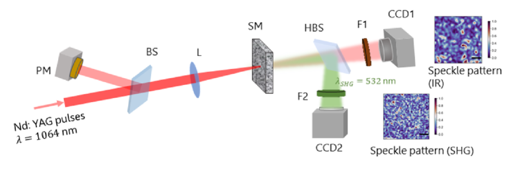
Figure 1: Schematic setup of the experiment. Notations, BS: Beam Splitter, PM: Power Meter, L: Lens , SM: Scattering Medium, HBS: Harmonic Beam Splitter, F1: Laser line filter at $\lambda=$1064\text{\,}\mathrm{n}\mathrm{m}$$, F2: Laser line filter at $\lambda=$532\text{\,}\mathrm{n}\mathrm{m}$$, CCD1: Charged Coupled Device with InGaAs detector, CCD2: Charged Coupled Device with Silicon detector. Two experimental speckle patterns for fundamental (hereafter referred to as IR, $\lambda=$1064\text{\,}\mathrm{n}\mathrm{m}$$) and second harmonic generated (hereafter referred to as SHG, $\lambda=$532\text{\,}\mathrm{n}\mathrm{m}$$) light are shown here while the adjacent color bars indicate the normalized intensity scale.

One of the most fundamental effects in disorder that depends on the phase of the propagating light is the appearance of speckle. A speckle pattern is the random intensity distribution of bright and dark spots developed due to the interference of many coherent wavelets with the same frequency and different amplitudes and phases travelling in a disordered medium [14]. Despite the apparent complete randomness in the intensity distribution, various correlations [15] are known to exist in the speckle pattern. For instance, the optical memory effect ’remembers’ the incoming wavefront under slight perturbation in position and angle [16, 17, 18, 19, 20], an idea that has emerged as an efficient tool in imaging through opaque media [21, 22]. Recent theory and experiments have unveiled non-Gaussian and long-range correlations between transmitted and reflected speckle patterns [23, 24, 25]. Not surprisingly, the rich physics of speckle correlations has already motivated research in nonlinear systems. For instance, a nonlinear optical memory effect [26] was revealed in a $\chi^{(3)}$ medium, namely a silica aerogel, through a series of pump and probe experiments wherein disordered medium is agitated by an optothermal nonlinearity. Another well-known consequence of $\chi^{(3)}$ nonlinearity is the speckle instability, wherein the speckle pattern fluctuates and becomes unstable when the nonlinearity surpasses a threshold value [27, 28, 29]. In the weak localization regime, the speckle patterns formed by nonlinear point scatterers exhibit a dynamic instability and lead to chaotic behavior of the system [30]. Such speckle instabilities in $\chi^{(3)}$ nonlinear disordered media have been experimentally reported [31]. On the other hand, $\chi^{(2)}$ nonlinearity has been employed to primarily investigate angular correlations in speckles. For example, experiments and calculations have shown that angular correlations in reflected speckle scale with sample thickness for second-harmonic light, in contrast to scaling with mean free path for fundamental light [32]. In another study  [33], angular correlations in second-harmonic speckle under dual-beam excitation were presented in a medium of LiNbO_3 microcrystals.

In this article, we report our experimental and theoretical studies on intensity-dependent decorrelation in speckle patterns produced by a second-order nonlinear disordered medium. Specifically, we show that the fundamental and second harmonic speckle patterns produced by successive incident pulses exhibit strong correlations at low input power which drop at higher power. The correlation between fundamental speckle patterns remains high compared to the second harmonic. The decay rate of the average correlation with increasing power is larger in the second harmonic speckles than in the fundamental speckles. To understand the decorrelation process, we build a theoretical model that traces the propagation of the linear field, followed by the conversion to second harmonic, finally followed by the propagation of the second harmonic. The model is in excellent qualitative agreement with the experimental results. The theoretical model is also backed up with a Monte Carlo computation, which sheds light on two contributions to the decorrelation process, namely, the decorrelation during the generation of the second-harmonic, and that due to the propagation thereof.

I Experiments

I.1 Experimental Setup

Towards the experiment, commercially available KDP (Potassium Dihydrogen Phosphate, $@$ EMSURE ACS) crystal grains were adopted as our nonlinear material. Initially, the grain sizes ranged from $\sim\text{$2\text{\,}\mathrm{m}\mathrm{m}3\text{\,}\mathrm{m}\mathrm{m}$}$ and were uneven in shape. The grains were subjected to a ball milling process creating a fine powder of KDP, with particle sizes ranging from $2$ to $8\text{\,}\mathrm{\SIUnitSymbolMicro m}$. The distribution of grain sizes approximately followed a log-normal distribution with a peak at $3.11\text{\,}\mathrm{\SIUnitSymbolMicro m}$ and variance of $1.25\text{\,}\mathrm{\SIUnitSymbolMicro m}$. For the speckle measurement, we prepared two opaque slabs (thickness $\sim\text{$510\pm 15\text{\,}\mathrm{\SIUnitSymbolMicro m}$}$ and $\sim\text{$680\pm 20\text{\,}\mathrm{\SIUnitSymbolMicro m}$}$) of KDP micro-crystals, and the slabs were sandwiched between two microscopic slides of thickness $\sim\text{$170\pm 5\text{\,}\mathrm{\SIUnitSymbolMicro m}$}$. A coherent backscattering (CBS) [34, 35] experiment estimated the transport mean free path ($\ell_{t}$) of the slabs, and the estimated values were approximately $352\text{\,}\mathrm{\SIUnitSymbolMicro m}$ and $169\text{\,}\mathrm{\SIUnitSymbolMicro m}$ at $\lambda=$1064\text{\,}\mathrm{n}\mathrm{m}$$ and $\lambda=$532\text{\,}\mathrm{n}\mathrm{m}$$ respectively. Fig. 1 illustrates the schematic of the experimental setup for the speckle correlations measurements.

Nd:YAG laser pulses (EKSPLA, PL2143B, pulse width $\sim$30\text{\,}\mathrm{p}\mathrm{s}$$) with the fundamental wavelength of $\lambda=$1064\text{\,}\mathrm{n}\mathrm{m}$$ (hereafter referred to as IR), were chosen as our input beam. A glass wedge was introduced in the incident path to direct a small fraction ($\sim$4\text{\,}\%$$) of the beam to a power meter (PM, Ophir Optronics, resolution: $10\text{\,}\mathrm{\SIUnitSymbolMicro}\mathrm{W}$) for the input power measurement. The residual beam was then focused onto the scattering medium (SM) through a lens (L) of focal length $10\text{\,}\mathrm{c}\mathrm{m}$. To avoid damage to the sample, it was placed slightly away from the focus. The transmitted light consisted of both the fundamental and second harmonic light (here referred to as SHG, $\lambda=$532\text{\,}\mathrm{n}\mathrm{m}$$). A harmonic beam splitter (HBS) was employed to separate out the two components. The transmitted (IR) and reflected (SHG) lights from the HBS were then directed to the CCD1 and CCD2 respectively. The CCD1 was an InGaAs detector (SWIR camera, Photonic Science, UK) with pixel dimension 30 x 30 while the CCD2 was a silicon detector (iXon Ultra 897, Andor technology) with pixel dimension 16 x 16. A laser line filter (F1) at $\lambda=$1064\text{\,}\mathrm{n}\mathrm{m}$$ was added in front of the CCD1 to block any unwanted SHG photon. Similarly, a laser line filter (F2) at $\lambda=$532\text{\,}\mathrm{n}\mathrm{m}$$ was placed in front of the CCD2. The laser fired at a repetition rate of $1\text{\,}\mathrm{H}\mathrm{z}$, and simultaneous measurements of the pulse power and the corresponding IR and SHG speckle patterns were made.

I.2 Results

An intense pulse of laser light impacts the disordered sample and imparts certain radiation pressure, which causes the particles to be displaced from their original position. Overall, the disorder configuration at the input face is modified, in proportion to the pump power. See Supplemental Document, Sec. I for details. Since the disorder configuration changes with every impacting optical pulse, it is imperative to avoid cumulative reconfigurations happening through multiple pump pulses. Therefore, we only grab two successive speckle patterns in two consecutive pump pulses, and then translate the sample so as to illuminate a different location on the sample. The homogeneity of disorder strength was constant across the total area, as also certified by the systematic variation in the results. The correlation coefficient between two speckle patterns $A$ and $B$ (both $m\times n$ matrices) was calculated as

$$\mathcal{C}_{\text{expe}}=\frac{\sum_{i=1}^{m}\sum_{j=1}^{n}(A_{ij}-\overline{A})(B_{ij}-\overline{B})}{\sqrt{(\sum_{i=1}^{m}\sum_{j=1}^{n}(A_{ij}-\overline{A})^{2})(\sum_{i=1}^{m}\sum_{j=1}^{n}(B_{ij}-\overline{B})^{2})}}.$$ (1)

where the over-bar represents the mean of the matrix.

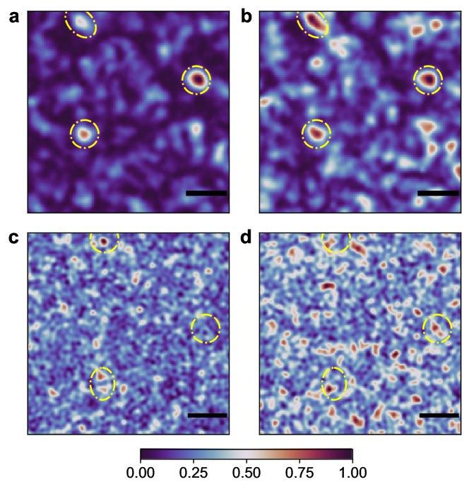
Figure 2: Initial two consecutive speckle patterns of IR [(a) and (b)] and SHG [(c) and (d)] scattered from a $510\text{\,}\mathrm{\SIUnitSymbolMicro m}$ thick sample at an input power of $10.53\text{\,}\mathrm{m}\mathrm{W}$. IR speckle shows higher correlation (0.71), and the marked regions with yellow circles emphasize the agreement. On the contrary, the correlation for SHG light is observed to be low (0.23), and any regions arbitrarily chosen in the pattern (yellow circles) do not show visible agreement. Color bar indicates normalized intensity. The scale bar represents $600\text{\,}\mathrm{\SIUnitSymbolMicro m}$.

Initial two consecutive speckle patterns of IR and SHG at an input power of $10.5\text{\,}\mathrm{m}\mathrm{W}$ are presented in Fig. 2 (a,b) and (c,d) respectively. Obvious agreement between (a) and (b) is seen, with the yellow circles emphasizing the regions of clear similarity. For the SHG wavelength, there are no similarities in the speckle patterns between two consecutive pulses, indicating strong decorrelation within two pulses. The correlation coefficient $\langle\mathcal{C}_{\text{expe}}\rangle$ was averaged over 10 sets of speckle patterns, each grabbed at a different location on the sample at the same pump intensity.

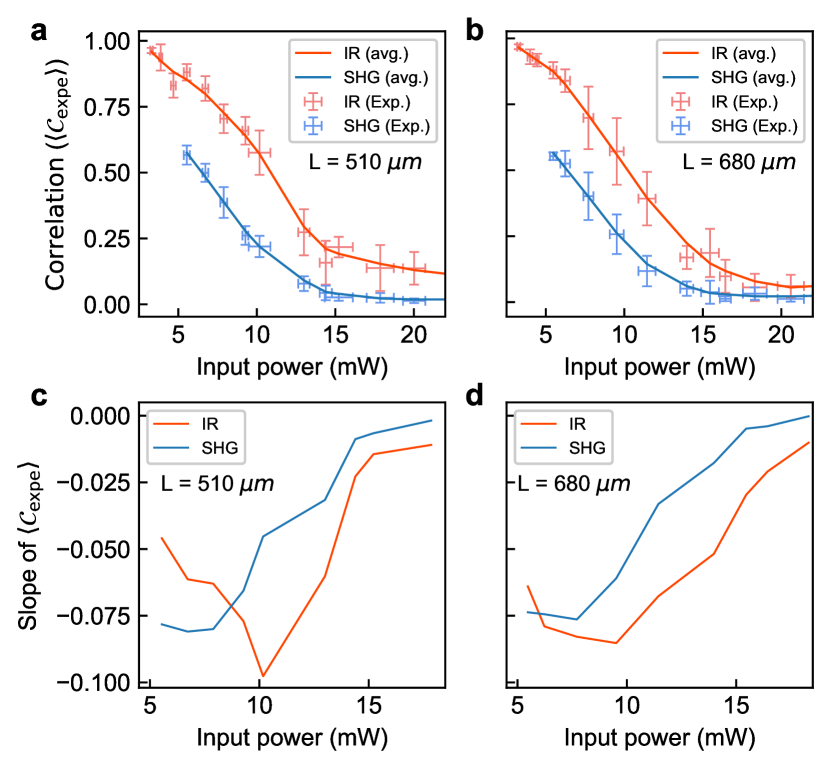
Figure 3: Correlation coefficient between first two consecutive speckle patterns of IR (red markers) and SHG (blue markers) light as a function of input power of the fundamental light, calculated from measured speckle patterns. The solid lines are obtained after smoothing the experimental data. The data are measured on two different samples with thickness $L=$510\text{\,}\mathrm{\SIUnitSymbolMicro m}$$ (a) and $L=$680\text{\,}\mathrm{\SIUnitSymbolMicro m}$$ (b). Slopes of $\langle\mathcal{C}_{\text{expe}}\rangle_{\text{IR}}$ and $\langle\mathcal{C}_{\text{expe}}\rangle_{\text{SHG}}$ calculated on each power value for the two samples are shown in (c) for $L=$510\text{\,}\mathrm{\SIUnitSymbolMicro m}$$ and (d) for $L=$680\text{\,}\mathrm{\SIUnitSymbolMicro m}$$.

Figure 3 reveals the variant decorrelation with pump power for the fundamental and second-harmonic light. A monotonic decrease in the correlation coefficient is observed in both samples of thicknesses $L=$510\text{\,}\mathrm{\SIUnitSymbolMicro m}$$ and $L=$680\text{\,}\mathrm{\SIUnitSymbolMicro m}$$. At low powers, up to about 15 mW, the correlation drops rapidly, where-after the rate reduces with further increase in power. It can be expected to asymptotically approach zero. To compare the qualitative rate of decorrelation between IR and SHG, we calculate the slopes of the two curves for each point and plot them in Fig. 3 (c). For $L=$510\text{\,}\mathrm{\SIUnitSymbolMicro m}$$ and IR light, the slope initially drops indicating a slowing down of the decorrelation with increasing power. Subsequently, it rises monotonically. For the SHG light, an initially static slope is seen to rise monotonically and then saturate at highest power. For the thicker sample, the trends are very similar. The intersection between the blue and red curves indicates the pump power where the decorrelation rates are same. Evidently, the two curves intersect at a lower pump power for the thicker sample. The slopes of the two curves represent the valuable diagnostic for comparing with the theoretical model, which is discussed later.

The source of the fluctuating speckle pattern can be traced to the radiation pressure of the incident pulses, which induces displacements in the scatterers in random directions. This was experimentally verified in our earlier study wherein we showed the decrease in speckle contrast with pump power [36]. A given absolute displacement of the scatterers amounts to a smaller relative displacement with respect to the wavelength for the IR light, as compared to the SHG light. However, the origin of the behavior of decorrelation seen in Figure 3 is not obvious, and needs to be rigorously evaluated. This is carried out in the next section.

II Theoretical Model

In parallel to the experiment, we have developed a theoretical model based on coupled transport equations for the linear ($\lambda=$1064\text{\,}\mathrm{n}\mathrm{m}$$) and second harmonic ($\lambda=$532\text{\,}\mathrm{n}\mathrm{m}$$) lights. This model provides physical insights on the origin of the faster decorrelation for the second harmonic speckle compared to the decorrelation of the linear speckle. Before deriving the model, we first focus on the correlation function defined in Eq. (1). It can also be written as

$$\mathcal{C}_{\text{expe}}=\frac{\int_{\text{CCD}}\delta I(\boldsymbol{\mathbf{r}})\delta\tilde{I}(\boldsymbol{\mathbf{r}})\mathrm{d}\boldsymbol{\mathbf{r}}}{\left[\int_{\text{CCD}}\delta I^{2}(\boldsymbol{\mathbf{r}})\mathrm{d}\boldsymbol{\mathbf{r}}\int_{\text{CCD}}\delta\tilde{I}^{2}(\boldsymbol{\mathbf{r}})\mathrm{d}\boldsymbol{\mathbf{r}}\right]^{1/2}}$$ (2)

where $\delta I=I-\bar{I}$, $I$ being the intensity and $\bar{I}=\int_{\text{CCD}}I(\boldsymbol{\mathbf{r}})\mathrm{d}\boldsymbol{\mathbf{r}}$. $\tilde{I}$ denotes the intensity once the scatterers have moved due to radiation pressure. It is important to note that this correlation function does not correspond to the correlation of speckle patterns at different times but measures the correlation between the speckles produced by two slightly different disorder configurations, the scatterer displacements being induced by the radiation pressure effect. Assuming ergodicity, we can replace the integration over the pixels of the CCD camera by a statistical average over all possible disorder configurations which is denoted by $\left\langle\cdot\right\rangle$. Moreover, we consider that the statistical properties of the medium are the same after the displacements of the scatterers, i.e. $\left\langle I\right\rangle=\left\langle\tilde{I}\right\rangle$. Next, we assume that the field has Gaussian statistics (or equivalently that the speckles are fully developed), which is valid in the regime $k_{0}\ell_{s}\gg 1$, $k_{0}=\omega/c=2\pi/\lambda$ being the wave number and $\ell_{s}$ the scattering mean-free path. This implies that $\left\langle\delta I^{2}\right\rangle=\left\langle I\right\rangle^{2}$. The correlation function in Eq. (2) becomes $\mathcal{C}_{\text{expe}}\sim\mathcal{C}_{I}-1$ where

$$\mathcal{C}_{I}(\boldsymbol{\mathbf{r}})=\frac{\left\langle I(\boldsymbol{\mathbf{r}})\tilde{I}(\boldsymbol{\mathbf{r}})\right\rangle}{\left\langle I(\boldsymbol{\mathbf{r}})\right\rangle^{2}}.$$ (3)

Finally, we also have $\mathcal{C}_{I}=1+|\mathcal{C}|^{2}$ where $\mathcal{C}$ is the field-field correlation function given by

$$\mathcal{C}(\boldsymbol{\mathbf{r}})=\frac{\left\langle E(\boldsymbol{\mathbf{r}})\tilde{E}^{*}(\boldsymbol{\mathbf{r}})\right\rangle}{\left\langle E(\boldsymbol{\mathbf{r}})E^{*}(\boldsymbol{\mathbf{r}})\right\rangle},$$ (4)

$E$ being the electric field and the superscript $*$ denoting the complex conjugate. It is important to note that we make the assumption of a scalar field for the sake of simplicity. This can be justified in the multiple scattering regime where the field can be considered to be fully depolarized [37]. We finally have

$$\mathcal{C}_{\text{expe}}\sim|\mathcal{C}|^{2}.$$ (5)

The problem of estimating theoretically $\mathcal{C}_{\text{expe}}$ now reduces to the computation of $\mathcal{C}$ for two different frequencies, i.e. $\omega$ for the linear beam and $2\omega$ for the second harmonic one. The purpose of the next subsections is to develop a transport model for $\mathcal{C}$. We present only the important steps, the full derivation from first principles being described in the Supplemental Document, Sec. II.

II.1 Disorder model

The real samples are composed of packed KDP crystal grains of different sizes and shapes. Thus the most relevant and simple disorder model consists in a fluctuating continuous and real (no absorption) permittivity $\epsilon(\boldsymbol{\mathbf{r}})$. The disorder microstructure is then characterized by a spatial correlation function chosen to be Gaussian, in the form

$$C_{\epsilon}(|\boldsymbol{\mathbf{r}}-\boldsymbol{\mathbf{r}}^{\prime}|,\omega)=\left\langle\delta\epsilon(\boldsymbol{\mathbf{r}},\omega)\delta\epsilon(\boldsymbol{\mathbf{r}}^{\prime},\omega)\right\rangle\\ =|\Delta\epsilon(\omega)|^{2}\exp\left[-\frac{|\boldsymbol{\mathbf{r}}-\boldsymbol{\mathbf{r}}^{\prime}|^{2}}{2\ell^{2}}\right].$$ (6)

In this equation, $\delta\epsilon(\boldsymbol{\mathbf{r}},\omega)=\epsilon(\boldsymbol{\mathbf{r}},\omega)-\left\langle\epsilon(\boldsymbol{\mathbf{r}},\omega)\right\rangle$ is the fluctuating part of the permittivity, $|\Delta\epsilon(\omega)|^{2}$ is the amplitude of the correlation and $\ell$ is the correlation length. $|\Delta\epsilon(\omega)|^{2}$ depends on frequency since the permittivity $\epsilon$ is dispersive. However, $\ell$ involves only the geometrical structure of the disorder and thus does not depend on frequency. The $\chi^{(2)}$ nonlinearity is supposed to be correlated in a similar way.

II.2 Linear regime

We first consider the linear regime ($\lambda=$1064\text{\,}\mathrm{n}\mathrm{m}$$) correspnding to propagation at the fundamental frequency $\omega$. We use an approach similar to that in Ref. [38] developed in the context of the Diffusing-Wave Spectroscopy (DWS). The most important point concerns the selections of the scattering paths followed by the field $E$ and its complex conjugate $\tilde{E}^{*}$ that dominate in the expression of the correlation function $\mathcal{C}$. In a dilute medium such that $k_{0}\ell_{s}\gg 1$, the leading contribution corresponds to $E$ and $\tilde{E}^{*}$ following the same scattering sequences. These sequences can be represented by the diagram

(7)

with an arbitrary number of scattering events [39]. In these so-called ladder diagrams, the circles represent the scattering events, the thick solid lines correspond to the Green functions modelling the field propagation between scattering events and the thick dashed lines denote the incident field. The upper (bottom) line describes the propagation of $E$ ($\tilde{E}^{*}$) respectively and the thin dashed vertical lines represent the disorder correlation $C$. It is important to note that in the model of continuous disorder, the circles do not represent real scatterers (grains) but scattering events connected by the correlation function $C$. The width $\ell$ of the correlation function $C$ is however on the order of the grain size. The ladder shape of this dominant diagram implies that there is always constructive interference between the field $E$ and its complex conjugate $\tilde{E}^{*}$. Thus the problem of computation of $\mathcal{C}$ reduces to the problem of solving a radiative transport equation [40]

$$\left[\boldsymbol{\mathbf{u}}\cdot\boldsymbol{\mathbf{\nabla}}_{\boldsymbol{\mathbf{r}}}+\frac{1}{\ell_{s}(\omega)}\right]\tilde{I}(\boldsymbol{\mathbf{r}},\boldsymbol{\mathbf{u}},\omega)\\ =\frac{1}{\ell_{s}(\omega)}\int p(\boldsymbol{\mathbf{u}},\boldsymbol{\mathbf{u}}^{\prime},\omega)g(\boldsymbol{\mathbf{r}},\boldsymbol{\mathbf{u}},\boldsymbol{\mathbf{u}}^{\prime},\omega)\tilde{I}(\boldsymbol{\mathbf{r}},\boldsymbol{\mathbf{u}}^{\prime},\omega)\mathrm{d}\boldsymbol{\mathbf{u}}^{\prime}.$$ (8)

where $\tilde{I}(\boldsymbol{\mathbf{r}},\boldsymbol{\mathbf{u}},\omega)$ is the specific intensity, that can be seen as the radiative flux at position $\boldsymbol{\mathbf{r}}$, in direction $\boldsymbol{\mathbf{u}}$ and at frequency $\omega$. More precisely, it can be shown from first principles that it is given by the Wigner transform of the field. In our context (scatterer displacements), it reads

$$\delta(k-k_{0})\tilde{I}(\boldsymbol{\mathbf{r}},\boldsymbol{\mathbf{u}},\omega)=\int\left\langle E\left(\boldsymbol{\mathbf{r}}+\frac{\boldsymbol{\mathbf{s}}}{2},\omega\right)\tilde{E}^{*}\left(\boldsymbol{\mathbf{r}}-\frac{\boldsymbol{\mathbf{s}}}{2},\omega\right)\right\rangle\\ \times e^{-ik\boldsymbol{\mathbf{u}}\cdot\boldsymbol{\mathbf{s}}}\mathrm{d}\boldsymbol{\mathbf{s}}.$$ (9)

Thus, solving for $\tilde{I}$ gives a direct access to the field-field correlation function $\mathcal{C}$. Equation (8) is very similar to the standard Radiative Transfer Equation (RTE) [41] except that it includes an additional function $g(\boldsymbol{\mathbf{r}},\boldsymbol{\mathbf{u}},\boldsymbol{\mathbf{u}}^{\prime},\omega)$ that represents the decorrelation of the field at each scattering event due to the motion of scatterers. It is given by

$$g(\boldsymbol{\mathbf{r}},\boldsymbol{\mathbf{u}},\boldsymbol{\mathbf{u}}^{\prime},\omega)=\int e^{-ik_{0}(\boldsymbol{\mathbf{u}}-\boldsymbol{\mathbf{u}}^{\prime})\cdot\boldsymbol{\mathbf{\Delta}}}f(\boldsymbol{\mathbf{r}},\boldsymbol{\mathbf{\Delta}})\mathrm{d}\boldsymbol{\mathbf{\Delta}}$$ (10)

where $\boldsymbol{\mathbf{u}}$ and $\boldsymbol{\mathbf{u}}^{\prime}$ are unit vectors representing the scattered and incoming directions for a given scattering process. $f(\boldsymbol{\mathbf{r}},\boldsymbol{\mathbf{\Delta}})$ is the probability density to have a displacement $\boldsymbol{\mathbf{\Delta}}$ of a scatterer at the position $\boldsymbol{\mathbf{r}}$. The position dependence is required since this displacement is induced by the radiation pressure that can be heterogeneous inside the medium (in particular at small depths). Eq. (10) can be interpreted as follows: the decorrelation is due to the phase shift (Doppler shift) averaged over all accessible displacements for a scatterer. As a simple model, we consider that the amplitude of the displacement is proportional to the specific intensity which leads to

$$f\left(\boldsymbol{\mathbf{r}},\boldsymbol{\mathbf{\Delta}}\right)=\delta\left[\Delta-\beta I\left(\boldsymbol{\mathbf{r}},\frac{\boldsymbol{\mathbf{\Delta}}}{\Delta},\omega\right)\right]\\ \times\left[\beta^{2}\int I\left(\boldsymbol{\mathbf{r}},\boldsymbol{\mathbf{u}},\omega\right)^{2}\mathrm{d}{\boldsymbol{\mathbf{u}}}\right]^{-1}$$ (11)

where $\beta$ is factor taking into account the link between the displacement and the value of the specific intensity. In the following $\beta$ will be considered as a scaling parameter. In Eq. (11), $I\left(\boldsymbol{\mathbf{r}},\boldsymbol{\mathbf{u}},\omega\right)$ is the specific intensity without any displacements. Finally $p(\boldsymbol{\mathbf{u}},\boldsymbol{\mathbf{u}}^{\prime},\omega)$ is the phase function representing the part of energy incident from direction $\boldsymbol{\mathbf{u}}^{\prime}$ and scattered into direction $\boldsymbol{\mathbf{u}}$. For the Gaussian disorder considered here, it is given by

$$p(\boldsymbol{\mathbf{u}},\boldsymbol{\mathbf{u}}^{\prime},\omega)\propto\mathcal{p}(k_{0}|\boldsymbol{\mathbf{u}}-\boldsymbol{\mathbf{u}}^{\prime}|)\quad\text{where}\quad\mathcal{p}(q)=\exp\left[-\frac{q^{2}\ell^{2}}{2}\right]$$ (12)

and normalized such that $\int p(\boldsymbol{\mathbf{u}},\boldsymbol{\mathbf{u}}^{\prime},\omega)\mathrm{d}\boldsymbol{\mathbf{u}}^{\prime}=1$. Equation (8) can easily be interpreted using a random walk approach. Indeed, light undergoes a random walk whose average step is given by the scattering mean-free path $\ell_{s}(\omega)$ and whose angular distribution at each scattering event is given by the phase function $p(\boldsymbol{\mathbf{u}},\boldsymbol{\mathbf{u}}^{\prime},\omega)$. A phase shift is introduced between the fields at each scattering event due to the displacement of the scatterers as described by the function $g(\boldsymbol{\mathbf{r}},\boldsymbol{\mathbf{u}},\boldsymbol{\mathbf{u}}^{\prime},\omega)$.

II.3 Second harmonic regime

We now address the question of the generation and propagation of the second harmonic light. As it is usually done in homogeneous materials, we use a perturbative approach in order to compute the field at $2\omega$ from the field at $\omega$. The full process can be broken down into three steps. First the linear field at $\omega$ propagates inside the material. Second, it is converted to second harmonic on an arbitrary scatterer. And finally, this process is followed by the propagation of the second harmonic field. The same sequence of processes also applies to the complex conjugate of the field. From this sequence, the most important point is still here the identification of the leading diagram taking into account the non-linearity. It is given by

(13)

where the squares represent the second harmonic generation process. We could assume the non-linear processes for $E$ and $\tilde{E}^{*}$ to occur at two positions with an arbitrary distance between them. However, this would lead to the propagation of the correlations $\left\langle E(\boldsymbol{\mathbf{r}},\omega)\tilde{E}^{*}(\boldsymbol{\mathbf{r}},2\omega)\right\rangle$ or $\left\langle E(\boldsymbol{\mathbf{r}},2\omega)\tilde{E}^{*}(\boldsymbol{\mathbf{r}},\omega)\right\rangle$ which are supposed to vanish since they involve fields at two different frequencies. The generations of the second harmonic sources for $E$ and $\tilde{E}^{*}$ are then confined in a small volume with typical size $\ell$. The relevance of the dominant diagram responsible for the second harmonic correlation has to be carefully checked. For that purpose, we have performed ab initio numerical simulations that are presented in the Supplemental Document, Sec. III. Finally, the diagram of Eq. (13) can be interpreted the following way: the right part represents the propagation of two specific intensities at frequency $\omega$ obeying Eq. (8) and the left part represents the propagation of the specific intensity at frequency $2\omega$. It is given by the following non-linear RTE

$$\left[\boldsymbol{\mathbf{u}}\cdot\boldsymbol{\mathbf{\nabla}}_{\boldsymbol{\mathbf{r}}}+\frac{1}{\ell_{s}(2\omega)}\right]\tilde{I}(\boldsymbol{\mathbf{r}},\boldsymbol{\mathbf{u}},2\omega)\\ =\frac{1}{\ell_{s}(2\omega)}\int p(\boldsymbol{\mathbf{u}},\boldsymbol{\mathbf{u}}^{\prime},2\omega)g(\boldsymbol{\mathbf{r}},\boldsymbol{\mathbf{u}},\boldsymbol{\mathbf{u}}^{\prime},2\omega)\tilde{I}(\boldsymbol{\mathbf{r}},\boldsymbol{\mathbf{u}}^{\prime},2\omega)\mathrm{d}\boldsymbol{\mathbf{u}}^{\prime}\\ +\alpha\iint p_{\text{SHG}}(\boldsymbol{\mathbf{u}},\boldsymbol{\mathbf{u}}^{\prime},\boldsymbol{\mathbf{u}}^{\prime\prime},\omega)g_{\text{SHG}}(\boldsymbol{\mathbf{r}},\boldsymbol{\mathbf{u}},\boldsymbol{\mathbf{u}}^{\prime},\boldsymbol{\mathbf{u}}^{\prime\prime},\omega)\\ \times\tilde{I}(\boldsymbol{\mathbf{r}},\boldsymbol{\mathbf{u}}^{\prime},\omega)\tilde{I}(\boldsymbol{\mathbf{r}},\boldsymbol{\mathbf{u}}^{\prime\prime},\omega)\mathrm{d}\boldsymbol{\mathbf{u}}^{\prime}\mathrm{d}\boldsymbol{\mathbf{u}}^{\prime\prime}.$$ (14)

This equation is the main theoretical result of this work. It shows that the second harmonic specific intensity follows a similar transport equation as the fundamental intensity [Eq. (8)], but with a source term describing the non-linear conversion process. Its physical interpretation is very simple: Light propagates first at frequency $\omega$ which is described by the specific intensity $\tilde{I}(\boldsymbol{\mathbf{r}},\boldsymbol{\mathbf{u}}^{\prime\prime},\omega)$ solution to Eq. (8). Then a SHG process occurs which creates a source at frequency $2\omega$, the amplitude of which is given by the product of two specific intensities at $\omega$. Finally, propagation at $2\omega$ is described by the specific intensity $\tilde{I}(\boldsymbol{\mathbf{r}},\boldsymbol{\mathbf{u}}^{\prime\prime},2\omega)$ that follows Eq. (14). In this expression, $\alpha$ is a factor that takes into account all constants involved in the SHG process such as $\chi^{(2)}$. $p_{\text{SHG}}(\boldsymbol{\mathbf{u}},\boldsymbol{\mathbf{u}}^{\prime},\boldsymbol{\mathbf{u}}^{\prime\prime},\omega)$ is the SHG phase function. It involves three units vectors. $\boldsymbol{\mathbf{u}}^{\prime}$ and $\boldsymbol{\mathbf{u}}^{\prime\prime}$ corresponds to the incoming directions of the two specific intensities at $\omega$ and $\boldsymbol{\mathbf{u}}$ is the outgoing direction of the specific intensity at 2$\omega$. In the case of the correlated disorder we consider here, we have

$$p_{\text{SHG}}(\boldsymbol{\mathbf{u}},\boldsymbol{\mathbf{u}}^{\prime},\boldsymbol{\mathbf{u}}^{\prime\prime},\omega)\propto\mathcal{p}(k_{0}|2\boldsymbol{\mathbf{u}}-\boldsymbol{\mathbf{u}}^{\prime}-\boldsymbol{\mathbf{u}}^{\prime\prime}|)$$ (15)

with $\int p_{\text{SHG}}(\boldsymbol{\mathbf{u}},\boldsymbol{\mathbf{u}}^{\prime},\boldsymbol{\mathbf{u}}^{\prime\prime},\omega)\mathrm{d}\boldsymbol{\mathbf{u}}^{\prime}\mathrm{d}\boldsymbol{\mathbf{u}}^{\prime\prime}=1$. $\boldsymbol{\mathbf{u}}$ appears with a factor two since it corresponds to the non-linear specific intensity direction. $g_{\text{SHG}}(\boldsymbol{\mathbf{u}},\boldsymbol{\mathbf{u}}^{\prime},\boldsymbol{\mathbf{u}}^{\prime\prime},\omega)$ is the decorrelation function given by

$$g_{\text{SHG}}(\boldsymbol{\mathbf{r}},\boldsymbol{\mathbf{u}},\boldsymbol{\mathbf{u}}^{\prime},\boldsymbol{\mathbf{u}}^{\prime\prime},\omega)=\int e^{-ik_{0}(2\boldsymbol{\mathbf{u}}-\boldsymbol{\mathbf{u}}^{\prime}-\boldsymbol{\mathbf{u}}^{\prime\prime})\cdot\boldsymbol{\mathbf{\Delta}}}f(\boldsymbol{\mathbf{r}},\boldsymbol{\mathbf{\Delta}})\mathrm{d}\boldsymbol{\mathbf{\Delta}}.$$ (16)

It still corresponds to the decorrelation induced by a Doppler shift involving three beams, i.e. two incoming beams at frequency $\omega$ in directions $\boldsymbol{\mathbf{u}}^{\prime}$ and $\boldsymbol{\mathbf{u}}^{\prime\prime}$ and one outgoing beam at frequency $2\omega$ in direction $\boldsymbol{\mathbf{u}}$.

II.4 Numerical simulations

In order, to solve the system of Eqs. (8) and (14), we have developed a Monte Carlo scheme which can be seen as a random walk process inside the material [42]. Three Monte Carlo simulations are performed in a slab geometry of thickness $L$ under plane-wave illumination at normal incidence. The first is used to compute $I\left(\boldsymbol{\mathbf{r}},\boldsymbol{\mathbf{u}},\omega\right)$, the specific intensity in the absence of displacement of the scatterers. This is required in order to compute the probability density $f(\boldsymbol{\mathbf{r}},\boldsymbol{\mathbf{\Delta}})$ to have a displacement $\boldsymbol{\mathbf{\Delta}}$ at position $\boldsymbol{\mathbf{r}}$. The second Monte Carlo simulation is used to compute $\tilde{I}\left(\boldsymbol{\mathbf{r}},\boldsymbol{\mathbf{u}},\omega\right)$, the specific intensity associated with the correlation function at $\omega$. Finally, a last simulation is performed in order to compute $\tilde{I}\left(\boldsymbol{\mathbf{r}},\boldsymbol{\mathbf{u}},2\omega\right)$, the specific intensity associated with the correlation function at $2\omega$. More precisely, the correlation functions are computed from the energy density at the output interface in transmission, i.e.

$$\mathcal{C}(\omega) =\frac{\int\tilde{I}\left(z=L,\boldsymbol{\mathbf{u}},\omega\right)\mathrm{d}\boldsymbol{\mathbf{u}}}{\int I\left(z=L,\boldsymbol{\mathbf{u}},\omega\right)\mathrm{d}\boldsymbol{\mathbf{u}}},$$ (17)

$$\mathcal{C}(2\omega) =\frac{\int\tilde{I}\left(z=L,\boldsymbol{\mathbf{u}},2\omega\right)\mathrm{d}\boldsymbol{\mathbf{u}}}{\int I\left(z=L,\boldsymbol{\mathbf{u}},2\omega\right)\mathrm{d}\boldsymbol{\mathbf{u}}}.$$ (18)

This computations are performed for different incident intensities $I_{0}$ (or different incident powers $\left\langle P\right\rangle$) meaning different probability density $f(\boldsymbol{\mathbf{r}},\boldsymbol{\mathbf{\Delta}})$ which correspond to different radiation pressures. Regarding the numerical parameters, it is important to keep in mind that the KDP powder used in the experiment has crystal grains of different sizes ranging from $2\text{\,}\mathrm{\SIUnitSymbolMicro m}$ to $8\text{\,}\mathrm{\SIUnitSymbolMicro m}$. This makes difficult the choice of the correlation length $\ell$. However we have tested several values showing that this is not a crucial parameter. Since the particles are large compared to the wavelength, we have chosen $k_{0}\ell=3$ for the results presented in Fig. 4. This gives the anisotropy factors $g(\omega)=0.89$ and $g(2\omega)=0.97$. The thickness of the medium $L$ as well as the transport mean-free paths $\ell_{t}=\ell_{s}/(1-g)$ take the values measured experimentally, which gives $k_{0}L=4016$, $k_{0}\ell_{t}(\omega)=2079$ and $k_{0}\ell_{t}(2\omega)=998$. This finally leads to the normalized scattering mean-free paths $k_{0}\ell_{s}(\omega)=229$ and $k_{0}\ell_{s}(2\omega)=30$.

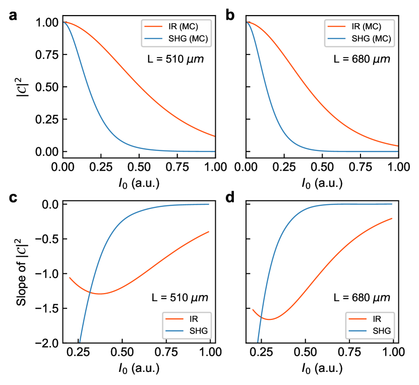
Figure 4: Monte Carlo (MC) simulated correlation functions $|\mathcal{C}|^{2}$ for the linear (red solid line) and second harmonic (blue solid line) beams as a function of the incident intensity $I_{0}$ in arbitrary units. (a) $L=510$ $\mu$m, (b) $L=680$ $\mu$m. The range of $I_{0}$ is chosen such that the extreme values of the linear correlation $|\mathcal{C}(\omega)|^{2}$ are in agreement with the experimental values $\mathcal{C}_{\text{expe}}(\omega)$ presented. Slopes of $|\mathcal{C}(\omega)|^{2}$ and $|\mathcal{C}(2\omega)|^{2}$ calculated on each power value for the two samples are shown in (c) $L=$510\text{\,}\mathrm{\SIUnitSymbolMicro m}$$ and (d) $L=$680\text{\,}\mathrm{\SIUnitSymbolMicro m}$$. A qualitative agreement is immediately seen with the experimental behavior in Fig. 3

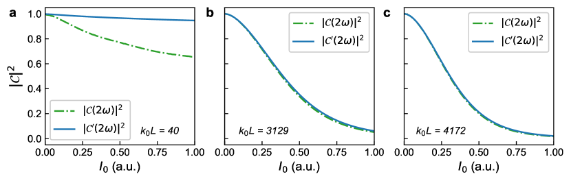
Figure 5: Monte Carlo (MC) simulated correlation functions $|\mathcal{C}|^{2}$ for the second harmonic speckles taking into account all decorrelation effects (i.e. effect of $g$ and $g_{\text{SHG}}$, green dashed line) and only the decorrelation occurring during beam propagation (i.e. effect of $g$, blue solid line). The computations are performed for (a) $k_{0}L=40$, (b) $k_{0}L=3129$ and (c) $k_{0}L=4172$. The other parameters are the same as in Fig. 4.

We can observe that the results shown in Fig. 3 are reproduced qualitatively. The second-harmonic beam decorrelates faster than that of the fundamental frequency. The slopes of the decorrelation curves also reproduce the same trends seen in experiments, for most part of the input power range. The IR light shows a reducing slope followed by a rise at a certain pump power, while the frequency-doubled light shows a steady rise followed by a saturation region. Barring a minor difference at low powers, the experimental data exhibit the same behavior. The crossing of the two slope curves also happens at a lower pump power in the thicker sample, as seen in the experiments. The agreement with the experiments is very clear qualitatively, but is not quantitative. The main reason should probably be investigated in the dependence of the probability density $f$ on the specific intensity $I$. Building this relationship is not a trivial task and is out of the scope of the present work. A second potential effect that has been neglected so far, is the role of the refractive index mismatch at the interfaces of the slab. In the Monte Carlo simulation we have verified that this does not change substantially the results up to a refractive index $n=2$.

The faster decorrelation of the second harmonic speckle can be explained through two different mechanisms: The first one corresponds to the decorrelation when the second harmonic light is generated which is represented by $g_{\text{SHG}}(\boldsymbol{\mathbf{r}},\boldsymbol{\mathbf{u}},\boldsymbol{\mathbf{u}}^{\prime},\boldsymbol{\mathbf{u}}^{\prime\prime},\omega)$. Its dependence on the three different directions through the relation $2\boldsymbol{\mathbf{u}}-\boldsymbol{\mathbf{u}}^{\prime}-\boldsymbol{\mathbf{u}}^{\prime\prime}$ favors a faster decorrelation. The second mechanism is due to the propagation of the second harmonic field. The factor of two in $g(\boldsymbol{\mathbf{r}},\boldsymbol{\mathbf{u}},\boldsymbol{\mathbf{u}}^{\prime},2\omega)$ also makes the correlation vanish faster than for the linear beam. For a small optical thickness, both effects play a role and have to be taken into account properly. This comes from the fact that photons experience few scattering events before escaping the medium and thus the decorrelations due to $g_{\text{SHG}}$ and to $g$ are of the same order of magnitude. On the other hand, for large optical thicknesses, many scattering events are involved and the contribution of $g_{\text{SHG}}$ is negligible compared to that of $g$. Figure 5 illustrate this statement using the Monte Carlo simulations. This simple conclusion will also be easily observed in the more simple case of statistically homogeneous and isotropic displacements discussed in the next section.

II.5 Statistically homogeneous and isotropic displacements

Beyond the effect of radiation pressure that has been examined in this study, it is also interesting to consider a displacement probability for the scatterers that is homogeneous and isotropic, i.e. $f(\boldsymbol{\mathbf{r}},\boldsymbol{\mathbf{\Delta}})=f(\Delta)/(4\pi\Delta^{2})$. Indeed, considering large medium thicknesses compared to the transport mean-free paths, i.e. $L\gg\{\ell_{t}(\omega),\ell_{t}(2\omega)\}$, we can derive diffusion equations for the linear and second harmonic correlation functions. The derivation is detailed in the Supplemental Document, Sec. IV and leads to analytical expressions given by

$$\mathcal{C}(\omega) =\frac{\kappa(\omega)L}{\sinh[\kappa(\omega)L]},$$ (19)

$$\mathcal{C}(2\omega) =\frac{6\mathcal{D}(\omega)}{\kappa(2\omega)L\sinh[\kappa(\omega)L]^{2}\sinh[\kappa(2\omega)L]}$$

$$\times\frac{\kappa(2\omega)^{2}\left\{1-\cosh[2\kappa(\omega)L]\right\}-4\kappa(\omega)^{2}\left\{1-\cosh[\kappa(2\omega)L]\right\}}{\kappa(2\omega)^{2}-4\kappa(\omega)^{2}}$$ (20)

where

$$\kappa =\sqrt{\frac{3}{\tilde{\ell}_{t}\tilde{\ell}_{a}}},\quad\tilde{\ell}_{t}=\frac{\ell_{s}}{1-\tilde{g}},$$ (21)

$$\frac{1}{\tilde{\ell}_{a}} =\frac{1}{\ell_{s}}\left[1-\int p(\boldsymbol{\mathbf{u}},\boldsymbol{\mathbf{u}}^{\prime})g(\boldsymbol{\mathbf{u}},\boldsymbol{\mathbf{u}}^{\prime})\mathrm{d}\boldsymbol{\mathbf{u}}^{\prime}\right],$$ (22)

$$\text{and }\tilde{g} =\frac{\int p(\boldsymbol{\mathbf{u}},\boldsymbol{\mathbf{u}}^{\prime})g(\boldsymbol{\mathbf{u}},\boldsymbol{\mathbf{u}}^{\prime})\boldsymbol{\mathbf{u}}\cdot\boldsymbol{\mathbf{u}}^{\prime}\mathrm{d}\boldsymbol{\mathbf{u}}^{\prime}}{\int p(\boldsymbol{\mathbf{u}},\boldsymbol{\mathbf{u}}^{\prime})g(\boldsymbol{\mathbf{u}},\boldsymbol{\mathbf{u}}^{\prime})\mathrm{d}\boldsymbol{\mathbf{u}}^{\prime}},$$ (23)

all these four quantities being defined at $\omega$ and $2\omega$. We also have

$$\mathcal{D}(\omega)=\frac{\int p_{\text{SHG}}(\boldsymbol{\mathbf{u}},\boldsymbol{\mathbf{u}}^{\prime},\boldsymbol{\mathbf{u}}^{\prime\prime},\omega)g_{\text{SHG}}(\boldsymbol{\mathbf{u}},\boldsymbol{\mathbf{u}}^{\prime},\boldsymbol{\mathbf{u}}^{\prime\prime},\omega)\mathrm{d}\boldsymbol{\mathbf{u}}\mathrm{d}\boldsymbol{\mathbf{u}}^{\prime}\mathrm{d}\boldsymbol{\mathbf{u}}^{\prime\prime}}{\int p_{\text{SHG}}(\boldsymbol{\mathbf{u}},\boldsymbol{\mathbf{u}}^{\prime},\boldsymbol{\mathbf{u}}^{\prime\prime},\omega)\mathrm{d}\boldsymbol{\mathbf{u}}\mathrm{d}\boldsymbol{\mathbf{u}}^{\prime}\mathrm{d}\boldsymbol{\mathbf{u}}^{\prime\prime}}.$$ (24)

We clearly see from these expressions that the effect of the decorrelation during the propagation of the waves at $\omega$ or at $2\omega$ can be seen as an absorption effect and are encoded in the $\kappa$ functions. The decorrelation process taking place during the generation of the second harmonic light is encoded in the $\mathcal{D}$ function. Finally these analytical expressions can be simplified in the even more particular case of isotropic scattering such that $p(\boldsymbol{\mathbf{u}},\boldsymbol{\mathbf{u}}^{\prime})=1/(4\pi)$ and $p_{\text{SHG}}(\boldsymbol{\mathbf{u}},\boldsymbol{\mathbf{u}}^{\prime},\boldsymbol{\mathbf{u}}^{\prime\prime},\omega)=1/(16\pi^{2})$ and of a constant displacement amplitude $d$ such that $k_{0}d\ll 1$ and $f(\Delta)=\delta(\Delta-d)$. This gives

$$\kappa(\omega)L =b(\omega)k_{0}d,\quad\kappa(2\omega)L=2b(2\omega)k_{0}d$$ (25)

$$\text{and }\mathcal{D}(\omega) =\frac{1}{8\pi}\int_{\phi=0}^{2\pi}\int_{\mu=-1}^{1}\int_{\mu^{\prime}=-1}^{1}\operatorname{sinc}\left[k_{0}d\vphantom{\sqrt{6-4\mu-4\mu^{\prime}+2\mu\mu^{\prime}+2\sqrt{1-\mu^{2}}\sqrt{1-\mu^{\prime 2}}\cos\phi}}\right.$$

$$\left.\times\sqrt{6-4\mu-4\mu^{\prime}+2\mu\mu^{\prime}+2\sqrt{1-\mu^{2}}\sqrt{1-\mu^{\prime 2}}\cos\phi}\right]$$

$$\times\mathrm{d}\mu\mathrm{d}\mu^{\prime}\mathrm{d}\phi$$ (26)

where $b=L/\ell_{s}$ is the optical thickness. These last expressions are very useful to get more insights on the decorrelation effects encoded in functions $\kappa(\omega)$, $\kappa(2\omega)$ and $\mathcal{D}(\omega)$. In particular, as already noticed in the numerical simulations, we clearly see that the decorrelation during propagation is stronger when the optical thicknesses $b(\omega)$ and $b(2\omega)$ increase which reduces the effect of $\mathcal{D}(\omega)$. In the diffusive regime considered here, $\mathcal{D}(\omega)$ can thus be replaced by its limit when $k_{0}d\to 0$, i.e. $\mathcal{D}(\omega)\sim 1$.

III Discussion and Conclusion

In summary, we have experimentally investigated the decorrelation of speckle patterns with increasing pump power in a second-order nonlinear disordered medium. Simultaneous speckle measurements at the fundamental and second harmonic wavelengths reveal a varying rate of decorrelation under the same incident power. The decorrelation arises from the microscopic displacements in the disorder configuration induced by the radiation pressure produced by the pump beam. In addition, the second harmonic correlation decreases faster than the fundamental. We laid the foundations of a theoretical model that accurately describes the synergy of second-order nonlinearity and light diffusion. The model demarcates the contribution of two components in the decorrelation, namely, one arising from the generation of second-harmonic light, and the other arising from the propagation thereof. For the samples and input powers employed in our experiments, the former seems to be the stronger contributor. Wider investigations of the model show that the relative strengths of the two components depend upon the degree of disorder. Towards the differences in the experimental and computed results, we have discussed qualitatively the origins as follows. The actual displacement at a location $\boldsymbol{\mathbf{r}}$ is dependent on the specific intensity at that location, and the size and shape of the particle at that location. This is too intricate a parameter to calculate, and we did not venture into it. In the theory, the sample is homogeneously disordered, and particle size is not a parameter in computing the displacement under radiation pressure. At a future stage, a distribution in the displacements may be invoked in the theory. We believe these unavoidable differences in the experimental samples and theoretical assumptions limit the agreement in the respective results. This study shades light on the subtle mechanism of non-linear conversion in disordered media, with expected outcomes in fundamental studies in mesoscopic wave transport, as well as the design of efficient materials for non-linear generation of light.

Funding Information

Department of Atomic Energy, Government of India for funding for the project identification No. RTI4002 under the DAE OM No 1303/1/2020/R&D-II/DAE/5567 dated 20.8.2020; Swarnajayanti Fellowship, Department of Science and Technology, Ministry of Science and Technology, India.

This work has received support under the program “Investissements d’Avenir” launched by the French Government.

Disclosures

The authors declare no conflicts of interest.

References

- Ishimaru [1978] A. Ishimaru, Wave Propagation and Scattering in Random Media (Academic, 1978).
- Wiersma [2013] D. S. Wiersma, Disordered photonics, Nature Photonics 7, 188–196 (2013).
- Conti et al. [2007] C. Conti, L. Angelani, and G. Ruocco, Light diffusion and localization in three-dimensional nonlinear disordered media, Phys. Rev. A 75, 033812 (2007).
- Shadrivov et al. [2010] I. V. Shadrivov, K. Y. Bliokh, Y. P. Bliokh, V. Freilikher, and Y. S. Kivshar, Bistability of anderson localized states in nonlinear random media, Phys. Rev. Lett. 104, 123902 (2010).
- Mafi [2017] A. Mafi, A brief overview of the interplay between nonlinearity and transverse anderson localization, arXiv:1703.04011 (2017).
- Sharabi et al. [2018] Y. Sharabi, H. H. Sheinfux, Y. Sagi, G. Eisenstein, and M. Segev, Self-induced diffusion in disordered nonlinear photonic media, Phys. Rev. Lett. 121, 233901 (2018).
- Agranovich and Kravtsov [1988] V. M. Agranovich and V. E. Kravtsov, Effects of weak localization of photons in nonlinear optics: Second harmonic generation, Physics Letters A 131, 378 (1988).
- Yoo et al. [1989] K. M. Yoo, S. Lee, Y. Takiguchi, and R. R. Alfano, Search for the effect of weak photon localization in second-harmonic waves generated in a disordered anisotropic nonlinear medium, Optics Letters 14, 800 (1989).
- Faez et al. [2009] S. Faez, P. M. Johnson, D. A. Mazurenko, and A. Lagendijk, Experimental observation of second-harmonic generation and diffusion inside random media, Journal of the Optical Society of America B 26, 235 (2009).
- Valencia and Méndez [2009] C. I. Valencia and E. R. Méndez, Weak localization effects in the second-harmonic light scattered by random systems of particles, Optics Communications 282, 1706 (2009).
- Savo et al. [2020] R. Savo, A. Morandi, J. S. Müller, F. Kaufmann, F. Timpu, M. R. Escalé, M. Zanini, L. Isa, and R. Grange, Broadband mie driven random quasi-phase-matching, Nature Photonics 14, 740–747 (2020).
- Müller et al. [2021] J. S. Müller, A. Morandi, R. Grange, and R. Savo, Modeling of random quasi-phase-matching in birefringent disordered media, Physical Review Applied 15, 064070 (2021).
- Morandi et al. [2022] A. Morandi, R. Savo, J. S. Müller, S. Reichen, and R. Grange, Multiple scattering and random quasi-phase-matching in disordered assemblies of LiNbO3 nanocubes, ACS Photonics 9, 1882–1888 (2022).
- Goodman [2007] J. W. Goodman, Speckle Phenomena in Optics: Theory and Applications (Roberts & Company, 2007).
- Feng et al. [1988] S. Feng, C. Kane, P. A. Lee, and A. D. Stone, Correlations and fluctuations of coherent wave transmission through disordered media, Physical Review Letters 61, 834 (1988).
- Freund et al. [1988] I. Freund, M. Rosenbluh, and S. Feng, Memory effects in propagation of optical waves through disordered media, Physical Review Letters 61, 2328 (1988).
- Schott et al. [2015] S. Schott, J. Bertolotti, J.-F. Léger, L. Bourdieu, and S. Gigan, Characterization of the angular memory effect of scattered light in biological tissues, Optics Express 23, 13505 (2015).
- Judkewitz et al. [2015] B. Judkewitz, R. Horstmeyer, I. M. Vellekoop, I. N. Papadopoulos, and C. Yang, Translation correlations in anisotropically scattering media, Nature Physics 11, 684–689 (2015).
- Osnabrugge et al. [2017] G. Osnabrugge, R. Horstmeyer, I. N. Papadopoulos, B. Judkewitz, and I. M. Vellekoop, Generalized optical memory effect, Optica 4, 886 (2017).
- Liu et al. [2019] H. Liu, Z. Liu, M. Chen, S. Han, and L. V. Wang, Physical picture of the optical memory effect, Photonics Research 7, 1323 (2019).
- Bertolotti et al. [2012] J. Bertolotti, E. G. van Putten, C. Blum, A. Lagendijk, W. L. Vos, and A. P. Mosk, Non-invasive imaging through opaque scattering layers, Nature 491, 232–234 (2012).
- Katz et al. [2014] O. Katz, P. Heidmann, M. Fink, and S. Gigan, Non-invasive single-shot imaging through scattering layers and around corners via speckle correlations, Nature Photonics 8, 784–790 (2014).
- Fayard et al. [2015] N. Fayard, A. Cazé, R. Pierrat, and R. Carminati, Intensity correlations between reflected and transmitted speckle patterns, Physical Review A 92, 033827 (2015).
- Fayard et al. [2018] N. Fayard, A. Goetschy, R. Pierrat, and R. Carminati, Mutual information between reflected and transmitted speckle images, Physical Review Letters 120, 073901 (2018).
- Starshynov et al. [2018] I. Starshynov, A. M. Paniagua-Diaz, N. Fayard, A. Goetschy, R. Pierrat, R. Carminati, and J. Bertolotti, Non-gaussian correlations between reflected and transmitted intensity patterns emerging from opaque disordered media, Physical Review X 8, 021041 (2018).
- Fleming et al. [2019] A. Fleming, C. Conti, T. Vettenburg, and A. D. Falco, Nonlinear optical memory effect, Optics Letters 44, 4841 (2019).
- Skipetrov and Maynard [2000] S. E. Skipetrov and R. Maynard, Instabilities of waves in nonlinear disordered media, Phys. Rev. Lett. 85, 736 (2000).
- Skipetrov [2003] S. E. Skipetrov, Instability of speckle patterns in random media with noninstantaneous kerr nonlinearity, Optics Letters 28, 646 (2003).
- Skipetrov [2004] S. E. Skipetrov, Dynamic instability of speckle patterns in nonlinear random media, Journal of the Optical Society of America B 21, 168 (2004).
- Grémaud and Wellens [2010] B. Grémaud and T. Wellens, Speckle instability: Coherent effects in nonlinear disordered media, Phys. Rev. Lett. 104, 133901 (2010).
- Smolyaninov et al. [2010] I. I. Smolyaninov, A. Gungor, and C. C. Davis, Experimental observation of speckle instability in a two-dimensional disordered medium, Metamaterials 4, 207 (2010).
- de Boer et al. [1993] J. F. de Boer, A. Lagendijk, R. Sprik, and S. Feng, Transmission and reflection correlations of second harmonic waves in nonlinear random media, Physical Review Letters 71, 3947 (1993).
- Ito and Tomita [2004] T. Ito and M. Tomita, Speckle correlation measurement in a disordered medium observed through second-harmonics generation, Phys. Rev. E 69, 036610 (2004).
- Wolf and Maret [1985] P.-E. Wolf and G. Maret, Weak localization and coherent backscattering of photons in disordered media, Physical Review Letters 55, 2696 (1985).
- Akkermans et al. [1986] E. Akkermans, P. E. Wolf, and R. Maynard, Coherent backscattering of light by disordered media: Analysis of the peak line shape, Physical Review Letters 56, 1471 (1986).
- Samanta and Mujumdar [2020] R. Samanta and S. Mujumdar, Intensity-dependent speckle contrast of second harmonic light in a nonlinear disordered medium, Applied Optics 59, 11266 (2020).
- Vynck et al. [2014] K. Vynck, R. Pierrat, and R. Carminati, Polarization and spatial coherence of electromagnetic waves in uncorrelated disordered media, Phys. Rev. A 89, 013842 (2014).
- Pierrat [2008] R. Pierrat, Transport equation for the time correlation function of scattered field in dynamic turbid media, J. Opt. Soc. Am. A 25, 2840 (2008).
- Kupriyanov et al. [2017] D. V. Kupriyanov, I. M. Sokolov, and M. D. Havey, Mesoscopic coherence in light scattering from cold, optically dense and disordered atomic systems, Physics Reports 671, 1 (2017).
- Rytov et al. [1989] S. M. Rytov, Y. A. Kravtsov, and V. I. Tatarskii, Principles of Statistical Radiophysics, Vol. 4 (Springer-Verlag, Berlin, 1989).
- Chandrasekhar [1950] S. Chandrasekhar, Radiative Transfer (Dover, New York, 1950).
- Siegel and Howell [1992] R. Siegel and J. R. Howell, Thermal radiation heat transfer, 3rd ed. (Hemisphere, Taylor and Francis, 1992).