RGB photometric calibration of 15 million Gaia stars

Abstract

Although a catalogue of synthetic RGB magnitudes, providing photometric data for a sample of 1346 bright stars, has been recently published, its usefulness is still limited due to the small number of reference stars available, considering that they are distributed throughout the whole celestial sphere, and the fact that they are restricted to Johnson $V<6.6$ mag. This work presents synthetic RGB magnitudes for $\sim 15$ million stars brighter than Gaia $G\!=\!18$ mag, making use of a calibration between the RGB magnitudes of the reference bright star sample and the corresponding high quality photometric $G$, $G_{\rm BP}$ and $G_{\rm RP}$ magnitudes provided by the Gaia EDR3. The calibration has been restricted to stars exhibiting $-0.5<G_{\rm BP}\!-\!G_{\rm RP}<2.0$ mag, and aims to predict RGB magnitudes within an error interval of $\pm 0.1$ mag. Since the reference bright star sample is dominated by nearby stars with slightly undersolar metallicity, systematic variations in the predictions are expected, as modelled with the help of stellar atmosphere models. These deviations are constrained to the $\pm 0.1$ mag interval when applying the calibration only to stars scarcely affected by interstellar extinction and with metallicity compatible with the median value for the bright star sample. The large number of Gaia sources available in each region of the sky should guarantee high-quality RGB photometric calibrations.

1 Introduction

Recently, Cardiel et al. (2021, hereafter C21) have established a standard RGB photometric system by setting its three basic characteristics: i) a well-defined set of RGB spectral sensitivity curves, determined from the median of a library of sensitivity curves corresponding to 28 cameras analyzed by Jiang et al. (2013); ii) the use of photon-based photometric magnitudes; and iii) the adoption of zero points defined in the absolute (AB) scale. In addition, C21 have computed a catalogue of synthetic RGB star magnitudes for 1346 bright stars belonging to the Bright Star Catalogue (Hoffleit, 1964), using for that purpose historical but very reliable 13-colour medium-narrow-band photometric data gathered by Johnson & Mitchell (1975), Schuster (1976) and Bravo Alfaro et al. (1997), covering the 3370–11090 Å interval. The RGB magnitudes in that work were determined from stellar atmosphere models fitted to the 13-colour photometric data. The reliability of the resulting spectral energy distributions was asserted through both the comparison of synthetic Johnson $B$ and $V$ magnitudes with the corresponding magnitudes in the Simbad database (with a $3\sigma$ dispersion of 0.11 and 0.08 mag in the $B$ and $V$ band, respectively), and by direct comparison with flux calibrated spectra from Kiehling (1987) (showing discrepancies below $\pm 0.05$ mag in the historical 13-colour photometric bandpasses). Even though there are non-negligible variations of the RGB spectral sensitivity curves between different cameras, C21 have also shown that simple polynomial transformations can be employed to transform RGB measurements performed with a typical camera to the mentioned standard system (see their Fig. 18), facilitating the use of the proposed system.

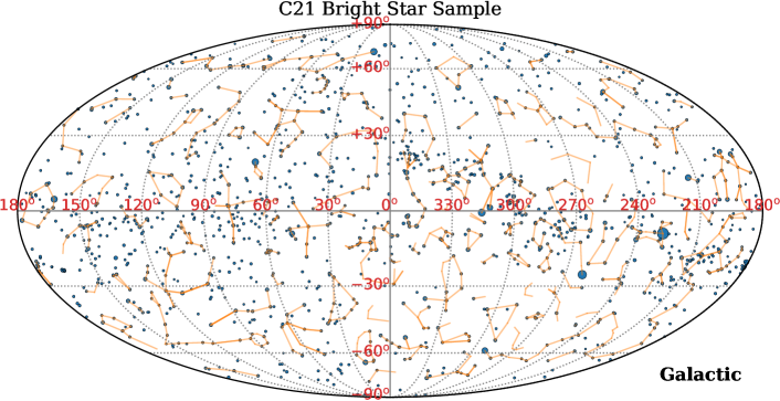
Figure 1: Distribution in the celestial sphere (Galactic coordinates) of the C21 bright star sample, constituted by 1346 stars. Simple constellation shapes (van der Sluys, 2005), displayed with light orange lines, are also shown to facilitate the visual identification of the stars. The size of each star symbol is inversely proportional to its green RGB magnitude, as derived by C21.

Although the C21 catalogue of RGB magnitudes is suitable for calibration purposes, it only contains a small number of stars (on average 1 star for each 30 square degrees, although they tend to concentrate towards the Galactic plane; see Fig. 1). Not only that, this catalogue is constituted by stars brighter than Johnson $V=6.6$ mag, with a magnitude distribution whose 16th, 50th and 84th percentiles are 3.3, 4.4 and 5.0 mag, respectively. This is specially problematic when considering astronomical projects that could seriously benefit from the exponential growth of the number of professional and amateur astronomers equipped with commercial-grade RGB cameras, who can potentially generate a huge amount of useful data in many astronomical fields (see the Introduction section in C21 and references therein).

The aim of this paper is to exploit the superb photometric data provided by the Gaia mission (Gaia Collaboration et al., 2016), through the third intermediate Gaia data release (Gaia Collaboration et al., 2021, Gaia EDR3), to estimate RGB magnitudes from Gaia $G$, $G_{\rm BP}$ and $G_{\rm RP}$ photometric data. For that purpose, we have derived simple transformations between those magnitudes and the synthetic RGB photometry in the sample of bright stars published by C21. In order to avoid confusion between Gaia $G$ magnitudes and the ones corresponding to the green RGB filter, from this point we are using $G^{\rm Gaia}$, $G_{\rm BP}^{\rm Gaia}$ and $G_{\rm RP}^{\rm Gaia}$ to indicate the use of the Gaia magnitudes, and $B^{\rm rgb}$, $G^{\rm rgb}$ and $R^{\rm rgb}$ when referring to the RGB photometric measurements.

Since the C21 star sample is constituted by bright and nearby stars of metallicity slightly undersolar (as shown in Sect. 2.1), we have also employed synthetic Gaia and RGB magnitudes measured in stellar atmosphere models to constrain the systematic uncertainties introduced by the use of the mentioned transformations with stars of different metallicity and also affected by interstellar extinction. In addition, we have applied the fitted transformations to estimate RGB magnitudes for a sample of $\sim 15$ million stars extracted from the sample of Anders et al. (2019). These authors published improved photo-astrometric distances, extinctions and astrophysical parameters for Gaia DR2 stars brighter than $G=18$ mag, using for that purpose the Bayesian tool StarHorse (Queiroz et al., 2018), complementing the Gaia measurements with Pan-STARRS1, 2MASS and AllWISE photometric data. Here we have restricted their stellar sample to minimize the impact of systematic uncertainties, introduced by metallicity variations and interstellar extinction, in the predictions of RGB magnitudes.

Synthetic magnitudes in this work have been determined using the Python package synphot (STScI development Team, 2018), which facilitates the computation of photometric properties from user-defined bandpasses and spectra (see Section 2 of C21 for additional computational details).

The description of the Gaia–RGB calibration is presented in Section 2. Its application to the StarHorse subsample of 15 million stars is described in Section 3, while the final discussion and conclusions are summarized in Section 4. Appendix A describes how to extend the estimation of RGB magnitudes beyond the 15 million star sample, by using ADQL queries to the Gaia catalogue and an auxiliary Python package specially written for that purpose.

2 RGB calibration from Gaia EDR3 photometry

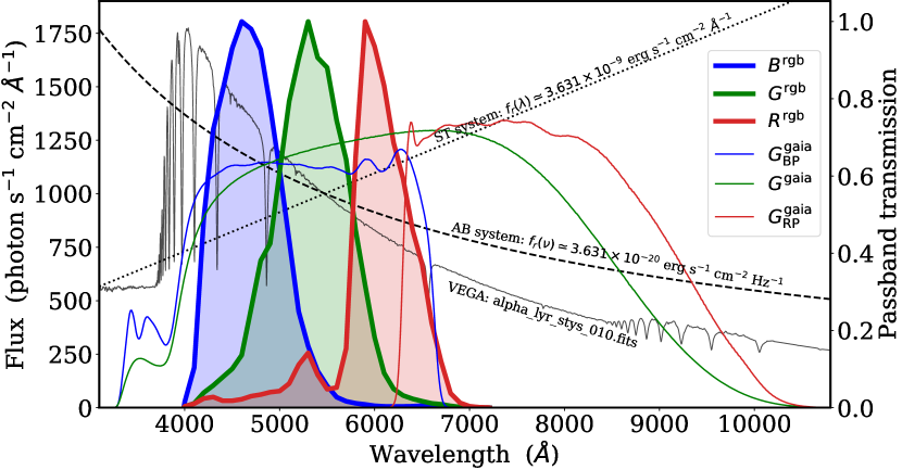
Figure 2: Comparison of the transmissivity of the Gaia EDR3 passbands (thin blue, green and red lines), derived by Riello et al. (2021), with the standard RGB passbands defined in C21 (thick blue, green and red lines encompassing shaded regions). The flux density (in photon s^-1 cm^-2 Å^-1) of the reference spectra used to define magnitudes in the common AB, ST and Vega systems are shown as dashed, dotted and full black lines, respectively.

The RGB sensitivity curves of the standard photometric system defined by C21 are encompassed by the transmissivity of the Gaia EDR3 passbands derived by Riello et al. (2021) (see Fig. 2). In particular, the three RGB transmissivity curves cover a similar wavelength range as $G_{\rm BP}^{\rm Gaia}$, and approximately half of the range spanned by $G^{\rm Gaia}$. The fact that $G_{\rm RP}^{\rm Gaia}$ covers an additional range towards longer wavelengths, makes the colour $G_{\rm BP}^{\rm Gaia}-G_{\rm RP}^{\rm Gaia}$ a good proxy to estimate variations in the spectral energy distribution covered in the visible range. For that reason, it is expected that a good calibration of RGB magnitudes can be derived from the accurate Gaia data. In this section we describe the procedure followed to achieve this task, starting by collecting the Gaia magnitudes available for the C21 bright star sample, creating colour-colour diagrams involving Gaia and RGB magnitudes, and finding a simple mathematical relationship between both magnitude sets.

2.1 Gaia EDR3 data for the C21 bright star sample

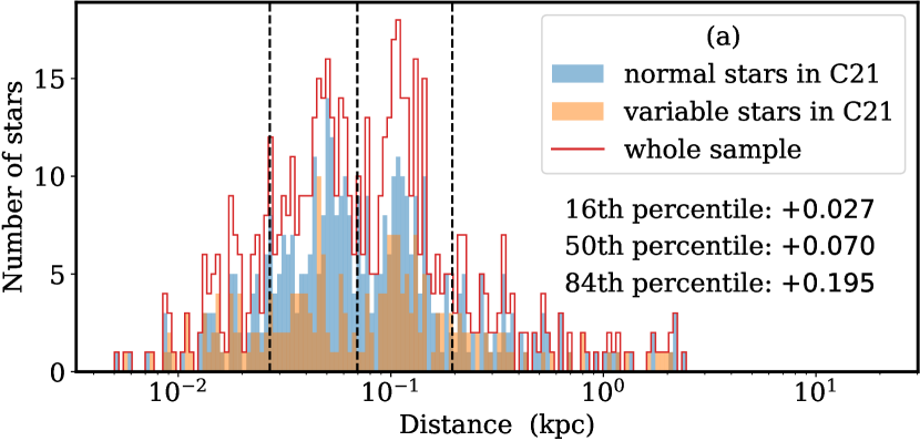
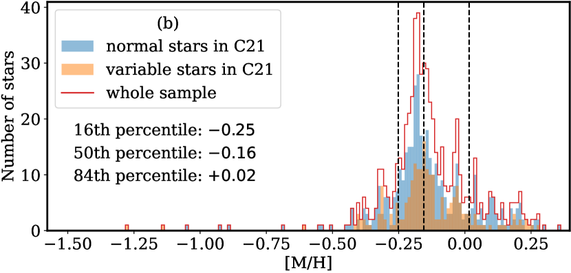
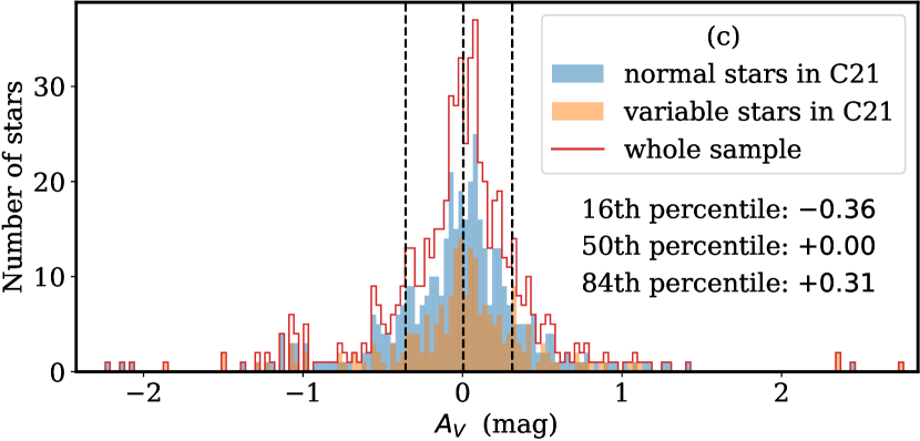
Figure 3: Panels (a)–(c): histograms displaying the distributions in distance [panel (a)], metallicity [panel (b)] and $A_{V}$ extinction [panel (c)] for the C21 bright star subsample in common with Anders et al. (2019). These three parameters are the ones derived by these authors using StarHorse. Although initially 785 stars had parameter estimates, 172 stars were discarded by imposing the quality flag SH_OUTFLAG=’00000’, which guarantees the statistical reliability of the StarHorse determinations. The histograms have been computed separately for the non-variable (in blue) and variable (orange) stars, with the red line delineating the coadded histogram. The three vertical dashed lines indicate the 16th, 50th and 84th percentiles (from left to right, respectively) of the whole displayed sample, whose values are provided under the plot legend. Panel (d): histogram displaying the 5th, 50th and 95th percentile of the posterior probability distribution for the StarHorse $A_{V}$ estimates. Note that the 50th percentile histogram is the same displayed in panel (c) for the whole sample with reliable parameters, whereas the 95th percentile is greater than zero for all the stars with SH_OUTFLAG=’00000’. This indicates that the negative $A_{V}$ values correspond to stars whose Bayesian posterior probability distribution is not statistically incompatible with a null extinction.

As the first step for this work, we retrieved the $G^{\rm Gaia}$, $G_{\rm BP}^{\rm Gaia}$ and $G_{\rm RP}^{\rm Gaia}$ magnitudes for the bright star sample of C21, provided by the Gaia EDR3 (Gaia Collaboration et al., 2021) Archive at the European Space Agency. This process was carried out in the following way: the Gaia DR2 identifier of each star was initially obtained through the Simbad database, starting from the initial HR number of the star in the Bright Star Catalogue (Hoffleit, 1964). Since it is not guaranteed that the same astronomical source will always have the same source identifier in the different Gaia Data Releases, for each source_id in DR2 we searched for proximal source(s) in the auxiliary table gaiaedr3.dr2_neighbourhood, keeping the most likely crossmatch taking into account the parameters angular_distance and magnitude_difference when more that one possible counterpart appeared. It is important to note that not all the bright stars in the C21 sample appear in the Gaia database because of its level of incompleteness at the bright end (Gaia Collaboration et al., 2021). In addition, and having in mind that our main goal is to derive a photometric transformation, we imposed the signal-to-noise ratio for the flux measured by Gaia in each passband to be high enough to guarantee a maximum uncertainty of 0.01 mag for both $G^{\rm Gaia}$ magnitudes and the $G_{\rm BP}^{\rm Gaia}\!-\!G_{\rm RP}^{\rm Gaia}$ colours. At the end of this process, the initial sample of 1346 bright stars was finally reduced to a subsample of 888 objects, 320 of them flagged as variable stars in Simbad, and 568 with no indication of variability. The histograms displayed in Fig. 3 confirm that the bulk of this bright star C21 subsample is dominated by nearby stars, with metallicity slightly undersolar and scarcely affected by interstellar extinction. Although the large negative extinction estimates displayed in Fig. 3(c) may seem alarming, it is important to realize that they simply correspond to the median values of the $A_{V}$ Bayesian posterior probability distribution derived by Anders et al. (2019) for each star, and thus, a too simplistic reduction of whole probability distributions into single numbers. The 5th and 95th percentile $A_{V}$ values displayed in Fig. 3(d) illustrate that the credible intervals for those stars are compatible with $A_{V}=0$.

2.2 Colour–colour diagram relating RGB and Gaia

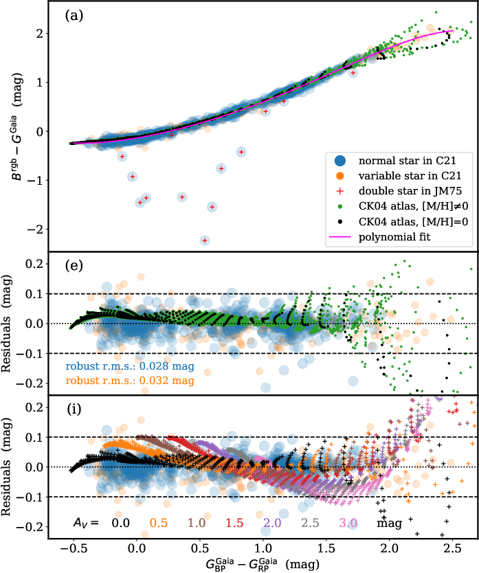
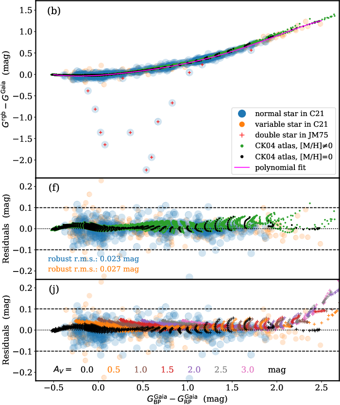
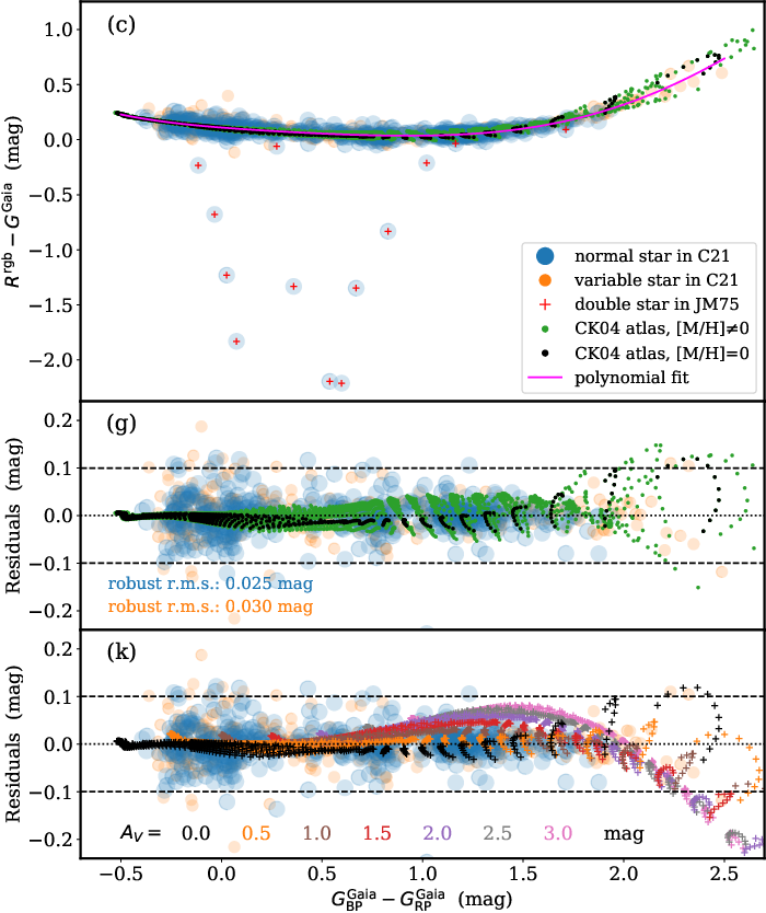
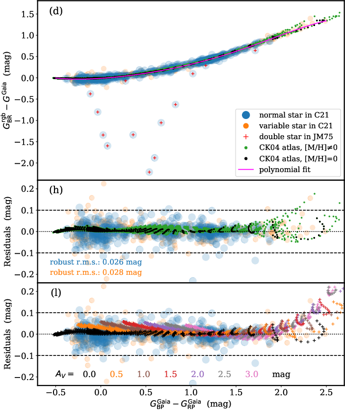
Figure 4: Panels (a), (b), (c) and (d): colour-colour diagrams representing the differences between each RGB magnitude (and $G^{\rm rgb}_{\rm BR}$) with $G^{\rm Gaia}$ as a function of the Gaia colour  $G_{\rm BP}^{\rm Gaia}\!-\!G_{\rm RP}^{\rm Gaia}$. The bright star sample from C21 is plotted with filled blue (non-variable stars) and orange (stars flagged as variable in Simbad) circles. Clear outliers, overplotted with a small red cross, correspond to double stars in Johnson & Mitchell (1975) (JM75, see text). The predictions of CK04 models are also shown with small black (solar metallicity) and green (non-solar metallicity) circles. The calibrations, robust fits to 5-degree polynomials, are shown as magenta lines, with the corresponding residuals shown (twice) in the underneath panels. Panels (e), (f), (g) and (h): the r.m.s. of the residuals is provided separately for the non-variable (blue) and variable (orange) stars. The horizontal dashed lines encompass the $\pm 0.1$ mag interval. Panels (i), (j), (k) and (l): the coloured crosses indicate the impact of interstellar reddening, as parametrized by the indicated $A_{V}$ values, for CK04 models of solar metallicity (non-solar predictions have not been used in this case to avoid cluttering).

We represent in the top panels of Fig. 4 the colour–colour diagrams built using the difference between each RGB magnitude (from the C21 catalogue) and $G^{\rm Gaia}$, as a function of the Gaia colour $G_{\rm BP}^{\rm Gaia}\!-\!G_{\rm RP}^{\rm Gaia}$. We have also included in this comparison an estimate of the magnitude in the green RGB filter computed simply as the arithmetic mean of the two magnitudes in the neighbouring filters, i.e.,

$$G^{\rm rgb}_{\rm BR}=\frac{B^{\rm rgb}+R^{\rm rgb}}{2}.$$ (1)

The definition of this additional magnitude can be particularly useful for observations performed with cameras equipped with Bayer-like colour filter systems, in which an array of luminance- and chrominance-sensitivity elements (the green pixels on the one hand, and the blue and red pixels, on the other) are superposed in registration with an imaging array. Since the spatial sampling of each pixel is different, the computation of an averaged (blue+red) magnitude can facilitate the estimation of an independent green magnitude which, in addition, can help to perform image interpolations through the comparison of the demosaiced RGB channels.

Non-variable stars in the colour-colour diagrams shown in Fig. 4 are represented with big blue filled circles, whereas variable objects are plotted with smaller orange filled circles. It is clear that the subsample of C21 bright stars with Gaia data exhibits well-defined sequences in these diagrams. A few objects, outliers in the four panels and marked with an additional red cross, correspond to stars flagged as double in the initial photometric measurements by Johnson & Mitchell (1975) (see also Table 3 in C21) and were not used in the subsequent work. We have also overplotted the expected location of synthetic colour estimates computed from the stellar atmosphere models by Castelli & Kurucz (2003, hereafter CK04), which are precomputed for abundances ${\rm[M/H]}\!=\!-2.5$, $-2.0$, $-1.5$, $-1.0$, $-0.5$, $0.0$, $+0.2$ and $+0.05$, effective temperatures ranging from 3500 to 50000 K, and $\log g$ (surface stellar gravity, with $g$ in cm s^-2) from 0.0 to 5.0 dex. Note that these are the same models employed by C21 to derive their RGB photometric database. In particular, we have used two different symbol colours to represent the predictions for solar metallicity stars (small black filled circles) and for non-solar metallicity objects (small green filled circles). It is important to highlight here that the RGB photometric system is defined in the absolute (AB) scale, whereas the Gaia magnitudes are provided in the Vega system. The latter have been computed for the synthetic magnitudes of the stellar models using the Vega spectrum alpha_lyr_stys_010.fits, available at the CALSPEC database (Bohlin et al., 2014).

2.3 The Gaia-RGB calibration

Table 1: Coefficients of the polynomials $f_{B}$, $f_{G}$, $f_{R}$ and $f_{G_{\rm BR}}$ defined in Eqs. (2)–(5), and corresponding to the fits displayed with magenta lines in panels (a), (b), (c) and (d) of Fig. 4. Each polynomial must be evaluated as   $f_{X}=\sum_{i=0}^{5}a_{i}\,(G_{\rm BP}^{\rm Gaia}\!-\!G_{\rm RP}^{\rm Gaia})^{i}$, with $X=B,\,G,\,R$ and $G_{\rm BR}$.

Coef.	$f_{B}$	$f_{G}$	$f_{R}$	$f_{G_{\rm BR}}$
$a_{0}$	$-0.13748689$	$-0.02330159$	$+0.10979647$	$-0.01252185$
$a_{1}$	$+0.44265552$	$+0.12884074$	$-0.14579334$	$+0.13983574$
$a_{2}$	$+0.37878846$	$+0.22149167$	$+0.10747392$	$+0.23688188$
$a_{3}$	$-0.14923841$	$-0.14550480$	$-0.10635920$	$-0.10175532$
$a_{4}$	$+0.09172474$	$+0.10635149$	$+0.08494556$	$+0.07401939$
$a_{5}$	$-0.02594726$	$-0.02363990$	$-0.01368962$	$-0.01821150$

The sequences displayed in the top panels of Fig. 4 have been iteratively fitted (rejecting outliers using a sigma-clipping algorithm) to the previously described subsample of 888 bright stars, using fifth-order polynomials. Since the stars included in this subsample flagged as variable objects already passed the filtering process described in C21 when comparing synthetic Johnson $B$ and $V$ magnitudes with tabulated measurements in the Simbad database, and considering that they do not show a different behaviour to that exhibited by non-variable stars, we kept them in the initial set to be fitted, knowing that the sigma-clipping algorithm would get rid off the deviant cases. With the aim of constraining the fits at the extremes of the $G_{\rm BP}^{\rm Gaia}\!-\!G_{\rm RP}^{\rm Gaia}$ colour interval, the fitted data were complemented by including the predictions of the CK04 models of solar metallicity for $-0.5<G_{\rm BP}^{\rm Gaia}\!-\!G_{\rm RP}^{\rm Gaia}<-0.4$ mag and for $2.0<G_{\rm BP}^{\rm Gaia}\!-\!G_{\rm RP}^{\rm Gaia}<2.5$ mag (no additional model data were employed except for those two small colour ranges at the borders). The fitted relationships are displayed in the top panels of Fig. 4 with a continuous magenta line, and the resulting residuals are plotted (twice) in the central and bottom panels. These polynomial fits provide the sought transformation that allows estimating RGB magnitudes from the Gaia magnitudes using

$$B^{\rm rgb}= \mbox{}\;\;G^{\rm Gaia}+f_{B}(G_{\rm BP}^{\rm Gaia}\!-\!G_{\rm RP}^{\rm Gaia}),$$ (2)

$$G^{\rm rgb}= \mbox{}\;\;G^{\rm Gaia}+f_{G}(G_{\rm BP}^{\rm Gaia}\!-\!G_{\rm RP}^{\rm Gaia}),$$ (3)

$$R^{\rm rgb}= \mbox{}\;\;G^{\rm Gaia}+f_{R}(G_{\rm BP}^{\rm Gaia}\!-\!G_{\rm RP}^{\rm Gaia}),$$ (4)

$$G^{\rm rgb}_{\rm BR}= \mbox{}\;\;G^{\rm Gaia}+f_{G_{\rm BR}}(G_{\rm BP}^{\rm Gaia}\!-\!G_{\rm RP}^{\rm Gaia}),$$ (5)

where $f_{B}$, $f_{G}$, $f_{R}$ and $f_{G_{\rm BR}}$ are the fifth-order polynomials with independent variable $G_{\rm BP}^{\rm Gaia}\!-\!G_{\rm RP}^{\rm Gaia}$, whose coefficients are given in Table 1.

The residuals are displayed in the central panels of Fig. 4, using the same symbols employed in the top panels. The robust standard deviation of these residuals is also provided within each panel, computed separately for the 568 non-variable stars (blue colour) and the 320 variable stars (orange colour), being the latter slightly larger in the four panels. In all cases, the $\pm 3\sigma_{\rm robust}$ dispersion is constrained within the $\pm 0.1$ mag interval (displayed with the horizontal dashed lines). The same panels also display the residuals corresponding to the synthetic magnitudes derived from the CK04 models: the predictions for solar metallicity stars (small black filled circles) are well reproduced by the previous fitted relationships, except for the reddest stars, where the dispersion increases. The models with metallicity different from solar (small green filled circles) exhibit a wider scatter. It is interesting to note that the model predictions interpolated for ${\rm[M/H]}\!=\!-0.16$, the median value in Fig. 3(b), are not very different from those for solar metallicity. In particular, the comparison between all the models predictions leads to

$$\Delta(G_{\rm BP}^{\rm Gaia}-G_{\rm RP}^{\rm Gaia}) =0.004\pm 0.014\;{\rm mag},$$ (6)

$$\Delta(B^{\rm rgb}-G^{\rm Gaia}) =0.004\pm 0.008\;{\rm mag},$$ (7)

$$\Delta(G^{\rm rgb}-G^{\rm Gaia}) =0.002\pm 0.009\;{\rm mag},$$ (8)

$$\Delta(R^{\rm rgb}-G^{\rm Gaia}) =0.002\pm 0.009\;{\rm mag,\;and}$$ (9)

$$\Delta(G_{\rm BR}^{\rm rgb}-G^{\rm Gaia}) =0.002\pm 0.010\;{\rm mag},$$ (10)

where each $\Delta$ value corresponds to the mean (and associated standard deviation) colour difference between the ${\rm[M/H]}\!=\!0.0$ and the ${\rm[M/H]}\!=\!-0.16$ predictions. Interestingly, all the models fit within the $\pm 0.1$ mag interval for $G^{\rm rgb}$ and $G^{\rm rgb}_{\rm BR}$, whereas the same is true for $B^{\rm rgb}$ and $R^{\rm rgb}$ when restricting to the $-0.5<G_{\rm BP}^{\rm Gaia}\!-\!G_{\rm RP}^{\rm Gaia}<2.0$ mag range.

The residuals of the fitted data are displayed again in the bottom panels of Fig. 4, but in this case the overplotted model predictions represent the residuals of the CK04 models after reddening them employing the extinction law of Cardelli et al. (1989) (updated by O’Donnell, 1994), with a relative extinction parameter $R_{V}=3.1$ and variable extinctions $A_{V}$ ranging from 0.5 to 3.0 mag (crosses of different colours). Interestingly, the extinction reddens the data basically along the sequences already displayed in the top panels, and therefore the residuals in the bottom panels remain constrained within the $\pm 0.1$ mag interval. The effect is larger in $B^{\rm rgb}$ and $R^{\rm rgb}$ than in $G^{\rm rgb}$ and $G^{\rm rgb}_{\rm BR}$, with a systematic variation as a function of the $G_{\rm BP}^{\rm Gaia}\!-\!G_{\rm RP}^{\rm Gaia}$ colour.

3 Predicting RGB magnitudes for 15 million stars

Table 2: First ten rows of the table with the 14 854 959 stars with RGB predictions. The full table is electronically available at http://guaix.fis.ucm.es/~ncl/rgbphot/gaia. Column description: (1) source identifier in the Gaia EDR3; (2)–(3) star coordinates (J2000), as provided by the EDR3; (4)–(7) RGB magnitudes computed using the transformations given by Eqs. (2)–(5); (8)–(10) Gaia magnitudes in the EDR3; (11)–(13) 50th percentile (median) of the interstellar extinction $A_{V}$ (mag), [M/H] and distance (kpc), computed by Anders et al. (2019) using StarHorse.

(1)	(2)	(3)	(4)	(5)	(6)	(7)	(8)	(9)	(10)	(11)	(12)	(13)
EDR3 source_id	RA (°)	DEC (°)	$B^{\rm rgb}$	$G^{\rm rgb}$	$R^{\rm rgb}$	$G^{\rm rgb}_{\rm BR}$	$G^{\rm Gaia}$	$G^{\rm Gaia}_{\rm BP}$	$G^{\rm Gaia}_{\rm RP}$	av50	met50	dist50
2875513285079465984	0.000095821	$+34.987630914$	17.03	16.46	16.06	16.55	15.9741	16.6310	15.2054	$+0.120$	$-0.188$	$+0.612$
393915403758148352	0.000114124	$+50.277031947$	18.58	18.14	17.84	18.21	17.7949	18.3144	17.1386	$+0.158$	$-0.005$	$+1.818$
4702040864637495296	0.000141937	$-71.574692515$	18.15	17.76	17.49	17.82	17.4528	17.9223	16.8279	$-0.239$	$-0.111$	$+1.720$
384492417301984256	0.000168528	$+43.261207984$	16.71	16.43	16.25	16.48	16.2111	16.5778	15.6839	$+0.122$	$+0.027$	$+1.952$
2746773530168227328	0.000178628	$+08.371651685$	12.85	12.40	12.09	12.47	12.0394	12.5638	11.3628	$+0.197$	$-0.048$	$+0.143$
2855280484422222336	0.000262145	$+29.896074086$	18.08	17.45	16.99	17.54	16.8718	17.6054	16.0451	$-0.129$	$-0.019$	$+0.771$
2875090969535427072	0.000301072	$+33.520870876$	16.81	16.53	16.34	16.57	16.3041	16.6743	15.7705	$+0.209$	$-0.224$	$+1.637$
2443095153084654080	0.000434825	$-05.494409354$	09.63	09.21	08.92	09.27	08.8720	09.3678	08.2151	$+0.139$	$-0.316$	$+0.518$
4923847544332011520	0.000435338	$-54.929637980$	14.29	14.10	13.99	14.14	13.9466	14.2257	13.5046	$+0.065$	$-0.160$	$+0.920$
2745049530295263232	0.000589823	$+05.380517265$	13.98	13.43	13.03	13.51	12.9555	13.5889	12.1934	$+0.038$	$-0.235$	$+0.149$

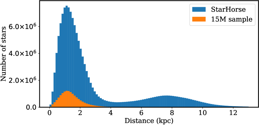
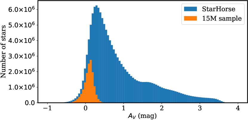
Figure 5: Histograms displaying the distributions in distance (top panel), metallicity (middle panel) and $A_{V}$ extinction (bottom panel) for the 136 606 075 stars composing the StarHorse sample restricted to SH_GAIAFLAG=’000’ and SH_OUTFLAG=’00000’ (blue colour), and for the 14 854 959 stars constituting the filtered 15M star sample (orange colour).

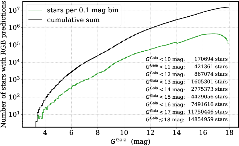
Figure 6: Variation of the number of stars with RGB magnitude predictions as a function of $G^{\rm Gaia}$. The green curve shows the histogram in bins of 0.1 mag, whereas the black line displays the cumulative sum. The inset tabulates the cumulative sum down to some particular $G^{\rm Gaia}$ values.

We have applied the RGB calibration derived in the previous section to the StarHorse star sample of Anders et al. (2019). The data was retrieved from the Gaia archive hosted by the Leibniz-Institute for Astrophysics Potsdam. With the aim of using the star subsample with the most reliable distance, extinction and astrophysical parameter determinations, we restricted the initial list to 136 606 075 stars flagged with SH_GAIAFLAG=’000’ (indicating good astrometric and photometric quality of the Gaia DR2 data) and SH_OUTFLAG=’00000’ (associated to stars with reliable StarHorse output parameters). It is worth noting that by adopting these values of SH_GAIAFLAG and SH_OUTFLAG we excluded from the beginning stars identified as variable in Gaia DR2 (entry phot_variable_flag in the database), as well as objects with significantly negative extinctions or with large $A_{V}$ uncertainties. From this initial collection, 13 756 448 stars were removed due to multiple potential candidates in the crossmatch between DR2 and EDR3 (parameter dup_max_number greater than one). Then, we selected stars with extinction estimates compatible with zero within the 16th and 84th $A_{V}$ percentiles computed by Anders et al. (2019) when deriving the astrophysical parameters of the StarHorse sample, which restricted the sample to 20 477 474 stars. At this point, the cut $-0.5<G_{\rm BP}^{\rm Gaia}\!-\!G_{\rm RP}^{\rm Gaia}<2.0$ mag was imposed to match the valid colour interval where Eqs. (2)–(5) can be employed, leading to a collection of 19 567 621 objects. Finally, we also constrained the estimated metallicity for each star to be compatible with the median value ${\rm[M/H]}=-0.16$ exhibited by the C21 calibrating sample (middle panel in Fig. 3) within the 16th and 84th [M/H] percentile interval derived by Anders et al. (2019). This last step led to the final set of 14 854 959 stars (hereafter the 15M star sample) for which we have estimated the RGB magnitudes. The predicted values are given in Table 2.

The histograms displayed in Fig. 5 compare the distributions in distance (top panel), metallicity [M/H] (middle panel) and interstellar extinction $A_{V}$ (bottom panel) of the 15M star subsample (orange colour) with those exhibited by the initial $\sim 136$ million stars corresponding to the StarHorse sample (blue colour). Although the strong constraint introduced when selecting stars with extinction estimates compatible with zero does not introduce a systematic bias in the metallicity distribution, it imposes a clear restriction in the distance coverage: most of the 15M star sample is composed of stars closer than 3 kpc to the Sun.

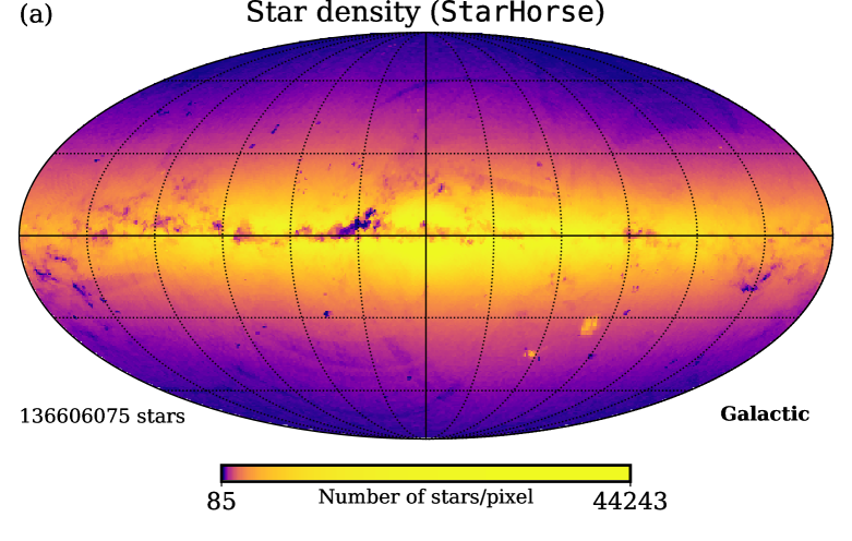
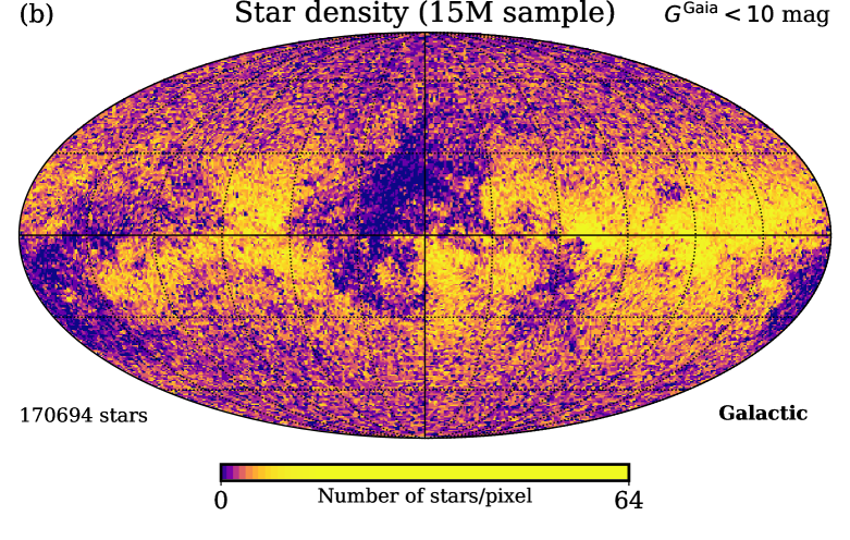
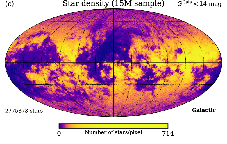
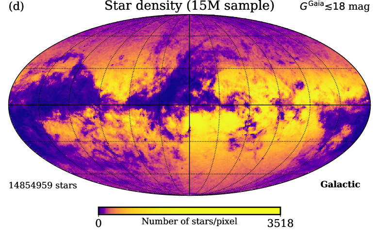
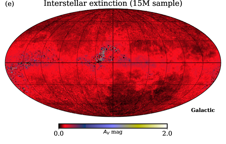
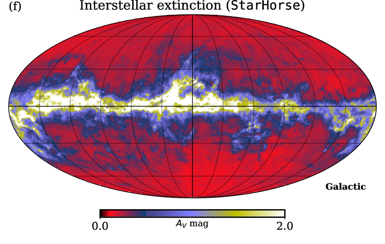
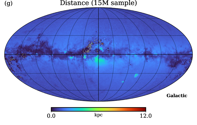
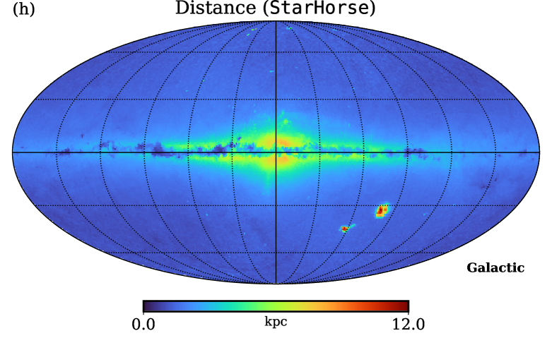
Figure 7: Panel (a): star density map, in Galactic coordinates, corresponding to the 136 606 075 stars in the StarHorse sample of Anders et al. (2019) flagged with SH_GAIAFLAG=’000’ and SH_OUTFLAG=’00000’. Panels (b) (c) and (d): star density maps corresponding to the stars with estimated RGB magnitudes (i.e., those in the 15M star sample) for different limiting $G^{\rm Gaia}$ magnitudes: 10, 14 and 18 mag for panels (b), (c) and (d), respectively. These maps have been created using HEALPix of level 6 (providing a pixel size of 0.84 square degrees), and are colour coded depending on the number of stars within the pixel. Panels (e) and (f): extinction maps representing the mean $A_{V}$ values within each HEALPix of level 6, exhibited by the 15M sample, panel (e), and the 136 606 075 stars in the StarHorse sample, panel (f). Panels (g) and (h): mean distance (kpc) within each HEALPix of level 6 for the stars in the 15M sample, panel (g), and the mentioned StarHorse sample, panel (h). The coordinate origin and grid in all the panels are the same employed in Fig. 1.

The number of stars in the 15M sample, as a function of the $G^{\rm Gaia}$ magnitude, is shown in Fig. 6 (green line). As expected, this number increases when moving to fainter objects. The cumulative number of stars down to a given magnitude is also displayed (black line), with the total number of stars down to some particular $G^{\rm gaia}$ values listed within the figure.

The global distribution in the celestial sphere of the 136 606 075 stars in the StarHorse sample of Anders et al. (2019) flagged with SH_GAIAFLAG=’000’ and SH_OUTFLAG=’00000’ is shown in panel (a) of Fig. 7 (using Galactic coordinates, with HEALPix of level 6). It is clear that most of the stars concentrate towards the Galactic plane. For comparison, panels (b), (c) and (d) of Fig. 7 show the same map for the 15M star sample restricted to different limiting $G^{\rm gaia}$ magnitudes. In addition, panels (e) and (f), on one hand, and panels (g) and (h), on the other, compare, respectively, the mean extinction $A_{V}$ (mag) and distance (kpc) exhibited by the 15M sample and the initial StarHorse star collection. These maps show that the stars in the 15M sample are unevenly spread because high-extinction regions, clearly seen in panel (f), have been purposely avoided, being the $A_{V}$ values of the 15M star sample, panel (e), quite small. This behaviour is consistent with the distance maps, which confirm that the 15M sample, panel (g), is constituted by nearby stars, as already shown in the histogram of Fig. 5(a), specially at low Galactic latitudes.

4 Final discussion and conclusions

The work presented in the previous sections has shown that it is possible to derive simple mathematical transformations between Gaia EDR3 photometric data and RGB magnitudes, and to employ them to substantially extend, both in quantity and magnitude coverage, the number of stars in the celestial sphere with RGB magnitude estimates. The comparison with measurements performed using stellar atmosphere models (covering [M/H] from $-2.5$ to $+0.5$, effective temperatures from 3500 to 50000 K, and $\log g$ from 0.0 to 5.0 dex) has revealed that Eqs. (2)–(5) are expected to provide RGB estimates within a $\pm 0.1$ mag uncertainty when imposing the colour cut $-0.5<G_{\rm BP}^{\rm Gaia}\!-\!G_{\rm RP}^{\rm Gaia}<2.0$ mag. The predicted magnitudes remain within the $\pm 0.1$ mag interval even when considering interstellar extinctions in the range $A_{V}\in[0.0,3.0]$ mag, although there are some systematic deviations depending on the $G_{\rm BP}^{\rm Gaia}\!-\!G_{\rm RP}^{\rm Gaia}$ colour, being $G^{\rm rgb}$ and $G_{\rm BR}^{\rm rgb}$ more robust to this effect than $B^{\rm rgb}$ and $R^{\rm rgb}$. For that reason, we have restricted the star sample to nearby objects for which the interstellar extinction estimate derived by Anders et al. (2019) was statistically compatible with zero.

The new catalogue, encompassing $\sim 15$ million stars, should smooth the way for:

• The use of the standard RGB photometric system proposed by C21: the homogenization of RGB measurements, derived from data obtained with a potentially very large number of different cameras, will become essential. This is a critical aspect that can hardly be overestimated.

• The proper calibration of commercial-grade RGB cameras: this task will be facilitated by considering the wide magnitude range exhibited by the 15M star sample, leaving ample room for the use of RGB imaging instruments with different field of views, as well as their exploitation in scientific projects requiring distinct exposure times.

• The calibration of observations carried out in any region of the sky, even at high Galactic latitudes. Note, however, that the distribution in the celestial sphere is inhomogeneous and depends on the interstellar extinction in the direction of observation, being the total number of available calibrated stars unavoidably tied to the adopted limiting magnitude.

• The correction of the measurements for atmospheric extinction: this data reduction step is particularly important in wide-field exposures, where stars at different airmasses are simultaneously observed.

It is important to highlight that the RGB magnitude predictions computed for the 15M star sample should not be considered to be extremely accurate on a star by star basis. In particular, although stars detected as variables in DR2 have been removed, it is likely that variable sources are still hidden in the selected sample. In any case, the large number of calibrating stars available should facilitate the computation of statistical averages that allow the rejection of potential outliers, guaranteeing adequate calibrations.

Although in this work we have restricted the RGB estimates to a subsample of the stars published by Anders et al. (2019) with good photo-astrometric distances, extinctions and astrophysical parameters, it is possible to apply the derived calibrations to many more Gaia EDR3 stars for which these parameters are not even available. In principle, this should only be employed for stars with high Galactic latitude in order to minimize systematic errors introduced by interstellar extinction (although there are regions with low galactic latitude and low extinction), and within the colour interval $-0.5<G_{\rm BP}^{\rm Gaia}\!-\!G_{\rm RP}^{\rm Gaia}<2.0$ mag. In this regard, it is interesting to note that $\sim 82$ per cent of the 304 602 695 stars available in Gaia EDR3 with $G^{\rm Gaia}\leq 18$ mag (251 118 359 stars) verify the last colour cut. This means that, down to a given limiting magnitude, the total number of observable stars is expected to be much larger than the number of stars belonging to the 15M star sample. The initial calibration obtained by employing the predicted RGB magnitudes presented here, using only a subsample of the observed stars, can be applied, in a second iteration, to the remaining stars verifying the appropriate colour cut. The inclusion of additional stars (after removing outliers) should facilitate the computation of a more reliable calibration. In addition, the relative robustness of $G^{\rm rgb}$ and $G_{\rm BR}^{\rm rgb}$ to moderate amounts of interstellar extinction, should even allow the use of observations performed in regions closer to the Galactic plane (although this should always be double-checked through comparison with calibrations performed at higher Galactic latitudes). With the aim of helping on the use (and extension) of the 15M star sample, in Appendix A we illustrate how to estimate RGB magnitudes for all the Gaia EDR3 stars within a particular cone search.

The synthetic RGB photometry presented here fills an important gap that can help to provide a firm ground for accurate camera calibrations and the systematic exploitation of RGB photometry.

Data Availability

The work in this paper has made use of Gaia DR2 and EDR3, provided by the European Space Agency, the StarHorse database hosted by the Leibniz-Institute for Astrophysics Potsdam, the Stellar Atmopshere Models of Castelli & Kurucz (2003), as provided by the STScI web page, the Bright Star Catalogue (Hoffleit, 1964, available online), and the catalogue of synthethic RGB magnitudes published by Cardiel et al. (2021).

All the results of this paper, together with future additional material, is available online at http://guaix.fis.ucm.es/~ncl/rgbphot/gaia, and will be also available through VizieR.

Appendix A Estimation of RGB magnitudes beyond the 15 million star sample

We illustrate in this appendix how to estimate RGB magnitudes for all the Gaia EDR3 stars within an arbitrary cone search in the celestial sphere. Their use in any calibration procedure should always be accompanied by the observation of reference stars belonging to the 15M star sample.

It is important to remember that Gaia has a bright limit around $G^{\rm Gaia}\sim 3$ mag, and thus, bright stars will be missing.

A.1 Use of an ADQL query

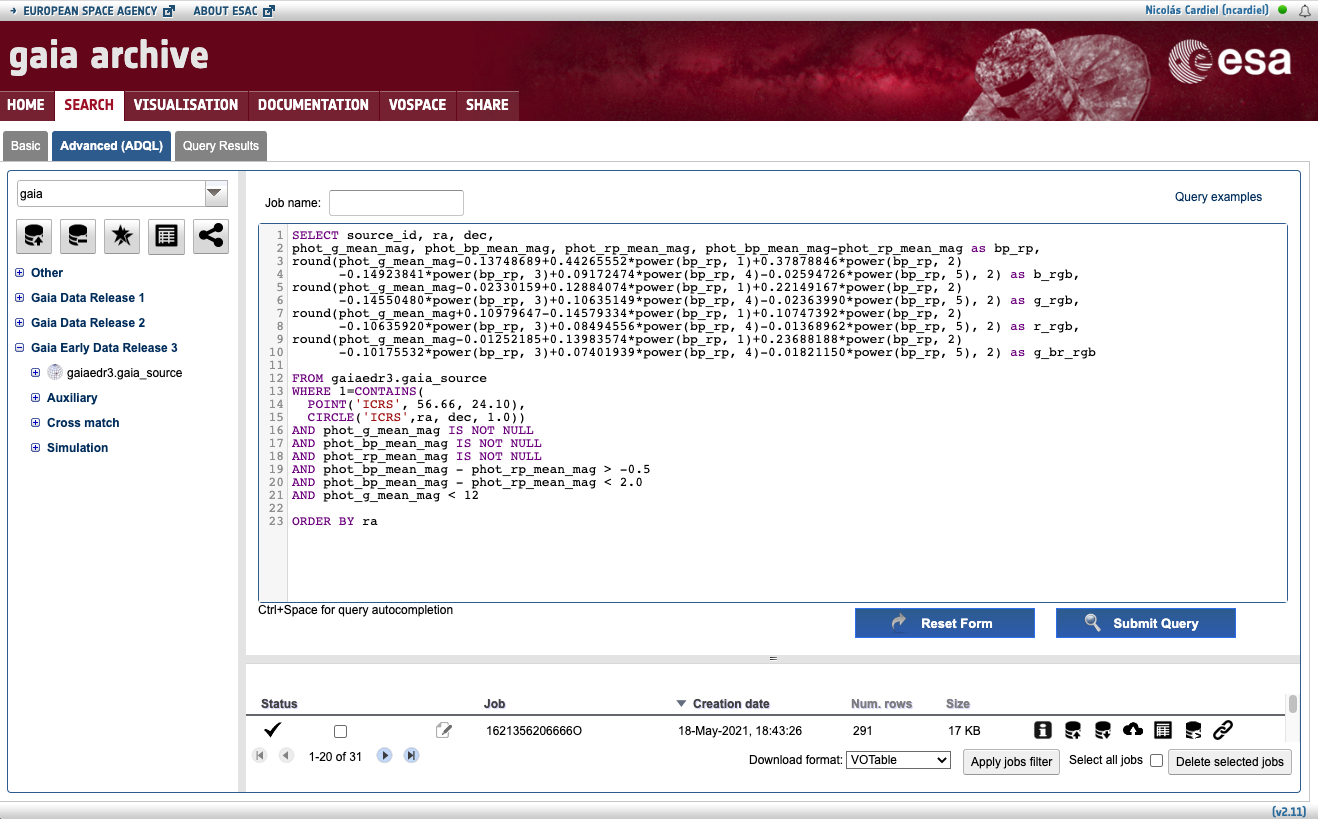
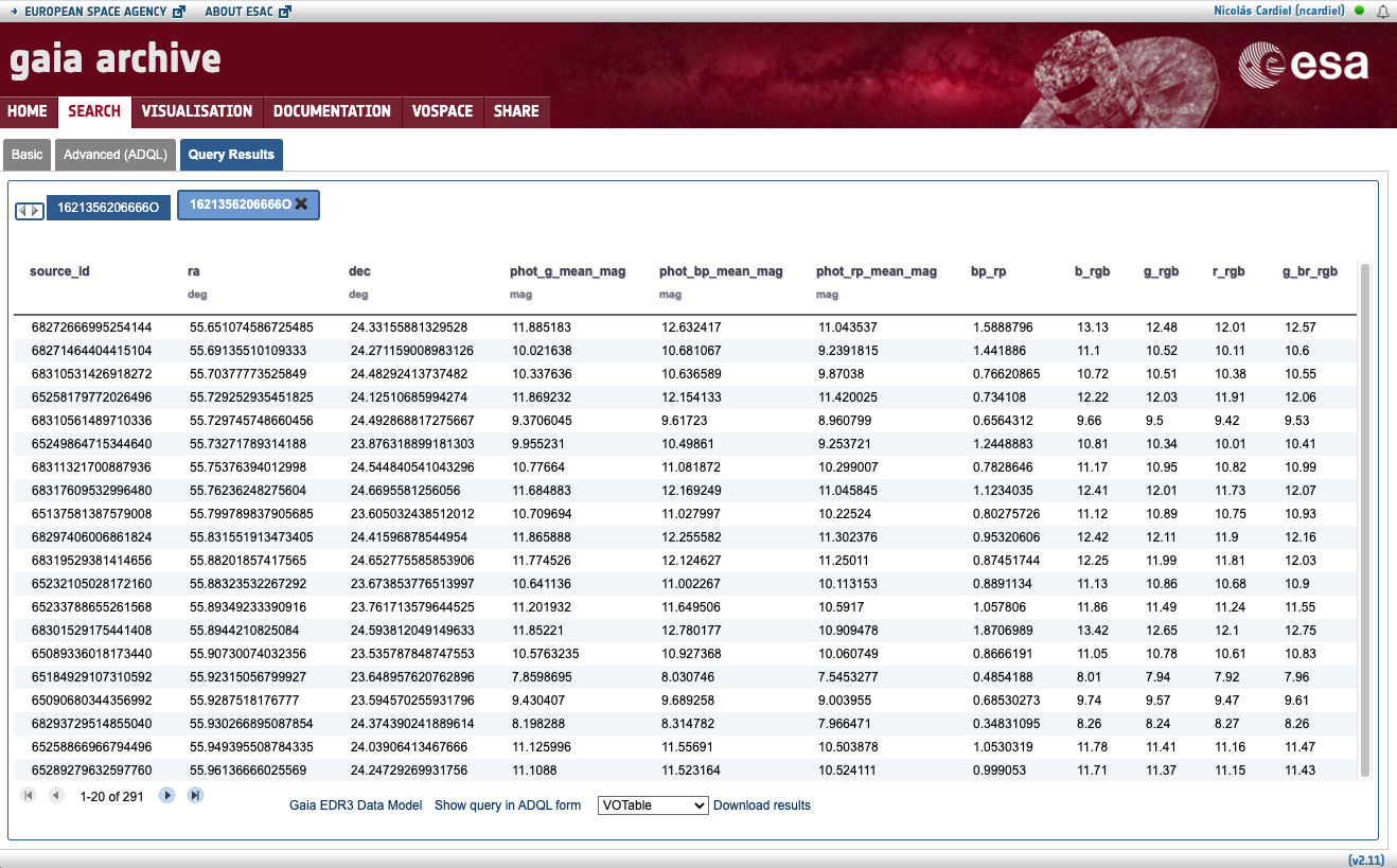
Figure 8: Screenshots of the results of using the ADQL query described in Sect. A.1 in the European Agency Portal of the Gaia EDR3 database. Top panel: interface for advanced queries. The cone search is centrered at RA=56.66°, DEC=24.10° (line number 14 of the displayed query), with a search radius of 1° (line 15), and a limiting $G^{\rm Gaia}$ magnitude of 12 mag (line 21). Bottom panel: table with results. A total of 291 stars match the selection criteria (only the first 20 are displayed), with the RGB magnitude estimates $B^{\rm rgb}$, $G^{\rm rgb}$, $R^{\rm rgb}$ and $G_{\rm BR}^{\rm rgb}$ listed in the last four columns, respectively.

A direct way to retrieve RGB magnitudes is to employ an ADQL (Astronomical Data Query Language; see e.g. Osuna et al., 2008) query to access the Gaia EDR3 database. This language allows to evaluate mathematical expressions on the relevant parameters. For illustration, a simple cone search of Gaia EDR3 stars brighter than $G^{\rm Gaia}\!=\!12$ mag, within a circular region of radius 1°, with centre at RA=56.66°and DEC=24.10° (corresponding to the Pleiades star cluster), imposing the colour selection $-0.5<G_{\rm BP}^{\rm Gaia}\!-\!G_{\rm RP}^{\rm Gaia}<2.0$ mag, and using the polynomial functions given Eqs. (2)–(5) to estimate the RGB magnitudes, can be performed employing:

SELECT source_id, ra, dec,
phot_g_mean_mag, phot_bp_mean_mag, phot_rp_mean_mag,
phot_bp_mean_mag-phot_rp_mean_mag as bp_rp,
round(phot_g_mean_mag
      -0.13748689
      +0.44265552*power(bp_rp, 1)
      +0.37878846*power(bp_rp, 2)
      -0.14923841*power(bp_rp, 3)
      +0.09172474*power(bp_rp, 4)
      -0.02594726*power(bp_rp, 5), 2) as b_rgb,
round(phot_g_mean_mag
      -0.02330159
      +0.12884074*power(bp_rp, 1)
      +0.22149167*power(bp_rp, 2)
      -0.14550480*power(bp_rp, 3)
      +0.10635149*power(bp_rp, 4)
      -0.02363990*power(bp_rp, 5), 2) as g_rgb,
round(phot_g_mean_mag
      +0.10979647
      -0.14579334*power(bp_rp, 1)
      +0.10747392*power(bp_rp, 2)
      -0.10635920*power(bp_rp, 3)
      +0.08494556*power(bp_rp, 4)
      -0.01368962*power(bp_rp, 5), 2) as r_rgb,
round(phot_g_mean_mag
      -0.01252185
      +0.13983574*power(bp_rp, 1)
      +0.23688188*power(bp_rp, 2)
      -0.10175532*power(bp_rp, 3)
      +0.07401939*power(bp_rp, 4)
      -0.01821150*power(bp_rp, 5), 2) as g_br_rgb

FROM gaiaedr3.gaia_source
WHERE 1=CONTAINS(
    POINT(’ICRS’, 56.66, 24.10),
    CIRCLE(’ICRS’,ra, dec, 1.00))
AND phot_g_mean_mag IS NOT NULL
AND phot_bp_mean_mag IS NOT NULL
AND phot_rp_mean_mag IS NOT NULL
AND phot_bp_mean_mag - phot_rp_mean_mag > -0.5
AND phot_bp_mean_mag - phot_rp_mean_mag < 2.0
AND phot_g_mean_mag < 12

ORDER BY ra

Note that in the previous example the user-defined central coordinates, search radius and limiting $G^{\rm Gaia}$ magnitude are shown in boldface. Fig. 8 illustrates the execution of this query through the Gaia EDR3 Archive at the European Space Agency, which returns RGB magnitude estimates for the sample of 291 stars matching the selection criteria. Note, however, that at this point the resulting star list should be cross-matched with the 15M star sample built in this work in order to segregate the star sample into reference stars (those belonging to the 15M sample) and secondary calibrating stars (those that do not belong). Since this cross-matching goes beyond the idea of the simple ADQL query employed here, in the next subsection we describe an auxiliary Python package that performs this task automatically.

A.2 The Python rgblues package

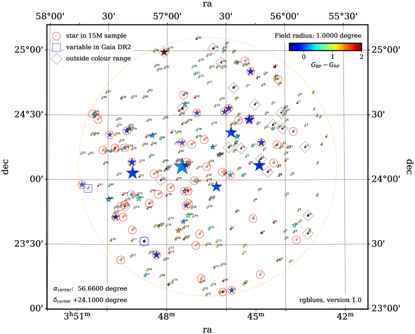
Figure 9: Example of finding chart generated by the Python package rgblues after performing a cone search centred in the Pleiades star cluster, with a search radius of 1°. The stars in this plot are colour coded based on the $G_{\rm BP}^{\rm Gaia}\!-\!G_{\rm RP}^{\rm Gaia}$ colour. A red circle has been overplotted on the stars belonging to the 15M star sample, a blue square on the variable objects in DR2, and a grey diamond on EDR3 stars outside the $-0.5<G_{\rm BP}^{\rm Gaia}\!-\!G_{\rm RP}^{\rm Gaia}<2.0$ mag colour interval. Stars brighter than a pre-defined threshold are displayed with big star symbols. The stars are numbered with labels of different colours (red, blue and black for stars in the 15M star sample, variable objects in DR2, and remaining stars in EDR3, respectively), matching the order of the stars in the three output CSV files generated during the execution of the program.

Trying to help future users of the 15M star sample to perform cone search queries as that shown in the previous subsection, we have also created a Python package, called rgblues, that executes this type of queries and performs the additional extra work required to automatically discriminate between reference stars, belonging to the 15M star sample, from secondary calibrating stars (additional objects in EDR3), flagging objects detected to be variable in Gaia DR2 and those outside the colour range $-0.5<G_{\rm BP}^{\rm Gaia}\!-\!G_{\rm RP}^{\rm Gaia}<2.0$ mag.

Once installed, the software can be easily executed from the command line:
$ rgblues 56.66 24.10 1.0 12
The four positional arguments correspond to RA, DEC, search radius (these three parameters in decimal degrees) and limiting $G^{\rm Gaia}$ magnitude.

The steps followed by rgblues to complete its tasks are the following:

1. cone search in Gaia EDR3 down to a pre-defined limiting $G^{\rm gaia}$ magnitude, gathering the following parameters: source_id, ra, dec, phot_g_mean_mag, phot_bp_mean_mag and phot_rp_mean_mag. In this case, an ADQL query similar to that shown in Sect. A.1 is performed, without imposing any $G_{\rm BP}^{\rm Gaia}\!-\!G_{\rm RP}^{\rm Gaia}$ colour restriction nor evaluating the polynomial transformations given in Eqs. (2)–(5).

2. cone search in the StarHorse sample through the Gaia archive hosted by the Leibniz-Institute for Astrophysics Potsdam. This step, which is optional, allows the compilation of stellar parameters associated with each star, such as interstellar extinction, metallicity and distance.

3. cross-matching of the previous EDR3 sample with the list of 15M star sample from this work. This step determines the subsample of EDR3 stars for which the RGB photometric calibration is reliable.

4. cone search in Gaia DR2. This additional step is performed to retrieve the phot_variable_flag parameter indicating whether the star was flagged as variable in DR2. Note that this flag is not available in EDR3.

5. cross-matching between DR2 and EDR3 to identify the variable stars in EDR3. This step is required because it is not guaranteed that the same astronomical source will always have the same source identifier in the different Gaia Data Releases.

6. computation of the RGB magnitudes using the polynomial transformations given in Eqs. (2)–(5).

7. generation of the output files. Three files (in CSV format) are generated, segregating the star list in i) stars belonging to the 15M star sample (with reliable RGB magnitude estimates), ii) objects flagged as variable in Gaia DR2, and iii) remaining objects in Gaia EDR3. Note that the RGB magnitudes estimated for the latter can be potentially biased due to systematic effects introduced by interstellar extinction, or by exhibiting non-solar metallicity or a colour outside the $-0.5<G_{\rm BP}^{\rm Gaia}\!-\!G_{\rm RP}^{\rm Gaia}<2.0$ mag interval.

8. creation of a finding chart. Fig. 9 illustrates the resulting plot after executing the Python code with the same cone-search parameters employed in Sect. A.1.

References

- Anders et al. (2019) Anders F., et al., 2019, A&A, 628, A94
- Astropy Collaboration et al. (2013) Astropy Collaboration et al., 2013, A&A, 558, A33
- Astropy Collaboration et al. (2018) Astropy Collaboration et al., 2018, AJ, 156, 123
- Bohlin et al. (2014) Bohlin R. C., Gordon K. D., Tremblay P. E., 2014, PASP, 126, 711
- Bravo Alfaro et al. (1997) Bravo Alfaro H., Arellano Ferro A., Schuster W. J., 1997, PASP, 109, 958
- Breddels & Veljanoski (2018) Breddels M. A., Veljanoski J., 2018, A&A, 618, A13
- Cardelli et al. (1989) Cardelli J. A., Clayton G. C., Mathis J. S., 1989, ApJ, 345, 245
- Cardiel et al. (2021) Cardiel N., et al., 2021, MNRAS, 504, 3730
- Castelli & Kurucz (2003) Castelli F., Kurucz R. L., 2003, in Piskunov N., Weiss W. W., Gray D. F., eds, IAU Symposium Vol. 210, Modelling of Stellar Atmospheres. p. A20 (arXiv:astro-ph/0405087)
- Gaia Collaboration et al. (2016) Gaia Collaboration et al., 2016, A&A, 595, A1
- Gaia Collaboration et al. (2021) Gaia Collaboration et al., 2021, A&A, 649, A1
- Górski et al. (2005) Górski K. M., Hivon E., Banday A. J., Wandelt B. D., Hansen F. K., Reinecke M., Bartelmann M., 2005, ApJ, 622, 759
- Harris et al. (2020) Harris C. R., et al., 2020, Nature, 585, 357
- Hoffleit (1964) Hoffleit D., 1964, Catalogue of Bright Stars. Yale University Observatory
- Hunter (2007) Hunter J. D., 2007, Computing in Science Engineering, 9, 90
- Ivezić et al. (2020) Ivezić Z., Connolly A. J., VanderPlas J. T., Gray A., 2020, Statistics, Data Mining, and Machine Learning in Astronomy: A Practical Python Guide for the Analysis of Survey Data. Princeton University Press, https://press.princeton.edu/books/ebook/9780691197050/statistics-data-mining-and-machine-learning-in-astronomy
- Jiang et al. (2013) Jiang J., Liu D., Gu J., Süsstrunk S., 2013, in 2013 IEEE Workshop on Applications of Computer Vision (WACV). pp 168–179, doi:10.1109/WACV.2013.6475015
- Johnson & Mitchell (1975) Johnson H. L., Mitchell R. I., 1975, Rev. Mex. Astron. Astrofis., 1, 299
- Kiehling (1987) Kiehling R., 1987, A&AS, 69, 465
- O’Donnell (1994) O’Donnell J. E., 1994, ApJ, 422, 158
- Osuna et al. (2008) Osuna P., et al., 2008, IVOA Astronomical Data Query Language Version 2.00, IVOA Recommendation 30 October 2008 (arXiv:1110.0503), doi:10.5479/ADS/bib/2008ivoa.spec.1030O
- Pérez & Granger (2007) Pérez F., Granger B. E., 2007, Computing in Science and Engineering, 9, 21
- Queiroz et al. (2018) Queiroz A. B. A., et al., 2018, MNRAS, 476, 2556
- R Core Team (2021) R Core Team 2021, R: A Language and Environment for Statistical Computing. R Foundation for Statistical Computing, Vienna, Austria, %****␣paper_RGB_Gaia.bbl␣Line␣150␣****https://www.R-project.org/
- Riello et al. (2021) Riello M., et al., 2021, A&A, 649, A3
- STScI development Team (2018) STScI development Team 2018, synphot: Synthetic photometry using Astropy (ascl:1811.001), https://synphot.readthedocs.io/en/latest/
- Schuster (1976) Schuster W. J., 1976, Rev. Mex. Astron. Astrofis., 1, 327
- Virtanen et al. (2020) Virtanen P., et al., 2020, Nature Methods, 17, 261
- Wes McKinney (2010) Wes McKinney 2010, in Stéfan van der Walt Jarrod Millman eds, Proceedings of the 9th Python in Science Conference. pp 56 – 61, doi:10.25080/Majora-92bf1922-00a
- Zonca et al. (2019) Zonca A., Singer L., Lenz D., Reinecke M., Rosset C., Hivon E., Gorski K., 2019, Journal of Open Source Software, 4, 1298
- van der Sluys (2005) van der Sluys M., 2005, Constellation lines, https://github.com/hemel-waarnemen-com/Constellation-lines