A modular U-Net for automated segmentation of X-ray tomography images in composite materials

Abstract

XCT techniques have evolved to a point that high-resolution data can be acquired so fast that classic segmentation methods are prohibitively cumbersome, demanding automated data pipelines capable of dealing with non-trivial 3D images. Deep learning has demonstrated success in many image processing tasks, including material science applications, showing a promising alternative for a human-free segmentation pipeline. In this paper a modular interpretation of U-Net (Modular U-Net) is proposed and trained to segment 3D tomography images of a three-phased glass fiber-reinforced Polyamide 66 . We compare 2D and 3D versions of our model, finding that the former is slightly better than the latter. We observe that human-comparable results can be achievied even with only 10 annotated layers and using a shallow U-Net yields better results than a deeper one. As a consequence, NN show indeed a promising venue to automate XCT data processing pipelines needing no human, adhoc intervention.

XCT, a characterization technique used by material scientists for non-invasive analysis, has tremendously progressed over the last 10 years with improvements in both spatial resolution and throughput [1, 2]. Progress with synchrotron sources, including the recent European Synchrotron Radiation Facility (ESRF) upgrade [3], made it possible to look inside a specimen without destroying it in a matter of seconds [4] – sometimes even faster [5].

This results in a wealth of 3D tomography images (stack of 2D images) that need to be analyzed and, in some applications, it is desirable to segment them (i.e. transform the gray-scaled voxels in semantic categorical values). A segmented image is crucial for quantitative analyses; for instance, measuring the distribution of precipitate length and orientation [6], or phase characteristics, which can be useful for more downstream applications like estimating thermo-mechanical properties [7].

XCT images typically have billions of voxels, weighting several gigabytes, and remain complex to inspect manually even using dedicated costly software (e.g.: Avizo , VGStudioMax ). Using thresholds on the gray level image is an easy, useful method to segment phases in tomographies, but it fails in complex cases, in particular when acquisition artifacts (e.g.: rings, beam hardening, phantom gradients) are present. Algorithms based on mathematical morphology like the watershed segmentation [8, 9] help tackling more complex scenarios, but they need human parametrization, which often requires expertise in the application domain. Thus, scaling quantitative analyses is expensive, creating a bottleneck to process 3D XCT – or even 4D (3D with time steps).

Deep Learning approaches offer a viable solution to attack this issue because NNs can generalize patterns learned from annotated data. A NN is a statistical model originated from perceptrons [10] capable of approximating a generic function. Convolutional s [11], a variation adapted to spatially-structured data (time series, images, volumes), made great advances in computer vision tasks. Since the emergence of popular frameworks like TensorFlow [12], more problem-specific architectures have been proposed, such as Fully-convolutional NNs [13], a convolution-only type of model used to map image pixel values to another domain (e.g. classification or regression).

[6] trained a model to segment three phases in 3D nanotomographies of an Al-Cu alloy, showing that even a simple CNN can reproduce patterns of a human-made segmentation. [14] optimized a SegNet [15] to segment dendrites of different alloys, including a 4D XCT. [7] identified Aluminides and Si phases in XCT using a U-Net, an architecture that, along with its many flavors [16, 17, 18, 19], has shown success in a variety of applications [20, 21, 22]. Finally, [23] combined U-Nets with classic segmentation algorithms (e.g. marker-based watershed) to segment grain boundaries in successive XCTs of an Al-Cu specimen as it is submitted to Ostwald ripening steps.

In this paper, an annotated 3D XCT of glass fiber-reinforced Polyamide 66 is presented as an example of segmentation problem in Materials Science that can be automated with a deep learning approach. Our NN architecture, the Modular U-Net (Fig. 2 and Fig. 3), is proposed as a generalized representation of the U-Net, explicitly factorizing the U-like structure from its composing blocks.

Like [23], we compare three variants on the composite material dataset focusing on the dimensionality of the convolutions (2D or 3D), obtaining qualitatively human-like segmentation (Fig. 1 and Fig. 4) with all of them although 2D-convolutions yield better results (Fig. 5(a)). We find that (for the considered material) the U-Net architecture can be shallow without loss of performance, but batch normalization is necessary for the optimization (Fig. 5(b)). Finally, a model’s learning curve (Fig. 6) shows that only ten annotated 2D slices are necessary to train our NN.

Our results show that NNs can be not only a quality-wise satisfactory but also a viable solution in practice for XCT segmentation as it requires relatively little annotated data and shallow models (therefore faster to train).

1 Data

Figure 1: Segmentation on the test set. Color code: blue represents voxels correctly classified as fiber (hatched), yellow as porosity (contours), and red represents misclassification. Supplementary video: youtu.be/HvdWhDZJgLE.

The data used in this work is composed of synchrotron X-ray tomography volumes recorded using $2\text{\,}\mathrm{mm}$ $\times$ $2\text{\,}\mathrm{mm}$ cross section composite specimens of Polyamide 66 reinforced by glass fibers. A volume of $2048^{3}$ voxels, referred to as Train-Val-Test (Fig. 1 and Fig. 7), was cropped to get rid of the specimen’s borders, and its ground truth segmentation was created semi-manually with ImageJ [24] (using Fiji [25]) and Avizo. The tomography of another specimen of the same material was also processed and partially annotated in order to evaluate our models (Fig. 4) – it is further referred to as the crack volume because of the fracture inside it. Both image volumes and the former’s annotations are publicly available [26].

Acquisition

X-ray tomography scans were recorded on the Psiché beamline at the Synchrotron SOLEIL using a parallel pink beam. The incident beam spectrum was characterized by a peak intensity at $25\text{\,}\mathrm{keV}$, defined by the silver absorption edge, with a full width at half maximum bandwidth of approximately $1.8\text{\,}\mathrm{keV}$. The total flux at the sample position was about $2.8\text{\times}{10}^{12}\text{\,}\mathrm{p}\mathrm{h}\mathrm{o}\mathrm{t}\mathrm{o}\mathrm{n}\mathrm{s}\mathrm{/}\mathrm{s}\mathrm{/}\mathrm{m}\mathrm{m}^{2}$. The detector placed after the sample was constituted by a LuAG scintillator, a 5$\times$ magnifying optics, and a Hamamatsu CMOS 2048 x 2048 pixels detector (effective pixel size of $1.3\text{\,}\mathrm{\SIUnitSymbolMicro m}$). 1500 radiographs were collected over a $180\mathrm{°}$ rotation and an exposure of $50\text{\,}\mathrm{m}\mathrm{s}$ (full scan duration of 2 minutes). The sets of radiographs were then processed using PyHST2 reconstruction software [27] with the Paganin filter [28] activated to enhance the contrast between the phases.

Phases

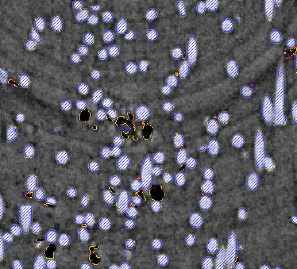
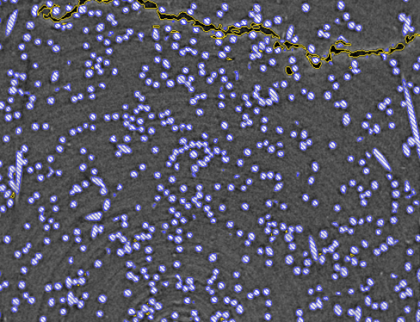
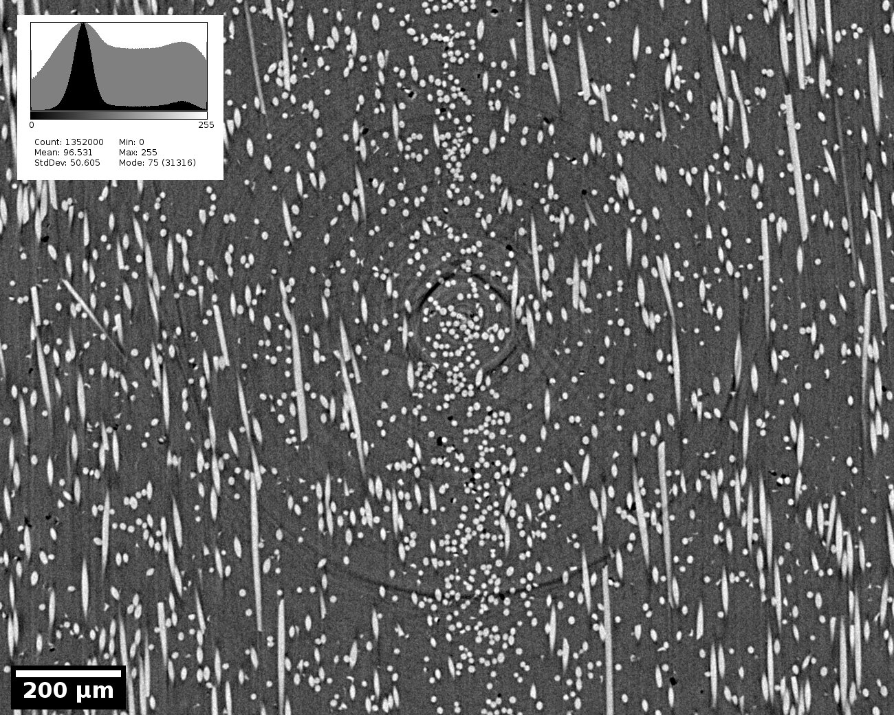
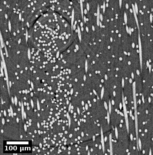
The three phases present in the material are visible in Fig. 1: the polymer matrix (gray), the glass fibers (white, hatched in blue), and damage in form of pores (dark gray and black, contoured in yellow) – referred as porosity here. One can observe that the orientation of the fibers is unevenly distributed; they are mostly along the axes Y (vertical) and Z (out of the plane) in Fig. 7.

Ground truth

The data was annotated in two steps: first, the fiber and the porosity phases were independently segmented using Seeded Region Growing [29]; then, ring artifacts that leaked to the porosity class were manually corrected. A detailed description of the procedure is presented in the A.

Data split

The ground truth layers (of the Train-Val-Test volume) were sequentially split – their order were preserved to train the 3D models (Section 2.2) – into three sets: train (1300 layers), validation (128 layers), and test (300 layers). A margin of 86 layers between these sets was adopted to avoid information leakage. The train layers were used to train the NNs, the validation layers were used to select the best model (during the optimization), and the test layers were used to evaluate the models (Section 3).

Class imbalance

Due to the material’s nature, the classes (phases) in this dataset are intrinsically imbalanced. The matrix, the fiber, and the porosity represent, respectively, 82.3%, 17.2%, and 0.5% of the voxels.

2 Neural Network

Problem formulation

Let $\>x\in\mathcal{X}=\interval{0}{1}^{w\times 0pt\times 0pt}\>$ be a normalized gray 3D image. Its segmentation $\>y\in\mathcal{Y}=\llbracket C\rrbracket^{w\times 0pt\times 0pt}\>$, where $\>\llbracket C\rrbracket=\{0,1,\dots,C-1\}\>$, contains a class value in each voxel, which may represent any categorical information, such as the phase of the material. In this setting, a segmentation algorithm is a function $\>f:\mathcal{X}\to\mathcal{Y}\>$. In this section we present our approach (that is, the $\>f\>$) used to segment the data described in the previous section.

First, a generic U-Net architecture, which we coined Modular U-Net (Fig. 2), is proposed; then, the modules used in this work are briefly exposed (detailed description and hyperparameters in the B); finally, three variations of the Modular U-Net, based on the input, convolution, and output nature (2D or 3D), are presented. Our training setup (loss function, optimizer, learning rate, data augmentation, implementation framework, and hardware) is described in C.

2.1 Modular U-Net

Since [16] proposed U-Net, variations of it emerged in the literature (e.g.: [17, 18]). Here we propose a generalized version, preserving its overall structure. The Modular U-Net (Fig. 2) is based on three blocks: the Convolutional Block (ConvBlock), the Downsampling Block (DownBlock), and the Upsampling Block (UpBlock).

The left/right side of the architecture corresponds to an encoder/decoder, a repetition of pairs of ConvBlock and DownBlock/UpBlock modules. They are connected by concatenations between their respective parts at the same U-level – which corresponds to the inner tensors’ resolutions (higher U-level means lower resolution). The U-depth, a hyperparameter, is the number of U-level s in a model, corresponding to the number of DownBlock (and equivalently UpBlock) modules.

Figure 2: Modular U-Net: a generalization of the U-Net architecture.

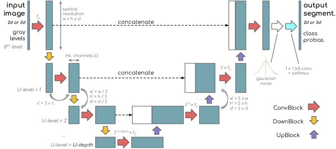
The ConvBlock is a combination of operations that outputs a tensor with the same spatial dimensions of its input, though the number of channels may differ – in our models it always doubles. The assumption of equally-sized input/output is optional, but we admit it for the sake of simplicity because it makes the model easier to be used with an arbitrarily shaped volume. The numbers of channels after the ConvBlocks is $\>2^{\text{\lx@glossaries@gls@link{main}{ulevel}{\leavevmode U-level}}}\times f_{0}\>$, where $\>f_{0}\>$ is the number of filters in the first convolution.

The DownBlock/UpBlock divides/multiplies the input tensor’s shape by two in every spatial dimension: width, length, and depth in the 3D case. In other words, a tensor with shape $\>(w,0pt,0pt,c)\>$, where $\>c\>$ is the number of channels, becomes, respectively, $\>(\frac{w}{2},\frac{0pt}{2},\frac{0pt}{2},c)\>$ after a DownBlock and $\>(2w,20pt,20pt,c)\>$ after an UpBlock.

In [16], for instance, the ConvBlock is a sequence of two 3x3 convolutions with ReLU activation, the DownBlock is a max pooling, and the UpBlock is an up-sampling layer. In [17], the ConvBlock is a 3D convolutional layer, and in [18] it is a nested U-Net.

The ConvBlock used here (Fig. 3) is a sequence of two 3x3 (x3 in the 3D case) convolutions with ReLU activation, a residual connection with another convolution, batch normalization before each activation, and dropout at the end. The DownBlock is a $3\times 3$ convolution with $2\times 2$ stride, and the UpBlock is a $3\times 3$ transposed convolution with $2\times 2$ stride.

Figure 3: Examples of Modular U-Net blocks. Left: our ConvBlock. Middle/right: rigid/learnable DownBlock and UpBlock.

2.2 Variations: 2D, 2.5D, and 3D

Since our dataset contains intrinsically 3D structures, we compared the performances of this architecture using 2D and 3D convolutions. The former processes individual tomography z-slices (XY plane) independently, and the latter processes several at once (i.e. a volume).

We also compared an intermediate version, which we coined 2.5D, that processes one tomography z-slice at a time using 2D convolutions, but takes five slices at the input, as if the pairs of data slices above and below were channels of the 2D image. Table 2 summarizes these differences.

The visual characteristics of the z-slices are mostly invariant, and we observed a high correlation between adjacent z-slices; therefore, the 2D and 2.5D models take 2D cuts in the XY plane, as in Fig. 1 Fig. 7.

3 Results

In this section we present a compilation of qualitative and quantitative results obtained. The segmentations from the three Modular U-Net versions presented in Section 2 are quantitatively compared, then an ablation analysis and the learning curve of the 2D model are presented. All the quantitative analyses were made on the test split (see Section 1), which contains $1300\times 1040\times 300\approx$ $406\text{\times}{10}^{6}\text{\,}\mathrm{v}\mathrm{o}\mathrm{x}\mathrm{e}\mathrm{l}\mathrm{s}$. Other images and videos are provided along with further detailed analysis as supplementary material in the D. The trained models and the data used to produce our results are publicly available online [30, 26].

Qualitative results

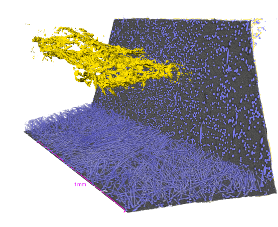
Figure 1 shows two snapshots of the segmentation generated with a 2D model. Figure 4 shows the segmentation obtained with the 2D model from the crack volume, used evaluate its usability in terms of processing speed and applicability of the method to other data. The segmented data was then used to generate a surface of the crack inside it – we refer to it as the crack volume in the next section. Using an NVIDIA Quadro P2000 ($5\text{\,}\mathrm{G}\mathrm{B}$), it took $32\text{\,}\mathrm{m}\mathrm{i}\mathrm{n}\mathrm{u}\mathrm{t}\mathrm{e}\mathrm{s}$ to process a $1579\times 1845\times 2002$ ($\approx$ $5800\text{\,}\mathrm{M}\mathrm{v}\mathrm{o}\mathrm{x}\mathrm{e}\mathrm{l}\mathrm{s}$) volume. This shows that this type of analysis could carried out almost in real time using typical hardware available at a synchrotron beamline.

(a)

(b)

Figure 4: Segmentation of the volume crack. Color code: blue represents the fiber and yellow represents the porosity. Supplementary video: youtu.be/rmBTZrcMrCk. (4(a)) Two orthogonal planes inside the specimen; the fibers are rendered in 3D at the bottom of the volume, and the crack is rendered as a surface. (4(b)) A crop from the vertical plane in a slice passing through the fracture. The fiber segmentation is hatched in blue and the porosity segmentation is contoured in yellow.

Baseline

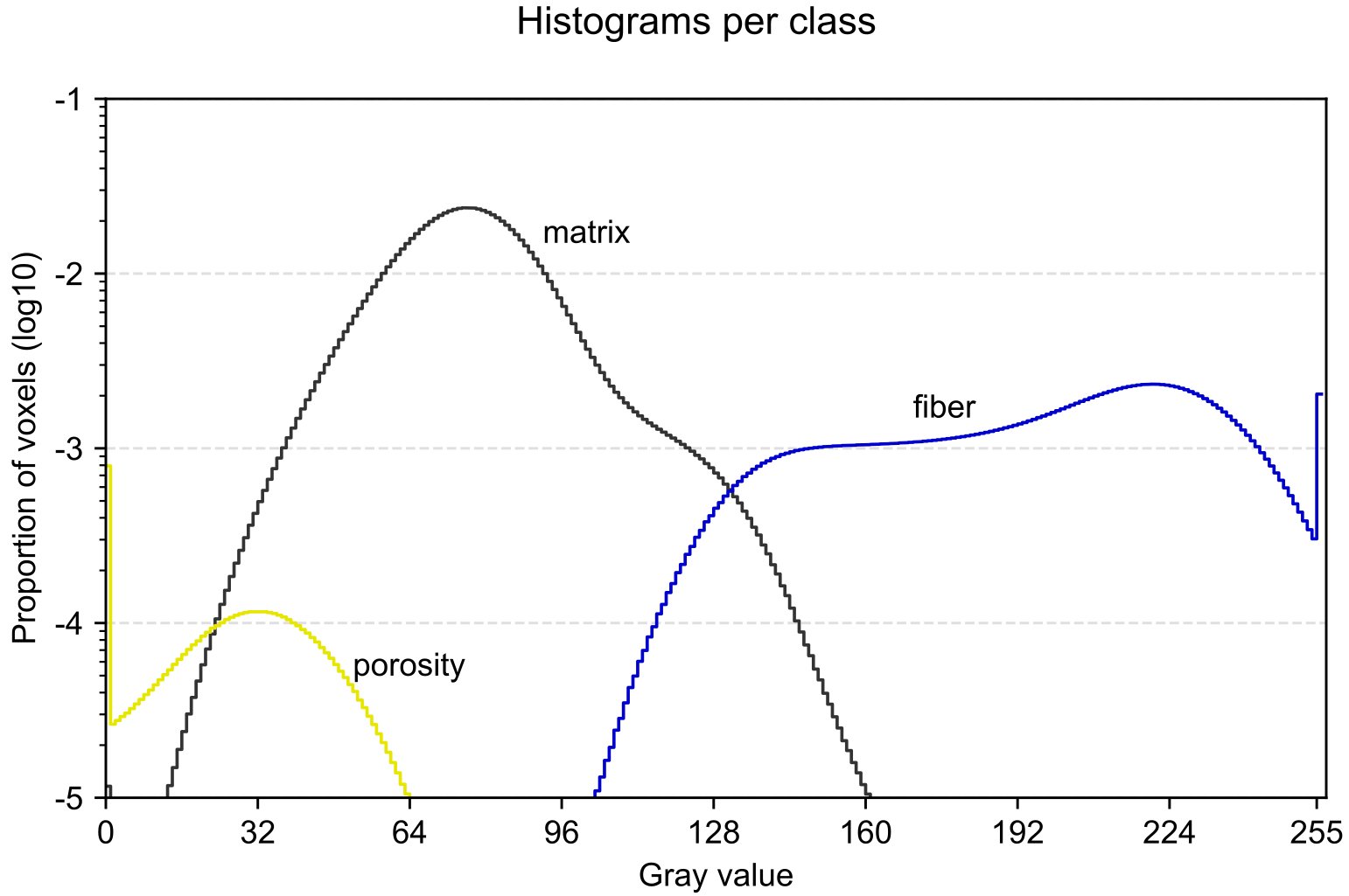
For the sake of comparison, we considered the expected performance of two theoretical models: the ZeroOC and the Bin-wise ZeroOC . The ZeroOC relies only on the class imbalance, while Bin-ZeroOC takes the individual gray values into consideration, leveraging information from the histograms of each class (Fig. 8) – see Table 4 for more details.

Quantitative results

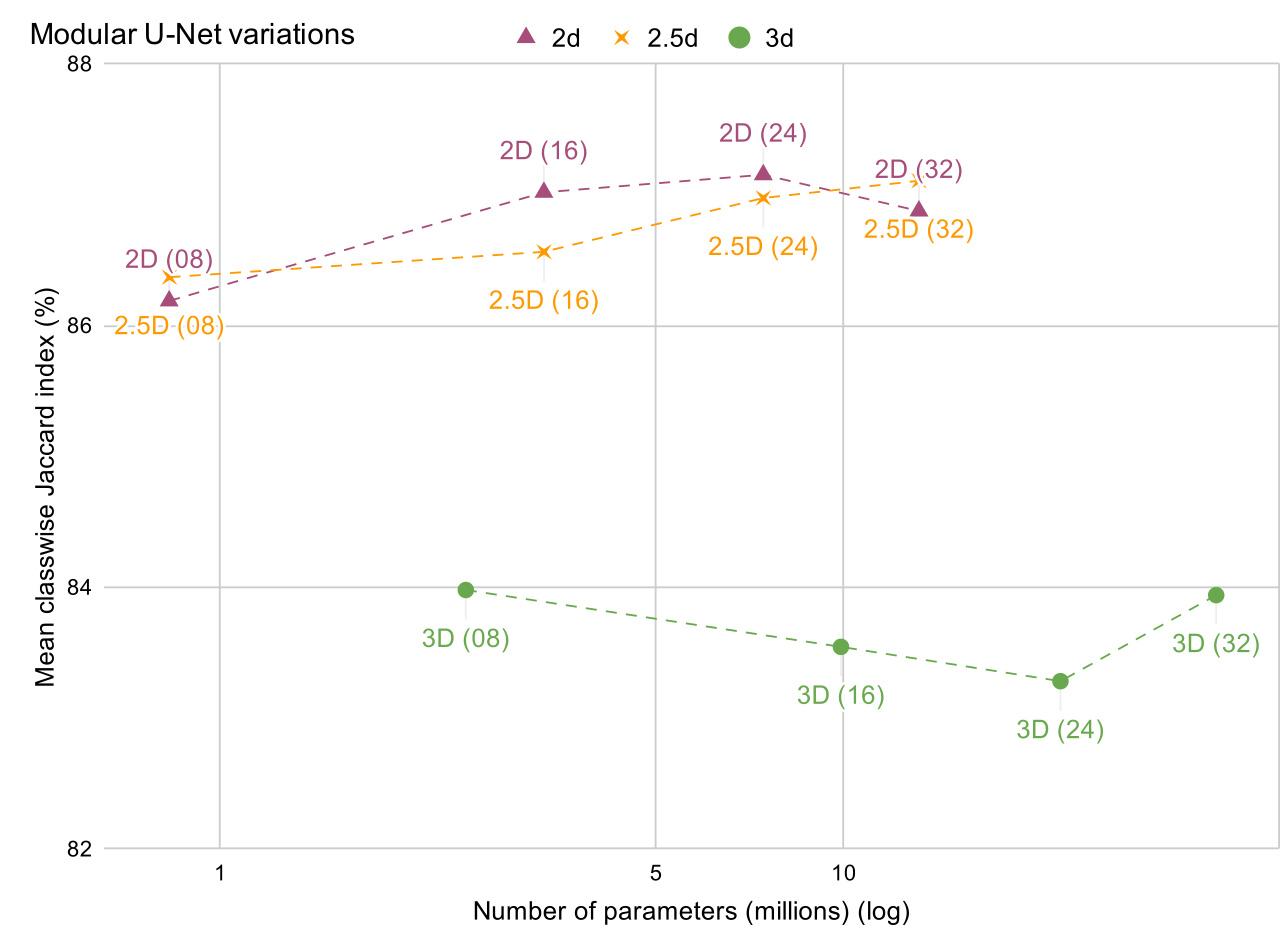
Figure 5 presents a comparison of the three model variations (2D, 2.5D, and 3D) and an ablation study of the 2D model in terms of number of parameters and performance. The three variations of the Modular U-Net are evaluated with varying sizes. The models are scaled with the hyperparameter $\>f_{0}\>$ (values inside the parentheses in Fig. 5(a)).

The performance is measured using the Jaccard index, also known as Intersection over Union (IoU), on each phase (class). Our main metric is the arithmetic mean of the three class-wise indices, and the baseline (minimum) is $76.2$% (Table 4). This metric provides a good visibility of the performance differences and resumes the precision-recall trade off; other classic metrics – even the area under the ROC[31] curve – are close to 100% (see D), so the differences are hard to compare.

(a)

(b)

Figure 5: Modular U-Net variations comparison. On the x-axis, the number of parameters; on the y-axis the mean class-wise Jaccard indices. (5(a)) The Modular U-Net 2D, 2.5D, and 3D versions are scaled with $\>f_{0}\>$ (in parentheses), the number of filters of the first convolution of the first ConvBlock. (5(b)) Components were removed individually, or replaced by alternatives. Removals: dropout, gaussian noise, residual (skip connection), batch normalization (out of scale). Replacements: convolutions by separable ones, learnable DownBlock/UpBlock by rigid ones (Fig. 3), and batch normalization by layer normalization. We also compare the effect of the U-depth, i.e. number of levels in the U structure. Notice that the data point of the batch normalization removal is out of scale in the y-axis for the sake of visualization.

Ablation study

Figure 5(b) is a component ablation analysis of the 2D model with $\>f_{0}=16\>$. Starting with the 2D model with the default hyperparameters (see Fig. 3, and Section B), we retrained other models removing one component at a time. The learnable up/down-samplings were replaced by rigid ones (see Fig. 3), the 2D convolutions were replaced by separable ones, and the batch normalization was replaced by layer normalization. Finally, we varied the U-depth from 2 to 4.

Notice that the model without dropout performed better than the reference model, but we kept it in our default parameters because the same thing did not occur with other variations and sizes.

Learning curve

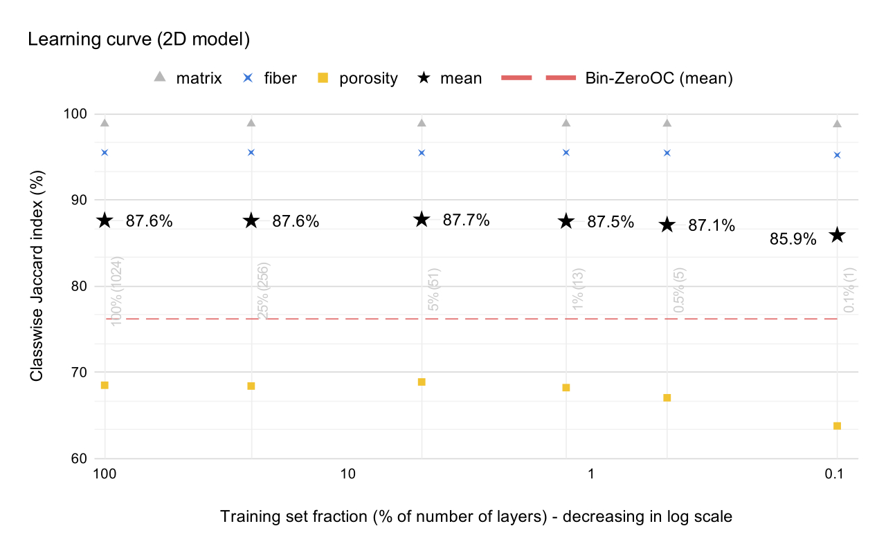
Finally, we computed the learning curve of the 2D model (Fig. 6) logarithmically reducing the size of the train dataset from 1024 z-slices until a single layer.

Figure 6: Learning curve of the 2D model with default hyperparameters (B).

4 Discussions

4.1 Overview

Our models, trained in one to three hours, achieved, qualitatively, very satisfactory results from a Materials Science application point of view, with 87% of mean class-wise Jaccard index and an F1-score macro average of 92.4% (Table 5). We stress the fact that these results were achieved without any strategy to compensate the (heavy) class imbalance (82.3% of the voxels belong to the class matrix); they may be further improved using, for instance, re-sampling strategies [32, 33], class-balanced loss functions [34, 35], or self-supervised pre-training [36].

The results obtained with another specimen (the crack volume), thus with slight variations in the acquisition conditions, were of good quality (inspection by an expert showed no visible error in the segmentation) and way faster than the manual process. The crack was mostly, and correctly, segmented as porosity without retraining the model, showing its capacity to generalize – an important feature for its practical use, although some misclassified regions can be seen as holes (missing pieces) in the fracture’s surface (Fig. 4(a)).

Moreover, the processing time achieved ($32\text{\,}\mathrm{m}\mathrm{i}\mathrm{u}\mathrm{t}\mathrm{e}\mathrm{s}$) is indeed a promising prospect compared to classic approaches.

4.2 Segmentation errors

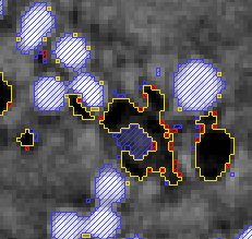
As highlighted in Fig. 1, the model’s mistakes (in red), are mostly on the interfaces of the phases, which are fairly comparable to a human annotator’s. We (informally) estimate that they are in the error margin because, in some regions, there is no clear definition of the phases’ limits. The fibers may show smooth, blurred phase boundaries with the matrix, while part of the porosities are under the image resolution.

Another issue is the loss of information (all-zero regions) in some rings (e.g.: Fig. 7(b)). In such cases, even though one could deduce that there is indeed a porosity, it is practically impossible to draw a well-defined porosity/matrix interface.

Finally, we reiterate that the ground truth remains slightly imperfect despite our efforts to mitigate these issues. For instance, in Figure 1 we see, inside the C-like shaped porosity, a blue region, meaning that it was correctly segmented as a fiber – yet, there is no fiber in it.

4.3 Model variations

Figures 9 and 6 confirm that, no matter the model variation, the porosity is harder to detect. Although, the qualitative results are reasonable, and we underline that the Jaccard index is more sensitive on underrepresented classes because the size of the union will always be smaller (see Equation 1).

Contrarily to our expectations, Figure 5(a) shows that the 2D model performed systematically better than the 3D (albeit the difference is admittedly small). We expected the 3D model to perform better because the morphology of the objects in the image are naturally three-dimensional; besides, other work [23] have obtained better results in binary segmentation problems. We raise two hypotheses about this result: (1) the set of hyperparameters is not optimal, and (2) the performance metric is biased because the annotation process uses a 2D algorithm.

4.4 Model ablation

Figure 5(b) contains a few interesting findings about the hyperparameters of the Modular U-Net:

1. using learnable up/down-sampling operations indeed gives more flexibility to the model, improving its performance compared to rigid (not learnable) operations;

2. separable convolutions slightly hurt the performance, but it reduces the number of parameters by 60%;

3. decreasing the U-depth, therefore shrinking the receptive field, improved the performance while reducing $75\%$ of the model size; on the other hand, increasing the depth had the opposite effect, multiplying the model size by four, while degrading the performance;

4. batch normalization is essential for the training – notice that the version without batch normalization is out of scale in Fig. 5(b), and its performance corresponds to the ZeroOC model (Table 4);

Model depth (item 3)

This finding gives a valuable information for our future work because using shallower models require less memory (i.e.: bigger crops can be processed at once), making it possible to accelerate the processing time. We hypothesize that the necessary receptive field is smaller than the depth-three model’s. Therefore, a spatially bigger input captures irrelevant, spurious context to the classification.

4.5 Learning curve

Figure 6 highlights the most promising finding in our results. Our model was capable of learning with only 1% of the training dataset (about ten z-slices) even with no smart strategy to select the layers in the experiment (the training volume was sequentially reduced along the z-axis), and even a single layer was sufficient to achieve nearly the same performance.

5 Conclusion

An annotated dataset of a three-phase composite material was presented, and a reinterpretation of the U-Net architecture as a modularized structure was proposed as a solution to scale up the segmentation of such images. Our models achieved satisfactory results showing a promising venue to automate processing pipelines of XCTs of this material with only a few annotated tomography slices. The Modular U-Net is a conceptually more compact interpretation of its precursor, providing a more abstract representation of this family of network architectures.

2D and 3D versions of the Modular U-Net were compared, showing that both were capable of learning the patterns in a human-made annotation, but the former was systematically better than the latter. An ablation study provided insights about the hyperparameters of our architecture, especially revealing that we might further accelerate the processing with smaller models. We also qualitatively analyzed the usability of our models on an image of a different specimen, confirming that it is a viable solution.

Our code is available on GitHub , and the data and trained models referred here are publicly available on Zenodo [26, 30].

6 Future work

Carrying on the encouraging results found in this work, we envision scaling up the use of our models to process other volumes and 4D XCTs. We also plan identifying better strategies to deal with ill-defined regions (e.g.: matrix/fiber blurred interfaces), an issue modestly mitigated in our work, to improve our approach’s usability. Two possibilities are considered: (1) post-processing the class probabilities to detect bad predictions, for instance using the method proposed by [37]; (2) define a special class for uncertain regions. Finally, we might as well search for better ways to measure a prediction’s consistency with respect to the objects’ 3D morphology.

7 Acknowledgement

João P C Bertoldo would like to acknowledge funding from the BIGMÉCA research initiative, funded by Safran and MINES ParisTech. Henry Proudhon would like to acknowledge beam time allocation at the Psiché beamline of Synchrotron SOLEIL for the proposal number 20150371.

Appendix A Data: further details

(a) A $1300\times 1040$ slice on the XY plane of the volume Train-Val-Test. On the upper left corner, a histogram of the gray level values in the image; linear scale in black, log scale in gray.

(b) Zoom. Ring artifacts, from the acquisition process, can be as dark as porosities, making it harder to segment such regions.

Figure 7: Glass fiber-reinforced Polyamide 66 raw tomography. Supplementary video: youtu.be/4kifxlvxzb8.

A.1 Data annotation

We annotated the data in two phases. First, the fiber and the porosity were separated from the matrix independently using Seeded Region Growing [29]. As the results carried a considerable amount of artifacts in the porosity phase, we manually corrected them with a second procedure.

Data annotation step 1: Seeded Region Growing [29]

To generate the seeds, we applied contrast and brightness transformations to enhance the information on the phase of interest, then applied Non-Local Means [38, 39] to attenuate the ring artifacts, and finally used manual thresholds to select easy voxels (mostly, regions without class superposition in Fig. 8). Finally, we run it on each tomography z-slice independently.

We observed that some regions were poorly segmented due to the ring artifacts, creating false, larger porosities. To mitigate this issue, we manually corrected part of the artifacts, reducing their size while keeping it consistent with adjacent z-slices.

Data annotation step 2: artifacts correction

We separated 2D blobs (connected components) in the porosity phase, then extracted region properties (e.g.area, aspect ratio, etc) to find outliers – mostly, porosities significantly larger than the average. Using Avizo, we then corrected imperfections manually editing the annotation. Most problematic regions were on pronounced rings, where it is hard to define the borders of a porosity (e.g.: Fig. 7), so we cleaned ill-defined porosities conservatively shrinking their volume/borders based on the layers above and below.

A.2 Ground truth analysis

Class-wise histogram

Figure 8 shows a normalized gray level histogram per class (the normalization is relative to all the classes confounded). Using a threshold approach is naturally prone to imprecise results because a voxel’s gray value is insufficient to determine its class. This illustrates how this volume cannot be segmented using a threshold. An example can be seen in Fig. 7(b), where the rings are as dark as the porosities.

Figure 8: Glass fiber-reinforced Polyamide 66 gray value (normalized) histograms (one per class). The histogram is normalized globally, i.e. a bin’s value is the proportion of voxels out of all the voxels (all classes confounded). The superposition of the classes’ value ranges make it impossible to segment the image with a threshold on the gray values.

A.3 Data availability

The volumes mentioned here (Table 1) are available on Zenodo [40]. Notice that the volumes (1) and (1) contain all the three splits (train, validation, test) together (1900 z-slices), while the volumes (1) and (1) correspond to their last 300 z-slices. The values in the segmentation volumes (predictions and ground truth) are 0, 1, and 2, which respectively correspond to the phases matrix, fiber, and porosity. The volumes (1) and (1) correspond to the volume in Fig. 4. The .raw files have complementary .raw.info files containing metadata (volume dimensions and data type) about its respective volume.

Table 1: Published 3D volumes: all the data necessary to train and test the models presented in this paper are publicly available on Zenodo [26]. A demo of how to read the data is available on GitHub.

.zip file	.raw file	Description
pa66.zip	pa66.raw (a)	Data (gray level image stack) of the Train-Val-Test volume.
	pa66.ground_truth.raw (b)	Ground truth segmentation of the Train-Val-Test volume.
pa66_test.zip	pa66.test.prediction.raw (c)	Segmentation generated by the best 2D model on the test set.
	pa66.test.error_volume.raw (d)	Disagreement between the ground truth and the model’s prediction on the test set: 1 means incorrect, 0 means correct.
crack.zip	crack.raw (e)	Data of the non-annotated volume containing a crack inside.
	crack.prediction.raw (f)	Segmentation generated with the best 2D model on the crack volume.

Figure 7 was generated in Fiji [25] with the volume (1). Figure 1 was generated in Avizo with volumes (1) and (1), which is derived from volumes (1) and (1). Figure 4(b) was generated in Avizo with volumes (1) and (1). All the supplementary videos were generated in Avizo.

Appendix B Default hyperparameters

Parameters not mentioned are the default in TensorFlow 2.2.0.

Table 2: Modular U-Net variations: input, convolutional layer, and output nature (2D or 3D).

Model	Input (data)	Convolution	Output (segm.)
2D	2D	2D	2D
2.5D	3D	2D	2D
3D	3D	3D	3D

Table 3: Default hyperparameters.

Parameter	2D	2.5D	3D
U-depth	3	3	3
Convolution kernel	3 $\times$ 3	3 $\times$ 3	3 $\times$ 3 $\times$ 3
Batch size	10	10	10
Crop shape	160 $\times$ 160	160 $\times$ 160 $\times$ 5	32 $\times$ 32 $\times$ 32
Dropout	10%	10%	10%
Gaussian noise (zero mean) standard deviation	0.03	0.03	0.03
f0	16	16	16
Up/Down-sampling stride or Max pooling size	2 $\times$ 2	2 $\times$ 2	2 $\times$ 2 $\times$ 2
BatchNorm momentum	0.5	0.5	0.5

Appendix C Training

Loss function

We trained our models using a custom loss inspired on the Jaccard index, also known as IoU.

Def. 1.

Let $\>A\>$ and $\>B\>$ be two discrete sets. The Jaccard index $\>J\in\interval{0}{1}\>$ is

$$J(A,B)=\frac{|A\cap B|}{|A\cup B|}=\frac{|A\cap B|}{|A|+|B|-|A\cap B|}$$ (1)

We adapt, similarly to [41], the second form in Equation 1 to define the multi-class $Jaccard^{2}$ loss for a batch of voxels (a batch of 2D or 3D images unraveled on the spatial dimensions) as follows.

Def. 2.

Let $\>{y}_{i}\in\{0,1\}^{C}\>$ be the one-hot-encoding ground truth vector of the voxel at position $\>i\in\llbracket B\rrbracket\>$ in a batch of $\>B\>$ voxels $\>y\in\{0,1\}^{B\times C}\>$, where $\>{y}_{ic}\in\{0,1\}\>$ is its value in the $\>c\text{-th}\>$ position.

$${y}_{ic}=\begin{cases}1,&\text{if the voxel $i$ belongs to the class}\;c\in\llbracket C\rrbracket\\ 0&\text{otherwise}\end{cases}$$

A model’s last activation map, a per-voxel softmax, is a tensor $\>\hat{y}\in\interval{0}{1}^{B\times C}\>$, where each row is a probability vector $\>{\hat{y}}_{i}\in\interval{0}{1}^{C}\>$, and the component $\>{\hat{y}}_{ic}$ corresponds to the probability assigned to the class $\>c\>$.

The $Jaccard^{2}$ loss $\>J2\in\interval{0}{1}\>$ of the batch $\>(y,\hat{y})\>$ is

$$J2(y,\hat{y}) =1-\frac{\sum_{i=1}^{N}\sum_{c=1}^{C}{y}_{ic}{\hat{y}}_{ic}}{\sum_{i=1}^{N}\sum_{c=1}^{C}{y}_{ic}{y}_{ic}+\sum_{i=1}^{N}\sum_{c=1}^{C}{\hat{y}}_{ic}{\hat{y}}_{ic}-\sum_{i=1}^{N}\sum_{c=1}^{C}{y}_{ic}{\hat{y}}_{ic}}$$ (2)

$$=1-\frac{\sum_{i=1}^{N}{\hat{y}}_{i*}}{N+\sum_{i=1}^{N}\left(\left(\sum_{c=1}^{C}{\hat{y}}_{ic}^{2}\right)-{\hat{y}}_{i*}\right)}$$ (3)

where $\>{\hat{y}}_{i*}=\sum_{c=1}^{C}{y}_{ic}{\hat{y}}_{ic}\>$ is the probability assigned to the correct class of the voxel $\>i$.

Notice that the $\>J2\in\interval{0}{1}$, which is convenient because it can be expressed as a percentage. $\>J2=100\%\>$ is a completely uncorrelated estimation, and $\>J2=0\%\>$ is a perfect replication of the ground truth.

Optimizer and Learning Rate

We used AdaBelief [42], an optimizer that combines the training stability and fast convergence of adaptive optimizers (e.g.: Adam [43]) and good generalization capabilities of accelerated schemes (e.g.: Stochastic Gradient Descent (SGD) [44]). We used a learning rate of $10^{-3}$ for 100 epochs (10 batches each with batch size 10), followed by a linearly decaying rate until $10^{-4}$ in another 100 epochs. Adam gave equivalent results but took longer (more epochs) to converge.

Data augmentation

In order to increase the variability of the data, random crops are selected from the data volume, then a random geometric transformation (flip, $90\mathrm{°}$ rotation, transposition, etc) is applied. As our training dataset is reasonably large, we used a simple data augmentation scheme, but richer transformations may be applied as long as the transformations result in credible samples.

Implementation and hardware

We trained our models using Keras [45] with TensorFlow’s [12] GPU-enabled version with CUDA $10.1$ running on two NVIDIA Quadro P4000 (2x $8\text{\,}\mathrm{G}\mathrm{B}$). The implementation of our experiments is available on GitHub .

Appendix D Further results

In this section we present complementary performance metrics, images, and videos from the segmentation generated by the 2D model (see Section 2) using our default hyperparameters (B) on the test split. Videos are available as supplementary material.

Table 4 presents the expected performances of the two baseline models we considered (Section 3).

Table 4: Expected performance of baseline theoretical models in terms of class-wise Jaccard index (%).

Model	Description	Matrix	Fiber	Porosity	Mean
ZeroOC	Classify every voxel with the majority class (matrix).	81.0	0	0	27.0
Bin-ZeroOC	Classify a voxel based only on its value. The majority class of each value is chosen. This is equivalent to a ZeroOC model per gray level.	98.4	94.2	35.9	76.2

Table 5 shows a report with classic classification metrics and the Jaccard index by class along with their macro/micro averages. As one can see, the accuracy, precision, and recall of the matrix and the fiber are all close to 100%, while the porosity’s scores are considerably lower.

Table 5: 2D Modular U-Net ($\>f_{0}=16\>$) classification report.

class	accuracy (%)	precision (%)	recall (%)	f1 (%)	jaccard (%)	support
matrix	99.0	99.3	99.4	99.4	98.8	334.4 million
fiber	99.2	97.7	97.6	97.6	95.3	69.1 million
porosity	99.8	84.2	76.5	80.2	66.9	2.1 million
macro avg.	99.3	93.7	91.2	92.4	87.0	-
micro avg.	99.0	99.0	99.0	99.0	-	-

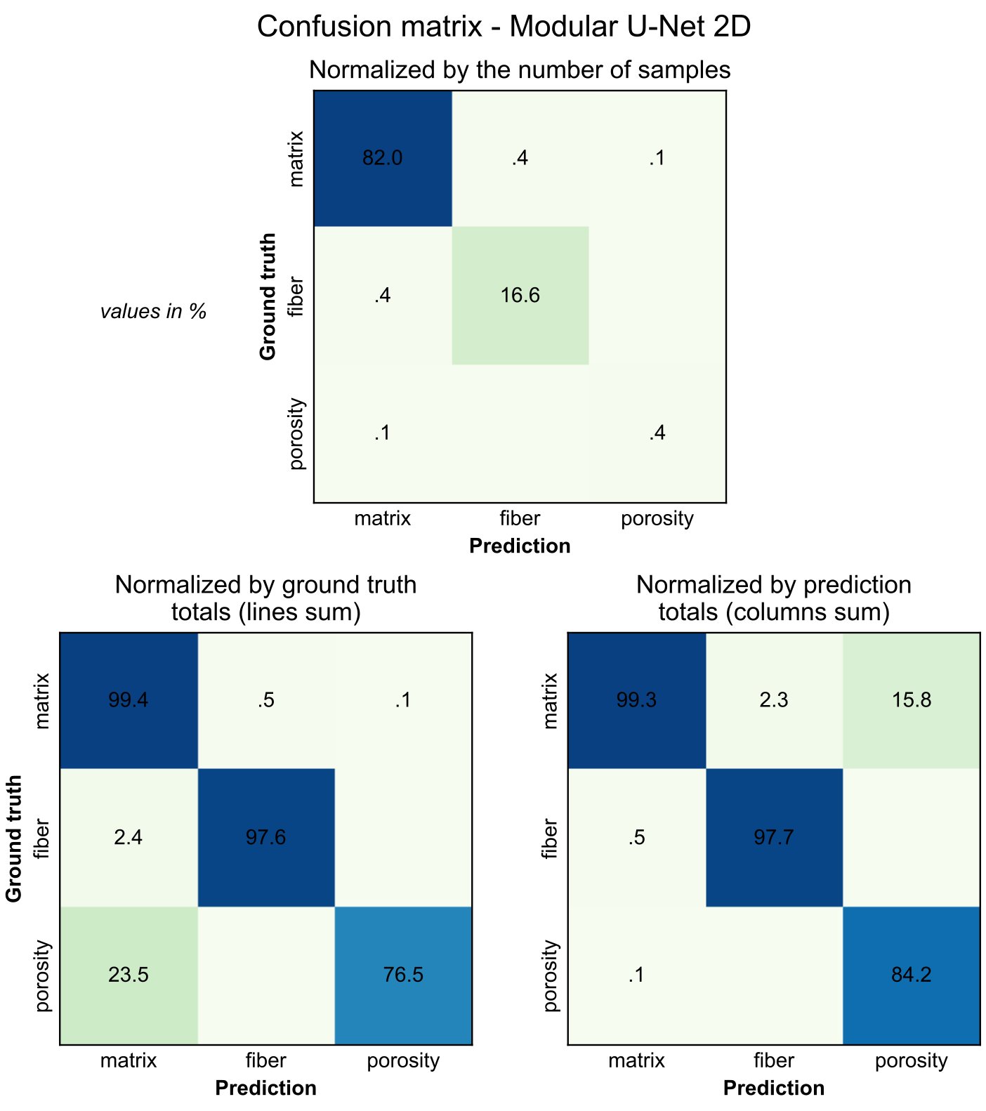
Figure 9 shows that, as the matrix and the fiber phases have high scores, the mean Jaccard index is driven by the performance on the porosity detection, which can also seen in Fig. 6. Recall that the baseline model Bin-ZeroOC is expected to have a Jaccard index of 35% on the porosity and 76.2% of mean (Table 4).

Figure 9: Class-wise Jaccard index Modular U-Net 2D, 2.5D, and 2D variations.

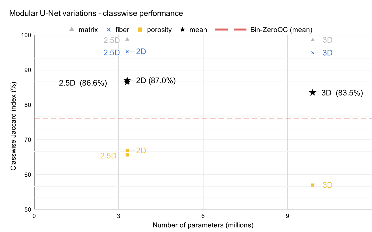
Figure 10 presents detailed confusion matrices. The top one is expressed percentage of the number of voxel counts. The two bottom ones are normalized, respectively, by row and column, and their diagonals correspond to the recall and the precision of each class.

Figure 10: Confusion matrices of the 2D model on the test set normalized in three different ways. (top) Normalized by the sum of all cells confounded. (bottom left) Normalized by the sum of ground truth labels (a.k.a. support) of each class (each line sums up to 100%); the diagonal corresponds to the recall values. (bottom right) Normalized by the sum of predicted labels of each class (each column sums up to 100%); the diagonal corresponds to the precision values.

References

- [1] Withers, P. J. et al. X-ray computed tomography. Nature Reviews Methods Primers 1, 1–21 (2021).
- [2] Maire, E. & Withers, P. Quantitative x-ray tomography. International Materials Reviews 59, 1–43 (2014).
- [3] Pacchioni, G. An upgrade to a bright future. Nature Reviews Physics 1, 100–101 (2019).
- [4] Shuai, S. et al. Fast synchrotron x-ray tomographic quantification of dendrite evolution during the solidification of mgsn alloys. Acta Materialia 118, 260–269 (2016).
- [5] Maire, E., Le Bourlot, C., Adrien, J., Mortensen, A. & Mokso, R. 20 hz x-ray tomography during an in situ tensile test. International Journal of Fracture 200, 3–12 (2016).
- [6] Shashank Kaira, C. et al. Automated correlative segmentation of large Transmission X-ray Microscopy (TXM) tomograms using deep learning. Materials Characterization 142, 203–210 (2018).
- [7] Strohmann, T. et al. Semantic segmentation of synchrotron tomography of multiphase Al-Si alloys using a convolutional neural network with a pixel-wise weighted loss function. Scientific Reports 9, 1–9 (2019).
- [8] Beucher, S. Watershed, Hierarchical Segmentation and Waterfall Algorithm. In Morphology and Its Applications to Image Processing, vol. 2, 69–76 (1994).
- [9] Beucher, C., S.and Lantuejoul. Use of Watersheds in Contour Detection.In International Workshop on Image Processing : Real-time Edge and Motion Detection/Estimation, Rennes, France. (1979).
- [10] F.Rosenblatt. The perceptron: a probabilistic model for information storage and organization in the brain. Psychological review 65 6, 386–408 (1958).
- [11] Bengio, Y., Y.and Lecun. Convolutional networks for images, speech, and time-series (1997).
- [12] Abadi, M. et al. TensorFlow: Large-scale machine learning on heterogeneous systems (2015). URL https://www.tensorflow.org/. Software available from tensorflow.org.
- [13] Long, J., Shelhamer, E. & Darrell, T. Fully Convolutional Networks for Semantic Segmentation. arXiv:1411.4038 [cs] (2015). URL http://arxiv.org/abs/1411.4038. ArXiv: 1411.4038.
- [14] Stan, T. & Thompson, P. W., Zachary T.and Voorhees. Optimizing convolutional neural networks to perform semantic segmentation on large materials imaging datasets: X-ray tomography and serial sectioning. Materials Characterization 160, 110119 (2020).
- [15] Badrinarayanan, V., Kendall, A. & Cipolla, R. SegNet: A Deep Convolutional Encoder-Decoder Architecture for Image Segmentation. IEEE Transactions on Pattern Analysis and Machine Intelligence 39, 2481–2495 (2017). URL 10.1109/TPAMI.2016.2644615. Conference Name: IEEE Transactions on Pattern Analysis and Machine Intelligence arxiv: 1511.00561.
- [16] Ronneberger, O., Fischer, P. & Brox, T. U-Net: Convolutional Networks for Biomedical Image Segmentation. arXiv:1505.04597 [cs] (2015). 1505.04597.
- [17] Çiçek, Ö., Abdulkadir, A., Lienkamp, T., S.and Brox & Ronneberger, O. 3D U-Net: Learning Dense Volumetric Segmentation from Sparse Annotation. In Medical Image Computing and Computer-Assisted Intervention (MICCAI) (2016).
- [18] Qin, X., Zhang, Z., Huang, C., Dehghan, M. & Zaiane, M., Osmar R.and Jagersand. U2-Net: Going Deeper with Nested U-Structure for Salient Object Detection. Pattern Recognition 106, 107404 (2020). 2005.09007.
- [19] Zhou, Z., Siddiquee, M. M. R., Tajbakhsh, N. & Liang, J. UNet++: A Nested U-Net Architecture for Medical Image Segmentation. arXiv:1807.10165 [cs, eess, stat] (2018). URL http://arxiv.org/abs/1807.10165. ArXiv: 1807.10165.
- [20] Oktay, O. et al. Attention U-Net: Learning Where to Look for the Pancreas. arXiv:1804.03999 [cs] (2018). 1804.03999.
- [21] Stoller, D., Ewert, S. & Dixon, S. Wave-U-Net: A Multi-Scale Neural Network for End-to-End Audio Source Separation. arXiv:1806.03185 [cs, eess, stat] (2018). 1806.03185.
- [22] Zhang, Z., Liu, Q. & Wang, Y. Road Extraction by Deep Residual U-Net. IEEE Geoscience and Remote Sensing Letters 15, 749–753 (2018).
- [23] Furat, O. et al. Machine Learning Techniques for the Segmentation of Tomographic Image Data of Functional Materials. Frontiers in Materials 6 (2019).
- [24] Schneider, C. A. & Rasband, K. W., Wayne S.and Eliceiri. NIH Image to ImageJ: 25 years of image analysis. Nature Methods 9, 671–675 (2012).
- [25] Schindelin, J. et al. Fiji: An open-source platform for biological-image analysis. Nature Methods 9, 676–682 (2012).
- [26] Bertoldo, J., Decencière, E., Ryckelynck, D. & Proudhon, H. Glass fiber-reinforced polyamide 66 3D X-ray computed tomography dataset for deep learning segmentation (2021). URL https://doi.org/10.5281/zenodo.4587827.
- [27] Mirone, A., Brun, E., Gouillart, E., Tafforeau, P. & Kieffer, J. The pyhst2 hybrid distributed code for high speed tomographic reconstruction with iterative reconstruction and a priori knowledge capabilities. Nuclear Instruments and Methods in Physics Research Section B: Beam Interactions with Materials and Atoms 324, 41–48 (2014). 1st International Conference on Tomography of Materials and Structures.
- [28] Paganin, D., Mayo, S. C., Gureyev, T. E., Miller, P. R. & Wilkins, S. W. Simultaneous phase and amplitude extraction from a single defocused image of a homogeneous object. Journal of Microscopy 206, 33–40 (2002).
- [29] Adams, L., R.and Bischof. Seeded region growing. IEEE Transactions on Pattern Analysis and Machine Intelligence 16, 641–647 (1994).
- [30] Bertoldo, J., Decencière, E., Ryckelynck, D. & Proudhon, H. Glass fiber-reinforced polyamide 66 3D X-ray computed tomography segmentation segmentation U-Nets (2021). URL https://doi.org/10.5281/zenodo.4601560.
- [31] Hanley, J. A. & McNeil, B. J. The meaning and use of the area under a receiver operating characteristic (ROC) curve. Radiology 143, 29–36 (1982).
- [32] Pouyanfar, S. et al. Dynamic Sampling in Convolutional Neural Networks for Imbalanced Data Classification. In 2018 IEEE Conference on Multimedia Information Processing and Retrieval (MIPR), 112–117 (2018).
- [33] Ando, S. & Huang, C. Y. Deep Over-sampling Framework for Classifying Imbalanced Data. In Ceci, M., Hollmén, J., Todorovski, L., Vens, C. & Džeroski, S. (eds.) Machine Learning and Knowledge Discovery in Databases, Lecture Notes in Computer Science, 770–785 (Springer International Publishing, Cham, 2017).
- [34] Cao, K., Wei, C., Gaidon, A., Arechiga, N. & Ma, T. Learning Imbalanced Datasets with Label-Distribution-Aware Margin Loss. arXiv:1906.07413 [cs, stat] (2019). 1906.07413.
- [35] Khan, S., Hayat, M., Zamir, W., Shen, J. & Shao, L. Striking the Right Balance with Uncertainty. arXiv:1901.07590 [cs] (2019). 1901.07590.
- [36] Yang, Y. & Xu, Z. Rethinking the Value of Labels for Improving Class-Imbalanced Learning. arXiv:2006.07529 [cs, stat] (2020). 2006.07529.
- [37] Liu, W., Wang, X. & Owens, Y., John D.and Li. Energy-based Out-of-distribution Detection. arXiv:2010.03759 [cs] (2020). 2010.03759.
- [38] Buades, A., Coll, B. & Morel, J.-M. Non-Local Means Denoising. Image Processing On Line 1, 208–212 (2011).
- [39] Darbon, J., Cunha, A., Chan, T., Osher, S. & Jensen, G. Fast nonlocal filtering applied to electron cryomicroscopy. In 2008 5th IEEE International Symposium on Biomedical Imaging: From Nano to Macro, 1331–1334 (2008).
- [40] European Organization For Nuclear Research & OpenAIRE. Zenodo (2013). URL https://www.zenodo.org/.
- [41] Duque-Arias, D. et al. On power Jaccard losses for semantic segmentation. In VISAPP 2021 : 16th International Conference on Computer Vision Theory and Applications (Vienne (on line), Austria, 2021).
- [42] Zhuang, J. et al. AdaBelief Optimizer: Adapting Stepsizes by the Belief in Observed Gradients. arXiv:2010.07468 [cs, stat] (2020). 2010.07468.
- [43] Kingma, J., Diederik P.and Ba. Adam: A Method for Stochastic Optimization. arXiv:1412.6980 [cs] (2017). 1412.6980.
- [44] Robbins, H. A stochastic approximation method. Annals of Mathematical Statistics 22, 400–407 (2007).
- [45] Chollet, F. et al. Keras. https://keras.io (2015).