AdaBelief Optimizer: Adapting Stepsizes by the Belief in Observed Gradients

Juntang Zhuang1; Tommy Tang2; Yifan Ding3; Sekhar Tatikonda1; Nicha Dvornek1;
Xenophon Papademetris1; James S. Duncan1
1
Yale University; 2 University of Illinois at Urbana-Champaign; 3 University of Central Florida
{j.zhuang;sekhar.tatikonda;nicha.dvornek;xenophon.papademetris;
james.duncan}@yale.edu; tommymt2@illinois.edu; yf.ding@knights.ucf.edu
Abstract

Most popular optimizers for deep learning can be broadly categorized as adaptive methods (e.g. Adam) and accelerated schemes (e.g. stochastic gradient descent (SGD) with momentum). For many models such as convolutional neural networks (CNNs), adaptive methods typically converge faster but generalize worse compared to SGD; for complex settings such as generative adversarial networks (GANs), adaptive methods are typically the default because of their stability. We propose AdaBelief to simultaneously achieve three goals: fast convergence as in adaptive methods, good generalization as in SGD, and training stability. The intuition for AdaBelief is to adapt the stepsize according to the "belief" in the current gradient direction. Viewing the exponential moving average (EMA) of the noisy gradient as the prediction of the gradient at the next time step, if the observed gradient greatly deviates from the prediction, we distrust the current observation and take a small step; if the observed gradient is close to the prediction, we trust it and take a large step. We validate AdaBelief in extensive experiments, showing that it outperforms other methods with fast convergence and high accuracy on image classification and language modeling. Specifically, on ImageNet, AdaBelief achieves comparable accuracy to SGD. Furthermore, in the training of a GAN on Cifar10, AdaBelief demonstrates high stability and improves the quality of generated samples compared to a well-tuned Adam optimizer. Code is available at https://github.com/juntang-zhuang/Adabelief-Optimizer

1 Introduction

Modern neural networks are typically trained with first-order gradient methods, which can be broadly categorized into two branches: the accelerated stochastic gradient descent (SGD) family [1], such as Nesterov accelerated gradient (NAG) [2], SGD with momentum [3] and heavy-ball method (HB) [4]; and the adaptive learning rate methods, such as Adagrad [5], AdaDelta [6], RMSProp [7] and Adam [8]. SGD methods use a global learning rate for all parameters, while adaptive methods compute an individual learning rate for each parameter.

Compared to the SGD family, adaptive methods typically converge fast in the early training phases, but have poor generalization performance [9, 10]. Recent progress tries to combine the benefits of both, such as switching from Adam to SGD either with a hard schedule as in SWATS [11], or with a smooth transition as in AdaBound [12]. Other modifications of Adam are also proposed: AMSGrad [13] fixes the error in convergence analysis of Adam, Yogi [14] considers the effect of minibatch size, MSVAG [15] dissects Adam as sign update and magnitude scaling, RAdam [16] rectifies the variance of learning rate, Fromage [17] controls the distance in the function space, and AdamW [18] decouples weight decay from gradient descent. Although these modifications achieve better accuracy compared to Adam, their generalization performance is typically worse than SGD on large-scale datasets such as ImageNet [19]; furthermore, compared with Adam, many optimizers are empirically unstable when training generative adversarial networks (GAN) [20].

To solve the problems above, we propose “AdaBelief”, which can be easily modified from Adam. Denote the observed gradient at step t𝑡t as gtsubscript𝑔𝑡g_{t} and its exponential moving average (EMA) as mtsubscript𝑚𝑡m_{t}. Denote the EMA of gt2superscriptsubscript𝑔𝑡2g_{t}^{2} and (gtmt)2superscriptsubscript𝑔𝑡subscript𝑚𝑡2(g_{t}-m_{t})^{2} as vtsubscript𝑣𝑡v_{t} and stsubscript𝑠𝑡s_{t}, respectively. mtsubscript𝑚𝑡m_{t} is divided by vtsubscript𝑣𝑡\sqrt{v_{t}} in Adam, while it is divided by stsubscript𝑠𝑡\sqrt{s_{t}} in AdaBelief. Intuitively, 1st1subscript𝑠𝑡\frac{1}{\sqrt{s_{t}}} is the “belief” in the observation: viewing mtsubscript𝑚𝑡m_{t} as the prediction of the gradient, if gtsubscript𝑔𝑡g_{t} deviates much from mtsubscript𝑚𝑡m_{t}, we have weak belief in gtsubscript𝑔𝑡g_{t}, and take a small step; if gtsubscript𝑔𝑡g_{t} is close to the prediction mtsubscript𝑚𝑡m_{t}, we have a strong belief in gtsubscript𝑔𝑡g_{t}, and take a large step. We validate the performance of AdaBelief with extensive experiments. Our contributions can be summarized as:

  • We propose AdaBelief, which can be easily modified from Adam without extra parameters. AdaBelief has three properties: (1) fast convergence as in adaptive gradient methods, (2) good generalization as in the SGD family, and (3) training stability in complex settings such as GAN.

  • We theoretically analyze the convergence property of AdaBelief in both convex optimization and non-convex stochastic optimization.

  • We validate the performance of AdaBelief with extensive experiments: AdaBelief achieves fast convergence as Adam and good generalization as SGD in image classification tasks on CIFAR and ImageNet; AdaBelief outperforms other methods in language modeling; in the training of a W-GAN [21], compared to a well-tuned Adam optimizer, AdaBelief significantly improves the quality of generated images, while several recent adaptive optimizers fail the training.

2 Methods

2.1 Details of AdaBelief Optimizer

Notations

By the convention in [8], we use the following notations:

  • f(θ),θdformulae-sequence𝑓𝜃𝜃superscript𝑑f(\theta)\in\mathbb{R},\theta\in\mathbb{R}^{d}: f𝑓f is the loss function to minimize, θ𝜃\theta is the parameter in dsuperscript𝑑\mathbb{R}^{d}

  • ,M(y)=argminxM1/2(xy)subscriptproduct𝑀𝑦subscriptargmin𝑥normsuperscript𝑀12𝑥𝑦\prod_{\mathcal{F},M}(y)=\mathrm{argmin}_{x\in\mathcal{F}}||M^{1/2}(x-y)||: projection of y𝑦y onto a convex feasible set \mathcal{F}

  • gtsubscript𝑔𝑡g_{t}: the gradient and step t𝑡t

  • mtsubscript𝑚𝑡m_{t}: exponential moving average (EMA) of gtsubscript𝑔𝑡g_{t}

  • vt,stsubscript𝑣𝑡subscript𝑠𝑡v_{t},s_{t}: vtsubscript𝑣𝑡v_{t} is the EMA of gt2superscriptsubscript𝑔𝑡2g_{t}^{2}, stsubscript𝑠𝑡s_{t} is the EMA of (gtmt)2superscriptsubscript𝑔𝑡subscript𝑚𝑡2(g_{t}-m_{t})^{2}

  • α,ϵ𝛼italic-ϵ\alpha,\epsilon: α𝛼\alpha is the learning rate, default is 103superscript10310^{-3}; ϵitalic-ϵ\epsilon is a small number, typically set as 108superscript10810^{-8}

  • β1,β2subscript𝛽1subscript𝛽2\beta_{1},\beta_{2}: smoothing parameters, typical values are β1=0.9,β2=0.999formulae-sequencesubscript𝛽10.9subscript𝛽20.999\beta_{1}=0.9,\beta_{2}=0.999

  • β1t,β2tsubscript𝛽1𝑡subscript𝛽2𝑡\beta_{1t},\beta_{2t} are the momentum for mtsubscript𝑚𝑡m_{t} and vtsubscript𝑣𝑡v_{t} respectively at step t𝑡t, and typically set as constant (e.g. β1t=β1,β2t=β2,t{1,2,T}formulae-sequencesubscript𝛽1𝑡subscript𝛽1formulae-sequencesubscript𝛽2𝑡subscript𝛽2for-all𝑡12𝑇\beta_{1t}=\beta_{1},\beta_{2t}=\beta_{2},\forall t\in\{1,2,...T\}

Initialize θ0subscript𝜃0\theta_{0}, m00subscript𝑚00m_{0}\leftarrow 0 , v00subscript𝑣00v_{0}\leftarrow 0, t0𝑡0t\leftarrow 0
While θtsubscript𝜃𝑡\theta_{t} not converged
        tt+1𝑡𝑡1t\leftarrow t+1
        gtθft(θt1)subscript𝑔𝑡subscript𝜃subscript𝑓𝑡subscript𝜃𝑡1g_{t}\leftarrow\nabla_{\theta}f_{t}(\theta_{t-1})
        mtβ1mt1+(1β1)gtsubscript𝑚𝑡subscript𝛽1subscript𝑚𝑡11subscript𝛽1subscript𝑔𝑡m_{t}\leftarrow\beta_{1}m_{t-1}+(1-\beta_{1})g_{t}
        vtβ2vt1+(1β2)gt2subscript𝑣𝑡subscript𝛽2subscript𝑣𝑡11subscript𝛽2superscriptsubscript𝑔𝑡2v_{t}\leftarrow\beta_{2}v_{t-1}+(1-\beta_{2})g_{t}^{2}
        Bias Correction
               mt^mt1β1t^subscript𝑚𝑡subscript𝑚𝑡1superscriptsubscript𝛽1𝑡\widehat{m_{t}}\leftarrow\frac{m_{t}}{1-\beta_{1}^{t}}, vt^vt1β2t^subscript𝑣𝑡subscript𝑣𝑡1superscriptsubscript𝛽2𝑡\widehat{v_{t}}\leftarrow\frac{v_{t}}{1-\beta_{2}^{t}}
        Update
               θt,vt^(θt1αmt^vt^+ϵ)subscript𝜃𝑡subscriptproduct^subscript𝑣𝑡subscript𝜃𝑡1𝛼^subscript𝑚𝑡^subscript𝑣𝑡italic-ϵ\theta_{t}\leftarrow\prod_{\mathcal{F},\sqrt{\widehat{v_{t}}}}\Big{(}\theta_{t-1}-\frac{\alpha\widehat{m_{t}}}{\sqrt{\widehat{v_{t}}}+\epsilon}\Big{)}
Algorithm 1 Adam Optimizer
Initialize θ0subscript𝜃0\theta_{0}, m00subscript𝑚00m_{0}\leftarrow 0 , s00subscript𝑠00s_{0}\leftarrow 0, t0𝑡0t\leftarrow 0
While θtsubscript𝜃𝑡\theta_{t} not converged
        tt+1𝑡𝑡1t\leftarrow t+1
        gtθft(θt1)subscript𝑔𝑡subscript𝜃subscript𝑓𝑡subscript𝜃𝑡1g_{t}\leftarrow\nabla_{\theta}f_{t}(\theta_{t-1})
        mtβ1mt1+(1β1)gtsubscript𝑚𝑡subscript𝛽1subscript𝑚𝑡11subscript𝛽1subscript𝑔𝑡m_{t}\leftarrow\beta_{1}m_{t-1}+(1-\beta_{1})g_{t}
        stβ2st1+(1β2)(gtmt)2+ϵsubscript𝑠𝑡subscript𝛽2subscript𝑠𝑡11subscript𝛽2superscriptsubscript𝑔𝑡subscript𝑚𝑡2italic-ϵs_{t}\leftarrow\beta_{2}s_{t-1}{+}(1{-}\beta_{2}){\color[rgb]{0,0,1}\definecolor[named]{pgfstrokecolor}{rgb}{0,0,1}(g_{t}{-}m_{t})^{2}{+}\epsilon}
        Bias Correction
               mt^mt1β1t^subscript𝑚𝑡subscript𝑚𝑡1superscriptsubscript𝛽1𝑡\widehat{m_{t}}\leftarrow\frac{m_{t}}{1-\beta_{1}^{t}}, st^st1β2t^subscript𝑠𝑡subscript𝑠𝑡1superscriptsubscript𝛽2𝑡\widehat{s_{t}}\leftarrow\frac{s_{t}}{1-\beta_{2}^{t}}
        Update
               θt,st^(θt1αmt^st^+ϵ)subscript𝜃𝑡subscriptproduct^subscript𝑠𝑡subscript𝜃𝑡1𝛼^subscript𝑚𝑡^subscript𝑠𝑡italic-ϵ\theta_{t}\leftarrow\prod_{\mathcal{F},\sqrt{\widehat{s_{t}}}}\Big{(}\theta_{t-1}-\frac{\alpha\widehat{m_{t}}}{\sqrt{{\color[rgb]{0,0,1}\definecolor[named]{pgfstrokecolor}{rgb}{0,0,1}\widehat{s_{t}}}}+{\color[rgb]{0,0,0}\definecolor[named]{pgfstrokecolor}{rgb}{0,0,0}\pgfsys@color@gray@stroke{0}\pgfsys@color@gray@fill{0}\epsilon}}\Big{)}
Algorithm  2 AdaBelief Optimizer
Comparison with Adam

Adam and AdaBelief are summarized in Algo. 1 and Algo. 2, where all operations are element-wise, with differences marked in blue. Note that no extra parameters are introduced in AdaBelief. Specifically, in Adam, the update direction is mt/vtsubscript𝑚𝑡subscript𝑣𝑡m_{t}/\sqrt{v_{t}}, where vtsubscript𝑣𝑡v_{t} is the EMA of gt2superscriptsubscript𝑔𝑡2g_{t}^{2}; in AdaBelief, the update direction is mt/stsubscript𝑚𝑡subscript𝑠𝑡m_{t}/\sqrt{s_{t}}, where stsubscript𝑠𝑡s_{t} is the EMA of (gtmt)2superscriptsubscript𝑔𝑡subscript𝑚𝑡2(g_{t}-m_{t})^{2}. Intuitively, viewing mtsubscript𝑚𝑡m_{t} as the prediction of gtsubscript𝑔𝑡g_{t}, AdaBelief takes a large step when observation gtsubscript𝑔𝑡g_{t} is close to prediction mtsubscript𝑚𝑡m_{t}, and a small step when the observation greatly deviates from the prediction. .^^.\widehat{.} represents bias-corrected value. Note that an extra ϵitalic-ϵ\epsilon is added to stsubscript𝑠𝑡s_{t} during bias-correction, in order to better match the assumption that stsubscript𝑠𝑡s_{t} is bouded below (the lower bound is at leat ϵitalic-ϵ\epsilon). For simplicity, we omit the bias correction step in theoretical analysis.

2.2 Intuitive explanation for benefits of AdaBelief

AdaBelief uses curvature information
Refer to caption
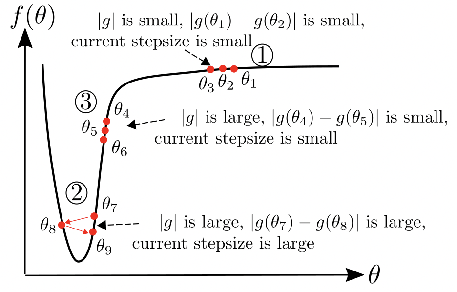
Figure 1: An ideal optimizer considers curvature of the loss function, instead of taking a large (small) step where the gradient is large (small) [22].

Update formulas for SGD, Adam and AdaBelief are:

ΔθtSGDΔsuperscriptsubscript𝜃𝑡𝑆𝐺𝐷\displaystyle\Delta\theta_{t}^{SGD} =αmt,ΔθtAdam=αmt/vt,formulae-sequenceabsent𝛼subscript𝑚𝑡Δsuperscriptsubscript𝜃𝑡𝐴𝑑𝑎𝑚𝛼subscript𝑚𝑡subscript𝑣𝑡\displaystyle=-\alpha m_{t},\ \ \Delta\theta_{t}^{Adam}=-\alpha m_{t}/\sqrt{v_{t}},
ΔθtAdaBeliefΔsuperscriptsubscript𝜃𝑡𝐴𝑑𝑎𝐵𝑒𝑙𝑖𝑒𝑓\displaystyle\Delta\theta_{t}^{AdaBelief} =αmt/stabsent𝛼subscript𝑚𝑡subscript𝑠𝑡\displaystyle=-\alpha m_{t}/\sqrt{s_{t}} (1)

Note that we name α𝛼\alpha as the “learning rate” and |Δθti|Δsuperscriptsubscript𝜃𝑡𝑖|\Delta\theta_{t}^{i}| as the “stepsize” for the i𝑖ith parameter. With a 1D example in Fig. 1, we demonstrate that AdaBelief uses the curvature of loss functions to improve training as summarized in Table 1, with a detailed description below:

Table 1: Comparison of optimizers in various cases in Fig. 1. “S” and “L” represent “small” and “large” stepsize, respectively. |Δθt|idealsubscriptΔsubscript𝜃𝑡𝑖𝑑𝑒𝑎𝑙|\Delta\theta_{t}|_{ideal} is the stepsize of an ideal optimizer. Note that only AdaBelief matches the behaviour of an ideal optimizer in all three cases.
Case 1 Case 2 Case 3
|gt|subscript𝑔𝑡|g_{t}|, vtsubscript𝑣𝑡v_{t} S L L
|gtgt1|subscript𝑔𝑡subscript𝑔𝑡1|g_{t}-g_{t-1}|, stsubscript𝑠𝑡s_{t} S L S
|Δθt|idealsubscriptΔsubscript𝜃𝑡𝑖𝑑𝑒𝑎𝑙|\Delta\theta_{t}|_{ideal} L S L
|Δθt|Δsubscript𝜃𝑡|\Delta\theta_{t}| SGD Adam AdaBelief SGD Adam AdaBelief SGD Adam AdaBelief
S L L L S S L S L

(1) In region 1g1 in Fig. 1, the loss function is flat, hence the gradient is close to 0. In this case, an ideal optimizer should take a large stepsize. The stepsize of SGD is proportional to the EMA of the gradient, hence is small in this case; while both Adam and AdaBelief take a large stepsize, because the denominator (vtsubscript𝑣𝑡\sqrt{v_{t}} and stsubscript𝑠𝑡\sqrt{s_{t}}) is a small value.

(2) In region 1g2, the algorithm oscillates in a “steep and narrow” valley, hence both |gt|subscript𝑔𝑡|g_{t}| and |gtgt1|subscript𝑔𝑡subscript𝑔𝑡1|g_{t}-g_{t-1}| is large. An ideal optimizer should decrease its stepsize, while SGD takes a large step (proportional to mtsubscript𝑚𝑡m_{t}). Adam and AdaBelief take a small step because the denominator (stsubscript𝑠𝑡\sqrt{s_{t}} and vtsubscript𝑣𝑡\sqrt{v_{t}}) is large.

(3) In region 1g3, we demonstrate AdaBelief’s advantage over Adam in the “large gradient, small curvature” case. In this case, |gt|subscript𝑔𝑡|g_{t}| and vtsubscript𝑣𝑡v_{t} are large, but |gtgt1|subscript𝑔𝑡subscript𝑔𝑡1|g_{t}-g_{t-1}| and stsubscript𝑠𝑡s_{t} are small; this could happen because of a small learning rate α𝛼\alpha. In this case, an ideal optimizer should increase its stepsize. SGD uses a large stepsize (α|gt|similar-toabsent𝛼subscript𝑔𝑡\sim\alpha|g_{t}|); in Adam, the denominator vtsubscript𝑣𝑡\sqrt{v_{t}} is large, hence the stepsize is small; in AdaBelief, denominator stsubscript𝑠𝑡\sqrt{s_{t}} is small, hence the stepsize is large as in an ideal optimizer.

To sum up, AdaBelief scales the update direction by the change in gradient, which is related to the Hessian. Therefore, AdaBelief considers curvature information and performs better than Adam.

AdaBelief considers the sign of gradient in denominator

We show the advantages of AdaBelief with a 2D example in this section, which gives us more intuition for high dimensional cases. In Fig. 2, we consider the loss function: f(x,y)=|x|+|y|𝑓𝑥𝑦𝑥𝑦f(x,y)=|x|+|y|. Note that in this simple problem, the gradient in each axis can only take {1,1}11\{1,-1\}. Suppose the start point is near the xlimit-from𝑥x-axis, e.g. y00,x00formulae-sequencesubscript𝑦00much-less-thansubscript𝑥00y_{0}\approx 0,x_{0}\ll 0. Optimizers will oscillate in the y𝑦y direction, and keep increasing in the x𝑥x direction.
Suppose the algorithm runs for a long time (t𝑡t is large), so the bias of EMA (β1t𝔼gtsuperscriptsubscript𝛽1𝑡𝔼subscript𝑔𝑡\beta_{1}^{t}\mathbb{E}g_{t}) is small:

mtsubscript𝑚𝑡\displaystyle m_{t} =EMA(g0,g1,gt)𝔼(gt),mt,x𝔼gt,x=1,mt,y𝔼gt,y=0formulae-sequenceabsent𝐸𝑀𝐴subscript𝑔0subscript𝑔1subscript𝑔𝑡𝔼subscript𝑔𝑡subscript𝑚𝑡𝑥𝔼subscript𝑔𝑡𝑥1subscript𝑚𝑡𝑦𝔼subscript𝑔𝑡𝑦0\displaystyle=EMA(g_{0},g_{1},...g_{t})\approx\mathbb{E}(g_{t}),\ \ m_{t,x}\approx\mathbb{E}g_{t,x}=1,\ \ m_{t,y}\approx\mathbb{E}g_{t,y}=0 (2)
vtsubscript𝑣𝑡\displaystyle v_{t} =EMA(g02,g12,gt2)𝔼(gt2),vt,x𝔼gt,x2=1,vt,y𝔼gt,y2=1.formulae-sequenceabsent𝐸𝑀𝐴superscriptsubscript𝑔02superscriptsubscript𝑔12superscriptsubscript𝑔𝑡2𝔼superscriptsubscript𝑔𝑡2subscript𝑣𝑡𝑥𝔼superscriptsubscript𝑔𝑡𝑥21subscript𝑣𝑡𝑦𝔼superscriptsubscript𝑔𝑡𝑦21\displaystyle=EMA(g_{0}^{2},g_{1}^{2},...g_{t}^{2})\approx\mathbb{E}(g_{t}^{2}),\ \ v_{t,x}\approx\mathbb{E}g_{t,x}^{2}=1,\ \ v_{t,y}\approx\mathbb{E}g_{t,y}^{2}=1. (3)
[Uncaptioned image]
Step 1 2 3 4 5
gxsubscript𝑔𝑥g_{x} 1 1 1 1 1
gysubscript𝑔𝑦g_{y} -1 1 -1 1 -1
Adam vxsubscript𝑣𝑥v_{x} 1 1 1 1 1
vysubscript𝑣𝑦v_{y} 1 1 1 1 1
AdaBelief sxsubscript𝑠𝑥s_{x} 0 0 0 0 0
sysubscript𝑠𝑦s_{y} 1 1 1 1 1
Figure 2: Left: Consider f(x,y)=|x|+|y|𝑓𝑥𝑦𝑥𝑦f(x,y)=|x|+|y|. Blue vectors represent the gradient, and the cross represents the optimal point. The optimizer oscillates in the y𝑦y direction, and keeps moving forward in the x𝑥x direction. Right: Optimization process for the example on the left. Note that denominator vt,x=vt,ysubscript𝑣𝑡𝑥subscript𝑣𝑡𝑦\sqrt{v_{t,x}}=\sqrt{v_{t,y}} for Adam, hence the same stepsize in x𝑥x and y𝑦y direction; while st,x<st,ysubscript𝑠𝑡𝑥subscript𝑠𝑡𝑦\sqrt{s_{t,x}}<\sqrt{s_{t,y}}, hence AdaBelief takes a large step in the x𝑥x direction, and a small step in the y𝑦y direction.

In practice, the bias correction step will further reduce the error between the EMA and its expectation if gtsubscript𝑔𝑡g_{t} is a stationary process [8]. Note that:

st=EMA((g0m0)2,(gtmt)2)𝔼[(gt𝔼gt)2]=𝐕𝐚𝐫gt,st,x0,st,y1formulae-sequencesubscript𝑠𝑡𝐸𝑀𝐴superscriptsubscript𝑔0subscript𝑚02superscriptsubscript𝑔𝑡subscript𝑚𝑡2𝔼delimited-[]superscriptsubscript𝑔𝑡𝔼subscript𝑔𝑡2𝐕𝐚𝐫subscript𝑔𝑡formulae-sequencesubscript𝑠𝑡𝑥0subscript𝑠𝑡𝑦1s_{t}=EMA\big{(}(g_{0}-m_{0})^{2},...(g_{t}-m_{t})^{2}\big{)}\approx\mathbb{E}\big{[}(g_{t}-\mathbb{E}g_{t})^{2}\big{]}=\mathbf{Var}g_{t},\ \ s_{t,x}\approx 0,\ \ s_{t,y}\approx 1

(4)

An example of the analysis above is summarized in Fig. 2. From Eq. 3 and Eq. 4, note that in Adam, vx=vysubscript𝑣𝑥subscript𝑣𝑦v_{x}=v_{y}; this is because the update of vtsubscript𝑣𝑡v_{t} only uses the amplitude of gtsubscript𝑔𝑡g_{t} and ignores its sign, hence the stepsize for the x𝑥x and y𝑦y direction is the same 1/vt,x=1/vt,y1subscript𝑣𝑡𝑥1subscript𝑣𝑡𝑦1/\sqrt{v_{t,x}}=1/\sqrt{v_{t,y}}. AdaBelief considers both the magnitude and sign of gtsubscript𝑔𝑡g_{t}, and 1/st,x1/st,ymuch-greater-than1subscript𝑠𝑡𝑥1subscript𝑠𝑡𝑦1/\sqrt{s_{t,x}}\gg 1/\sqrt{s_{t,y}}, hence takes a large step in the x𝑥x direction and a small step in the y𝑦y direction, which matches the behaviour of an ideal optimizer.

Update direction in Adam is close to “sign descent” in low-variance case

In this section, we demonstrate that when the gradient has low variance, the update direction in Adam is close to “sign descent”, hence deviates from the gradient. This is also mentioned in [15].

Under the following assumptions: (1) assume gtsubscript𝑔𝑡g_{t} is drawn from a stationary distribution, hence after bias correction, 𝔼vt=(𝔼gt)2+𝐕𝐚𝐫gt𝔼subscript𝑣𝑡superscript𝔼subscript𝑔𝑡2𝐕𝐚𝐫subscript𝑔𝑡\mathbb{E}v_{t}=(\mathbb{E}g_{t})^{2}+\mathbf{Var}g_{t}. (2) low-noise assumption, assume (𝔼gt)2𝐕𝐚𝐫gtmuch-greater-thansuperscript𝔼subscript𝑔𝑡2𝐕𝐚𝐫subscript𝑔𝑡(\mathbb{E}g_{t})^{2}\gg\mathbf{Var}g_{t}, hence we have 𝔼gt/𝔼vt𝔼gt/(𝔼gt)2=sign(𝔼gt)𝔼subscript𝑔𝑡𝔼subscript𝑣𝑡𝔼subscript𝑔𝑡superscript𝔼subscript𝑔𝑡2𝑠𝑖𝑔𝑛𝔼subscript𝑔𝑡\mathbb{E}g_{t}/\sqrt{\mathbb{E}v_{t}}\approx\mathbb{E}g_{t}/\sqrt{(\mathbb{E}g_{t})^{2}}=sign(\mathbb{E}g_{t}). (3) low-bias assumption, assume β1tsuperscriptsubscript𝛽1𝑡\beta_{1}^{t} (β1subscript𝛽1\beta_{1} to the power of t𝑡t) is small, hence mtsubscript𝑚𝑡m_{t} as an estimator of 𝔼gt𝔼subscript𝑔𝑡\mathbb{E}g_{t} has a small bias β1t𝔼gtsuperscriptsubscript𝛽1𝑡𝔼subscript𝑔𝑡\beta_{1}^{t}\mathbb{E}g_{t}. Then

ΔθtAdam=αmtvt+ϵα𝔼gt(𝔼gt)2+𝐕𝐚𝐫gt+ϵα𝔼gt𝔼gt=αsign(𝔼gt)Δsuperscriptsubscript𝜃𝑡𝐴𝑑𝑎𝑚𝛼subscript𝑚𝑡subscript𝑣𝑡italic-ϵ𝛼𝔼subscript𝑔𝑡superscript𝔼subscript𝑔𝑡2𝐕𝐚𝐫subscript𝑔𝑡italic-ϵ𝛼𝔼subscript𝑔𝑡norm𝔼subscript𝑔𝑡𝛼sign𝔼subscript𝑔𝑡\Delta\theta_{t}^{Adam}=-\alpha\frac{m_{t}}{\sqrt{v_{t}}+\epsilon}\approx-\alpha\frac{\mathbb{E}g_{t}}{\sqrt{(\mathbb{E}g_{t})^{2}+\mathbf{Var}g_{t}}+\epsilon}\approx-\alpha\frac{\mathbb{E}g_{t}}{||\mathbb{E}g_{t}||}=-\alpha\ \mathrm{sign}(\mathbb{E}g_{t})

(5)

In this case, Adam behaves like a “sign descent”; in 2D cases the update is ±45plus-or-minussuperscript45\pm 45^{\circ} to the axis, hence deviates from the true gradient direction. The “sign update” effect might cause the generalization gap between adaptive methods and SGD (e.g. on ImageNet) [23, 9]. For AdaBelief, when the variance of gtsubscript𝑔𝑡g_{t} is the same for all coordinates, the update direction matches the gradient direction; when the variance is not uniform, AdaBelief takes a small (large) step when the variance is large (small).
Refer to caption
((a)) loss function is
f(x,y)=|x|+|y|𝑓𝑥𝑦𝑥𝑦f(x,y)=|x|+|y|
Refer to caption
((b)) f(x,y)=|x+y|+|xy|𝑓𝑥𝑦𝑥𝑦𝑥𝑦f(x,y)=|x+y|+\\ |x-y| / 10
Refer to caption
((c)) f(x,y)=(x+y)2+(xy)2/10𝑓𝑥𝑦superscript𝑥𝑦2superscript𝑥𝑦210f(x,y)=(x+y)^{2}+(x-y)^{2}/10
Refer to caption
((d)) f(x,y)=|x|/10+|y|𝑓𝑥𝑦𝑥10𝑦f(x,y)=|x|/10+|y|
β1=β2=0.3subscript𝛽1subscript𝛽20.3\beta_{1}=\beta_{2}=0.3
Refer to caption
((e)) Trajectory for Beale function in 2D.
Refer to caption
((f)) Trajectory for Beale function in 3D.
Refer to caption
((g)) Trajectory for Rosenbrock function in 2D.
Refer to caption
((h)) Trajectory for Rosenbrock function in 3D.
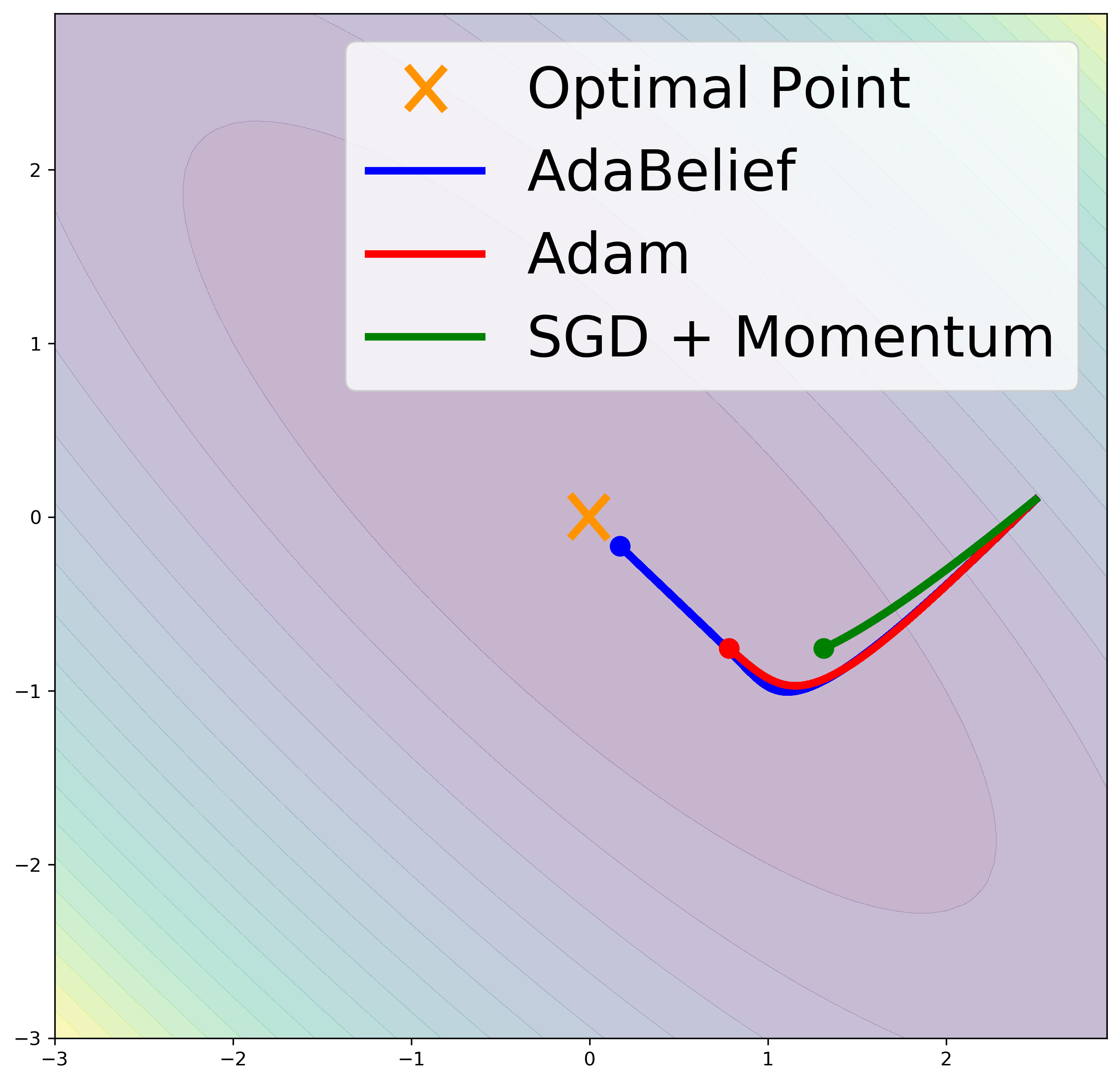
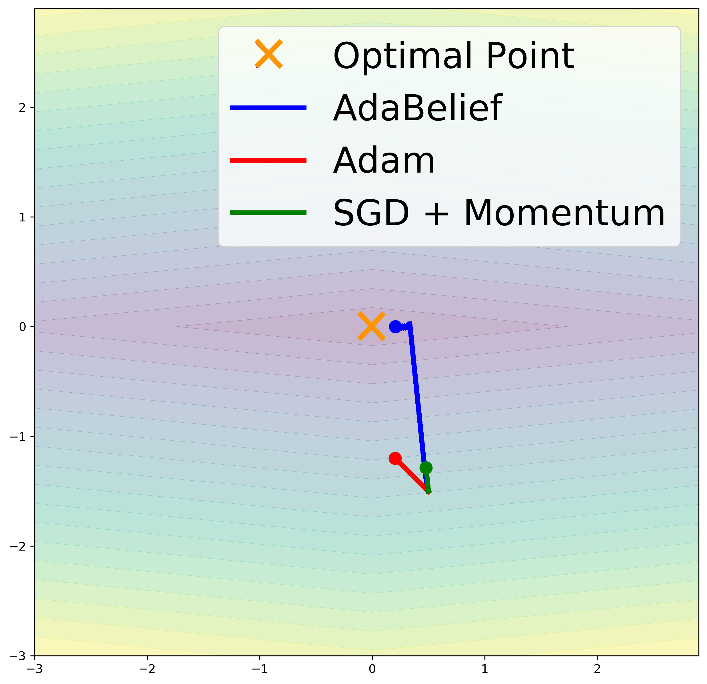
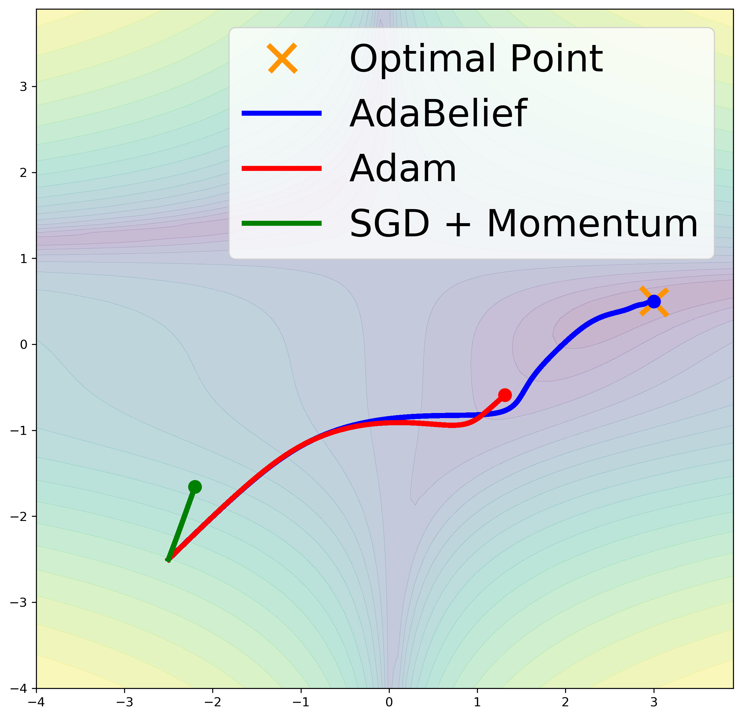
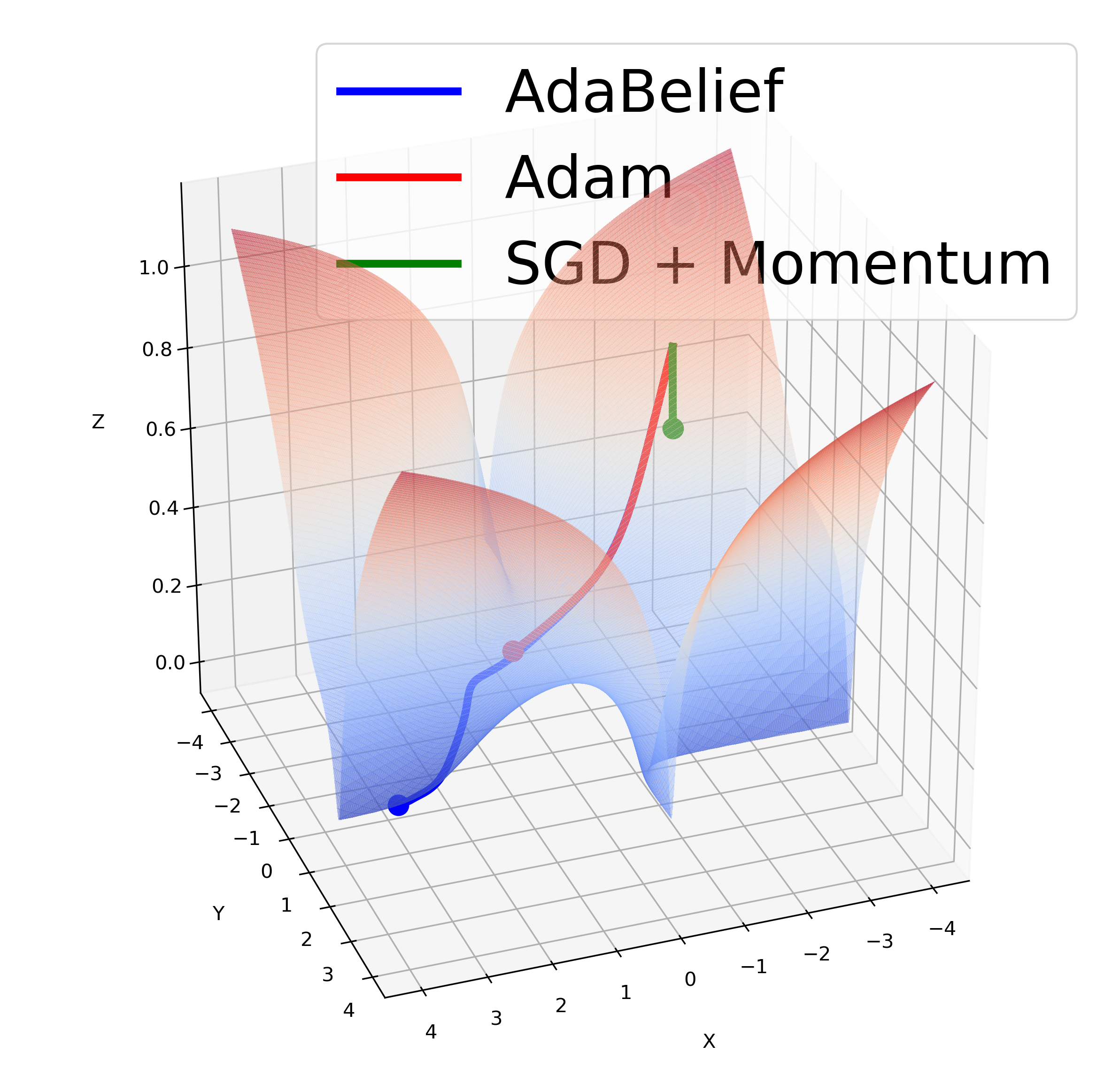
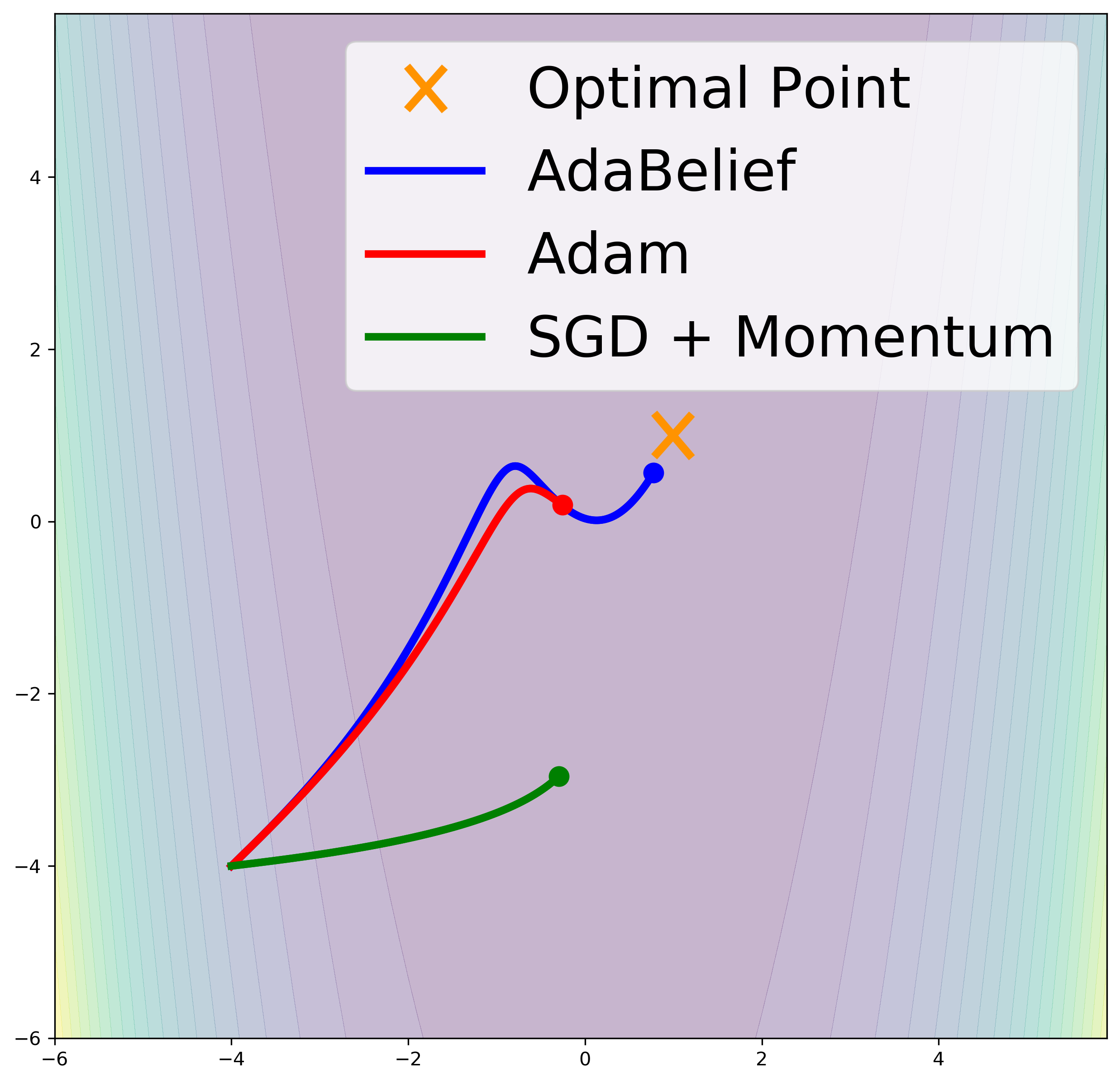
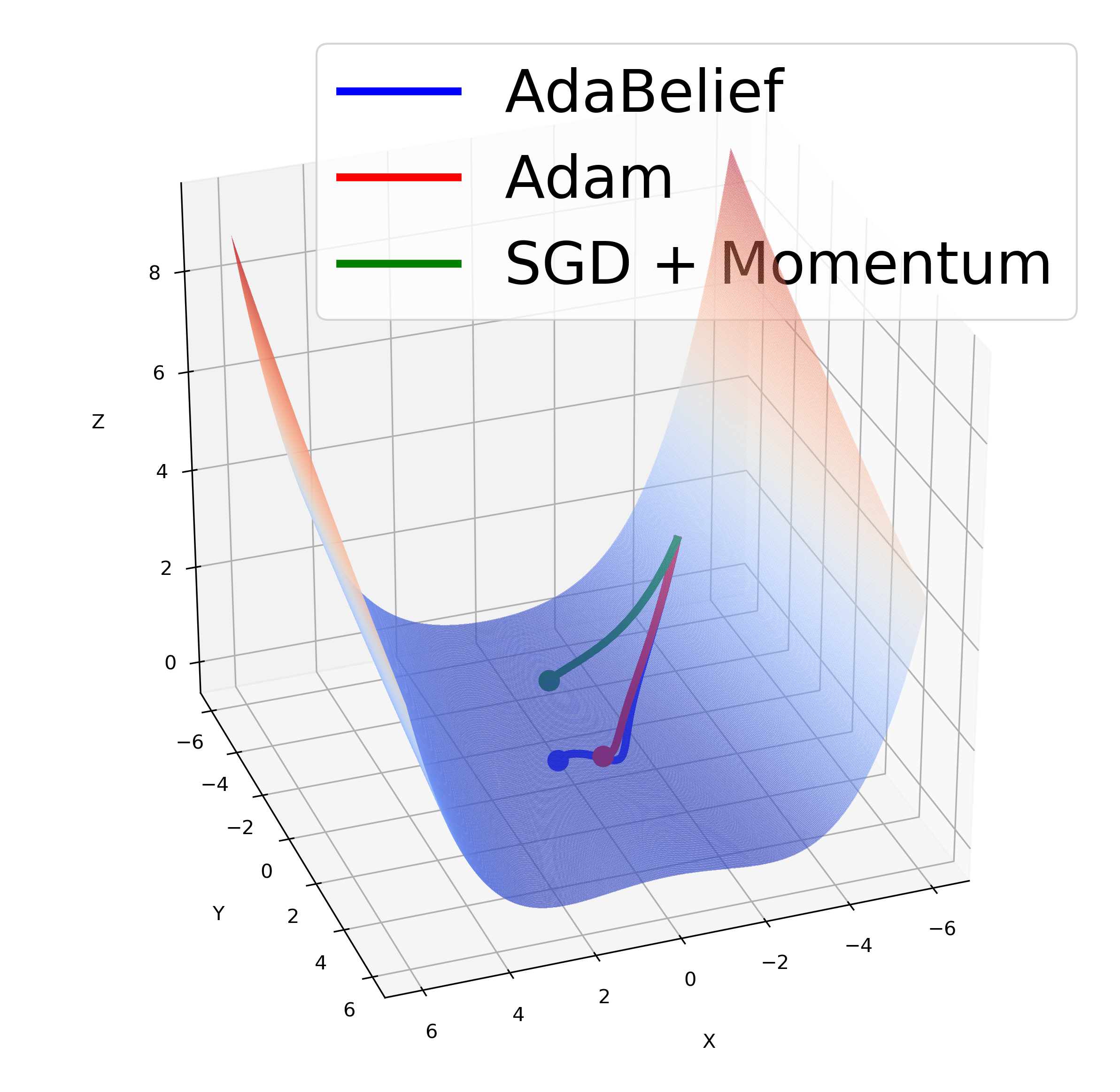
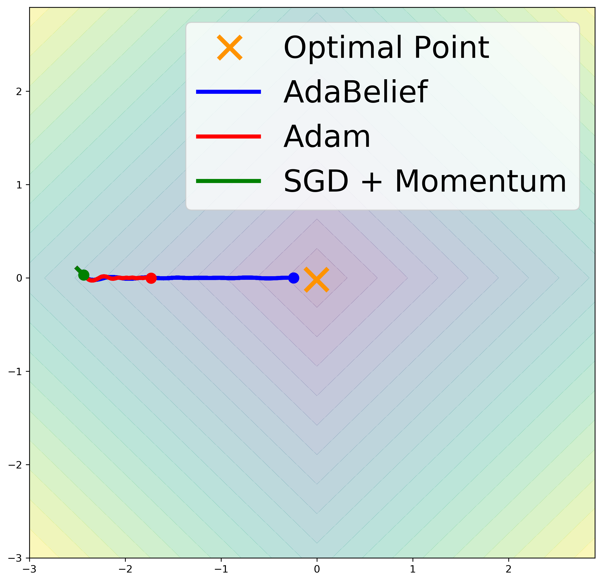
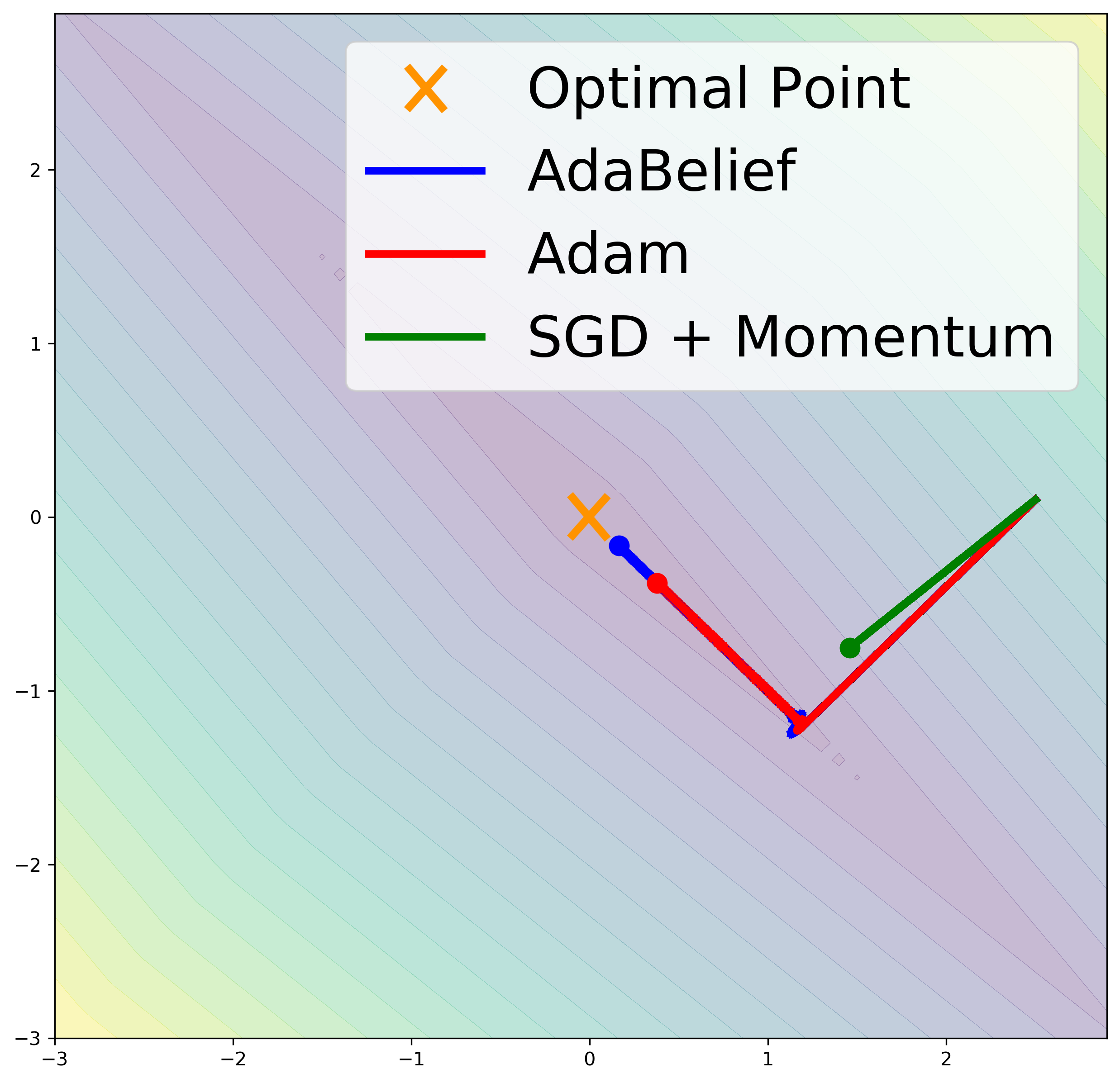
Figure 3: Trajectories of SGD, Adam and AdaBelief. AdaBelief reaches optimal point (marked as orange cross in 2D plots) the fastest in all cases. We refer readers to video examples.
Numerical experiments

In this section, we validate intuitions in Sec. 2.2. Examples are shown in Fig. 3, and we refer readers to more video examples111https://www.youtube.com/playlist?list=PL7KkG3n9bER6YmMLrKJ5wocjlvP7aWoOu for better visualization. In all examples, compared with SGD with momentum and Adam, AdaBelief reaches the optimal point at the fastest speed. Learning rate is α=103𝛼superscript103\alpha=10^{-3} for all optimizers. For all examples except Fig. 3(d), we set the parameters of AdaBelief to be the same as the default in Adam [8], β1=0.9,β2=0.999,ϵ=108formulae-sequencesubscript𝛽10.9formulae-sequencesubscript𝛽20.999italic-ϵsuperscript108\beta_{1}=0.9,\beta_{2}=0.999,\epsilon=10^{-8}, and set momentum as 0.9 for SGD. For Fig. 3(d), to match the assumption in Sec. 2.2, we set β1=β2=0.3subscript𝛽1subscript𝛽20.3\beta_{1}=\beta_{2}=0.3 for both Adam and AdaBelief, and set momentum as 0.30.30.3 for SGD.

  1. (a)

    Consider the loss function f(x,y)=|x|+|y|𝑓𝑥𝑦𝑥𝑦f(x,y)=|x|+|y| and a starting point near the x𝑥x axis. This setting corresponds to Fig. 2. Under the same setting, AdaBelief takes a large step in the x𝑥x direction, and a small step in the y𝑦y direction, validating our analysis. More examples such as f(x,y)=|x|/10+|y|𝑓𝑥𝑦𝑥10𝑦f(x,y)=|x|/10+|y| are in the supplementary videos.

  2. (b)

    For an inseparable L1subscript𝐿1L_{1} loss, AdaBelief outperforms other methods under the same setting.

  3. (c)

    For an inseparable L2subscript𝐿2L_{2} loss, AdaBelief outperforms other methods under the same setting.

  4. (d)

    We set β1=β2=0.3subscript𝛽1subscript𝛽20.3\beta_{1}=\beta_{2}=0.3 for Adam and AdaBelief, and set momentum as 0.30.30.3 in SGD. This corresponds to settings of Eq. 5. For the loss f(x,y)=|x|/10+|y|𝑓𝑥𝑦𝑥10𝑦f(x,y)=|x|/10+|y|, gtsubscript𝑔𝑡g_{t} is a constant for a large region, hence 𝔼gt𝐕𝐚𝐫gtmuch-greater-thannorm𝔼subscript𝑔𝑡𝐕𝐚𝐫subscript𝑔𝑡||\mathbb{E}g_{t}||\gg\mathbf{Var}g_{t}. As mentioned in [8], 𝔼mt=(1βt)𝔼gt𝔼subscript𝑚𝑡1superscript𝛽𝑡𝔼subscript𝑔𝑡\mathbb{E}m_{t}=(1-\beta^{t})\mathbb{E}g_{t}, hence a smaller β𝛽\beta decreases mt𝔼gtnormsubscript𝑚𝑡𝔼subscript𝑔𝑡||m_{t}-\mathbb{E}g_{t}|| faster to 0. Adam behaves like a sign descent (45superscript4545^{\circ} to the axis), while AdaBelief and SGD update in the direction of the gradient.

  5. (e)-(f)

    Optimization trajectory under default setting for the Beale [24] function in 2D and 3D.

  6. (g)-(h)

    Optimization trajectory under default setting for the Rosenbrock [25] function.

Above cases occur frequently in deep learning

Although the above cases are simple, they give hints to local behavior of optimizers in deep learning, and we expect them to occur frequently in deep learning. Hence, we expect AdaBelief to outperform Adam in general cases. Other works in the literature [13, 12] claim advantages over Adam, but are typically substantiated with carefully-constructed examples. Note that most deep networks use ReLU activation [26], which behaves like an absolute value function as in Fig. 3(a). Considering the interaction between neurons, most networks behave like case Fig. 3(b), and typically are ill-conditioned (the weight of some parameters are far larger than others) as in the figure. Considering a smooth loss function such as cross entropy or a smooth activation, this case is similar to Fig. 3(c). The case with Fig. 3(d) requires |mt||𝔼gt|𝐕𝐚𝐫gtsubscript𝑚𝑡𝔼subscript𝑔𝑡much-greater-than𝐕𝐚𝐫subscript𝑔𝑡|m_{t}|\approx|\mathbb{E}g_{t}|\gg\mathbf{Var}g_{t}, and this typically occurs at the late stages of training, where the learning rate α𝛼\alpha is decayed to a small value, and the network reaches a stable region.

2.3 Convergence analysis in convex and non-convex optimization

Similar to [13, 12, 27], for simplicity, we omit the de-biasing step (analysis applicable to de-biased version). Proof for convergence in convex and non-convex cases is in the appendix.

Optimization problem For deterministic problems, the problem to be optimized is minθf(θ)subscriptmin𝜃𝑓𝜃\mathrm{min}_{\theta\in\mathcal{F}}f(\theta); for online optimization, the problem is minθt=1Tft(θ)subscriptmin𝜃superscriptsubscript𝑡1𝑇subscript𝑓𝑡𝜃\mathrm{min}_{\theta\in\mathcal{F}}\sum_{t=1}^{T}f_{t}(\theta), where ftsubscript𝑓𝑡f_{t} can be interpreted as loss of the model with the chosen parameters in the t𝑡t-th step.

Theorem 2.1.

(Convergence in convex optimization) Let {θt}subscript𝜃𝑡\{\theta_{t}\} and {st}subscript𝑠𝑡\{s_{t}\} be the sequence obtained by AdaBelief, let 0β2<1,αt=αtformulae-sequence0subscript𝛽21subscript𝛼𝑡𝛼𝑡0\leq\beta_{2}<1,\alpha_{t}=\frac{\alpha}{\sqrt{t}}, β11=β1subscript𝛽11subscript𝛽1\beta_{11}=\beta_{1}, 0β1tβ1<1,stst+1,t[T]formulae-sequence0subscript𝛽1𝑡subscript𝛽11formulae-sequencesubscript𝑠𝑡subscript𝑠𝑡1for-all𝑡delimited-[]𝑇0\leq\beta_{1t}\leq\beta_{1}<1,s_{t}\leq s_{t+1},\forall t\in[T]. Let θ𝜃\theta\in\mathcal{F}, where dsuperscript𝑑\mathcal{F}\subset\mathbb{R}^{d} is a convex feasible set with bounded diameter Dsubscript𝐷D_{\infty}. Assume f(θ)𝑓𝜃f(\theta) is a convex function and gtG/2subscriptnormsubscript𝑔𝑡subscript𝐺2||g_{t}||_{\infty}\leq G_{\infty}/2 (hence gtmtGsubscriptnormsubscript𝑔𝑡subscript𝑚𝑡subscript𝐺||g_{t}-m_{t}||_{\infty}\leq G_{\infty}) and st,ic>0,t[T],θformulae-sequencesubscript𝑠𝑡𝑖𝑐0formulae-sequencefor-all𝑡delimited-[]𝑇𝜃s_{t,i}\geq c>0,\forall t\in[T],\theta\in\mathcal{F}. Denote the optimal point as θsuperscript𝜃\theta^{*}. For θtsubscript𝜃𝑡\theta_{t} generated with AdaBelief, we have the following bound on the regret: t=1T[ft(θt)ft(θ)]D2T2α(1β1)i=1dsT,i1/2+(1+β1)α1+logT2c(1β1)3i=1dg1:T,i22+D22(1β1)t=1Ti=1dβ1tst,i1/2αtsuperscriptsubscript𝑡1𝑇delimited-[]subscript𝑓𝑡subscript𝜃𝑡subscript𝑓𝑡superscript𝜃superscriptsubscript𝐷2𝑇2𝛼1subscript𝛽1superscriptsubscript𝑖1𝑑superscriptsubscript𝑠𝑇𝑖121subscript𝛽1𝛼1𝑇2𝑐superscript1subscript𝛽13superscriptsubscript𝑖1𝑑subscriptnormsuperscriptsubscript𝑔:1𝑇𝑖22superscriptsubscript𝐷221subscript𝛽1superscriptsubscript𝑡1𝑇superscriptsubscript𝑖1𝑑subscript𝛽1𝑡superscriptsubscript𝑠𝑡𝑖12subscript𝛼𝑡\displaystyle\sum_{t=1}^{T}[f_{t}(\theta_{t})-f_{t}(\theta^{*})]\leq\frac{D_{\infty}^{2}\sqrt{T}}{2\alpha(1-\beta_{1})}\sum_{i=1}^{d}s_{T,i}^{1/2}+\frac{(1+\beta_{1})\alpha\sqrt{1+\log T}}{2\sqrt{c}(1-\beta_{1})^{3}}\sum_{i=1}^{d}\Big{|}\Big{|}g_{1:T,i}^{2}\Big{|}\Big{|}_{2}+\frac{D_{\infty}^{2}}{2(1-\beta_{1})}\sum_{t=1}^{T}\sum_{i=1}^{d}\frac{\beta_{1t}s_{t,i}^{1/2}}{\alpha_{t}}

Corollary 2.1.1.

Suppose β1,t=β1λt, 0<λ<1formulae-sequencesubscript𝛽1𝑡subscript𝛽1superscript𝜆𝑡 0𝜆1\beta_{1,t}=\beta_{1}\lambda^{t},\ \ 0<\lambda<1 in Theorem (2.1), then we have:

t=1T[ft(θt)ft(θ)]D2T2α(1β1)i=1dsT,i1/2+(1+β1)α1+logT2c(1β1)3i=1dg1:T,i22+D2β1G2(1β1)(1λ)2αsuperscriptsubscript𝑡1𝑇delimited-[]subscript𝑓𝑡subscript𝜃𝑡subscript𝑓𝑡superscript𝜃superscriptsubscript𝐷2𝑇2𝛼1subscript𝛽1superscriptsubscript𝑖1𝑑superscriptsubscript𝑠𝑇𝑖121subscript𝛽1𝛼1𝑇2𝑐superscript1subscript𝛽13superscriptsubscript𝑖1𝑑subscriptnormsuperscriptsubscript𝑔:1𝑇𝑖22superscriptsubscript𝐷2subscript𝛽1subscript𝐺21subscript𝛽1superscript1𝜆2𝛼\sum_{t=1}^{T}[f_{t}(\theta_{t})-f_{t}(\theta^{*})]\leq\frac{D_{\infty}^{2}\sqrt{T}}{2\alpha(1-\beta_{1})}\sum_{i=1}^{d}s_{T,i}^{1/2}+\frac{(1+\beta_{1})\alpha\sqrt{1+\log T}}{2\sqrt{c}(1-\beta_{1})^{3}}\sum_{i=1}^{d}\Big{|}\Big{|}g_{1:T,i}^{2}\Big{|}\Big{|}_{2}+\frac{D_{\infty}^{2}\beta_{1}G_{\infty}}{2(1-\beta_{1})(1-\lambda)^{2}\alpha}

For the convex case, Theorem 2.1 implies the regret of AdaBelief is upper bounded by O(T)𝑂𝑇O(\sqrt{T}). Conditions for Corollary 2.1.1 can be relaxed to β1,t=β1/tsubscript𝛽1𝑡subscript𝛽1𝑡\beta_{1,t}=\beta_{1}/t as in [13], which still generates O(T)𝑂𝑇O(\sqrt{T}) regret. Similar to Theorem 4.1 in [8] and corollary 1 in [13], where the term i=1dvT,i1/2superscriptsubscript𝑖1𝑑superscriptsubscript𝑣𝑇𝑖12\sum_{i=1}^{d}v_{T,i}^{1/2} exists, we have i=1dsT,i1/2superscriptsubscript𝑖1𝑑superscriptsubscript𝑠𝑇𝑖12\sum_{i=1}^{d}s_{T,i}^{1/2}. Without further assumption, i=1dsT,i1/2<dGsuperscriptsubscript𝑖1𝑑superscriptsubscript𝑠𝑇𝑖12𝑑subscript𝐺\sum_{i=1}^{d}s_{T,i}^{1/2}<dG_{\infty} since gtmt<Gsubscriptnormsubscript𝑔𝑡subscript𝑚𝑡subscript𝐺||g_{t}-m_{t}||_{\infty}<G_{\infty} as assumed in Theorem 2.1, and dG𝑑subscript𝐺dG_{\infty} is constant. The literature [8, 13, 5] exerts a stronger assumption that i=1dTvT,i1/2dGTmuch-less-thansuperscriptsubscript𝑖1𝑑𝑇superscriptsubscript𝑣𝑇𝑖12𝑑subscript𝐺𝑇\sum_{i=1}^{d}\sqrt{T}v_{T,i}^{1/2}\ll dG_{\infty}\sqrt{T}. Our assumption could be similar or weaker, because 𝔼st=Vargt𝔼gt2=𝔼vt𝔼subscript𝑠𝑡Varsubscript𝑔𝑡𝔼superscriptsubscript𝑔𝑡2𝔼subscript𝑣𝑡\mathbb{E}s_{t}=\mathrm{Var}g_{t}\leq\mathbb{E}g_{t}^{2}=\mathbb{E}v_{t}, then we get better regret than O(T)𝑂𝑇O(\sqrt{T}).

Theorem 2.2.

(Convergence for non-convex stochastic optimization) Under the assumptions:

  • f𝑓f is differentiable; f(x)f(y)Lxy,x,ynorm𝑓𝑥𝑓𝑦𝐿norm𝑥𝑦for-all𝑥𝑦||\nabla f(x)-\nabla f(y)||\leq L||x-y||,\ \forall x,y; f𝑓f is also lower bounded.

  • The noisy gradient is unbiased, and has independent noise, i.e.gt=f(θt)+ζt,𝔼ζt=0,ζtζj,t,j,tjformulae-sequence𝑖𝑒formulae-sequencesubscript𝑔𝑡𝑓subscript𝜃𝑡subscript𝜁𝑡formulae-sequence𝔼subscript𝜁𝑡0bottomsubscript𝜁𝑡subscript𝜁𝑗for-all𝑡formulae-sequence𝑗𝑡𝑗i.e.\ g_{t}=\nabla f(\theta_{t})+\zeta_{t},\mathbb{E}\zeta_{t}=0,\zeta_{t}\bot\zeta_{j},\ \forall t,j\in\mathbb{N},t\neq j.

  • At step t𝑡t, the algorithm can access a bounded noisy gradient, and the true gradient is also bounded. i.e.||f(θt)||H,||gt||H,t>1i.e.\ \ ||\nabla f(\theta_{t})||\leq H,\ ||g_{t}||\leq H,\ \ \forall t>1.

Assume minj[d](s1)jc>0\operatorname*{min}_{j\in[d]}(s_{1})_{j}\geq c>0, noise in gradient has bounded variance, Var(gt)=σt2σ2,stst+1,tformulae-sequenceVarsubscript𝑔𝑡superscriptsubscript𝜎𝑡2superscript𝜎2formulae-sequencesubscript𝑠𝑡subscript𝑠𝑡1for-all𝑡\mathrm{Var}(g_{t})=\sigma_{t}^{2}\leq\sigma^{2},s_{t}\leq s_{t+1},\forall t\in\mathbb{N}, then the proposed algorithm satisfies:

as in [27], C1,C2,C3subscript𝐶1subscript𝐶2subscript𝐶3C_{1},C_{2},C_{3} are constants independent of d𝑑d and T𝑇T, and C4subscript𝐶4C_{4} is a constant independent of T𝑇T.

Corollary 2.2.1.

If c>C1H𝑐subscript𝐶1𝐻c>C_{1}H and assumptions for Theorem 2.2 are satisfied, we have:

1Tt=1T𝔼[αt2f(θt)2]1T11HC1c[C1α2σ2c(1+logT)+C2dαc+C3dα2c+C4]1𝑇superscriptsubscript𝑡1𝑇𝔼delimited-[]superscriptsubscript𝛼𝑡2superscriptnorm𝑓subscript𝜃𝑡21𝑇11𝐻subscript𝐶1𝑐delimited-[]subscript𝐶1superscript𝛼2superscript𝜎2𝑐1𝑇subscript𝐶2𝑑𝛼𝑐subscript𝐶3𝑑superscript𝛼2𝑐subscript𝐶4\frac{1}{T}\sum_{t=1}^{T}\mathbb{E}\Big{[}\alpha_{t}^{2}\Big{|}\Big{|}\nabla f(\theta_{t})\Big{|}\Big{|}^{2}\Big{]}\leq\frac{1}{T}\frac{1}{\frac{1}{H}-\frac{C_{1}}{c}}\Big{[}\frac{C_{1}\alpha^{2}\sigma^{2}}{c}\big{(}1+\log T\big{)}+C_{2}\frac{d\alpha}{\sqrt{c}}+C_{3}\frac{d\alpha^{2}}{c}+C_{4}\Big{]}

Theorem 2.2 implies the convergence rate for AdaBelief in the non-convex case is O(logT/T)𝑂𝑇𝑇O(\log T/\sqrt{T}), which is similar to Adam-type optimizers [13, 27]. Note that regret bounds are derived in the worst possible case, while empirically AdaBelief outperforms Adam mainly because the cases in Sec. 2.2 occur more frequently. It is possible that the above bounds are loose. Also note that we assume stst+1subscript𝑠𝑡subscript𝑠𝑡1s_{t}{\leq}s_{t+1}, in code this requires to use element wise maximum between stsubscript𝑠𝑡s_{t} and st+1subscript𝑠𝑡1s_{t+1} in the denominator.

Refer to caption
((a)) VGG11 on Cifar10
Refer to caption
((b)) ResNet34 on Cifar10
Refer to caption
((c)) DenseNet121 on Cifar10
Refer to caption
((d)) VGG11 on Cifar100
Refer to caption
((e)) ResNet34 on Cifar100
Refer to caption
((f)) DenseNet121 on Cifar100
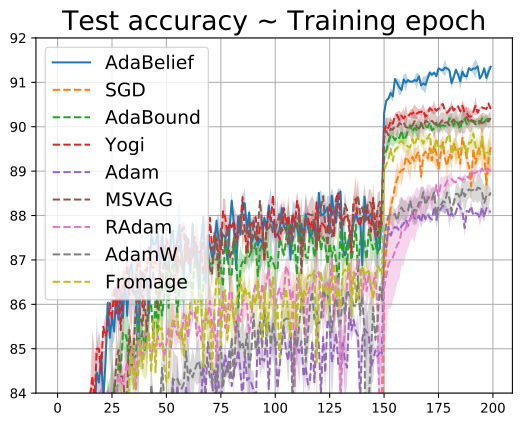
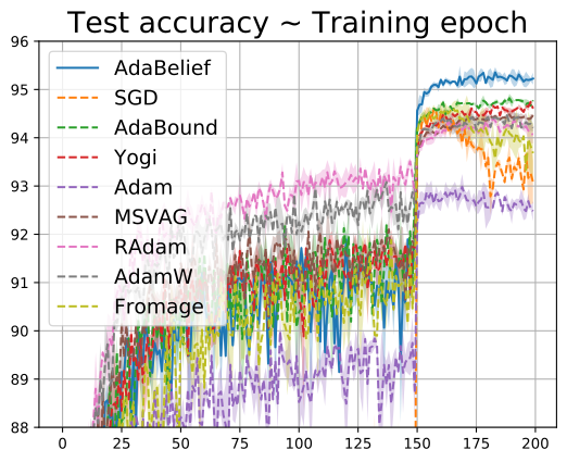
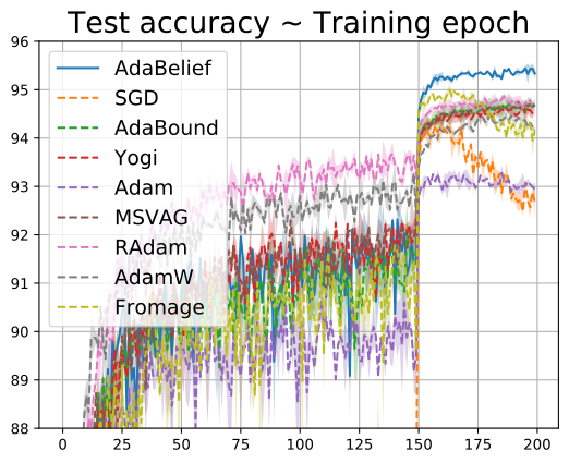
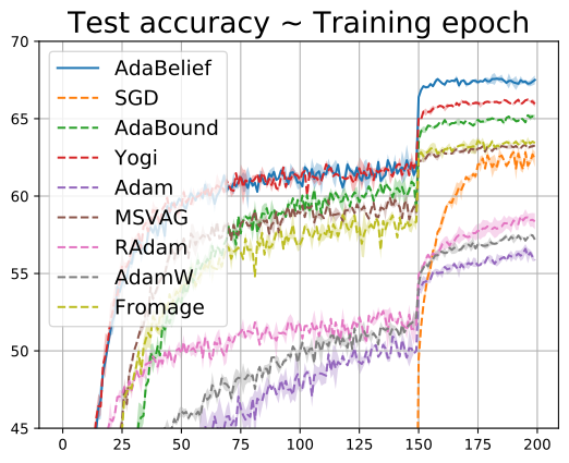
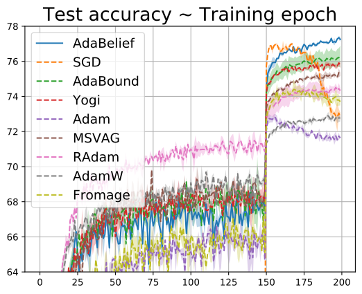
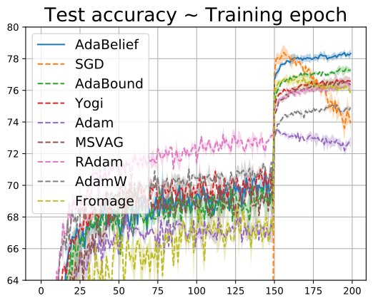
Figure 4: Test accuracy ([μ±σ]delimited-[]plus-or-minus𝜇𝜎[\mu\pm\sigma]) on Cifar. Code modified from official implementation of AdaBound.

3 Experiments

We performed extensive comparisons with other optimizers, including SGD [3], AdaBound [12], Yogi [14], Adam [8], MSVAG [15], RAdam [16], Fromage [17] and AdamW [18]. The experiments include: (a) image classification on Cifar dataset [28] with VGG [29], ResNet [30] and DenseNet [31], and image recognition with ResNet on ImageNet [32]; (b) language modeling with LSTM [33] on Penn TreeBank dataset [34]; (c) wasserstein-GAN (WGAN) [21] on Cifar10 dataset. We emphasize (c) because prior work focuses on convergence and accuracy, yet neglects training stability.

Hyperparameter tuning

We performed a careful hyperparameter tuning in experiments. On image classification and language modeling we use the following:

Table 2: Top-1 accuracy of ResNet18 on ImageNet. {\dagger} is reported in [35], {\ddagger} is reported in [16]
AdaBelief SGD AdaBound Yogi Adam MSVAG RAdam AdamW
70.08 70.23 68.13 68.23 63.79 (66.54) 65.99 67.62 67.93

\bullet AdaBelief:    We use the default parameters of Adam: β1=0.9,β2=0.999,ϵ=108,α=103formulae-sequencesubscript𝛽10.9formulae-sequencesubscript𝛽20.999formulae-sequenceitalic-ϵsuperscript108𝛼superscript103\beta_{1}=0.9,\beta_{2}=0.999,\epsilon=10^{-8},\alpha=10^{-3}.
\bullet SGD, Fromage:    We set the momentum as 0.90.90.9, which is the default for many networks such as ResNet [30] and DenseNet[31]. We search learning rate among {10.0,1.0,0.1,0.01,0.001}10.01.00.10.010.001\{10.0,1.0,0.1,0.01,0.001\}.
\bullet Adam, Yogi, RAdam, MSVAG, AdaBound:  We search for optimal β1subscript𝛽1\beta_{1} among {0.5,0.6,0.7,0.8,0.9}0.50.60.70.80.9\{0.5,0.6,0.7,0.8,0.9\}, search for α𝛼\alpha as in SGD, and set other parameters as their own default values in the literature.
\bullet AdamW:    We use the same parameter searching scheme as Adam. For other optimizers, we set the weight decay as 5×1045superscript1045\times 10^{-4}; for AdamW, since the optimal weight decay is typically larger [18], we search weight decay among {104,5×104,103,102}superscript1045superscript104superscript103superscript102\{10^{-4},5\times 10^{-4},10^{-3},10^{-2}\}.
For the training of a GAN, we set β1=0.5,ϵ=1012formulae-sequencesubscript𝛽10.5italic-ϵsuperscript1012\beta_{1}=0.5,\epsilon=10^{-12} for AdaBelief in a small GAN with vanilla CNN generator, and use ϵ=1016italic-ϵsuperscript1016\epsilon=10^{-16} for a larger spectral normalization GAN (SN-GAN) with a ResNet generator; for other methods, we search for β1subscript𝛽1\beta_{1} among {0.5,0.6,0.7,0.8,0.9}0.50.60.70.80.9\{0.5,0.6,0.7,0.8,0.9\}, and search for ϵitalic-ϵ\epsilon among {103,105,108,1010,1012}superscript103superscript105superscript108superscript1010superscript1012\{10^{-3},10^{-5},10^{-8},10^{-10},10^{-12}\}. We set learning rate as 2×1042superscript1042\times 10^{-4} for all methods. Note that the recommended parameters for Adam [36] and for RMSProp [37] are within the search range.
Refer to caption
Refer to caption
Refer to caption
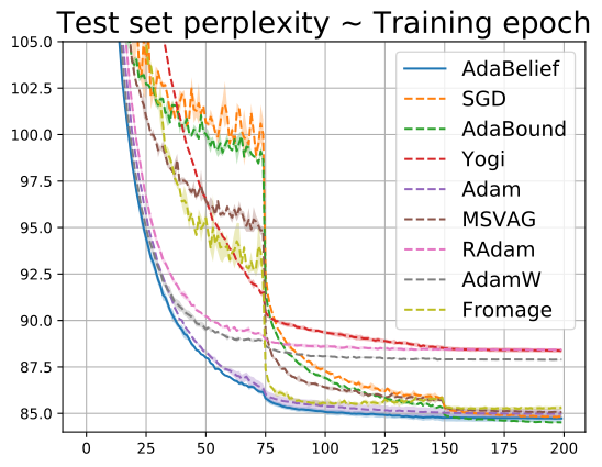
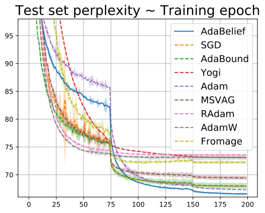
Figure 5: Left to right: perplexity ([μ±σ]delimited-[]plus-or-minus𝜇𝜎[\mu\pm\sigma]) on Penn Treebank for 1,2,3-layer LSTM. Lower is better.
Refer to caption
Refer to caption
((a)) FID score of WGAN.
Refer to caption
Refer to caption
((b)) FID score of WGAN-GP.
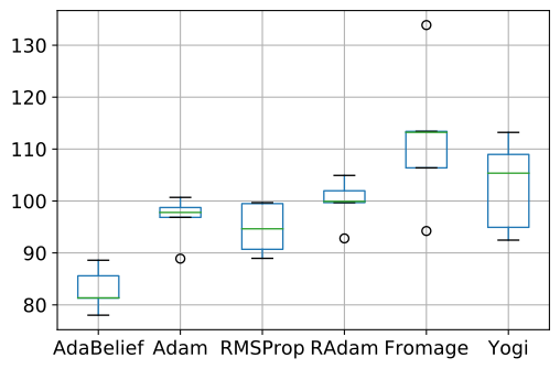
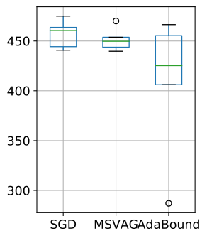
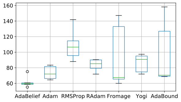
Figure 6: FID score of WGAN and WGAN-GP using a vanilla CNN generator on Cifar10. Lower is better. For each model, successful and failed optimizers are shown in the left and right respectively, with different ranges in y value.
CNNs on image classification

We experiment with VGG11, ResNet34 and DenseNet121 on Cifar10 and Cifar100 dataset. We use the official implementation of AdaBound, hence achieved an exact replication of [12]. For each optimizer, we search for the optimal hyperparameters, and report the mean and standard deviation of test-set accuracy (under optimal hyperparameters) for 3 runs with random initialization. As Fig. 4 shows, AdaBelief achieves fast convergence as in adaptive methods such as Adam while achieving better accuracy than SGD and other methods.

We then train a ResNet18 on ImageNet, and report the accuracy on the validation set in Table 2. Due to the heavy computational burden, we could not perform an extensive hyperparameter search; instead, we report the result of AdaBelief with the default parameters of Adam (β1=0.9,β2=0.999,ϵ=108formulae-sequencesubscript𝛽10.9formulae-sequencesubscript𝛽20.999italic-ϵsuperscript108\beta_{1}=0.9,\beta_{2}=0.999,\epsilon=10^{-8}) and decoupled weight decay as in [16, 18]; for other optimizers, we report the best result in the literature. AdaBelief outperforms other adaptive methods and achieves comparable accuracy to SGD (70.08 v.s. 70.23), which closes the generalization gap between adaptive methods and SGD. Experiments validate the fast convergence and good generalization performance of AdaBelief.

LSTM on language modeling

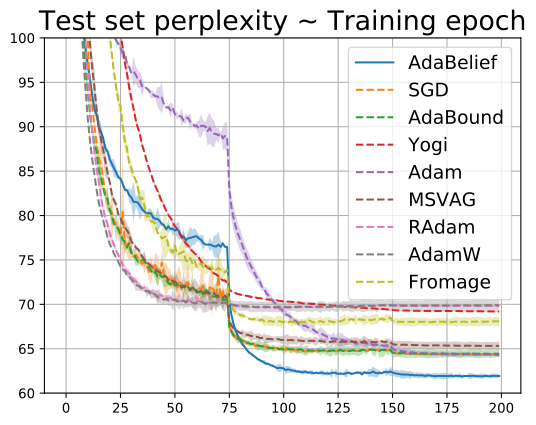
We experiment with LSTM on the Penn TreeBank dataset [34], and report the perplexity (lower is better) on the test set in Fig. 5. We report the mean and standard deviation across 3 runs. For both 2-layer and 3-layer LSTM models, AdaBelief achieves the lowest perplexity, validating its fast convergence as in adaptive methods and good accuracy. For the 1-layer model, the performance of AdaBelief is close to other optimizers.
Refer to caption
Refer to caption
Refer to caption
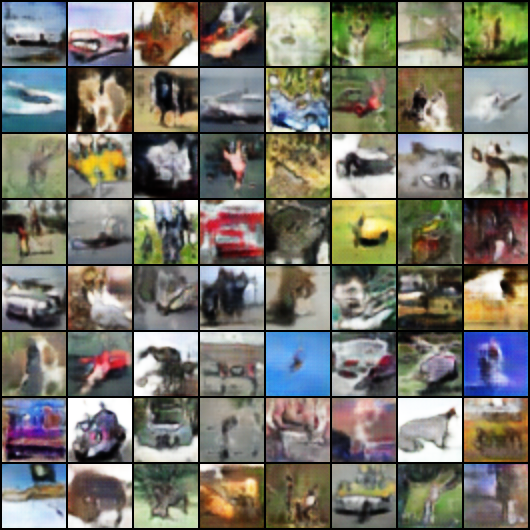
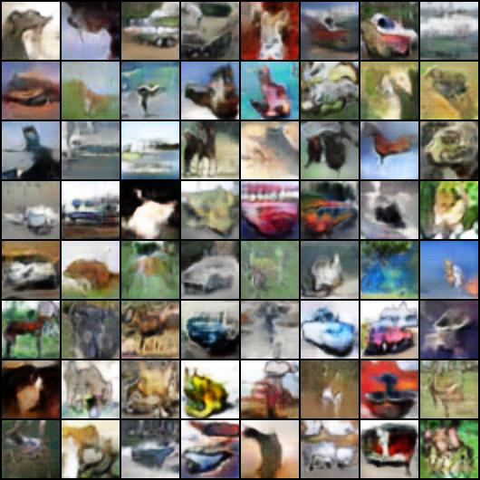
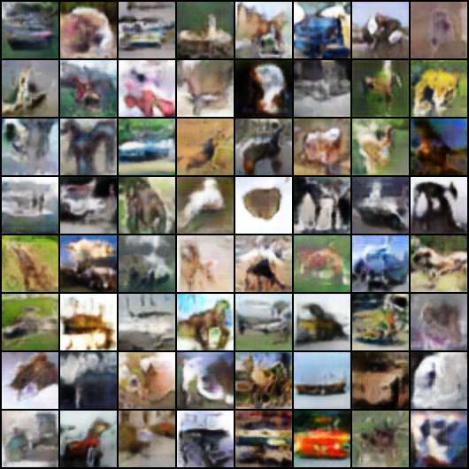
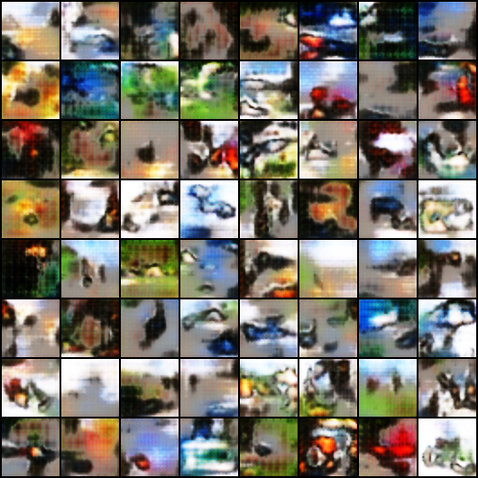
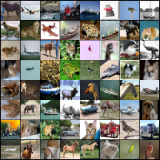
Figure 7: Left to right: real images, samples from WGAN, WGAN-GP (both trained by AdaBelief).
Table 3: FID (lower is better) of a SN-GAN with ResNet generator on Cifar10.
AdaBelief RAdam RMSProp Adam Fromage Yogi SGD MSVAG AdaBound
12.52±0.16plus-or-minus12.520.16\mathbf{12.52\pm 0.16} 12.70±0.12plus-or-minus12.700.1212.70\pm 0.12 13.13±0.12plus-or-minus13.130.1213.13\pm 0.12 13.05±0.19plus-or-minus13.050.1913.05\pm 0.19 42.75±0.15plus-or-minus42.750.1542.75\pm 0.15 14.25±0.15plus-or-minus14.250.1514.25\pm 0.15 49.70±0.41plus-or-minus49.700.4149.70\pm 0.41 48.35±5.44plus-or-minus48.355.4448.35\pm 5.44 55.65±2.15plus-or-minus55.652.1555.65\pm 2.15
Table 4: Comparison of AdaBelief and Padam. Higher Acc (lower FID) is better. {\ddagger} is from [35].
AdaBelief Padam
p=1/2 (Adam) p=2/5 p=1/4 p=1/5 p=1/8 p=1/16 p = 0 (SGD)
ImageNet Acc 70.08 63.79{\ddagger} - - - 70.07{\ddagger} - 70.23 {\ddagger}
FID (WGAN) 83.0±plus-or-minus\pm 4.1 96.6±plus-or-minus\pm4.5 97.5±plus-or-minus\pm2.8 426.4±plus-or-minus\pm49.6 401.5±plus-or-minus\pm33.2 328.1±plus-or-minus\pm37.2 362.6±plus-or-minus\pm43.9 469.3 ±plus-or-minus\pm 7.9
FID (WGAN-GP) 61.8±plus-or-minus\pm 7.7 73.5±plus-or-minus\pm8.7 87.1±plus-or-minus\pm6.0 155.1±plus-or-minus\pm23.8 167.3±plus-or-minus\pm27.6 203.6±plus-or-minus\pm18.9 228.5±plus-or-minus\pm25.8 244.3±plus-or-minus\pm 27.4
Table 5: BLEU score (higher is better) on IWSL14 task.
Adam RAdam AdaHessian AdaBelief
35.60 35.51 35.90 35.85
Table 6: mAP (higher is better) on PASCAL VOC object detection
Adam RAdam SGD AdaBelief
71.47 76.58 79.50 81.02
Generative adversarial networks

Stability of optimizers is important in practice such as training of GANs, yet recently proposed optimizers often lack experimental validations. The training of a GAN alternates between generator and discriminator in a mini-max game, and is typically unstable [20]; SGD often generates mode collapse, and adaptive methods such as Adam and RMSProp are recommended in practice [38, 37, 39]. Therefore, training of GANs is a good test for the stability.

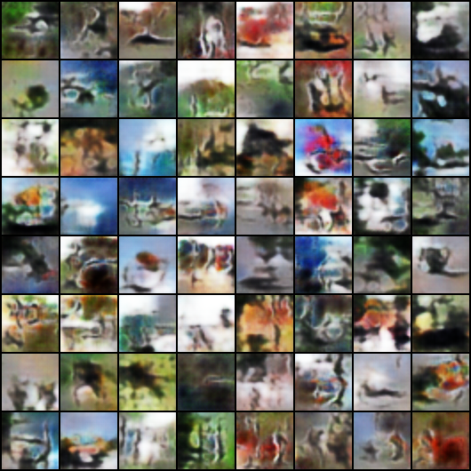
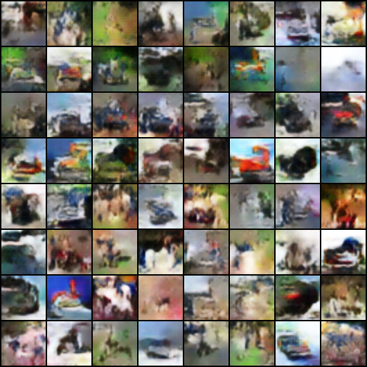
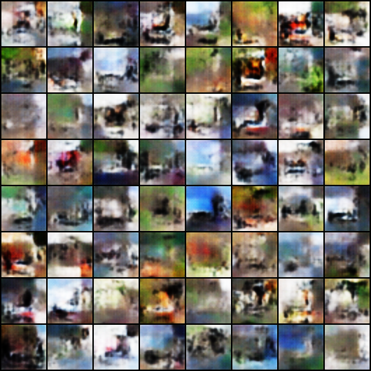
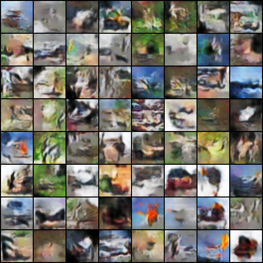
We experiment with one of the most widely used models, the Wasserstein-GAN (WGAN) [21] and the improved version with gradient penalty (WGAN-GP) [37] using a small model with vanilla CNN generator. Using each optimizer, we train the model for 100 epochs, generate 64,000 fake images from noise, and compute the Frechet Inception Distance (FID) [40] between the fake images and real dataset (60,000 real images). FID score captures both the quality and diversity of generated images and is widely used to assess generative models (lower FID is better). For each optimizer, under its optimal hyperparameter settings, we perform 5 runs of experiments, and report the results in Fig. 6 and Fig. 7. AdaBelief significantly outperforms other optimizers, and achieves the lowest FID score.

Besides the small model above, we also experiment with a large model using a ResNet generator and spectral normalization in the discriminator (SN-GAN). Results are summarized in Table. 3. Compared with a vanilla GAN, all FID scores are lower because the SN-GAN is more advanced. Compared with other optimizers, AdaBelief achieves the lowest FID with both large and small GANs.

Remarks

Recent research on optimizers tries to combine the fast convergence of adaptive methods with high accuracy of SGD. AdaBound [12] achieves this goal on Cifar, yet its performance on ImageNet is still inferior to SGD [35]. Padam [35] closes this generalization gap on ImageNet; writing the update as θt+1=θtαmt/vtpsubscript𝜃𝑡1subscript𝜃𝑡𝛼subscript𝑚𝑡superscriptsubscript𝑣𝑡𝑝\theta_{t+1}=\theta_{t}-\alpha m_{t}/v_{t}^{p}, SGD sets p=0𝑝0p=0, Adam sets p=0.5𝑝0.5p=0.5, and Padam searches p𝑝p between 0 and 0.5 (outside this region Padam diverges [35, 41]). Intuitively, compared to Adam, by using a smaller p𝑝p, Padam sacrifices the adaptivity for better generalization as in SGD; however, without good adaptivity, Padam loses training stability. As in Table 4, compared with Padam, AdaBelief achieves a much lower FID score in the training of GAN, meanwhile achieving slightly higher accuracy on ImageNet classification. Furthermore, AdaBelief has the same number of parameters as Adam, while Padam has one more parameter hence is harder to tune.

3.1 Extra experiments

We conducted extra experiments according to public discussions after publication. Considering the heavy computation burden, we did not compare Adabelief with all other optimizers as in previous sections, instead we only compare with the result from the official implementations. For details and code to reproduce results, please refer to our github page.

Neural machine translation with Transformer

We conducted experiments with a Transformer model [42]. The code is modified from the official implementation of AdaHessian [43]. As shown in Table. 5, AdaBelief outperforms Adam and RAdam. AdaBelief is slightly worse than AdaHessian, this could be caused by the "block-averaging" trick in AdaHessian, which could be used in AdaBelief but requires extra coding efforts.

Object detection

We show the results on PASCAL VOC object deetection with a Faster-RCNN model [44]. The results are reported in [45], and shown in Table. 6. AdaBelief outperforms other optimizers including Adam, RAdam and SGD, and achieves a higher mAP.

Reinforcement learning

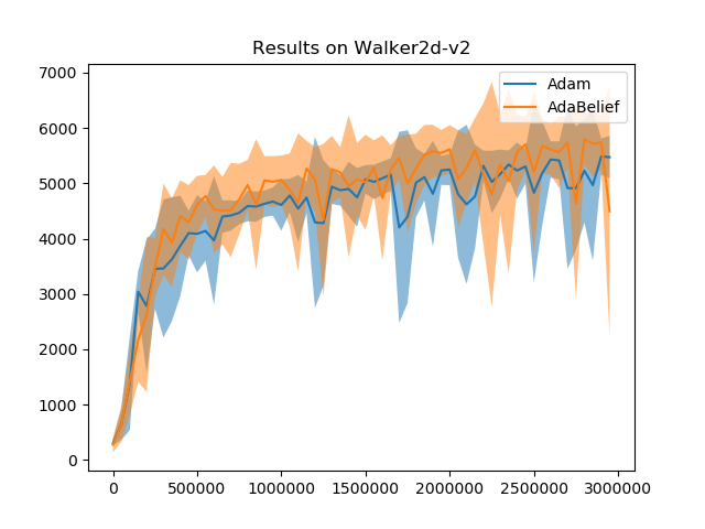
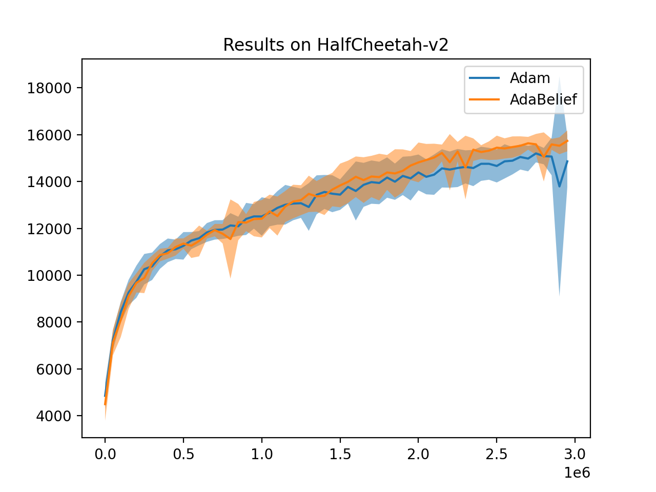
We conducted reinforcement learning with SAC (soft actor critic) [46] in the PFRL package [47]. We plot the reward vs. training step in Fig. 8. AdaBelief achieves higher reward value than Adam.
Refer to caption
((a)) Reward vs. training steps on HalfCheetah-v2.
Refer to caption
((b)) Reward vs. training steps on Walker2d-v2.
Figure 8: Reward vs. training step with SAC model.

4 Related works

This work considers the update step in first-order methods. Other directions include Lookahead [48] which updates “fast” and “slow” weights separately, and is a wrapper that can combine with other optimizers; variance reduction methods [49, 50, 51] which reduce the variance in gradient; and LARS [52] which uses a layer-wise learning rate scaling. AdaBelief can be combined with these methods. Other variants of Adam have also been proposed (e.g. NosAdam [53], Sadam [54] and Adax [55]).

Besides first-order methods, second-order methods (e.g. Newton’s method [56], Quasi-Newton method and Gauss-Newton method [57, 58, 57], L-BFGS [59], Natural-Gradient [60, 61], Conjugate-Gradient [62]) are widely used in conventional optimization. Hessian-free optimization (HFO) [63] uses second-order methods to train neural networks. Second-order methods typically use curvature information and are invariant to scaling [64] but have heavy computational burden, and hence are not widely used in deep learning.

5 Conclusion

We propose the AdaBelief optimizer, which adaptively scales the stepsize by the difference between predicted gradient and observed gradient. To our knowledge, AdaBelief is the first optimizer to achieve three goals simultaneously: fast convergence as in adaptive methods, good generalization as in SGD, and training stability in complex settings such as GANs. Furthermore, Adabelief has the same parameters as Adam, hence is easy to tune. We validate the benefits of AdaBelief with intuitive examples, theoretical convergence analysis in both convex and non-convex cases, and extensive experiments on real-world datasets.

Broader Impact

Optimization is at the core of modern machine learning, and numerous efforts have been put into it. To our knowledge, AdaBelief is the first optimizer to achieve fast speed, good generalization and training stability. Adabelief can be used for the training of all models that can numerically estimate parameter gradients, hence can boost the development and application of deep learning models. This work mainly focuses on the theory part, and the social impact is mainly determined by each application rather than by optimizer.

Acknowledgments and Disclosure of Funding

This research is supported by NIH grant R01NS035193.

References

  • [1] Herbert Robbins and Sutton Monro, “A stochastic approximation method,” The annals of mathematical statistics, pp. 400–407, 1951.
  • [2] Yu Nesterov, “A method of solving a convex programming problem with convergence rate o(1/k2̂),” in Sov. Math. Dokl, 1983, vol. 27.
  • [3] Ilya Sutskever, James Martens, George Dahl, and Geoffrey Hinton, “On the importance of initialization and momentum in deep learning,” in International conference on machine learning, 2013, pp. 1139–1147.
  • [4] Boris T Polyak, “Some methods of speeding up the convergence of iteration methods,” USSR Computational Mathematics and Mathematical Physics, vol. 4, no. 5, pp. 1–17, 1964.
  • [5] John Duchi, Elad Hazan, and Yoram Singer, “Adaptive subgradient methods for online learning and stochastic optimization,” Journal of machine learning research, vol. 12, no. Jul, pp. 2121–2159, 2011.
  • [6] Matthew D Zeiler, “Adadelta: an adaptive learning rate method,” arXiv preprint arXiv:1212.5701, 2012.
  • [7] Alex Graves, “Generating sequences with recurrent neural networks,” arXiv preprint arXiv:1308.0850, 2013.
  • [8] Diederik P Kingma and Jimmy Ba, “Adam: A method for stochastic optimization,” arXiv preprint arXiv:1412.6980, 2014.
  • [9] Ashia C Wilson, Rebecca Roelofs, Mitchell Stern, Nati Srebro, and Benjamin Recht, “The marginal value of adaptive gradient methods in machine learning,” in Advances in Neural Information Processing Systems, 2017, pp. 4148–4158.
  • [10] Kaifeng Lyu and Jian Li, “Gradient descent maximizes the margin of homogeneous neural networks,” arXiv preprint arXiv:1906.05890, 2019.
  • [11] Nitish Shirish Keskar and Richard Socher, “Improving generalization performance by switching from adam to sgd,” arXiv preprint arXiv:1712.07628, 2017.
  • [12] Liangchen Luo, Yuanhao Xiong, Yan Liu, and Xu Sun, “Adaptive gradient methods with dynamic bound of learning rate,” arXiv preprint arXiv:1902.09843, 2019.
  • [13] Sashank J Reddi, Satyen Kale, and Sanjiv Kumar, “On the convergence of adam and beyond,” arXiv preprint arXiv:1904.09237, 2019.
  • [14] Manzil Zaheer, Sashank Reddi, Devendra Sachan, Satyen Kale, and Sanjiv Kumar, “Adaptive methods for nonconvex optimization,” in Advances in neural information processing systems, 2018, pp. 9793–9803.
  • [15] Lukas Balles and Philipp Hennig, “Dissecting adam: The sign, magnitude and variance of stochastic gradients,” arXiv preprint arXiv:1705.07774, 2017.
  • [16] Liyuan Liu, Haoming Jiang, Pengcheng He, Weizhu Chen, Xiaodong Liu, Jianfeng Gao, and Jiawei Han, “On the variance of the adaptive learning rate and beyond,” arXiv preprint arXiv:1908.03265, 2019.
  • [17] Jeremy Bernstein, Arash Vahdat, Yisong Yue, and Ming-Yu Liu, “On the distance between two neural networks and the stability of learning,” arXiv preprint arXiv:2002.03432, 2020.
  • [18] Ilya Loshchilov and Frank Hutter, “Decoupled weight decay regularization,” arXiv preprint arXiv:1711.05101, 2017.
  • [19] Olga Russakovsky, Jia Deng, Hao Su, Jonathan Krause, Sanjeev Satheesh, Sean Ma, Zhiheng Huang, Andrej Karpathy, Aditya Khosla, Michael Bernstein, et al., “Imagenet large scale visual recognition challenge,” International journal of computer vision, vol. 115, no. 3, pp. 211–252, 2015.
  • [20] Ian Goodfellow, Jean Pouget-Abadie, Mehdi Mirza, Bing Xu, David Warde-Farley, Sherjil Ozair, Aaron Courville, and Yoshua Bengio, “Generative adversarial nets,” in Advances in neural information processing systems, 2014, pp. 2672–2680.
  • [21] Martin Arjovsky, Soumith Chintala, and Léon Bottou, “Wasserstein gan,” arXiv preprint arXiv:1701.07875, 2017.
  • [22] Marc Toussaint, “Lecture notes: Some notes on gradient descent,” 2012.
  • [23] Jeremy Bernstein, Yu-Xiang Wang, Kamyar Azizzadenesheli, and Anima Anandkumar, “signsgd: Compressed optimisation for non-convex problems,” arXiv preprint arXiv:1802.04434, 2018.
  • [24] Evelyn ML Beale, “On minimizing a convex function subject to linear inequalities,” Journal of the Royal Statistical Society: Series B (Methodological), vol. 17, no. 2, pp. 173–184, 1955.
  • [25] HoHo Rosenbrock, “An automatic method for finding the greatest or least value of a function,” The Computer Journal, vol. 3, no. 3, pp. 175–184, 1960.
  • [26] Xavier Glorot, Antoine Bordes, and Yoshua Bengio, “Deep sparse rectifier neural networks,” in Proceedings of the fourteenth international conference on artificial intelligence and statistics, 2011, pp. 315–323.
  • [27] Xiangyi Chen, Sijia Liu, Ruoyu Sun, and Mingyi Hong, “On the convergence of a class of adam-type algorithms for non-convex optimization,” arXiv preprint arXiv:1808.02941, 2018.
  • [28] Alex Krizhevsky, Geoffrey Hinton, et al., “Learning multiple layers of features from tiny images,” 2009.
  • [29] Karen Simonyan and Andrew Zisserman, “Very deep convolutional networks for large-scale image recognition,” arXiv preprint arXiv:1409.1556, 2014.
  • [30] Kaiming He, Xiangyu Zhang, Shaoqing Ren, and Jian Sun, “Deep residual learning for image recognition,” in Proceedings of the IEEE conference on computer vision and pattern recognition, 2016, pp. 770–778.
  • [31] Gao Huang, Zhuang Liu, Laurens Van Der Maaten, and Kilian Q Weinberger, “Densely connected convolutional networks,” in Proceedings of the IEEE conference on computer vision and pattern recognition, 2017, pp. 4700–4708.
  • [32] Jia Deng, Wei Dong, Richard Socher, Li-Jia Li, Kai Li, and Li Fei-Fei, “Imagenet: A large-scale hierarchical image database,” in 2009 IEEE conference on computer vision and pattern recognition. Ieee, 2009, pp. 248–255.
  • [33] Xiaolei Ma, Zhimin Tao, Yinhai Wang, Haiyang Yu, and Yunpeng Wang, “Long short-term memory neural network for traffic speed prediction using remote microwave sensor data,” Transportation Research Part C: Emerging Technologies, vol. 54, pp. 187–197, 2015.
  • [34] Mitchell Marcus, Beatrice Santorini, and Mary Ann Marcinkiewicz, “Building a large annotated corpus of english: The penn treebank,” 1993.
  • [35] Jinghui Chen and Quanquan Gu, “Closing the generalization gap of adaptive gradient methods in training deep neural networks,” arXiv preprint arXiv:1806.06763, 2018.
  • [36] Alec Radford, Luke Metz, and Soumith Chintala, “Unsupervised representation learning with deep convolutional generative adversarial networks,” arXiv preprint arXiv:1511.06434, 2015.
  • [37] Tim Salimans, Ian Goodfellow, Wojciech Zaremba, Vicki Cheung, Alec Radford, and Xi Chen, “Improved techniques for training gans,” in Advances in neural information processing systems, 2016, pp. 2234–2242.
  • [38] Ian Goodfellow, “Nips 2016 tutorial: Generative adversarial networks,” arXiv preprint arXiv:1701.00160, 2016.
  • [39] Ishaan Gulrajani, Faruk Ahmed, Martin Arjovsky, Vincent Dumoulin, and Aaron C Courville, “Improved training of wasserstein gans,” in Advances in neural information processing systems, 2017, pp. 5767–5777.
  • [40] Martin Heusel, Hubert Ramsauer, Thomas Unterthiner, Bernhard Nessler, and Sepp Hochreiter, “Gans trained by a two time-scale update rule converge to a local nash equilibrium,” in Advances in neural information processing systems, 2017, pp. 6626–6637.
  • [41] Dongruo Zhou, Yiqi Tang, Ziyan Yang, Yuan Cao, and Quanquan Gu, “On the convergence of adaptive gradient methods for nonconvex optimization,” arXiv preprint arXiv:1808.05671, 2018.
  • [42] Ashish Vaswani, Noam Shazeer, Niki Parmar, Jakob Uszkoreit, Llion Jones, Aidan N Gomez, Łukasz Kaiser, and Illia Polosukhin, “Attention is all you need,” Advances in neural information processing systems, vol. 30, pp. 5998–6008, 2017.
  • [43] Zhewei Yao, Amir Gholami, Sheng Shen, Kurt Keutzer, and Michael W Mahoney, “Adahessian: An adaptive second order optimizer for machine learning,” arXiv preprint arXiv:2006.00719, 2020.
  • [44] Shaoqing Ren, Kaiming He, Ross Girshick, and Jian Sun, “Faster r-cnn: Towards real-time object detection with region proposal networks,” IEEE transactions on pattern analysis and machine intelligence, vol. 39, no. 6, pp. 1137–1149, 2016.
  • [45] Wei Yuan and Kai-Xin Gao, “Eadam optimizer: How epsilon impact adam,” arXiv preprint arXiv:2011.02150, 2020.
  • [46] Tuomas Haarnoja, Aurick Zhou, Pieter Abbeel, and Sergey Levine, “Soft actor-critic: Off-policy maximum entropy deep reinforcement learning with a stochastic actor,” arXiv preprint arXiv:1801.01290, 2018.
  • [47] Yasuhiro Fujita, Toshiki Kataoka, Prabhat Nagarajan, and Takahiro Ishikawa, “Chainerrl: A deep reinforcement learning library,” in Workshop on Deep Reinforcement Learning at the 33rd Conference on Neural Information Processing Systems, December 2019.
  • [48] Michael Zhang, James Lucas, Jimmy Ba, and Geoffrey E Hinton, “Lookahead optimizer: k steps forward, 1 step back,” in Advances in Neural Information Processing Systems, 2019, pp. 9593–9604.
  • [49] Sashank J Reddi, Ahmed Hefny, Suvrit Sra, Barnabás Póczos, and Alex Smola, “Stochastic variance reduction for nonconvex optimization,” in International conference on machine learning, 2016, pp. 314–323.
  • [50] Rie Johnson and Tong Zhang, “Accelerating stochastic gradient descent using predictive variance reduction,” in Advances in neural information processing systems, 2013, pp. 315–323.
  • [51] Jerry Ma and Denis Yarats, “Quasi-hyperbolic momentum and adam for deep learning,” arXiv preprint arXiv:1810.06801, 2018.
  • [52] Yang You, Igor Gitman, and Boris Ginsburg, “Scaling sgd batch size to 32k for imagenet training,” arXiv preprint arXiv:1708.03888, vol. 6, 2017.
  • [53] Haiwen Huang, Chang Wang, and Bin Dong, “Nostalgic adam: Weighting more of the past gradients when designing the adaptive learning rate,” arXiv preprint arXiv:1805.07557, 2018.
  • [54] Guanghui Wang, Shiyin Lu, Weiwei Tu, and Lijun Zhang, “Sadam: A variant of adam for strongly convex functions,” arXiv preprint arXiv:1905.02957, 2019.
  • [55] Wenjie Li, Zhaoyang Zhang, Xinjiang Wang, and Ping Luo, “Adax: Adaptive gradient descent with exponential long term memory,” arXiv preprint arXiv:2004.09740, 2020.
  • [56] Stephen Boyd, Stephen P Boyd, and Lieven Vandenberghe, Convex optimization, Cambridge university press, 2004.
  • [57] Robert WM Wedderburn, “Quasi-likelihood functions, generalized linear models, and the gauss—newton method,” Biometrika, vol. 61, no. 3, pp. 439–447, 1974.
  • [58] Nicol N Schraudolph, “Fast curvature matrix-vector products for second-order gradient descent,” Neural computation, vol. 14, no. 7, pp. 1723–1738, 2002.
  • [59] Jorge Nocedal, “Updating quasi-newton matrices with limited storage,” Mathematics of computation, vol. 35, no. 151, pp. 773–782, 1980.
  • [60] Shun-Ichi Amari, “Natural gradient works efficiently in learning,” Neural computation, vol. 10, no. 2, pp. 251–276, 1998.
  • [61] Razvan Pascanu and Yoshua Bengio, “Revisiting natural gradient for deep networks,” arXiv preprint arXiv:1301.3584, 2013.
  • [62] Magnus R Hestenes, Eduard Stiefel, et al., “Methods of conjugate gradients for solving linear systems,” Journal of research of the National Bureau of Standards, vol. 49, no. 6, pp. 409–436, 1952.
  • [63] James Martens, “Deep learning via hessian-free optimization.,” in ICML, 2010, vol. 27, pp. 735–742.
  • [64] Roberto Battiti, “First-and second-order methods for learning: between steepest descent and newton’s method,” Neural computation, vol. 4, no. 2, pp. 141–166, 1992.
  • [65] H Brendan McMahan and Matthew Streeter, “Adaptive bound optimization for online convex optimization,” arXiv preprint arXiv:1002.4908, 2010.
  • [66] Nicolas L Roux, Pierre-Antoine Manzagol, and Yoshua Bengio, “Topmoumoute online natural gradient algorithm,” in Advances in neural information processing systems, 2008, pp. 849–856.

Appendix

A. Detailed Algorithm of AdaBelief

Notations

By the convention in [8], we use the following notations:

  • f(θ),θdformulae-sequence𝑓𝜃𝜃superscript𝑑f(\theta)\in\mathbb{R},\theta\in\mathbb{R}^{d}: f𝑓f is the loss function to minimize, θ𝜃\theta is the parameter in dsuperscript𝑑\mathbb{R}^{d}

  • gtsubscript𝑔𝑡g_{t}: the gradient and step t𝑡t

  • α,ϵ𝛼italic-ϵ\alpha,\epsilon: α𝛼\alpha is the learning rate, default is 103superscript10310^{-3}; ϵitalic-ϵ\epsilon is a small number, typically set as 108superscript10810^{-8}

  • β1,β2subscript𝛽1subscript𝛽2\beta_{1},\beta_{2}: smoothing parameters, typical values are β1=0.9,β2=0.999formulae-sequencesubscript𝛽10.9subscript𝛽20.999\beta_{1}=0.9,\beta_{2}=0.999

  • mtsubscript𝑚𝑡m_{t}: exponential moving average (EMA) of gtsubscript𝑔𝑡g_{t}

  • vt,stsubscript𝑣𝑡subscript𝑠𝑡v_{t},s_{t}: vtsubscript𝑣𝑡v_{t} is the EMA of gt2superscriptsubscript𝑔𝑡2g_{t}^{2}, stsubscript𝑠𝑡s_{t} is the EMA of (gtmt)2superscriptsubscript𝑔𝑡subscript𝑚𝑡2(g_{t}-m_{t})^{2}

  • ,M(y)=argminxM1/2(xy)subscriptproduct𝑀𝑦subscriptargmin𝑥normsuperscript𝑀12𝑥𝑦\prod_{\mathcal{F},M}(y)=\mathrm{argmin}_{x\in\mathcal{F}}||M^{1/2}(x-y)||

Initialize θ0subscript𝜃0\theta_{0}
               m00subscript𝑚00m_{0}\leftarrow 0 , s00subscript𝑠00s_{0}\leftarrow 0, t0𝑡0t\leftarrow 0
While θtsubscript𝜃𝑡\theta_{t} not converged
               tt+1𝑡𝑡1t\leftarrow t+1
               gtθft(θt1)subscript𝑔𝑡subscript𝜃subscript𝑓𝑡subscript𝜃𝑡1g_{t}\leftarrow\nabla_{\theta}f_{t}(\theta_{t-1})
               mtβ1mt1+(1β1)gtsubscript𝑚𝑡subscript𝛽1subscript𝑚𝑡11subscript𝛽1subscript𝑔𝑡m_{t}\leftarrow\beta_{1}m_{t-1}+(1-\beta_{1})g_{t}
               stβ2st1+(1β2)(gtmt)2+ϵsubscript𝑠𝑡subscript𝛽2subscript𝑠𝑡11subscript𝛽2superscriptsubscript𝑔𝑡subscript𝑚𝑡2italic-ϵs_{t}\leftarrow\beta_{2}s_{t-1}+(1-\beta_{2}){\color[rgb]{0,0,0}\definecolor[named]{pgfstrokecolor}{rgb}{0,0,0}\pgfsys@color@gray@stroke{0}\pgfsys@color@gray@fill{0}(g_{t}-m_{t})^{2}}+\epsilon
               If AMSGrad𝐴𝑀𝑆𝐺𝑟𝑎𝑑AMSGrad
                      stmax(st,st1)subscript𝑠𝑡maxsubscript𝑠𝑡subscript𝑠𝑡1{\color[rgb]{0,0,0}\definecolor[named]{pgfstrokecolor}{rgb}{0,0,0}\pgfsys@color@gray@stroke{0}\pgfsys@color@gray@fill{0}{s_{t}\leftarrow\operatorname{max}(s_{t},s_{t-1})}}
               Bias Correction
                      mt^mt/(1β1t)^subscript𝑚𝑡subscript𝑚𝑡1superscriptsubscript𝛽1𝑡\widehat{m_{t}}\leftarrow m_{t}/(1-\beta_{1}^{t}),         st^(st)/(1β2t)^subscript𝑠𝑡subscript𝑠𝑡1superscriptsubscript𝛽2𝑡\widehat{s_{t}}\leftarrow(s_{t})/(1-\beta_{2}^{t})
               Update
                      θt,st(θt1mt^αst^+ϵ)subscript𝜃𝑡subscriptproductsubscript𝑠𝑡subscript𝜃𝑡1^subscript𝑚𝑡𝛼^subscript𝑠𝑡italic-ϵ\theta_{t}\leftarrow\prod_{\mathcal{F},\sqrt{s_{t}}}\Big{(}\theta_{t-1}-\widehat{m_{t}}\frac{\alpha}{\sqrt{\widehat{s_{t}}}+\epsilon}\Big{)}
Algorithm 3 AdaBelief

B. Convergence analysis in convex online learning case (Theorem 2.1 in main paper)

For the ease of notation, we absorb ϵitalic-ϵ\epsilon into stsubscript𝑠𝑡s_{t}. Equivalently, stc>0,t[T]formulae-sequencesubscript𝑠𝑡𝑐0for-all𝑡delimited-[]𝑇s_{t}\geq c>0,\forall t\in[T]. For simplicity, we omit the debiasing step in theoretical analysis as in [13]. Our analysis can be applied to the de-biased version as well.

Lemma .1.

[65] For any QS+d𝑄subscriptsuperscript𝑆𝑑Q\in S^{d}_{+} and convex feasible set dsuperscript𝑑\mathcal{F}\subset\mathbb{R}^{d}, suppose u1=minxQ1/2(xz1)subscript𝑢1subscriptmin𝑥normsuperscript𝑄12𝑥subscript𝑧1u_{1}=\operatorname*{min}_{x\in\mathcal{F}}\Big{|}\Big{|}Q^{1/2}(x-z_{1})\Big{|}\Big{|} and u2=minxQ1/2(xz2)subscript𝑢2subscriptmin𝑥normsuperscript𝑄12𝑥subscript𝑧2u_{2}=\operatorname*{min}_{x\in\mathcal{F}}\Big{|}\Big{|}Q^{1/2}(x-z_{2})\Big{|}\Big{|}, then we have Q1/2(u1u2)Q1/2(z1z2)normsuperscript𝑄12subscript𝑢1subscript𝑢2normsuperscript𝑄12subscript𝑧1subscript𝑧2\Big{|}\Big{|}Q^{1/2}(u_{1}-u_{2})\Big{|}\Big{|}\leq\Big{|}\Big{|}Q^{1/2}(z_{1}-z_{2})\Big{|}\Big{|}.

Theorem .2.

Let {θt}subscript𝜃𝑡\{\theta_{t}\} and {st}subscript𝑠𝑡\{s_{t}\} be the sequence obtained by the proposed algorithm, let 0β2<1,αt=αtformulae-sequence0subscript𝛽21subscript𝛼𝑡𝛼𝑡0\leq\beta_{2}<1,\alpha_{t}=\frac{\alpha}{\sqrt{t}}, β11=β1subscript𝛽11subscript𝛽1\beta_{11}=\beta_{1}, 0β1tβ1<1,st1st,t[T]formulae-sequence0subscript𝛽1𝑡subscript𝛽11formulae-sequencesubscript𝑠𝑡1subscript𝑠𝑡for-all𝑡delimited-[]𝑇0\leq\beta_{1t}\leq\beta_{1}<1,s_{t-1}\leq s_{t},\forall t\in[T]. Let θ𝜃\theta\in\mathcal{F}, where dsuperscript𝑑\mathcal{F}\subset\mathbb{R}^{d} is a convex feasible set with bounded diameter Dsubscript𝐷D_{\infty}. Assume f(θ)𝑓𝜃f(\theta) is a convex function and gtG/2subscriptnormsubscript𝑔𝑡subscript𝐺2||g_{t}||_{\infty}\leq G_{\infty}/2 (hence gtmtGsubscriptnormsubscript𝑔𝑡subscript𝑚𝑡subscript𝐺||g_{t}-m_{t}||_{\infty}\leq G_{\infty}) and st,ic>0,t[T],θformulae-sequencesubscript𝑠𝑡𝑖𝑐0formulae-sequencefor-all𝑡delimited-[]𝑇𝜃s_{t,i}\geq c>0,\forall t\in[T],\theta\in\mathcal{F}. Denote the optimal point as θsuperscript𝜃\theta^{*}. For θtsubscript𝜃𝑡\theta_{t} generated with Algorithm 3, we have the following bound on the regret:

t=1Tft(θt)ft(θ)superscriptsubscript𝑡1𝑇subscript𝑓𝑡subscript𝜃𝑡subscript𝑓𝑡superscript𝜃\displaystyle\sum_{t=1}^{T}f_{t}(\theta_{t})-f_{t}(\theta^{*}) D2T2α(1β1)i=1dsT,i1/2+(1+β1)α1+logT2c(1β1)3i=1dg1:T,i22absentsuperscriptsubscript𝐷2𝑇2𝛼1subscript𝛽1superscriptsubscript𝑖1𝑑superscriptsubscript𝑠𝑇𝑖121subscript𝛽1𝛼1𝑇2𝑐superscript1subscript𝛽13superscriptsubscript𝑖1𝑑subscriptnormsuperscriptsubscript𝑔:1𝑇𝑖22\displaystyle\leq\frac{D_{\infty}^{2}\sqrt{T}}{2\alpha(1-\beta_{1})}\sum_{i=1}^{d}s_{T,i}^{1/2}+\frac{(1+\beta_{1})\alpha\sqrt{1+\log T}}{2\sqrt{c}(1-\beta_{1})^{3}}\sum_{i=1}^{d}\Big{|}\Big{|}g_{1:T,i}^{2}\Big{|}\Big{|}_{2}
+D22(1β1)t=1Ti=1dβ1tst,i1/2αtsuperscriptsubscript𝐷221subscript𝛽1superscriptsubscript𝑡1𝑇superscriptsubscript𝑖1𝑑subscript𝛽1𝑡superscriptsubscript𝑠𝑡𝑖12subscript𝛼𝑡\displaystyle+\frac{D_{\infty}^{2}}{2(1-\beta_{1})}\sum_{t=1}^{T}\sum_{i=1}^{d}\frac{\beta_{1t}s_{t,i}^{1/2}}{\alpha_{t}}

Proof:

θt+1=,st(θtαtst1/2mt)=minθst1/4[θ(θtαtst1/2mt)]subscript𝜃𝑡1subscriptproductsubscript𝑠𝑡subscript𝜃𝑡subscript𝛼𝑡superscriptsubscript𝑠𝑡12subscript𝑚𝑡subscriptmin𝜃normsuperscriptsubscript𝑠𝑡14delimited-[]𝜃subscript𝜃𝑡subscript𝛼𝑡superscriptsubscript𝑠𝑡12subscript𝑚𝑡\theta_{t+1}=\prod_{\mathcal{F},\sqrt{s_{t}}}(\theta_{t}-\alpha_{t}s_{t}^{-1/2}m_{t})=\operatorname*{min}_{\theta\in\mathcal{F}}\Big{|}\Big{|}s_{t}^{1/4}[\theta-(\theta_{t}-\alpha_{t}s_{t}^{-1/2}m_{t})]\Big{|}\Big{|}

Note that ,st(θ)=θsubscriptproductsubscript𝑠𝑡superscript𝜃superscript𝜃\prod_{\mathcal{F},\sqrt{s_{t}}}(\theta^{*})=\theta^{*} since θsuperscript𝜃\theta^{*}\in\mathcal{F}. Use θisubscriptsuperscript𝜃𝑖\theta^{*}_{i} and θt,isubscript𝜃𝑡𝑖\theta_{t,i} to denote the i𝑖ith dimension of θsuperscript𝜃\theta^{*} and θtsubscript𝜃𝑡\theta_{t} respectively. From lemma (.1), using u1=θt+1subscript𝑢1subscript𝜃𝑡1u_{1}=\theta_{t+1} and u2=θsubscript𝑢2superscript𝜃u_{2}=\theta^{*}, we have:

st1/4(θt+1θ)2superscriptnormsuperscriptsubscript𝑠𝑡14subscript𝜃𝑡1superscript𝜃2\displaystyle\Big{|}\Big{|}s_{t}^{1/4}(\theta_{t+1}-\theta^{*})\Big{|}\Big{|}^{2} st1/4(θtαtst1/2mtθ)2absentsuperscriptnormsuperscriptsubscript𝑠𝑡14subscript𝜃𝑡subscript𝛼𝑡superscriptsubscript𝑠𝑡12subscript𝑚𝑡superscript𝜃2\displaystyle\leq\Big{|}\Big{|}s_{t}^{1/4}(\theta_{t}-\alpha_{t}s_{t}^{-1/2}m_{t}-\theta^{*})\Big{|}\Big{|}^{2}
=st1/4(θtθ)2+αt2st1/4mt22αtmt,θtθabsentsuperscriptnormsuperscriptsubscript𝑠𝑡14subscript𝜃𝑡superscript𝜃2superscriptsubscript𝛼𝑡2superscriptnormsuperscriptsubscript𝑠𝑡14subscript𝑚𝑡22subscript𝛼𝑡subscript𝑚𝑡subscript𝜃𝑡superscript𝜃\displaystyle=\Big{|}\Big{|}s_{t}^{1/4}(\theta_{t}-\theta^{*})\Big{|}\Big{|}^{2}+\alpha_{t}^{2}\Big{|}\Big{|}s_{t}^{-1/4}m_{t}\Big{|}\Big{|}^{2}-2\alpha_{t}\langle m_{t},\theta_{t}-\theta^{*}\rangle
=st1/4(θtθ)2+αt2st1/4mt2absentsuperscriptnormsuperscriptsubscript𝑠𝑡14subscript𝜃𝑡superscript𝜃2superscriptsubscript𝛼𝑡2superscriptnormsuperscriptsubscript𝑠𝑡14subscript𝑚𝑡2\displaystyle=\Big{|}\Big{|}s_{t}^{1/4}(\theta_{t}-\theta^{*})\Big{|}\Big{|}^{2}+\alpha_{t}^{2}\Big{|}\Big{|}s_{t}^{-1/4}m_{t}\Big{|}\Big{|}^{2}
2αtβ1tmt1+(1β1t)gt,θtθ2subscript𝛼𝑡subscript𝛽1𝑡subscript𝑚𝑡11subscript𝛽1𝑡subscript𝑔𝑡subscript𝜃𝑡superscript𝜃\displaystyle-2\alpha_{t}\langle\beta_{1t}m_{t-1}+(1-\beta_{1t})g_{t},\theta_{t}-\theta^{*}\rangle (1)

Note that β1[0,1)subscript𝛽101\beta_{1}\in[0,1) and β2[0,1)subscript𝛽201\beta_{2}\in[0,1), rearranging inequality (B. Convergence analysis in convex online learning case (Theorem 2.1 in main paper)), we have:

gt,θtθsubscript𝑔𝑡subscript𝜃𝑡superscript𝜃\displaystyle\langle g_{t},\theta_{t}-\theta^{*}\rangle 12αt(1β1t)[st1/4(θtθ)2st1/4(θt+1θ)2]absent12subscript𝛼𝑡1subscript𝛽1𝑡delimited-[]superscriptnormsuperscriptsubscript𝑠𝑡14subscript𝜃𝑡superscript𝜃2superscriptnormsuperscriptsubscript𝑠𝑡14subscript𝜃𝑡1superscript𝜃2\displaystyle\leq\frac{1}{2\alpha_{t}(1-\beta_{1t})}\Big{[}\Big{|}\Big{|}s_{t}^{1/4}(\theta_{t}-\theta^{*})\Big{|}\Big{|}^{2}-\Big{|}\Big{|}s_{t}^{1/4}(\theta_{t+1}-\theta^{*})\Big{|}\Big{|}^{2}\Big{]}
+αt2(1β1t)st1/4mt2β1t1β1tmt1,θtθsubscript𝛼𝑡21subscript𝛽1𝑡superscriptnormsuperscriptsubscript𝑠𝑡14subscript𝑚𝑡2subscript𝛽1𝑡1subscript𝛽1𝑡subscript𝑚𝑡1subscript𝜃𝑡superscript𝜃\displaystyle+\frac{\alpha_{t}}{2(1-\beta_{1t})}\Big{|}\Big{|}s_{t}^{-1/4}m_{t}\Big{|}\Big{|}^{2}-\frac{\beta_{1t}}{1-\beta_{1t}}\langle m_{t-1},\theta_{t}-\theta^{*}\rangle
12αt(1β1t)[st1/4(θtθ)2st1/4(θt+1θ)2]absent12subscript𝛼𝑡1subscript𝛽1𝑡delimited-[]superscriptnormsuperscriptsubscript𝑠𝑡14subscript𝜃𝑡superscript𝜃2superscriptnormsuperscriptsubscript𝑠𝑡14subscript𝜃𝑡1superscript𝜃2\displaystyle\leq\frac{1}{2\alpha_{t}(1-\beta_{1t})}\Big{[}\Big{|}\Big{|}s_{t}^{1/4}(\theta_{t}-\theta^{*})\Big{|}\Big{|}^{2}-\Big{|}\Big{|}s_{t}^{1/4}(\theta_{t+1}-\theta^{*})\Big{|}\Big{|}^{2}\Big{]}
+αt2(1β1t)st1/4mt2subscript𝛼𝑡21subscript𝛽1𝑡superscriptnormsuperscriptsubscript𝑠𝑡14subscript𝑚𝑡2\displaystyle+\frac{\alpha_{t}}{2(1-\beta_{1t})}\Big{|}\Big{|}s_{t}^{-1/4}m_{t}\Big{|}\Big{|}^{2}
+β1t2(1β1t)αtst1/4mt12+β1t2αt(1β1t)st1/4(θtθ)2subscript𝛽1𝑡21subscript𝛽1𝑡subscript𝛼𝑡superscriptnormsuperscriptsubscript𝑠𝑡14subscript𝑚𝑡12subscript𝛽1𝑡2subscript𝛼𝑡1subscript𝛽1𝑡superscriptnormsuperscriptsubscript𝑠𝑡14subscript𝜃𝑡superscript𝜃2\displaystyle+\frac{\beta_{1t}}{2(1-\beta_{1t})}\alpha_{t}\Big{|}\Big{|}s_{t}^{-1/4}m_{t-1}\Big{|}\Big{|}^{2}+\frac{\beta_{1t}}{2\alpha_{t}(1-\beta_{1t})}\Big{|}\Big{|}s_{t}^{1/4}(\theta_{t}-\theta^{*})\Big{|}\Big{|}^{2}
(Cauchy-Schwartz and Young’s inequality: aba2ϵ2+b22ϵ,ϵ>0)formulae-sequenceCauchy-Schwartz and Young’s inequality: 𝑎𝑏superscript𝑎2italic-ϵ2superscript𝑏22italic-ϵfor-allitalic-ϵ0\displaystyle\Big{(}\textit{Cauchy-Schwartz and Young's inequality: }ab\leq\frac{a^{2}\epsilon}{2}+\frac{b^{2}}{2\epsilon},\forall\epsilon>0\Big{)} (2)

By convexity of f𝑓f, we have:

t=1Tft(θt)ft(θ)superscriptsubscript𝑡1𝑇subscript𝑓𝑡subscript𝜃𝑡subscript𝑓𝑡superscript𝜃\displaystyle\sum_{t=1}^{T}f_{t}(\theta_{t})-f_{t}(\theta^{*}) t=1Tgt,θtθabsentsuperscriptsubscript𝑡1𝑇subscript𝑔𝑡subscript𝜃𝑡superscript𝜃\displaystyle\leq\sum_{t=1}^{T}\langle g_{t},\theta_{t}-\theta^{*}\rangle
t=1T{12αt(1β1t)[||st1/4(θtθ)||2||st1/4(θt+1θ)||2]\displaystyle\leq\sum_{t=1}^{T}\Big{\{}\frac{1}{2\alpha_{t}(1-\beta_{1t})}\Big{[}\Big{|}\Big{|}s_{t}^{1/4}(\theta_{t}-\theta^{*})\Big{|}\Big{|}^{2}-\Big{|}\Big{|}s_{t}^{1/4}(\theta_{t+1}-\theta^{*})\Big{|}\Big{|}^{2}\Big{]}
+12(1β1t)αtst1/4mt2+β1t2(1β1t)αtst1/4mt12121subscript𝛽1𝑡subscript𝛼𝑡superscriptnormsuperscriptsubscript𝑠𝑡14subscript𝑚𝑡2subscript𝛽1𝑡21subscript𝛽1𝑡subscript𝛼𝑡superscriptnormsuperscriptsubscript𝑠𝑡14subscript𝑚𝑡12\displaystyle+\frac{1}{2(1-\beta_{1t})}\alpha_{t}\Big{|}\Big{|}s_{t}^{-1/4}m_{t}\Big{|}\Big{|}^{2}+\frac{\beta_{1t}}{2(1-\beta_{1t})}\alpha_{t}\Big{|}\Big{|}s_{t}^{-1/4}m_{t-1}\Big{|}\Big{|}^{2}
+β1t2αt(1β1t)||st1/4(θtθ)||2}\displaystyle+\frac{\beta_{1t}}{2\alpha_{t}(1-\beta_{1t})}\Big{|}\Big{|}s_{t}^{1/4}(\theta_{t}-\theta^{*})\Big{|}\Big{|}^{2}\Big{\}}
(Byformula(B. Convergence analysis in convex online learning case (Theorem 2.1 in main paper)))𝐵𝑦𝑓𝑜𝑟𝑚𝑢𝑙𝑎italic-(B. Convergence analysis in convex online learning case (Theorem 2.1 in main paper)italic-)\displaystyle\Big{(}By\ formula~{}\eqref{supeq:2}\Big{)}
12(1β1)s11/4(θ1θ)2α1absent121subscript𝛽1superscriptnormsuperscriptsubscript𝑠114subscript𝜃1superscript𝜃2subscript𝛼1\displaystyle\leq\frac{1}{2(1-\beta_{1})}\frac{\Big{|}\Big{|}s_{1}^{1/4}(\theta_{1}-\theta^{*})\Big{|}\Big{|}^{2}}{\alpha_{1}}
+12(1β1)t=2T[st1/4(θtθ)2αtst11/4(θtθ)2αt1]121subscript𝛽1superscriptsubscript𝑡2𝑇delimited-[]superscriptnormsuperscriptsubscript𝑠𝑡14subscript𝜃𝑡superscript𝜃2subscript𝛼𝑡superscriptnormsuperscriptsubscript𝑠𝑡114subscript𝜃𝑡superscript𝜃2subscript𝛼𝑡1\displaystyle+\frac{1}{2(1-\beta_{1})}\sum_{t=2}^{T}\Big{[}\frac{\Big{|}\Big{|}s_{t}^{1/4}(\theta_{t}-\theta^{*})\Big{|}\Big{|}^{2}}{\alpha_{t}}-\frac{\Big{|}\Big{|}s_{t-1}^{1/4}(\theta_{t}-\theta^{*})\Big{|}\Big{|}^{2}}{\alpha_{t-1}}\Big{]}
+t=1T[12(1β1)αtst1/4mt2]+t=2T[β12(1β1)αt1st11/4mt12]superscriptsubscript𝑡1𝑇delimited-[]121subscript𝛽1subscript𝛼𝑡superscriptnormsuperscriptsubscript𝑠𝑡14subscript𝑚𝑡2superscriptsubscript𝑡2𝑇delimited-[]subscript𝛽121subscript𝛽1subscript𝛼𝑡1superscriptnormsuperscriptsubscript𝑠𝑡114subscript𝑚𝑡12\displaystyle+\sum_{t=1}^{T}\Big{[}\frac{1}{2(1-\beta_{1})}\alpha_{t}\Big{|}\Big{|}s_{t}^{-1/4}m_{t}\Big{|}\Big{|}^{2}\Big{]}+\sum_{t=2}^{T}\Big{[}\frac{\beta_{1}}{2(1-\beta_{1})}\alpha_{t-1}\Big{|}\Big{|}s_{t-1}^{-1/4}m_{t-1}\Big{|}\Big{|}^{2}\Big{]}
+t=1Tβ1t2αt(1β1t)st1/4(θtθ)2superscriptsubscript𝑡1𝑇subscript𝛽1𝑡2subscript𝛼𝑡1subscript𝛽1𝑡superscriptnormsuperscriptsubscript𝑠𝑡14subscript𝜃𝑡superscript𝜃2\displaystyle+\sum_{t=1}^{T}\frac{\beta_{1t}}{2\alpha_{t}(1-\beta_{1t})}\Big{|}\Big{|}s_{t}^{1/4}(\theta_{t}-\theta^{*})\Big{|}\Big{|}^{2}
(0st1st,0αtαt1,0β1tβ1<1)formulae-sequence0subscript𝑠𝑡1subscript𝑠𝑡0subscript𝛼𝑡subscript𝛼𝑡10subscript𝛽1𝑡subscript𝛽11\displaystyle\Big{(}0\leq s_{t-1}\leq s_{t},0\leq\alpha_{t}\leq\alpha_{t-1},0\leq\beta_{1t}\leq\beta_{1}<1\Big{)}
12(1β1)s11/4(θ1θ)2α1+12(1β1)t=2Tθtθ2[st1/2αtst11/2αt1]absent121subscript𝛽1superscriptnormsuperscriptsubscript𝑠114subscript𝜃1superscript𝜃2subscript𝛼1121subscript𝛽1superscriptsubscript𝑡2𝑇superscriptnormsubscript𝜃𝑡superscript𝜃2delimited-[]superscriptsubscript𝑠𝑡12subscript𝛼𝑡superscriptsubscript𝑠𝑡112subscript𝛼𝑡1\displaystyle\leq\frac{1}{2(1-\beta_{1})}\frac{\Big{|}\Big{|}s_{1}^{1/4}(\theta_{1}-\theta^{*})\Big{|}\Big{|}^{2}}{\alpha_{1}}+\frac{1}{2(1-\beta_{1})}\sum_{t=2}^{T}\Big{|}\Big{|}\theta_{t}-\theta^{*}\Big{|}\Big{|}^{2}\Big{[}\frac{s_{t}^{1/2}}{\alpha_{t}}-\frac{s_{t-1}^{1/2}}{\alpha_{t-1}}\Big{]}
+1+β12(1β1)t=1Tαtst1/4mt21subscript𝛽121subscript𝛽1superscriptsubscript𝑡1𝑇subscript𝛼𝑡superscriptnormsuperscriptsubscript𝑠𝑡14subscript𝑚𝑡2\displaystyle+\frac{1+\beta_{1}}{2(1-\beta_{1})}\sum_{t=1}^{T}\alpha_{t}\Big{|}\Big{|}s_{t}^{-1/4}m_{t}\Big{|}\Big{|}^{2}
+t=1Tβ1t2αt(1β1t)st1/4(θtθ)2superscriptsubscript𝑡1𝑇subscript𝛽1𝑡2subscript𝛼𝑡1subscript𝛽1𝑡superscriptnormsuperscriptsubscript𝑠𝑡14subscript𝜃𝑡superscript𝜃2\displaystyle+\sum_{t=1}^{T}\frac{\beta_{1t}}{2\alpha_{t}(1-\beta_{1t})}\Big{|}\Big{|}s_{t}^{1/4}(\theta_{t}-\theta^{*})\Big{|}\Big{|}^{2}
12(1β1)s11/4(θ1θ)2α1+12(1β1)t=2Tθtθ2[st1/2αtst11/2αt1]absent121subscript𝛽1superscriptnormsuperscriptsubscript𝑠114subscript𝜃1superscript𝜃2subscript𝛼1121subscript𝛽1superscriptsubscript𝑡2𝑇superscriptnormsubscript𝜃𝑡superscript𝜃2delimited-[]superscriptsubscript𝑠𝑡12subscript𝛼𝑡superscriptsubscript𝑠𝑡112subscript𝛼𝑡1\displaystyle\leq\frac{1}{2(1-\beta_{1})}\frac{\Big{|}\Big{|}s_{1}^{1/4}(\theta_{1}-\theta^{*})\Big{|}\Big{|}^{2}}{\alpha_{1}}+\frac{1}{2(1-\beta_{1})}\sum_{t=2}^{T}\Big{|}\Big{|}\theta_{t}-\theta^{*}\Big{|}\Big{|}^{2}\Big{[}\frac{s_{t}^{1/2}}{\alpha_{t}}-\frac{s_{t-1}^{1/2}}{\alpha_{t-1}}\Big{]}
+1+β12(1β1)t=1Tαtst1/4mt21subscript𝛽121subscript𝛽1superscriptsubscript𝑡1𝑇subscript𝛼𝑡superscriptnormsuperscriptsubscript𝑠𝑡14subscript𝑚𝑡2\displaystyle+\frac{1+\beta_{1}}{2(1-\beta_{1})}\sum_{t=1}^{T}\alpha_{t}\Big{|}\Big{|}s_{t}^{-1/4}m_{t}\Big{|}\Big{|}^{2}
+12(1β1)t=1Tβ1tαtst1/4(θtθ)2121subscript𝛽1superscriptsubscript𝑡1𝑇subscript𝛽1𝑡subscript𝛼𝑡superscriptnormsuperscriptsubscript𝑠𝑡14subscript𝜃𝑡superscript𝜃2\displaystyle+\frac{1}{2(1-\beta_{1})}\sum_{t=1}^{T}\frac{\beta_{1t}}{\alpha_{t}}\Big{|}\Big{|}s_{t}^{1/4}(\theta_{t}-\theta^{*})\Big{|}\Big{|}^{2}
(since 0β1tβ1<1)since 0subscript𝛽1𝑡subscript𝛽11\displaystyle\Big{(}\textit{since\ }0\leq\beta_{1t}\leq\beta_{1}<1\Big{)} (3)

Now bound t=1Tαtst1/4mt2superscriptsubscript𝑡1𝑇subscript𝛼𝑡superscriptnormsuperscriptsubscript𝑠𝑡14subscript𝑚𝑡2\sum_{t=1}^{T}\alpha_{t}||s_{t}^{-1/4}m_{t}||^{2} in Formula  (B. Convergence analysis in convex online learning case (Theorem 2.1 in main paper)), assuming 0<cst,t[T]formulae-sequence0𝑐subscript𝑠𝑡for-all𝑡delimited-[]𝑇0<c\leq s_{t},\forall t\in[T].

t=1Tαtst1/4mt2superscriptsubscript𝑡1𝑇subscript𝛼𝑡superscriptnormsuperscriptsubscript𝑠𝑡14subscript𝑚𝑡2\displaystyle\sum_{t=1}^{T}\alpha_{t}\Big{|}\Big{|}s_{t}^{-1/4}m_{t}\Big{|}\Big{|}^{2} =t=1T1αtst1/4mt2+αTsT1/4mT2absentsuperscriptsubscript𝑡1𝑇1subscript𝛼𝑡superscriptnormsuperscriptsubscript𝑠𝑡14subscript𝑚𝑡2subscript𝛼𝑇superscriptnormsuperscriptsubscript𝑠𝑇14subscript𝑚𝑇2\displaystyle=\sum_{t=1}^{T-1}\alpha_{t}\Big{|}\Big{|}s_{t}^{-1/4}m_{t}\Big{|}\Big{|}^{2}+\alpha_{T}\Big{|}\Big{|}s_{T}^{-1/4}m_{T}\Big{|}\Big{|}^{2}
t=1T1αtst1/4mt2+αTcmT2absentsuperscriptsubscript𝑡1𝑇1subscript𝛼𝑡superscriptnormsuperscriptsubscript𝑠𝑡14subscript𝑚𝑡2subscript𝛼𝑇𝑐superscriptnormsubscript𝑚𝑇2\displaystyle\leq\sum_{t=1}^{T-1}\alpha_{t}\Big{|}\Big{|}s_{t}^{-1/4}m_{t}\Big{|}\Big{|}^{2}+{\color[rgb]{0,0,0}\definecolor[named]{pgfstrokecolor}{rgb}{0,0,0}\pgfsys@color@gray@stroke{0}\pgfsys@color@gray@fill{0}\frac{\alpha_{T}}{\sqrt{c}}\Big{|}\Big{|}m_{T}\Big{|}\Big{|}^{2}}
=t=1T1αtst1/4mt2+αcTi=1d(j=1T(1β1,j)gj,ik=1Tjβ1,Tk+1)2absentsuperscriptsubscript𝑡1𝑇1subscript𝛼𝑡superscriptnormsuperscriptsubscript𝑠𝑡14subscript𝑚𝑡2𝛼𝑐𝑇superscriptsubscript𝑖1𝑑superscriptsuperscriptsubscript𝑗1𝑇1subscript𝛽1𝑗subscript𝑔𝑗𝑖superscriptsubscriptproduct𝑘1𝑇𝑗subscript𝛽1𝑇𝑘12\displaystyle=\sum_{t=1}^{T-1}\alpha_{t}\Big{|}\Big{|}s_{t}^{-1/4}m_{t}\Big{|}\Big{|}^{2}+\frac{\alpha}{\sqrt{cT}}\sum_{i=1}^{d}\Big{(}\sum_{j=1}^{T}(1-\beta_{1,j})g_{j,i}\prod_{k=1}^{T-j}\beta_{1,T-k+1}\Big{)}^{2}
(since mT=j=1T(1β1,j)gj,ik=1Tjβ1,Tk+1)since subscript𝑚𝑇superscriptsubscript𝑗1𝑇1subscript𝛽1𝑗subscript𝑔𝑗𝑖superscriptsubscriptproduct𝑘1𝑇𝑗subscript𝛽1𝑇𝑘1\displaystyle\Big{(}\textit{since\ }m_{T}=\sum_{j=1}^{T}(1-\beta_{1,j})g_{j,i}\prod_{k=1}^{T-j}\beta_{1,T-k+1}\Big{)}
t=1T1αtst1/4mt2+αcTi=1d(j=1Tgj,ik=1Tjβ1)2absentsuperscriptsubscript𝑡1𝑇1subscript𝛼𝑡superscriptnormsuperscriptsubscript𝑠𝑡14subscript𝑚𝑡2𝛼𝑐𝑇superscriptsubscript𝑖1𝑑superscriptsuperscriptsubscript𝑗1𝑇subscript𝑔𝑗𝑖superscriptsubscriptproduct𝑘1𝑇𝑗subscript𝛽12\displaystyle\leq\sum_{t=1}^{T-1}\alpha_{t}\Big{|}\Big{|}s_{t}^{-1/4}m_{t}\Big{|}\Big{|}^{2}+{\color[rgb]{0,0,0}\definecolor[named]{pgfstrokecolor}{rgb}{0,0,0}\pgfsys@color@gray@stroke{0}\pgfsys@color@gray@fill{0}\frac{\alpha}{\sqrt{cT}}\sum_{i=1}^{d}\Big{(}\sum_{j=1}^{T}g_{j,i}\prod_{k=1}^{T-j}\beta_{1}\Big{)}^{2}}
(since 0<β1,jβ1<1)since 0subscript𝛽1𝑗subscript𝛽11\displaystyle(\textit{since \ }0<\beta_{1,j}\leq\beta_{1}<1)
=t=1T1αtst1/4mt2+αcTi=1d(j=1Tβ1Tjgj,i)2absentsuperscriptsubscript𝑡1𝑇1subscript𝛼𝑡superscriptnormsuperscriptsubscript𝑠𝑡14subscript𝑚𝑡2𝛼𝑐𝑇superscriptsubscript𝑖1𝑑superscriptsuperscriptsubscript𝑗1𝑇superscriptsubscript𝛽1𝑇𝑗subscript𝑔𝑗𝑖2\displaystyle=\sum_{t=1}^{T-1}\alpha_{t}\Big{|}\Big{|}s_{t}^{-1/4}m_{t}\Big{|}\Big{|}^{2}+{\color[rgb]{0,0,0}\definecolor[named]{pgfstrokecolor}{rgb}{0,0,0}\pgfsys@color@gray@stroke{0}\pgfsys@color@gray@fill{0}\frac{\alpha}{\sqrt{cT}}\sum_{i=1}^{d}\Big{(}\sum_{j=1}^{T}\beta_{1}^{T-j}g_{j,i}\Big{)}^{2}}
t=1T1αtst1/4mt2+αcTi=1d(j=1Tβ1Tj)(j=1Tβ1Tjgj,i2)absentsuperscriptsubscript𝑡1𝑇1subscript𝛼𝑡superscriptnormsuperscriptsubscript𝑠𝑡14subscript𝑚𝑡2𝛼𝑐𝑇superscriptsubscript𝑖1𝑑superscriptsubscript𝑗1𝑇superscriptsubscript𝛽1𝑇𝑗superscriptsubscript𝑗1𝑇superscriptsubscript𝛽1𝑇𝑗superscriptsubscript𝑔𝑗𝑖2\displaystyle\leq\sum_{t=1}^{T-1}\alpha_{t}\Big{|}\Big{|}s_{t}^{-1/4}m_{t}\Big{|}\Big{|}^{2}+{\color[rgb]{0,0,0}\definecolor[named]{pgfstrokecolor}{rgb}{0,0,0}\pgfsys@color@gray@stroke{0}\pgfsys@color@gray@fill{0}\frac{\alpha}{\sqrt{cT}}\sum_{i=1}^{d}\Big{(}\sum_{j=1}^{T}\beta_{1}^{T-j}\Big{)}\Big{(}\sum_{j=1}^{T}\beta_{1}^{T-j}g_{j,i}^{2}\Big{)}}
(CauchySchwartz,u,v2u2v2,uj=β1Tj,vj=β1Tjgj,i)formulae-sequence𝐶𝑎𝑢𝑐𝑦𝑆𝑐𝑤𝑎𝑟𝑡𝑧superscript𝑢𝑣2superscriptnorm𝑢2superscriptnorm𝑣2formulae-sequencesubscript𝑢𝑗superscriptsubscript𝛽1𝑇𝑗subscript𝑣𝑗superscriptsubscript𝛽1𝑇𝑗subscript𝑔𝑗𝑖\displaystyle\Big{(}Cauchy-Schwartz,\langle u,v\rangle^{2}\leq\Big{|}\Big{|}u\Big{|}\Big{|}^{2}\Big{|}\Big{|}v\Big{|}\Big{|}^{2},u_{j}=\sqrt{\beta_{1}^{T-j}},v_{j}=\sqrt{\beta_{1}^{T-j}}g_{j,i}\Big{)}
=t=1T1αtst1/4mt2+αcTi=1d1β1T1β1j=1Tβ1Tjgj,i2absentsuperscriptsubscript𝑡1𝑇1subscript𝛼𝑡superscriptnormsuperscriptsubscript𝑠𝑡14subscript𝑚𝑡2𝛼𝑐𝑇superscriptsubscript𝑖1𝑑1superscriptsubscript𝛽1𝑇1subscript𝛽1superscriptsubscript𝑗1𝑇superscriptsubscript𝛽1𝑇𝑗superscriptsubscript𝑔𝑗𝑖2\displaystyle=\sum_{t=1}^{T-1}\alpha_{t}\Big{|}\Big{|}s_{t}^{-1/4}m_{t}\Big{|}\Big{|}^{2}+{\color[rgb]{0,0,0}\definecolor[named]{pgfstrokecolor}{rgb}{0,0,0}\pgfsys@color@gray@stroke{0}\pgfsys@color@gray@fill{0}\frac{\alpha}{\sqrt{cT}}\sum_{i=1}^{d}\frac{1-\beta_{1}^{T}}{1-\beta_{1}}\sum_{j=1}^{T}\beta_{1}^{T-j}g_{j,i}^{2}}
t=1T1αtst1/4mt2+αc(1β1)i=1dj=1Tβ1Tjgj,i21Tabsentsuperscriptsubscript𝑡1𝑇1subscript𝛼𝑡superscriptnormsuperscriptsubscript𝑠𝑡14subscript𝑚𝑡2𝛼𝑐1subscript𝛽1superscriptsubscript𝑖1𝑑superscriptsubscript𝑗1𝑇superscriptsubscript𝛽1𝑇𝑗superscriptsubscript𝑔𝑗𝑖21𝑇\displaystyle\leq\sum_{t=1}^{T-1}\alpha_{t}\Big{|}\Big{|}s_{t}^{-1/4}m_{t}\Big{|}\Big{|}^{2}+\frac{\alpha}{\sqrt{c}(1-\beta_{1})}\sum_{i=1}^{d}\sum_{j=1}^{T}\beta_{1}^{T-j}g_{j,i}^{2}\frac{1}{\sqrt{T}}
(since 1β1T<1)since 1superscriptsubscript𝛽1𝑇1\displaystyle\Big{(}\textit{since\ }1-\beta_{1}^{T}<1\Big{)}
αc(1β1)i=1dt=1Tj=1tβ1tjgj,i21tabsent𝛼𝑐1subscript𝛽1superscriptsubscript𝑖1𝑑superscriptsubscript𝑡1𝑇superscriptsubscript𝑗1𝑡superscriptsubscript𝛽1𝑡𝑗superscriptsubscript𝑔𝑗𝑖21𝑡\displaystyle\leq\frac{\alpha}{\sqrt{c}(1-\beta_{1})}\sum_{i=1}^{d}\sum_{t=1}^{T}\sum_{j=1}^{t}\beta_{1}^{t-j}g_{j,i}^{2}\frac{1}{\sqrt{t}}
(Recursively bound each term in the sum t=1T)\displaystyle\Big{(}\textit{Recursively\ bound\ each\ term\ in\ the\ sum\ }\sum_{t=1}^{T}*\Big{)}
=αc(1β1)i=1dt=1Tgt,i2j=tTβ1jtjabsent𝛼𝑐1subscript𝛽1superscriptsubscript𝑖1𝑑superscriptsubscript𝑡1𝑇superscriptsubscript𝑔𝑡𝑖2superscriptsubscript𝑗𝑡𝑇superscriptsubscript𝛽1𝑗𝑡𝑗\displaystyle=\frac{\alpha}{\sqrt{c}(1-\beta_{1})}\sum_{i=1}^{d}\sum_{t=1}^{T}g_{t,i}^{2}\sum_{j=t}^{T}\frac{\beta_{1}^{j-t}}{\sqrt{j}}
αc(1β1)i=1dt=1Tgt,i2j=tTβ1jttabsent𝛼𝑐1subscript𝛽1superscriptsubscript𝑖1𝑑superscriptsubscript𝑡1𝑇superscriptsubscript𝑔𝑡𝑖2superscriptsubscript𝑗𝑡𝑇superscriptsubscript𝛽1𝑗𝑡𝑡\displaystyle\leq\frac{\alpha}{\sqrt{c}(1-\beta_{1})}\sum_{i=1}^{d}\sum_{t=1}^{T}g_{t,i}^{2}\sum_{j=t}^{T}\frac{\beta_{1}^{j-t}}{\sqrt{t}}
αc(1β1)2i=1dt=1Tgt,i21tabsent𝛼𝑐superscript1subscript𝛽12superscriptsubscript𝑖1𝑑superscriptsubscript𝑡1𝑇superscriptsubscript𝑔𝑡𝑖21𝑡\displaystyle\leq\frac{\alpha}{\sqrt{c}(1-\beta_{1})^{2}}\sum_{i=1}^{d}\sum_{t=1}^{T}g_{t,i}^{2}\frac{1}{\sqrt{t}}
(since j=tTβ1jt=j=0Ttβ1j=1β1Tt+11β111β1)since superscriptsubscript𝑗𝑡𝑇superscriptsubscript𝛽1𝑗𝑡superscriptsubscript𝑗0𝑇𝑡superscriptsubscript𝛽1𝑗1superscriptsubscript𝛽1𝑇𝑡11subscript𝛽111subscript𝛽1\displaystyle\Big{(}\textit{since \ }\sum_{j=t}^{T}\beta_{1}^{j-t}=\sum_{j=0}^{T-t}\beta_{1}^{j}=\frac{1-\beta_{1}^{T-t+1}}{1-\beta_{1}}\leq\frac{1}{1-\beta_{1}}\Big{)}
αc(1β1)2i=1dg1:T,i22t=1T1tabsent𝛼𝑐superscript1subscript𝛽12superscriptsubscript𝑖1𝑑subscriptnormsuperscriptsubscript𝑔:1𝑇𝑖22superscriptsubscript𝑡1𝑇1𝑡\displaystyle\leq\frac{\alpha}{{\color[rgb]{0,0,0}\definecolor[named]{pgfstrokecolor}{rgb}{0,0,0}\pgfsys@color@gray@stroke{0}\pgfsys@color@gray@fill{0}\sqrt{c}}(1-\beta_{1})^{2}}\sum_{i=1}^{d}\Big{|}\Big{|}g_{1:T,i}^{{\color[rgb]{0,0,0}\definecolor[named]{pgfstrokecolor}{rgb}{0,0,0}\pgfsys@color@gray@stroke{0}\pgfsys@color@gray@fill{0}2}}\Big{|}\Big{|}_{2}\sqrt{\sum_{t=1}^{T}\frac{1}{t}}
(CauchySchwartz,u,vuv,ut=gt,i2,vt=1t)formulae-sequence𝐶𝑎𝑢𝑐𝑦𝑆𝑐𝑤𝑎𝑟𝑡𝑧𝑢𝑣norm𝑢norm𝑣formulae-sequencesubscript𝑢𝑡superscriptsubscript𝑔𝑡𝑖2subscript𝑣𝑡1𝑡\displaystyle\Big{(}Cauchy-Schwartz,\langle u,v\rangle\leq\Big{|}\Big{|}u\Big{|}\Big{|}\Big{|}\Big{|}v\Big{|}\Big{|},u_{t}=g_{t,i}^{2},v_{t}=\frac{1}{\sqrt{t}}\Big{)}
α1+logTc(1β1)2i=1dg1:T,i22(since t=1T1t1+logT)absent𝛼1𝑇𝑐superscript1subscript𝛽12superscriptsubscript𝑖1𝑑subscriptnormsuperscriptsubscript𝑔:1𝑇𝑖22since superscriptsubscript𝑡1𝑇1𝑡1𝑇\displaystyle\leq\frac{\alpha\sqrt{1+\log T}}{{\color[rgb]{0,0,0}\definecolor[named]{pgfstrokecolor}{rgb}{0,0,0}\pgfsys@color@gray@stroke{0}\pgfsys@color@gray@fill{0}\sqrt{c}}(1-\beta_{1})^{2}}\sum_{i=1}^{d}\Big{|}\Big{|}g_{1:T,i}^{{\color[rgb]{0,0,0}\definecolor[named]{pgfstrokecolor}{rgb}{0,0,0}\pgfsys@color@gray@stroke{0}\pgfsys@color@gray@fill{0}2}}\Big{|}\Big{|}_{2}\ \ \Big{(}\textit{since\ }\sum_{t=1}^{T}\frac{1}{t}\leq 1+\log T\Big{)} (4)

Apply formula (B. Convergence analysis in convex online learning case (Theorem 2.1 in main paper)) to (B. Convergence analysis in convex online learning case (Theorem 2.1 in main paper)), we have:

t=1Tft(θt)ft(θ)superscriptsubscript𝑡1𝑇subscript𝑓𝑡subscript𝜃𝑡subscript𝑓𝑡superscript𝜃\displaystyle\sum_{t=1}^{T}f_{t}(\theta_{t})-f_{t}(\theta^{*}) 12(1β1)s11/4(θ1θ)2α1+12(1β1)t=2Tθtθ2[st1/2αtst11/2αt1]absent121subscript𝛽1superscriptnormsuperscriptsubscript𝑠114subscript𝜃1superscript𝜃2subscript𝛼1121subscript𝛽1superscriptsubscript𝑡2𝑇superscriptnormsubscript𝜃𝑡superscript𝜃2delimited-[]superscriptsubscript𝑠𝑡12subscript𝛼𝑡superscriptsubscript𝑠𝑡112subscript𝛼𝑡1\displaystyle\leq\frac{1}{2(1-\beta_{1})}\frac{\Big{|}\Big{|}s_{1}^{1/4}(\theta_{1}-\theta^{*})\Big{|}\Big{|}^{2}}{\alpha_{1}}+\frac{1}{2(1-\beta_{1})}\sum_{t=2}^{T}\Big{|}\Big{|}\theta_{t}-\theta^{*}\Big{|}\Big{|}^{2}\Big{[}\frac{s_{t}^{1/2}}{\alpha_{t}}-\frac{s_{t-1}^{1/2}}{\alpha_{t-1}}\Big{]}
+1+β12(1β1)t=1Tαtst1/4mt21subscript𝛽121subscript𝛽1superscriptsubscript𝑡1𝑇subscript𝛼𝑡superscriptnormsuperscriptsubscript𝑠𝑡14subscript𝑚𝑡2\displaystyle+\frac{1+\beta_{1}}{2(1-\beta_{1})}\sum_{t=1}^{T}\alpha_{t}\Big{|}\Big{|}s_{t}^{-1/4}m_{t}\Big{|}\Big{|}^{2}
+12(1β1)t=1Tβ1tαtst1/4(θtθ)2121subscript𝛽1superscriptsubscript𝑡1𝑇subscript𝛽1𝑡subscript𝛼𝑡superscriptnormsuperscriptsubscript𝑠𝑡14subscript𝜃𝑡superscript𝜃2\displaystyle+\frac{1}{2(1-\beta_{1})}\sum_{t=1}^{T}\frac{\beta_{1t}}{\alpha_{t}}\Big{|}\Big{|}s_{t}^{1/4}(\theta_{t}-\theta^{*})\Big{|}\Big{|}^{2}
12(1β1)s11/4(θ1θ)2α1+12(1β1)t=2Tθtθ2[st1/2αtst11/2αt1]absent121subscript𝛽1superscriptnormsuperscriptsubscript𝑠114subscript𝜃1superscript𝜃2subscript𝛼1121subscript𝛽1superscriptsubscript𝑡2𝑇superscriptnormsubscript𝜃𝑡superscript𝜃2delimited-[]superscriptsubscript𝑠𝑡12subscript𝛼𝑡superscriptsubscript𝑠𝑡112subscript𝛼𝑡1\displaystyle\leq\frac{1}{2(1-\beta_{1})}\frac{\Big{|}\Big{|}s_{1}^{1/4}(\theta_{1}-\theta^{*})\Big{|}\Big{|}^{2}}{\alpha_{1}}+\frac{1}{2(1-\beta_{1})}\sum_{t=2}^{T}\Big{|}\Big{|}\theta_{t}-\theta^{*}\Big{|}\Big{|}^{2}\Big{[}\frac{s_{t}^{1/2}}{\alpha_{t}}-\frac{s_{t-1}^{1/2}}{\alpha_{t-1}}\Big{]}
+(1+β1)α1+logT2c(1β1)3i=1dg1:T,i221subscript𝛽1𝛼1𝑇2𝑐superscript1subscript𝛽13superscriptsubscript𝑖1𝑑subscriptnormsuperscriptsubscript𝑔:1𝑇𝑖22\displaystyle+{\color[rgb]{0,0,0}\definecolor[named]{pgfstrokecolor}{rgb}{0,0,0}\pgfsys@color@gray@stroke{0}\pgfsys@color@gray@fill{0}\frac{(1+\beta_{1})\alpha\sqrt{1+\log T}}{2\sqrt{c}(1-\beta_{1})^{3}}\sum_{i=1}^{d}\Big{|}\Big{|}g_{1:T,i}^{2}\Big{|}\Big{|}_{2}}
+12(1β1)t=1Tβ1tαtst1/4(θtθ)2121subscript𝛽1superscriptsubscript𝑡1𝑇subscript𝛽1𝑡subscript𝛼𝑡superscriptnormsuperscriptsubscript𝑠𝑡14subscript𝜃𝑡superscript𝜃2\displaystyle+\frac{1}{2(1-\beta_{1})}\sum_{t=1}^{T}\frac{\beta_{1t}}{\alpha_{t}}\Big{|}\Big{|}s_{t}^{1/4}(\theta_{t}-\theta^{*})\Big{|}\Big{|}^{2}
(By  formula  (B. Convergence analysis in convex online learning case (Theorem 2.1 in main paper)))By  formula  (B. Convergence analysis in convex online learning case (Theorem 2.1 in main paper))\displaystyle\Big{(}\textit{By \ formula ~{}\eqref{supeq:4}}\Big{)}
12(1β1)i=1ds1,i1/2D2α1+12(1β1)t=2Ti=1dD2[st,i1/2αtst1,i1/2αt1]absent121subscript𝛽1superscriptsubscript𝑖1𝑑superscriptsubscript𝑠1𝑖12superscriptsubscript𝐷2subscript𝛼1121subscript𝛽1superscriptsubscript𝑡2𝑇superscriptsubscript𝑖1𝑑superscriptsubscript𝐷2delimited-[]superscriptsubscript𝑠𝑡𝑖12subscript𝛼𝑡superscriptsubscript𝑠𝑡1𝑖12subscript𝛼𝑡1\displaystyle\leq\frac{1}{2(1-\beta_{1})}\sum_{i=1}^{d}\frac{s_{1,i}^{1/2}D_{\infty}^{2}}{\alpha_{1}}+\frac{1}{2(1-\beta_{1})}\sum_{t=2}^{T}\sum_{i=1}^{d}D_{\infty}^{2}\Big{[}\frac{s_{t,i}^{1/2}}{\alpha_{t}}-\frac{s_{t-1,i}^{1/2}}{\alpha_{t-1}}\Big{]}
+(1+β1)α1+logT2c(1β1)3i=1dg1:T,i221subscript𝛽1𝛼1𝑇2𝑐superscript1subscript𝛽13superscriptsubscript𝑖1𝑑subscriptnormsuperscriptsubscript𝑔:1𝑇𝑖22\displaystyle+{\color[rgb]{0,0,0}\definecolor[named]{pgfstrokecolor}{rgb}{0,0,0}\pgfsys@color@gray@stroke{0}\pgfsys@color@gray@fill{0}\frac{(1+\beta_{1})\alpha\sqrt{1+\log T}}{2\sqrt{c}(1-\beta_{1})^{3}}\sum_{i=1}^{d}\Big{|}\Big{|}g_{1:T,i}^{2}\Big{|}\Big{|}_{2}}
+D22(1β1)t=1Ti=1dβ1tst,i1/2αtsuperscriptsubscript𝐷221subscript𝛽1superscriptsubscript𝑡1𝑇superscriptsubscript𝑖1𝑑subscript𝛽1𝑡superscriptsubscript𝑠𝑡𝑖12subscript𝛼𝑡\displaystyle+\frac{D_{\infty}^{2}}{2(1-\beta_{1})}\sum_{t=1}^{T}\sum_{i=1}^{d}\frac{\beta_{1t}s_{t,i}^{1/2}}{\alpha_{t}}
(since x,with bounded diameter D,and st,i1/2αtst1,i1/2αt1 by assumption.)formulae-sequencesince 𝑥with bounded diameter subscript𝐷and superscriptsubscript𝑠𝑡𝑖12subscript𝛼𝑡superscriptsubscript𝑠𝑡1𝑖12subscript𝛼𝑡1 by assumption.\displaystyle\Big{(}\textit{since\ }x\in\mathcal{F},\textit{with\ bounded\ diameter\ }D_{\infty},\textit{and\ }\frac{s_{t,i}^{1/2}}{\alpha_{t}}\geq\frac{s_{t-1,i}^{1/2}}{\alpha_{t-1}}\textit{\ by\ assumption.}\Big{)}
D2T2α(1β1)i=1dsT,i1/2+(1+β1)α1+logT2c(1β1)3i=1dg1:T,i22absentsuperscriptsubscript𝐷2𝑇2𝛼1subscript𝛽1superscriptsubscript𝑖1𝑑superscriptsubscript𝑠𝑇𝑖121subscript𝛽1𝛼1𝑇2𝑐superscript1subscript𝛽13superscriptsubscript𝑖1𝑑subscriptnormsuperscriptsubscript𝑔:1𝑇𝑖22\displaystyle\leq\frac{D_{\infty}^{2}\sqrt{T}}{2\alpha(1-\beta_{1})}\sum_{i=1}^{d}s_{T,i}^{1/2}+{\color[rgb]{0,0,0}\definecolor[named]{pgfstrokecolor}{rgb}{0,0,0}\pgfsys@color@gray@stroke{0}\pgfsys@color@gray@fill{0}\frac{(1+\beta_{1})\alpha\sqrt{1+\log T}}{2\sqrt{c}(1-\beta_{1})^{3}}\sum_{i=1}^{d}\Big{|}\Big{|}g_{1:T,i}^{2}\Big{|}\Big{|}_{2}}
+D22(1β1)t=1Ti=1dβ1tst,i1/2αtsuperscriptsubscript𝐷221subscript𝛽1superscriptsubscript𝑡1𝑇superscriptsubscript𝑖1𝑑subscript𝛽1𝑡superscriptsubscript𝑠𝑡𝑖12subscript𝛼𝑡\displaystyle+\frac{D_{\infty}^{2}}{2(1-\beta_{1})}\sum_{t=1}^{T}\sum_{i=1}^{d}\frac{\beta_{1t}s_{t,i}^{1/2}}{\alpha_{t}}
(αtαt+1 and perform telescope sum)subscript𝛼𝑡subscript𝛼𝑡1 and perform telescope sum\displaystyle\Big{(}\alpha_{t}\geq\alpha_{t+1}\textit{\ and\ perform\ telescope\ sum}\Big{)} (5)

Corollary .2.1.

Suppose β1,t=β1λt, 0<λ<1formulae-sequencesubscript𝛽1𝑡subscript𝛽1superscript𝜆𝑡 0𝜆1\beta_{1,t}=\beta_{1}\lambda^{t},\ \ 0<\lambda<1 in Theorem (.2), then we have:

t=1Tft(θt)ft(θ)superscriptsubscript𝑡1𝑇subscript𝑓𝑡subscript𝜃𝑡subscript𝑓𝑡superscript𝜃\displaystyle\sum_{t=1}^{T}f_{t}(\theta_{t})-f_{t}(\theta^{*}) D2T2α(1β1)i=1dsT,i1/2+(1+β1)α1+logT2c(1β1)3i=1dg1:T,i22absentsuperscriptsubscript𝐷2𝑇2𝛼1subscript𝛽1superscriptsubscript𝑖1𝑑superscriptsubscript𝑠𝑇𝑖121subscript𝛽1𝛼1𝑇2𝑐superscript1subscript𝛽13superscriptsubscript𝑖1𝑑subscriptnormsuperscriptsubscript𝑔:1𝑇𝑖22\displaystyle\leq\frac{D_{\infty}^{2}\sqrt{T}}{2\alpha(1-\beta_{1})}\sum_{i=1}^{d}s_{T,i}^{1/2}+\frac{(1+\beta_{1})\alpha\sqrt{1+\log T}}{2\sqrt{c}(1-\beta_{1})^{3}}\sum_{i=1}^{d}\Big{|}\Big{|}g_{1:T,i}^{2}\Big{|}\Big{|}_{2}
+D2β1G2(1β1)(1λ)2αsuperscriptsubscript𝐷2subscript𝛽1subscript𝐺21subscript𝛽1superscript1𝜆2𝛼\displaystyle+\frac{D_{\infty}^{2}\beta_{1}G_{\infty}}{2(1-\beta_{1})(1-\lambda)^{2}\alpha} (6)

Proof:  By sum of arithmetico-geometric series, we have:

t=1Tλt1tt=1Tλt1t1(1λ)2superscriptsubscript𝑡1𝑇superscript𝜆𝑡1𝑡superscriptsubscript𝑡1𝑇superscript𝜆𝑡1𝑡1superscript1𝜆2\displaystyle\sum_{t=1}^{T}\lambda^{t-1}\sqrt{t}\leq\sum_{t=1}^{T}\lambda^{t-1}t\leq\frac{1}{(1-\lambda)^{2}} (7)

Plugging (7) into (B. Convergence analysis in convex online learning case (Theorem 2.1 in main paper)), we can derive the results above. ∎

C. Convergence analysis for non-convex stochastic optimization (Theorem 2.2 in main paper)

Assumptions

  • A1, f𝑓f is differentiable and has LLipschitz𝐿𝐿𝑖𝑝𝑠𝑐𝑖𝑡𝑧L-Lipschitz gradient, f(x)f(y)Lxy,x,ynorm𝑓𝑥𝑓𝑦𝐿norm𝑥𝑦for-all𝑥𝑦||\nabla f(x)-\nabla f(y)||\leq L||x-y||,\ \forall x,y. f𝑓f is also lower bounded.

  • A2, at time t𝑡t, the algorithm can access a bounded noisy gradient, the true gradient is also bounded. i.e.||f(θt)||H,||gt||H,t>1i.e.\ \ ||\nabla f(\theta_{t})||\leq H,\ ||g_{t}||\leq H,\ \ \forall t>1.

  • A3, The noisy gradient is unbiased, and has independent noise. i.e.gt=f(θt)+ζt,𝔼ζt=0,ζtζj,j,t,tjformulae-sequence𝑖𝑒formulae-sequencesubscript𝑔𝑡𝑓subscript𝜃𝑡subscript𝜁𝑡formulae-sequence𝔼subscript𝜁𝑡0bottomsubscript𝜁𝑡subscript𝜁𝑗for-all𝑗formulae-sequence𝑡𝑡𝑗i.e.\ g_{t}=\nabla f(\theta_{t})+\zeta_{t},\mathbb{E}\zeta_{t}=0,\zeta_{t}\bot\zeta_{j},\ \forall j,t\in\mathbb{N},t\neq j

Theorem .3.

[27] Suppose assumptions A1-A3 are satisfied, β1,tsubscript𝛽1𝑡\beta_{1,t} is chosen such that 0β1,t+1β1,t<1,0<β2<1,t>0formulae-sequence0subscript𝛽1𝑡1subscript𝛽1𝑡10subscript𝛽21for-all𝑡00\leq\beta_{1,t+1}\leq\beta_{1,t}<1,0<\beta_{2}<1,\forall t>0. For some constant G𝐺G, αtmtstG,tnormsubscript𝛼𝑡subscript𝑚𝑡subscript𝑠𝑡𝐺for-all𝑡\Big{|}\Big{|}\alpha_{t}\frac{m_{t}}{\sqrt{s_{t}}}\Big{|}\Big{|}\leq G,\forall t. Then Adam-type algorithms yield

𝔼[t=1Tαtf(θt),f(θt)/st]𝔼delimited-[]superscriptsubscript𝑡1𝑇subscript𝛼𝑡𝑓subscript𝜃𝑡𝑓subscript𝜃𝑡subscript𝑠𝑡absent\displaystyle\mathbb{E}\Big{[}\sum_{t=1}^{T}\alpha_{t}\langle\nabla f(\theta_{t}),\nabla f(\theta_{t})/\sqrt{s_{t}}\rangle\Big{]}\leq
𝔼[C1t=1Tαtgt/st2+C2t=1Tαtstαt1st11+C3t=1Tαtstαt1st12]+C4𝔼delimited-[]subscript𝐶1superscriptsubscript𝑡1𝑇superscriptnormsubscript𝛼𝑡subscript𝑔𝑡subscript𝑠𝑡2subscript𝐶2superscriptsubscript𝑡1𝑇subscriptnormsubscript𝛼𝑡subscript𝑠𝑡subscript𝛼𝑡1subscript𝑠𝑡11subscript𝐶3superscriptsubscript𝑡1𝑇superscriptnormsubscript𝛼𝑡subscript𝑠𝑡subscript𝛼𝑡1subscript𝑠𝑡12subscript𝐶4\displaystyle\mathbb{E}\Bigg{[}C_{1}\sum_{t=1}^{T}\Big{|}\Big{|}\alpha_{t}g_{t}/\sqrt{s_{t}}\Big{|}\Big{|}^{2}+C_{2}\sum_{t=1}^{T}\Bigg{|}\Bigg{|}\frac{\alpha_{t}}{\sqrt{s_{t}}}-\frac{\alpha_{t-1}}{\sqrt{s_{t-1}}}\Bigg{|}\Bigg{|}_{1}+C_{3}\sum_{t=1}^{T}\Bigg{|}\Bigg{|}\frac{\alpha_{t}}{\sqrt{s_{t}}}-\frac{\alpha_{t-1}}{\sqrt{s_{t-1}}}\Bigg{|}\Bigg{|}^{2}\Bigg{]}+C_{4} (8)

where C1,C2,C3subscript𝐶1subscript𝐶2subscript𝐶3C_{1},C_{2},C_{3} are constants independent of d𝑑d and T𝑇T, C4subscript𝐶4C_{4} is a constant independent of T𝑇T, the expectation is taken w.r.tformulae-sequence𝑤𝑟𝑡w.r.t all randomness corresponding to {gt}subscript𝑔𝑡\{g_{t}\}.
Furthermore, let γtminj[d]min{gi}i=1tαi/(si)jsubscript𝛾𝑡subscriptmin𝑗delimited-[]𝑑subscriptminsuperscriptsubscriptsubscript𝑔𝑖𝑖1𝑡subscript𝛼𝑖subscriptsubscript𝑠𝑖𝑗\gamma_{t}\coloneqq\operatorname*{min}_{j\in[d]}\operatorname*{min}_{\{g_{i}\}_{i=1}^{t}}\alpha_{i}/(\sqrt{s_{i}})_{j} denote the minimum possible value of effective stepsize at time t𝑡t over all possible coordinate and past gradients {gi}i=1tsuperscriptsubscriptsubscript𝑔𝑖𝑖1𝑡\{g_{i}\}_{i=1}^{t}. The convergence rate of Adam-type algorithm is given by

mint[T]𝔼[f(θt)2]=O(s1(T)s2(T))subscriptmin𝑡delimited-[]𝑇𝔼delimited-[]superscriptnorm𝑓subscript𝜃𝑡2𝑂subscript𝑠1𝑇subscript𝑠2𝑇\displaystyle\operatorname{min}_{t\in[T]}\mathbb{E}\Bigg{[}\Big{|}\Big{|}\nabla f(\theta_{t})\Big{|}\Big{|}^{2}\Bigg{]}=O\Bigg{(}\frac{s_{1}(T)}{s_{2}(T)}\Bigg{)} (9)

where s1(T)subscript𝑠1𝑇s_{1}(T) is defined through the upper bound of RHS of (.3), and t=1Tγt=Ω(s2(T))superscriptsubscript𝑡1𝑇subscript𝛾𝑡Ωsubscript𝑠2𝑇\sum_{t=1}^{T}\gamma_{t}=\Omega(s_{2}(T))

Proof: We provide the proof from [27] in next section for completeness. ∎

Theorem .4.

Assume minj[d](s1)jc>0\operatorname*{min}_{j\in[d]}(s_{1})_{j}\geq c>0, noise in gradient has bounded variance, Var(gt)=σt2σ2,tformulae-sequenceVarsubscript𝑔𝑡superscriptsubscript𝜎𝑡2superscript𝜎2for-all𝑡\mathrm{Var}(g_{t})=\sigma_{t}^{2}\leq\sigma^{2},\forall t\in\mathbb{N}, then the AdaBelief algorithm satisfies:

mint[T]𝔼f(θt)2subscriptmin𝑡delimited-[]𝑇𝔼superscriptnorm𝑓subscript𝜃𝑡2\displaystyle\operatorname*{min}_{t\in[T]}\mathbb{E}\Big{|}\Big{|}\nabla f(\theta_{t})\Big{|}\Big{|}^{2} HTα[C1α2(H2+σ2)(1+logT)c+C2dαc+C3dα2c+C4]absent𝐻𝑇𝛼delimited-[]subscript𝐶1superscript𝛼2superscript𝐻2superscript𝜎21𝑇𝑐subscript𝐶2𝑑𝛼𝑐subscript𝐶3𝑑superscript𝛼2𝑐subscript𝐶4\displaystyle\leq\frac{H}{\sqrt{T}\alpha}\Big{[}\frac{C_{1}\alpha^{2}(H^{2}+\sigma^{2})(1+\log T)}{c}+C_{2}\frac{d\alpha}{\sqrt{c}}+C_{3}\frac{d\alpha^{2}}{c}+C_{4}\Big{]}
=1T(Q1+Q2logT)absent1𝑇subscript𝑄1subscript𝑄2𝑇\displaystyle=\frac{1}{\sqrt{T}}(Q_{1}+Q_{2}\log T)

where

Q1subscript𝑄1\displaystyle Q_{1} =Hα[C1α2(H2+σ2)c+C2dαc+C3dα2c+C4]absent𝐻𝛼delimited-[]subscript𝐶1superscript𝛼2superscript𝐻2superscript𝜎2𝑐subscript𝐶2𝑑𝛼𝑐subscript𝐶3𝑑superscript𝛼2𝑐subscript𝐶4\displaystyle=\frac{H}{\alpha}\Big{[}\frac{C_{1}\alpha^{2}(H^{2}+\sigma^{2})}{c}+C_{2}\frac{d\alpha}{\sqrt{c}}+C_{3}\frac{d\alpha^{2}}{c}+C_{4}\Big{]}
Q2subscript𝑄2\displaystyle Q_{2} =HC1α(H2+σ2)cabsent𝐻subscript𝐶1𝛼superscript𝐻2superscript𝜎2𝑐\displaystyle=\frac{HC_{1}\alpha(H^{2}+\sigma^{2})}{c}

Proof: We first derive an upper bound of the RHS of formula (.3), then derive a lower bound of the LHS of (.3).

𝔼[t=1Tαtgt/st2]𝔼delimited-[]superscriptsubscript𝑡1𝑇superscriptnormsubscript𝛼𝑡subscript𝑔𝑡subscript𝑠𝑡2\displaystyle\mathbb{E}\Big{[}\sum_{t=1}^{T}\Big{|}\Big{|}\alpha_{t}g_{t}/\sqrt{s_{t}}\Big{|}\Big{|}^{2}\Big{]} 1c𝔼[t=1Ti=1d(αt,igt,i)2](since 0<cst,t[T])\displaystyle\leq\frac{1}{c}\mathbb{E}\Big{[}\sum_{t=1}^{T}\sum_{i=1}^{d}(\alpha_{t,i}g_{t,i})^{2}\Big{]}\ \ \Big{(}\textit{since\ }0<c\leq s_{t},\forall t\in[T]\Big{)}
=1ci=1dt=1Tαt2𝔼(gt,i)2absent1𝑐superscriptsubscript𝑖1𝑑superscriptsubscript𝑡1𝑇superscriptsubscript𝛼𝑡2𝔼superscriptsubscript𝑔𝑡𝑖2\displaystyle=\frac{1}{c}\sum_{i=1}^{d}\sum_{t=1}^{T}\alpha_{t}^{2}\mathbb{E}(g_{t,i})^{2}
=1ct=1Tαt2𝔼[f(θt)2+σt2]absent1𝑐superscriptsubscript𝑡1𝑇superscriptsubscript𝛼𝑡2𝔼delimited-[]superscriptnorm𝑓subscript𝜃𝑡2superscriptnormsubscript𝜎𝑡2\displaystyle=\frac{1}{c}\sum_{t=1}^{T}\alpha_{t}^{2}\mathbb{E}\Big{[}{\color[rgb]{0,0,0}\definecolor[named]{pgfstrokecolor}{rgb}{0,0,0}\pgfsys@color@gray@stroke{0}\pgfsys@color@gray@fill{0}\Big{|}\Big{|}\nabla f(\theta_{t})\Big{|}\Big{|}^{2}+\Big{|}\Big{|}\sigma_{t}\Big{|}\Big{|}^{2}}\Big{]} (10)
𝔼[t=1Tαtstαt1st11]𝔼delimited-[]superscriptsubscript𝑡1𝑇subscriptnormsubscript𝛼𝑡subscript𝑠𝑡subscript𝛼𝑡1subscript𝑠𝑡11\displaystyle\mathbb{E}\Big{[}\sum_{t=1}^{T}\Big{|}\Big{|}\frac{\alpha_{t}}{\sqrt{s_{t}}}-\frac{\alpha_{t-1}}{\sqrt{s_{t-1}}}\Big{|}\Big{|}_{1}\Big{]} =𝔼[i=1dt=1Tαt1st1,iαtst,i]absent𝔼delimited-[]superscriptsubscript𝑖1𝑑superscriptsubscript𝑡1𝑇subscript𝛼𝑡1subscript𝑠𝑡1𝑖subscript𝛼𝑡subscript𝑠𝑡𝑖\displaystyle=\mathbb{E}\Big{[}\sum_{i=1}^{d}\sum_{t=1}^{T}\frac{\alpha_{t-1}}{\sqrt{s_{t-1,i}}}-\frac{\alpha_{t}}{\sqrt{s_{t},i}}\Big{]}
(since αtαt1,st,ist1,i)formulae-sequencesince subscript𝛼𝑡subscript𝛼𝑡1subscript𝑠𝑡𝑖subscript𝑠𝑡1𝑖\displaystyle\Big{(}\textit{since\ }\alpha_{t}\leq\alpha_{t-1},s_{t,i}\geq s_{t-1,i}\Big{)}
=𝔼[i=1dα1s1,iαTsT,i]absent𝔼delimited-[]superscriptsubscript𝑖1𝑑subscript𝛼1subscript𝑠1𝑖subscript𝛼𝑇subscript𝑠𝑇𝑖\displaystyle=\mathbb{E}\Big{[}\sum_{i=1}^{d}\frac{\alpha_{1}}{\sqrt{s_{1,i}}}-\frac{\alpha_{T}}{\sqrt{s_{T,i}}}\Big{]}
𝔼[i=1dα1s1,i]absent𝔼delimited-[]superscriptsubscript𝑖1𝑑subscript𝛼1subscript𝑠1𝑖\displaystyle\leq\mathbb{E}\Big{[}\sum_{i=1}^{d}\frac{\alpha_{1}}{\sqrt{s_{1,i}}}\Big{]}
dαc(since 0<cst,0αtα1=α,t)\displaystyle\leq\frac{d\alpha}{\sqrt{c}}\ \ \Big{(}\textit{since\ }0<c\leq s_{t},0\leq\alpha_{t}\leq\alpha_{1}=\alpha,\forall t\Big{)} (11)
𝔼[t=1Tαtstαt1st12]𝔼delimited-[]superscriptsubscript𝑡1𝑇superscriptnormsubscript𝛼𝑡subscript𝑠𝑡subscript𝛼𝑡1subscript𝑠𝑡12\displaystyle\mathbb{E}\Big{[}\sum_{t=1}^{T}\Big{|}\Big{|}\frac{\alpha_{t}}{\sqrt{s_{t}}}-\frac{\alpha_{t-1}}{\sqrt{s_{t-1}}}\Big{|}\Big{|}^{2}\Big{]} =𝔼[t=1Ti=1d(αtstαt1st1)i2]absent𝔼delimited-[]superscriptsubscript𝑡1𝑇superscriptsubscript𝑖1𝑑superscriptsubscriptsubscript𝛼𝑡subscript𝑠𝑡subscript𝛼𝑡1subscript𝑠𝑡1𝑖2\displaystyle=\mathbb{E}\Big{[}\sum_{t=1}^{T}\sum_{i=1}^{d}\Big{(}\frac{\alpha_{t}}{\sqrt{s_{t}}}-\frac{\alpha_{t-1}}{\sqrt{s_{t-1}}}\Big{)}_{i}^{2}\Big{]}
𝔼[t=1Ti=1d|αtstαt1st1|iαc]absent𝔼delimited-[]superscriptsubscript𝑡1𝑇superscriptsubscript𝑖1𝑑subscriptsubscript𝛼𝑡subscript𝑠𝑡subscript𝛼𝑡1subscript𝑠𝑡1𝑖𝛼𝑐\displaystyle\leq\mathbb{E}\Big{[}\sum_{t=1}^{T}\sum_{i=1}^{d}\Big{|}\frac{\alpha_{t}}{\sqrt{s_{t}}}-\frac{\alpha_{t-1}}{\sqrt{s_{t-1}}}\Big{|}_{i}\frac{\alpha}{\sqrt{c}}\Big{]}
(Since |αtstαt1st1|=αt1st1αtstαt1st1αc)Since subscript𝛼𝑡subscript𝑠𝑡subscript𝛼𝑡1subscript𝑠𝑡1subscript𝛼𝑡1subscript𝑠𝑡1subscript𝛼𝑡subscript𝑠𝑡subscript𝛼𝑡1subscript𝑠𝑡1𝛼𝑐\displaystyle\Big{(}\textit{Since\ }\Big{|}\frac{\alpha_{t}}{\sqrt{s_{t}}}-\frac{\alpha_{t-1}}{\sqrt{s_{t-1}}}\Big{|}=\frac{\alpha_{t-1}}{\sqrt{s_{t-1}}}-\frac{\alpha_{t}}{\sqrt{s_{t}}}\leq\frac{\alpha_{t-1}}{\sqrt{s_{t-1}}}\leq\frac{\alpha}{\sqrt{c}}\Big{)}
dα2c(By  (Assumptions))absent𝑑superscript𝛼2𝑐By  (Assumptions)\displaystyle\leq\frac{d\alpha^{2}}{c}\ \ \Big{(}\textit{By ~{}\eqref{supeq:bound2}}\Big{)} (12)

Next we derive the lower bound of LHS of (.3).

𝔼[t=1Tαtf(θt),f(θt)st]𝔼delimited-[]superscriptsubscript𝑡1𝑇subscript𝛼𝑡𝑓subscript𝜃𝑡𝑓subscript𝜃𝑡subscript𝑠𝑡\displaystyle\mathbb{E}\Big{[}\sum_{t=1}^{T}\alpha_{t}\langle\nabla f(\theta_{t}),\frac{\nabla f(\theta_{t})}{\sqrt{s_{t}}}\rangle\Big{]} 1H𝔼[t=1Tαtf(θt)2]αTHmint[T]𝔼f(θt)2absent1𝐻𝔼delimited-[]superscriptsubscript𝑡1𝑇subscript𝛼𝑡superscriptnorm𝑓subscript𝜃𝑡2𝛼𝑇𝐻subscriptmin𝑡delimited-[]𝑇𝔼superscriptnorm𝑓subscript𝜃𝑡2\displaystyle\geq\frac{1}{H}\mathbb{E}\Big{[}\sum_{t=1}^{T}\alpha_{t}\Big{|}\Big{|}\nabla f(\theta_{t})\Big{|}\Big{|}^{2}\Big{]}\geq\frac{\alpha\sqrt{T}}{H}\operatorname*{min}_{t\in[T]}\mathbb{E}\Big{|}\Big{|}\nabla f(\theta_{t})\Big{|}\Big{|}^{2} (13)

Combining  (Assumptions),  (Assumptions),  (Assumptions) and  (13) to  (.3), we have:

αTHmint[T]𝔼f(θt)2𝔼[t=1Tαtf(θt),f(θt)st]𝛼𝑇𝐻subscriptmin𝑡delimited-[]𝑇𝔼superscriptnorm𝑓subscript𝜃𝑡2𝔼delimited-[]superscriptsubscript𝑡1𝑇subscript𝛼𝑡𝑓subscript𝜃𝑡𝑓subscript𝜃𝑡subscript𝑠𝑡\displaystyle\frac{\alpha\sqrt{T}}{H}\operatorname*{min}_{t\in[T]}\mathbb{E}\Big{|}\Big{|}\nabla f(\theta_{t})\Big{|}\Big{|}^{2}\leq\mathbb{E}\Big{[}\sum_{t=1}^{T}\alpha_{t}\langle\nabla f(\theta_{t}),\frac{\nabla f(\theta_{t})}{\sqrt{s_{t}}}\rangle\Big{]}
𝔼[C1t=1Tαtgt/st2+C2t=1Tαtstαt1st11+C3t=1Tαtstαt1st12]+C4absent𝔼delimited-[]subscript𝐶1superscriptsubscript𝑡1𝑇superscriptnormsubscript𝛼𝑡subscript𝑔𝑡subscript𝑠𝑡2subscript𝐶2superscriptsubscript𝑡1𝑇subscriptnormsubscript𝛼𝑡subscript𝑠𝑡subscript𝛼𝑡1subscript𝑠𝑡11subscript𝐶3superscriptsubscript𝑡1𝑇superscriptnormsubscript𝛼𝑡subscript𝑠𝑡subscript𝛼𝑡1subscript𝑠𝑡12subscript𝐶4\displaystyle\leq\mathbb{E}\Big{[}C_{1}\sum_{t=1}^{T}\Big{|}\Big{|}\alpha_{t}g_{t}/\sqrt{s_{t}}\Big{|}\Big{|}^{2}+C_{2}\sum_{t=1}^{T}\Big{|}\Big{|}\frac{\alpha_{t}}{\sqrt{s_{t}}}-\frac{\alpha_{t-1}}{\sqrt{s_{t-1}}}\Big{|}\Big{|}_{1}+C_{3}\sum_{t=1}^{T}\Big{|}\Big{|}\frac{\alpha_{t}}{\sqrt{s_{t}}}-\frac{\alpha_{t-1}}{\sqrt{s_{t-1}}}\Big{|}\Big{|}^{2}\Big{]}+C_{4}
C1ct=1T𝔼[αt2f(θt)2+αt2σt2]+C2dαc+C3dα2c+C4absentsubscript𝐶1𝑐superscriptsubscript𝑡1𝑇𝔼delimited-[]superscriptsubscript𝛼𝑡2superscriptnorm𝑓subscript𝜃𝑡2superscriptsubscript𝛼𝑡2superscriptnormsubscript𝜎𝑡2subscript𝐶2𝑑𝛼𝑐subscript𝐶3𝑑superscript𝛼2𝑐subscript𝐶4\displaystyle\leq\frac{C_{1}}{c}\sum_{t=1}^{T}\mathbb{E}\Big{[}{\color[rgb]{0,0,0}\definecolor[named]{pgfstrokecolor}{rgb}{0,0,0}\pgfsys@color@gray@stroke{0}\pgfsys@color@gray@fill{0}\alpha_{t}^{2}\Big{|}\Big{|}\nabla f(\theta_{t})\Big{|}\Big{|}^{2}+\alpha_{t}^{2}\Big{|}\Big{|}\sigma_{t}\Big{|}\Big{|}^{2}}\Big{]}+C_{2}\frac{d\alpha}{\sqrt{c}}+C_{3}\frac{d\alpha^{2}}{c}+C_{4} (14)
C1ct=1T𝔼[αt2(H2+σ2)]+C2dαc+C3dα2c+C4absentsubscript𝐶1𝑐superscriptsubscript𝑡1𝑇𝔼delimited-[]superscriptsubscript𝛼𝑡2superscript𝐻2superscript𝜎2subscript𝐶2𝑑𝛼𝑐subscript𝐶3𝑑superscript𝛼2𝑐subscript𝐶4\displaystyle\leq\frac{C_{1}}{c}\sum_{t=1}^{T}\mathbb{E}\Big{[}{\color[rgb]{0,0,0}\definecolor[named]{pgfstrokecolor}{rgb}{0,0,0}\pgfsys@color@gray@stroke{0}\pgfsys@color@gray@fill{0}\alpha_{t}^{2}(H^{2}+\sigma^{2})}\Big{]}+C_{2}\frac{d\alpha}{\sqrt{c}}+C_{3}\frac{d\alpha^{2}}{c}+C_{4}
C1α2(H2+σ2)(1+logT)c+C2dαc+C3dα2c+C4absentsubscript𝐶1superscript𝛼2superscript𝐻2superscript𝜎21𝑇𝑐subscript𝐶2𝑑𝛼𝑐subscript𝐶3𝑑superscript𝛼2𝑐subscript𝐶4\displaystyle\leq\frac{C_{1}{\color[rgb]{0,0,0}\definecolor[named]{pgfstrokecolor}{rgb}{0,0,0}\pgfsys@color@gray@stroke{0}\pgfsys@color@gray@fill{0}\alpha^{2}(H^{2}+\sigma^{2})}(1+\log T)}{c}+C_{2}\frac{d\alpha}{\sqrt{c}}+C_{3}\frac{d\alpha^{2}}{c}+C_{4} (15)
(since αt=αt,t=1T1t1+logT)formulae-sequencesince subscript𝛼𝑡𝛼𝑡superscriptsubscript𝑡1𝑇1𝑡1𝑇\displaystyle\Big{(}\textit{since\ }\alpha_{t}=\frac{\alpha}{\sqrt{t}},\ \ \sum_{t=1}^{T}\frac{1}{t}\leq 1+\log T\Big{)}

Re-arranging above inequality, we have

mint[T]𝔼f(θt)2subscriptmin𝑡delimited-[]𝑇𝔼superscriptnorm𝑓subscript𝜃𝑡2\displaystyle\operatorname*{min}_{t\in[T]}\mathbb{E}\Big{|}\Big{|}\nabla f(\theta_{t})\Big{|}\Big{|}^{2} HTα[C1α2(H2+σ2)(1+logT)c+C2dαc+C3dα2c+C4]absent𝐻𝑇𝛼delimited-[]subscript𝐶1superscript𝛼2superscript𝐻2superscript𝜎21𝑇𝑐subscript𝐶2𝑑𝛼𝑐subscript𝐶3𝑑superscript𝛼2𝑐subscript𝐶4\displaystyle\leq\frac{H}{\sqrt{T}\alpha}\Big{[}\frac{C_{1}\alpha^{2}(H^{2}+\sigma^{2})(1+\log T)}{c}+C_{2}\frac{d\alpha}{\sqrt{c}}+C_{3}\frac{d\alpha^{2}}{c}+C_{4}\Big{]}
=1T(Q1+Q2logT)absent1𝑇subscript𝑄1subscript𝑄2𝑇\displaystyle=\frac{1}{\sqrt{T}}(Q_{1}+Q_{2}\log T) (16)

where

Q1subscript𝑄1\displaystyle Q_{1} =Hα[C1α2(H2+σ2)c+C2dαc+C3dα2c+C4]absent𝐻𝛼delimited-[]subscript𝐶1superscript𝛼2superscript𝐻2superscript𝜎2𝑐subscript𝐶2𝑑𝛼𝑐subscript𝐶3𝑑superscript𝛼2𝑐subscript𝐶4\displaystyle=\frac{H}{\alpha}\Big{[}\frac{C_{1}\alpha^{2}(H^{2}+\sigma^{2})}{c}+C_{2}\frac{d\alpha}{\sqrt{c}}+C_{3}\frac{d\alpha^{2}}{c}+C_{4}\Big{]} (17)
Q2subscript𝑄2\displaystyle Q_{2} =HC1α(H2+σ2)cabsent𝐻subscript𝐶1𝛼superscript𝐻2superscript𝜎2𝑐\displaystyle=\frac{HC_{1}\alpha(H^{2}+\sigma^{2})}{c} (18)

Corollary .4.1.

If c>C1H𝑐subscript𝐶1𝐻c>C_{1}H and assumptions for Theorem .3 are satisfied, we have:

1Tt=1T𝔼[αt2f(θt)2]1T11HC1c[C1α2σ2c(1+logT)+C2dαc+C3dα2c+C4]1𝑇superscriptsubscript𝑡1𝑇𝔼delimited-[]superscriptsubscript𝛼𝑡2superscriptnorm𝑓subscript𝜃𝑡21𝑇11𝐻subscript𝐶1𝑐delimited-[]subscript𝐶1superscript𝛼2superscript𝜎2𝑐1𝑇subscript𝐶2𝑑𝛼𝑐subscript𝐶3𝑑superscript𝛼2𝑐subscript𝐶4\frac{1}{T}\sum_{t=1}^{T}\mathbb{E}\Big{[}\alpha_{t}^{2}\Big{|}\Big{|}\nabla f(\theta_{t})\Big{|}\Big{|}^{2}\Big{]}\leq\frac{1}{T}\frac{1}{\frac{1}{H}-\frac{C_{1}}{c}}\Bigg{[}\frac{C_{1}\alpha^{2}\sigma^{2}}{c}\big{(}1+\log T\big{)}+C_{2}\frac{d\alpha}{\sqrt{c}}+C_{3}\frac{d\alpha^{2}}{c}+C_{4}\Bigg{]} (19)

Proof: From (13) and (14), we have

1H𝔼[t=1Tαtf(θt)2]1𝐻𝔼delimited-[]superscriptsubscript𝑡1𝑇subscript𝛼𝑡superscriptnorm𝑓subscript𝜃𝑡2\displaystyle\frac{1}{H}\mathbb{E}\Big{[}\sum_{t=1}^{T}\alpha_{t}\Big{|}\Big{|}\nabla f(\theta_{t})\Big{|}\Big{|}^{2}\Big{]} 𝔼[t=1Tαtf(θt),f(θt)st]absent𝔼delimited-[]superscriptsubscript𝑡1𝑇subscript𝛼𝑡𝑓subscript𝜃𝑡𝑓subscript𝜃𝑡subscript𝑠𝑡\displaystyle\leq\mathbb{E}\Big{[}\sum_{t=1}^{T}\alpha_{t}\langle\nabla f(\theta_{t}),\frac{\nabla f(\theta_{t})}{\sqrt{s_{t}}}\rangle\Big{]}
C1ct=1T𝔼[αt2f(θt)2+αt2σt2]+C2dαc+C3dα2c+C4absentsubscript𝐶1𝑐superscriptsubscript𝑡1𝑇𝔼delimited-[]superscriptsubscript𝛼𝑡2superscriptnorm𝑓subscript𝜃𝑡2superscriptsubscript𝛼𝑡2superscriptnormsubscript𝜎𝑡2subscript𝐶2𝑑𝛼𝑐subscript𝐶3𝑑superscript𝛼2𝑐subscript𝐶4\displaystyle\leq\frac{C_{1}}{c}\sum_{t=1}^{T}\mathbb{E}\Big{[}\alpha_{t}^{2}\Big{|}\Big{|}\nabla f(\theta_{t})\Big{|}\Big{|}^{2}+\alpha_{t}^{2}\Big{|}\Big{|}\sigma_{t}\Big{|}\Big{|}^{2}\Big{]}+C_{2}\frac{d\alpha}{\sqrt{c}}+C_{3}\frac{d\alpha^{2}}{c}+C_{4} (20)

By re-arranging, we have

(1HC1c)t=1T𝔼[αt2f(θt)2]1𝐻subscript𝐶1𝑐superscriptsubscript𝑡1𝑇𝔼delimited-[]superscriptsubscript𝛼𝑡2superscriptnorm𝑓subscript𝜃𝑡2\displaystyle\big{(}\frac{1}{H}-\frac{C_{1}}{c}\big{)}\sum_{t=1}^{T}\mathbb{E}\Big{[}\alpha_{t}^{2}\Big{|}\Big{|}\nabla f(\theta_{t})\Big{|}\Big{|}^{2}\Big{]} C1ct=1T𝔼[αt2σt2]+C2dαc+C3dα2c+C4absentsubscript𝐶1𝑐superscriptsubscript𝑡1𝑇𝔼delimited-[]superscriptsubscript𝛼𝑡2superscriptnormsubscript𝜎𝑡2subscript𝐶2𝑑𝛼𝑐subscript𝐶3𝑑superscript𝛼2𝑐subscript𝐶4\displaystyle\leq\frac{C_{1}}{c}\sum_{t=1}^{T}\mathbb{E}\Big{[}\alpha_{t}^{2}\Big{|}\Big{|}\sigma_{t}\Big{|}\Big{|}^{2}\Big{]}+C_{2}\frac{d\alpha}{\sqrt{c}}+C_{3}\frac{d\alpha^{2}}{c}+C_{4}
C1α2σ2c(1+logT)+C2dαc+C3dα2c+C4absentsubscript𝐶1superscript𝛼2superscript𝜎2𝑐1𝑇subscript𝐶2𝑑𝛼𝑐subscript𝐶3𝑑superscript𝛼2𝑐subscript𝐶4\displaystyle\leq\frac{C_{1}\alpha^{2}\sigma^{2}}{c}\big{(}1+\log T\big{)}+C_{2}\frac{d\alpha}{\sqrt{c}}+C_{3}\frac{d\alpha^{2}}{c}+C_{4} (21)

By assumption, 1HC1c>01𝐻subscript𝐶1𝑐0\frac{1}{H}-\frac{C_{1}}{c}>0, then we have

t=1T𝔼[αt2f(θt)2]11HC1c[C1α2σ2c(1+logT)+C2dαc+C3dα2c+C4]superscriptsubscript𝑡1𝑇𝔼delimited-[]superscriptsubscript𝛼𝑡2superscriptnorm𝑓subscript𝜃𝑡211𝐻subscript𝐶1𝑐delimited-[]subscript𝐶1superscript𝛼2superscript𝜎2𝑐1𝑇subscript𝐶2𝑑𝛼𝑐subscript𝐶3𝑑superscript𝛼2𝑐subscript𝐶4\displaystyle\sum_{t=1}^{T}\mathbb{E}\Big{[}\alpha_{t}^{2}\Big{|}\Big{|}\nabla f(\theta_{t})\Big{|}\Big{|}^{2}\Big{]}\leq\frac{1}{\frac{1}{H}-\frac{C_{1}}{c}}\Bigg{[}\frac{C_{1}\alpha^{2}\sigma^{2}}{c}\big{(}1+\log T\big{)}+C_{2}\frac{d\alpha}{\sqrt{c}}+C_{3}\frac{d\alpha^{2}}{c}+C_{4}\Bigg{]} (22)

D. Proof of Theorem .3

Lemma .5.

[27] Let θ0θ1subscript𝜃0subscript𝜃1\theta_{0}\triangleq\theta_{1} in the Algorithm, consider the sequence

zt=θt+β1,t1β1,t(θtθt1),t2formulae-sequencesubscript𝑧𝑡subscript𝜃𝑡subscript𝛽1𝑡1subscript𝛽1𝑡subscript𝜃𝑡subscript𝜃𝑡1for-all𝑡2z_{t}=\theta_{t}+\frac{\beta_{1,t}}{1-\beta_{1,t}}(\theta_{t}-\theta_{t-1}),\forall t\geq 2

The following holds true:

zt+1ztsubscript𝑧𝑡1subscript𝑧𝑡\displaystyle z_{t+1}-z_{t} =(β1,t+11β1,t+1β1,t1β1,t)αtmtstabsentsubscript𝛽1𝑡11subscript𝛽1𝑡1subscript𝛽1𝑡1subscript𝛽1𝑡subscript𝛼𝑡subscript𝑚𝑡subscript𝑠𝑡\displaystyle=-\Big{(}\frac{\beta_{1,t+1}}{1-\beta_{1,t+1}}-\frac{\beta_{1,t}}{1-\beta_{1,t}}\Big{)}\frac{\alpha_{t}m_{t}}{\sqrt{s_{t}}}
β1,t1β1,t(αtstαt1st1)mt1αtgtst,t>1subscript𝛽1𝑡1subscript𝛽1𝑡subscript𝛼𝑡subscript𝑠𝑡subscript𝛼𝑡1subscript𝑠𝑡1subscript𝑚𝑡1subscript𝛼𝑡subscript𝑔𝑡subscript𝑠𝑡for-all𝑡1\displaystyle-\frac{\beta_{1,t}}{1-\beta_{1,t}}\Big{(}\frac{\alpha_{t}}{\sqrt{s_{t}}}-\frac{\alpha_{t-1}}{\sqrt{s_{t-1}}}\Big{)}m_{t-1}-\frac{\alpha_{t}g_{t}}{\sqrt{s_{t}}},\forall t>1 (23)

and

z2z1=(β1,21β1,2β1,11β1,1)α1m1v1α1g1v1subscript𝑧2subscript𝑧1subscript𝛽121subscript𝛽12subscript𝛽111subscript𝛽11subscript𝛼1subscript𝑚1subscript𝑣1subscript𝛼1subscript𝑔1subscript𝑣1z_{2}-z_{1}=-\Big{(}\frac{\beta_{1,2}}{1-\beta_{1,2}}-\frac{\beta_{1,1}}{1-\beta_{1,1}}\Big{)}\frac{\alpha_{1}m_{1}}{\sqrt{v_{1}}}-\frac{\alpha_{1}g_{1}}{\sqrt{v_{1}}} (24)
Lemma .6.

[27] Suppose that the conditions in Theorem (.3) hold, then

𝔼[f(zt+1f(zt))]i=16Ti𝔼delimited-[]𝑓subscript𝑧𝑡1𝑓subscript𝑧𝑡superscriptsubscript𝑖16subscript𝑇𝑖\mathbb{E}\Big{[}f(z_{t+1}-f(z_{t}))\Big{]}\leq\sum_{i=1}^{6}T_{i} (25)

where

T1subscript𝑇1\displaystyle T_{1} =𝔼[i=1tf(zi),β1,i1β1,i(αiviαi1vi1)mi1]absent𝔼delimited-[]superscriptsubscript𝑖1𝑡𝑓subscript𝑧𝑖subscript𝛽1𝑖1subscript𝛽1𝑖subscript𝛼𝑖subscript𝑣𝑖subscript𝛼𝑖1subscript𝑣𝑖1subscript𝑚𝑖1\displaystyle=-\mathbb{E}\Big{[}\sum_{i=1}^{t}\langle\nabla f(z_{i}),\frac{\beta_{1,i}}{1-\beta_{1,i}}\Big{(}\frac{\alpha_{i}}{\sqrt{v_{i}}}-\frac{\alpha_{i-1}}{\sqrt{v_{i-1}}}\Big{)}m_{i-1}\rangle\Big{]} (26)
T2subscript𝑇2\displaystyle T_{2} =𝔼[i=1tαif(zi),givi]absent𝔼delimited-[]superscriptsubscript𝑖1𝑡subscript𝛼𝑖𝑓subscript𝑧𝑖subscript𝑔𝑖subscript𝑣𝑖\displaystyle=-\mathbb{E}\Big{[}\sum_{i=1}^{t}\alpha_{i}\langle\nabla f(z_{i}),\frac{g_{i}}{\sqrt{v_{i}}}\rangle\Big{]} (27)
T3subscript𝑇3\displaystyle T_{3} =𝔼[i=1tf(zi),(β1,i+11β1,i+1βi1βi)αimivi]absent𝔼delimited-[]superscriptsubscript𝑖1𝑡𝑓subscript𝑧𝑖subscript𝛽1𝑖11subscript𝛽1𝑖1subscript𝛽𝑖1subscript𝛽𝑖subscript𝛼𝑖subscript𝑚𝑖subscript𝑣𝑖\displaystyle=-\mathbb{E}\Big{[}\sum_{i=1}^{t}\langle\nabla f(z_{i}),\Big{(}\frac{\beta_{1,i+1}}{1-\beta_{1,i+1}}-\frac{\beta_{i}}{1-\beta_{i}}\Big{)}\frac{\alpha_{i}m_{i}}{\sqrt{v_{i}}}\rangle\Big{]} (28)
T4subscript𝑇4\displaystyle T_{4} =𝔼[i=1t3L2(β1,i+11β1,i+1β1,i1β1,i)αimivi2]absent𝔼delimited-[]superscriptsubscript𝑖1𝑡3𝐿2superscriptnormsubscript𝛽1𝑖11subscript𝛽1𝑖1subscript𝛽1𝑖1subscript𝛽1𝑖subscript𝛼𝑖subscript𝑚𝑖subscript𝑣𝑖2\displaystyle=\mathbb{E}\Big{[}\sum_{i=1}^{t}\frac{3L}{2}\Big{|}\Big{|}\Big{(}\frac{\beta_{1,i+1}}{1-\beta_{1,i+1}}-\frac{\beta_{1,i}}{1-\beta_{1,i}}\Big{)}\frac{\alpha_{i}m_{i}}{\sqrt{v_{i}}}\Big{|}\Big{|}^{2}\Big{]} (29)
T5subscript𝑇5\displaystyle T_{5} =𝔼[i=1t3L2β1,i1β1,i(αiviαi1vi1)mi12]absent𝔼delimited-[]superscriptsubscript𝑖1𝑡3𝐿2superscriptnormsubscript𝛽1𝑖1subscript𝛽1𝑖subscript𝛼𝑖subscript𝑣𝑖subscript𝛼𝑖1subscript𝑣𝑖1subscript𝑚𝑖12\displaystyle=\mathbb{E}\Big{[}\sum_{i=1}^{t}\frac{3L}{2}\Big{|}\Big{|}\frac{\beta_{1,i}}{1-\beta_{1,i}}\Big{(}\frac{\alpha_{i}}{\sqrt{v_{i}}}-\frac{\alpha_{i-1}}{\sqrt{v_{i-1}}}\Big{)}m_{i-1}\Big{|}\Big{|}^{2}\Big{]} (30)
T6subscript𝑇6\displaystyle T_{6} =𝔼[i=1t3L2αigivi2]absent𝔼delimited-[]superscriptsubscript𝑖1𝑡3𝐿2superscriptnormsubscript𝛼𝑖subscript𝑔𝑖subscript𝑣𝑖2\displaystyle=\mathbb{E}\Big{[}\sum_{i=1}^{t}\frac{3L}{2}\Big{|}\Big{|}\frac{\alpha_{i}g_{i}}{\sqrt{v_{i}}}\Big{|}\Big{|}^{2}\Big{]} (31)
Lemma .7.

[27] Suppose that the condition in Theorem .3 hold, T1subscript𝑇1T_{1} in (26) can be bounded as:

T1subscript𝑇1\displaystyle T_{1} =𝔼[i=1tf(zi),β1,i1β1,i(αiviαi1vi1)mi1]absent𝔼delimited-[]superscriptsubscript𝑖1𝑡𝑓subscript𝑧𝑖subscript𝛽1𝑖1subscript𝛽1𝑖subscript𝛼𝑖subscript𝑣𝑖subscript𝛼𝑖1subscript𝑣𝑖1subscript𝑚𝑖1\displaystyle=-\mathbb{E}\Big{[}\sum_{i=1}^{t}\langle\nabla f(z_{i}),\frac{\beta_{1,i}}{1-\beta_{1,i}}\Big{(}\frac{\alpha_{i}}{\sqrt{v_{i}}}-\frac{\alpha_{i-1}}{\sqrt{v_{i-1}}}\Big{)}m_{i-1}\rangle\Big{]}
H2β11β1𝔼[i=2tj=1d|(αiviαi1vi1)j|]absentsuperscript𝐻2subscript𝛽11subscript𝛽1𝔼delimited-[]superscriptsubscript𝑖2𝑡superscriptsubscript𝑗1𝑑subscriptsubscript𝛼𝑖subscript𝑣𝑖subscript𝛼𝑖1subscript𝑣𝑖1𝑗\displaystyle\leq H^{2}\frac{\beta_{1}}{1-\beta_{1}}\mathbb{E}\Bigg{[}\sum_{i=2}^{t}\sum_{j=1}^{d}\Big{|}\Big{(}\frac{\alpha_{i}}{\sqrt{v_{i}}}-\frac{\alpha_{i-1}}{\sqrt{v_{i-1}}}\Big{)}_{j}\Big{|}\Bigg{]} (32)
Lemma .8.

[27] Suppose the conditions in Theorem .3 are satisfied, then T3subscript𝑇3T_{3} in (28) can be bounded as

T3subscript𝑇3\displaystyle T_{3} =𝔼[i=1tf(zi),(β1,i+11β1,i+1βi1βi)αimivi]absent𝔼delimited-[]superscriptsubscript𝑖1𝑡𝑓subscript𝑧𝑖subscript𝛽1𝑖11subscript𝛽1𝑖1subscript𝛽𝑖1subscript𝛽𝑖subscript𝛼𝑖subscript𝑚𝑖subscript𝑣𝑖\displaystyle=-\mathbb{E}\Big{[}\sum_{i=1}^{t}\langle\nabla f(z_{i}),\Big{(}\frac{\beta_{1,i+1}}{1-\beta_{1,i+1}}-\frac{\beta_{i}}{1-\beta_{i}}\Big{)}\frac{\alpha_{i}m_{i}}{\sqrt{v_{i}}}\rangle\Big{]}
(β11β1β1,t+11β1,t+1)(H2+G2)absentsubscript𝛽11subscript𝛽1subscript𝛽1𝑡11subscript𝛽1𝑡1superscript𝐻2superscript𝐺2\displaystyle\leq\Big{(}\frac{\beta_{1}}{1-\beta_{1}}-\frac{\beta_{1,t+1}}{1-\beta_{1,t+1}}\Big{)}(H^{2}+G^{2}) (33)
Lemma .9.

[27] Suppose assumptions in Theorem .3 are satisfied, then T4subscript𝑇4T_{4} in (29) can be bounded as:

T4subscript𝑇4\displaystyle T_{4} =𝔼[i=1t3L2(β1,i+11β1,i+1β1,i1β1,i)αimivi2]absent𝔼delimited-[]superscriptsubscript𝑖1𝑡3𝐿2superscriptnormsubscript𝛽1𝑖11subscript𝛽1𝑖1subscript𝛽1𝑖1subscript𝛽1𝑖subscript𝛼𝑖subscript𝑚𝑖subscript𝑣𝑖2\displaystyle=\mathbb{E}\Big{[}\sum_{i=1}^{t}\frac{3L}{2}\Big{|}\Big{|}\Big{(}\frac{\beta_{1,i+1}}{1-\beta_{1,i+1}}-\frac{\beta_{1,i}}{1-\beta_{1,i}}\Big{)}\frac{\alpha_{i}m_{i}}{\sqrt{v_{i}}}\Big{|}\Big{|}^{2}\Big{]}
3L2(β11β1β1,t+11β1,t+1)2G2absent3𝐿2superscriptsubscript𝛽11subscript𝛽1subscript𝛽1𝑡11subscript𝛽1𝑡12superscript𝐺2\displaystyle\leq\frac{3L}{2}\Big{(}\frac{\beta_{1}}{1-\beta_{1}}-\frac{\beta_{1,t+1}}{1-\beta_{1,t+1}}\Big{)}^{2}G^{2} (34)
Lemma .10.

[27] Suppose the assumptions in Theorem .3 are satisfied, then T5subscript𝑇5T_{5} in (30) can be bounded as:

T5subscript𝑇5\displaystyle T_{5} =𝔼[i=1t3L2β1,i1β1,i(αiviαi1vi1)mi12]absent𝔼delimited-[]superscriptsubscript𝑖1𝑡3𝐿2superscriptnormsubscript𝛽1𝑖1subscript𝛽1𝑖subscript𝛼𝑖subscript𝑣𝑖subscript𝛼𝑖1subscript𝑣𝑖1subscript𝑚𝑖12\displaystyle=\mathbb{E}\Big{[}\sum_{i=1}^{t}\frac{3L}{2}\Big{|}\Big{|}\frac{\beta_{1,i}}{1-\beta_{1,i}}\Big{(}\frac{\alpha_{i}}{\sqrt{v_{i}}}-\frac{\alpha_{i-1}}{\sqrt{v_{i-1}}}\Big{)}m_{i-1}\Big{|}\Big{|}^{2}\Big{]}
3L2(β11β1)2H2𝔼[i=2tj=1d(αiviαi1vi1)j2]absent3𝐿2superscriptsubscript𝛽11subscript𝛽12superscript𝐻2𝔼delimited-[]superscriptsubscript𝑖2𝑡superscriptsubscript𝑗1𝑑subscriptsuperscriptsubscript𝛼𝑖subscript𝑣𝑖subscript𝛼𝑖1subscript𝑣𝑖12𝑗\displaystyle\leq\frac{3L}{2}\Big{(}\frac{\beta_{1}}{1-\beta_{1}}\Big{)}^{2}H^{2}\mathbb{E}\Bigg{[}\sum_{i=2}^{t}\sum_{j=1}^{d}\Big{(}\frac{\alpha_{i}}{\sqrt{v_{i}}}-\frac{\alpha_{i-1}}{\sqrt{v_{i-1}}}\Big{)}^{2}_{j}\Bigg{]} (35)
Lemma .11.

[27] Suppose the assumptions in Theorem .3 are satisfied, then T2subscript𝑇2T_{2} in (27) are bounded as:

T2subscript𝑇2\displaystyle T_{2} =𝔼[i=1tαif(zi),givi]absent𝔼delimited-[]superscriptsubscript𝑖1𝑡subscript𝛼𝑖𝑓subscript𝑧𝑖subscript𝑔𝑖subscript𝑣𝑖\displaystyle=-\mathbb{E}\Big{[}\sum_{i=1}^{t}\alpha_{i}\langle\nabla f(z_{i}),\frac{g_{i}}{\sqrt{v_{i}}}\rangle\Big{]}
𝔼i=2t12αigivi2+L2(β11β1)2(11β1)2𝔼[j=1di=2t1(αigivi)j2]absent𝔼superscriptsubscript𝑖2𝑡12superscriptnormsubscript𝛼𝑖subscript𝑔𝑖subscript𝑣𝑖2superscript𝐿2superscriptsubscript𝛽11subscript𝛽12superscript11subscript𝛽12𝔼delimited-[]superscriptsubscript𝑗1𝑑superscriptsubscript𝑖2𝑡1subscriptsuperscriptsubscript𝛼𝑖subscript𝑔𝑖subscript𝑣𝑖2𝑗\displaystyle\leq\mathbb{E}\sum_{i=2}^{t}\frac{1}{2}\Big{|}\Big{|}\frac{\alpha_{i}g_{i}}{\sqrt{v_{i}}}\Big{|}\Big{|}^{2}+L^{2}\Big{(}\frac{\beta_{1}}{1-\beta_{1}}\Big{)}^{2}\Big{(}\frac{1}{1-\beta_{1}}\Big{)}^{2}\mathbb{E}\Bigg{[}\sum_{j=1}^{d}\sum_{i=2}^{t-1}\Big{(}\frac{\alpha_{i}g_{i}}{\sqrt{v_{i}}}\Big{)}^{2}_{j}\Bigg{]}
+L2H2(β11β1)4(11β1)2𝔼[j=1di=2t1(αiviαi1vi1)j2]superscript𝐿2superscript𝐻2superscriptsubscript𝛽11subscript𝛽14superscript11subscript𝛽12𝔼delimited-[]superscriptsubscript𝑗1𝑑superscriptsubscript𝑖2𝑡1subscriptsuperscriptsubscript𝛼𝑖subscript𝑣𝑖subscript𝛼𝑖1subscript𝑣𝑖12𝑗\displaystyle+L^{2}H^{2}\Big{(}\frac{\beta_{1}}{1-\beta_{1}}\Big{)}^{4}\Big{(}\frac{1}{1-\beta_{1}}\Big{)}^{2}\mathbb{E}\Bigg{[}\sum_{j=1}^{d}\sum_{i=2}^{t-1}\Big{(}\frac{\alpha_{i}}{\sqrt{v_{i}}}-\frac{\alpha_{i-1}}{\sqrt{v_{i-1}}}\Big{)}^{2}_{j}\Bigg{]}
+2H2𝔼[j=1di=2t|(αiviαi1vi1)j|]2superscript𝐻2𝔼delimited-[]superscriptsubscript𝑗1𝑑superscriptsubscript𝑖2𝑡subscriptsubscript𝛼𝑖subscript𝑣𝑖subscript𝛼𝑖1subscript𝑣𝑖1𝑗\displaystyle+2H^{2}\mathbb{E}\Bigg{[}\sum_{j=1}^{d}\sum_{i=2}^{t}\Bigg{|}\Big{(}\frac{\alpha_{i}}{\sqrt{v_{i}}}-\frac{\alpha_{i-1}}{\sqrt{v_{i-1}}}\Big{)}_{j}\Bigg{|}\Bigg{]}
+2H2𝔼[j=1d(α1v1)j]2superscript𝐻2𝔼delimited-[]superscriptsubscript𝑗1𝑑subscriptsubscript𝛼1subscript𝑣1𝑗\displaystyle+2H^{2}\mathbb{E}\Bigg{[}\sum_{j=1}^{d}\Big{(}\frac{\alpha_{1}}{\sqrt{v_{1}}}\Big{)}_{j}\Bigg{]}
𝔼[i=1tαif(xi),f(xi)/vi]𝔼delimited-[]superscriptsubscript𝑖1𝑡subscript𝛼𝑖𝑓subscript𝑥𝑖𝑓subscript𝑥𝑖subscript𝑣𝑖\displaystyle-\mathbb{E}\Bigg{[}\sum_{i=1}^{t}\alpha_{i}\langle\nabla f(x_{i}),\nabla f(x_{i})/\sqrt{v_{i}}\rangle\Bigg{]} (36)

Proof of Theorem .3

We provide the proof from [27] for completeness. We combine Lemma .5.6.7.8.9.10 and .11 to bound the objective.

𝔼[f(zt+1)f(zt)]𝔼delimited-[]𝑓subscript𝑧𝑡1𝑓subscript𝑧𝑡\displaystyle\mathbb{E}\Big{[}f(z_{t+1})-f(z_{t})\Big{]} i=16Tiabsentsuperscriptsubscript𝑖16subscript𝑇𝑖\displaystyle\leq\sum_{i=1}^{6}T_{i}
H2β11β1𝔼[i=2tj=1d|(αiviαi1vi1)j|]absentsuperscript𝐻2subscript𝛽11subscript𝛽1𝔼delimited-[]superscriptsubscript𝑖2𝑡superscriptsubscript𝑗1𝑑subscriptsubscript𝛼𝑖subscript𝑣𝑖subscript𝛼𝑖1subscript𝑣𝑖1𝑗\displaystyle\leq H^{2}\frac{\beta_{1}}{1-\beta_{1}}\mathbb{E}\Bigg{[}\sum_{i=2}^{t}\sum_{j=1}^{d}\Big{|}\Big{(}\frac{\alpha_{i}}{\sqrt{v_{i}}}-\frac{\alpha_{i-1}}{\sqrt{v_{i-1}}}\Big{)}_{j}\Big{|}\Bigg{]}
+(β11β1β1,t+11β1,t+1)(H2+G2)subscript𝛽11subscript𝛽1subscript𝛽1𝑡11subscript𝛽1𝑡1superscript𝐻2superscript𝐺2\displaystyle+\Big{(}\frac{\beta_{1}}{1-\beta_{1}}-\frac{\beta_{1,t+1}}{1-\beta_{1,t+1}}\Big{)}(H^{2}+G^{2})
+3L2(β11β1β1,t1β1,t)2G23𝐿2superscriptsubscript𝛽11subscript𝛽1subscript𝛽1𝑡1subscript𝛽1𝑡2superscript𝐺2\displaystyle+\frac{3L}{2}\Big{(}\frac{\beta_{1}}{1-\beta_{1}}-\frac{\beta_{1,t}}{1-\beta_{1,t}}\Big{)}^{2}G^{2}
+3L2(β11β1)2H2𝔼[i=2tj=1d(αiviαi1vi1)j2]3𝐿2superscriptsubscript𝛽11subscript𝛽12superscript𝐻2𝔼delimited-[]superscriptsubscript𝑖2𝑡superscriptsubscript𝑗1𝑑subscriptsuperscriptsubscript𝛼𝑖subscript𝑣𝑖subscript𝛼𝑖1subscript𝑣𝑖12𝑗\displaystyle+\frac{3L}{2}\Big{(}\frac{\beta_{1}}{1-\beta_{1}}\Big{)}^{2}H^{2}\mathbb{E}\Bigg{[}\sum_{i=2}^{t}\sum_{j=1}^{d}\Big{(}\frac{\alpha_{i}}{\sqrt{v_{i}}}-\frac{\alpha_{i-1}}{\sqrt{v_{i-1}}}\Big{)}^{2}_{j}\Bigg{]}
+𝔼i=2t12αigivi2+L2(β11β1)2(11β1)2𝔼[j=1di=2t1(αigivi)j2]𝔼superscriptsubscript𝑖2𝑡12superscriptnormsubscript𝛼𝑖subscript𝑔𝑖subscript𝑣𝑖2superscript𝐿2superscriptsubscript𝛽11subscript𝛽12superscript11subscript𝛽12𝔼delimited-[]superscriptsubscript𝑗1𝑑superscriptsubscript𝑖2𝑡1subscriptsuperscriptsubscript𝛼𝑖subscript𝑔𝑖subscript𝑣𝑖2𝑗\displaystyle+\mathbb{E}\sum_{i=2}^{t}\frac{1}{2}\Big{|}\Big{|}\frac{\alpha_{i}g_{i}}{\sqrt{v_{i}}}\Big{|}\Big{|}^{2}+L^{2}\Big{(}\frac{\beta_{1}}{1-\beta_{1}}\Big{)}^{2}\Big{(}\frac{1}{1-\beta_{1}}\Big{)}^{2}\mathbb{E}\Bigg{[}\sum_{j=1}^{d}\sum_{i=2}^{t-1}\Big{(}\frac{\alpha_{i}g_{i}}{\sqrt{v_{i}}}\Big{)}^{2}_{j}\Bigg{]}
+L2H2(β11β1)4(11β1)2𝔼[j=1di=2t1(αiviαi1vi1)j2]superscript𝐿2superscript𝐻2superscriptsubscript𝛽11subscript𝛽14superscript11subscript𝛽12𝔼delimited-[]superscriptsubscript𝑗1𝑑superscriptsubscript𝑖2𝑡1subscriptsuperscriptsubscript𝛼𝑖subscript𝑣𝑖subscript𝛼𝑖1subscript𝑣𝑖12𝑗\displaystyle+L^{2}H^{2}\Big{(}\frac{\beta_{1}}{1-\beta_{1}}\Big{)}^{4}\Big{(}\frac{1}{1-\beta_{1}}\Big{)}^{2}\mathbb{E}\Bigg{[}\sum_{j=1}^{d}\sum_{i=2}^{t-1}\Big{(}\frac{\alpha_{i}}{\sqrt{v_{i}}}-\frac{\alpha_{i-1}}{\sqrt{v_{i-1}}}\Big{)}^{2}_{j}\Bigg{]}
+2H2𝔼[j=1di=2t|(αiviαi1vi1)j|]2superscript𝐻2𝔼delimited-[]superscriptsubscript𝑗1𝑑superscriptsubscript𝑖2𝑡subscriptsubscript𝛼𝑖subscript𝑣𝑖subscript𝛼𝑖1subscript𝑣𝑖1𝑗\displaystyle+2H^{2}\mathbb{E}\Bigg{[}\sum_{j=1}^{d}\sum_{i=2}^{t}\Bigg{|}\Big{(}\frac{\alpha_{i}}{\sqrt{v_{i}}}-\frac{\alpha_{i-1}}{\sqrt{v_{i-1}}}\Big{)}_{j}\Bigg{|}\Bigg{]}
+2H2𝔼[j=1d(α1v1)j]2superscript𝐻2𝔼delimited-[]superscriptsubscript𝑗1𝑑subscriptsubscript𝛼1subscript𝑣1𝑗\displaystyle+2H^{2}\mathbb{E}\Bigg{[}\sum_{j=1}^{d}\Big{(}\frac{\alpha_{1}}{\sqrt{v_{1}}}\Big{)}_{j}\Bigg{]}
𝔼[i=1tαif(xi),f(xi)/vi]𝔼delimited-[]superscriptsubscript𝑖1𝑡subscript𝛼𝑖𝑓subscript𝑥𝑖𝑓subscript𝑥𝑖subscript𝑣𝑖\displaystyle-\mathbb{E}\Bigg{[}\sum_{i=1}^{t}\alpha_{i}\langle\nabla f(x_{i}),\nabla f(x_{i})/\sqrt{v_{i}}\rangle\Bigg{]}
𝔼[C1t=1T||αtgt/st||2+C2t=1T||αtstαt1st1||1\displaystyle\leq\mathbb{E}\Big{[}C_{1}\sum_{t=1}^{T}\Big{|}\Big{|}\alpha_{t}g_{t}/\sqrt{s_{t}}\Big{|}\Big{|}^{2}+C_{2}\sum_{t=1}^{T}\Big{|}\Big{|}\frac{\alpha_{t}}{\sqrt{s_{t}}}-\frac{\alpha_{t-1}}{\sqrt{s_{t-1}}}\Big{|}\Big{|}_{1}
+C3t=1T||αtstαt1st1||2]+C4\displaystyle+C_{3}\sum_{t=1}^{T}\Big{|}\Big{|}\frac{\alpha_{t}}{\sqrt{s_{t}}}-\frac{\alpha_{t-1}}{\sqrt{s_{t-1}}}\Big{|}\Big{|}^{2}\Big{]}+C_{4} (37)

The constants are defined below:

C1subscript𝐶1\displaystyle C_{1} 32L+12+L2β11β1(11β1)2absent32𝐿12superscript𝐿2subscript𝛽11subscript𝛽1superscript11subscript𝛽12\displaystyle\triangleq\frac{3}{2}L+\frac{1}{2}+L^{2}\frac{\beta_{1}}{1-\beta_{1}}\big{(}\frac{1}{1-\beta_{1}}\big{)}^{2} (38)
C2subscript𝐶2\displaystyle C_{2} H2β11β1+2H2absentsuperscript𝐻2subscript𝛽11subscript𝛽12superscript𝐻2\displaystyle\triangleq H^{2}\frac{\beta_{1}}{1-\beta_{1}}+2H^{2} (39)
C3subscript𝐶3\displaystyle C_{3} [1+L2(11β1)2(β11β1)]H2(β11β1)2absentdelimited-[]1superscript𝐿2superscript11subscript𝛽12subscript𝛽11subscript𝛽1superscript𝐻2superscriptsubscript𝛽11subscript𝛽12\displaystyle\triangleq\Big{[}1+L^{2}\big{(}\frac{1}{1-\beta_{1}}\big{)}^{2}\big{(}\frac{\beta_{1}}{1-\beta_{1}}\big{)}\Big{]}H^{2}\big{(}\frac{\beta_{1}}{1-\beta_{1}}\big{)}^{2} (40)
C4subscript𝐶4\displaystyle C_{4} (β11β1)(H2+G2)+(β11β1)2G2+2H2𝔼[α1/v11]+𝔼[f(z1)f(z)]absentsubscript𝛽11subscript𝛽1superscript𝐻2superscript𝐺2superscriptsubscript𝛽11subscript𝛽12superscript𝐺22superscript𝐻2𝔼delimited-[]subscriptnormsubscript𝛼1subscript𝑣11𝔼delimited-[]𝑓subscript𝑧1𝑓superscript𝑧\displaystyle\triangleq\big{(}\frac{\beta_{1}}{1-\beta_{1}}\big{)}(H^{2}+G^{2})+\big{(}\frac{\beta_{1}}{1-\beta_{1}}\big{)}^{2}G^{2}+2H^{2}\mathbb{E}\big{[}||\alpha_{1}/\sqrt{v_{1}}||_{1}\big{]}+\mathbb{E}[f(z_{1})-f(z^{*})] (41)

E. Bayesian interpretation of AdaBelief

We analyze AdaBelief from a Bayesian perspective.

Theorem .12.

Assume the gradient follows a Gaussian prior with uniform diagonal covariance, g~𝒩(0,σ2I)similar-to~𝑔𝒩0superscript𝜎2𝐼\tilde{g}\sim\mathcal{N}(0,\sigma^{2}I); assume the observed gradient follows a Gaussian distribution, g𝒩(g~,C)similar-to𝑔𝒩~𝑔𝐶g\sim\mathcal{N}(\tilde{g},C), where C𝐶C is some covariance matrix. Then the posterior is:  g~|g,C𝒩((I+Cσ2)1g,(Iσ2+C1)1)similar-toconditional~𝑔𝑔𝐶𝒩superscript𝐼𝐶superscript𝜎21𝑔superscript𝐼superscript𝜎2superscript𝐶11\tilde{g}\big{|}g,C\sim\mathcal{N}\Big{(}(I+\frac{C}{\sigma^{2}})^{-1}g,(\frac{I}{\sigma^{2}}+C^{-1})^{-1}\Big{)}

We skip the proof, which is a direct application of the Bayes rule in the Gaussian distribution case as in [66]. If g𝑔g is averaged across a batch of size n𝑛n, we can replace C𝐶C with Cn𝐶𝑛\frac{C}{n}.

According to Theorem .12, the gradient descent direction with maximum expected gain is:

𝔼[g~|g,C]=(I+Cσ2)1g=σ2(σ2I+C)1g(σ2I+C)1g𝔼delimited-[]conditional~𝑔𝑔𝐶superscript𝐼𝐶superscript𝜎21𝑔superscript𝜎2superscriptsuperscript𝜎2𝐼𝐶1𝑔proportional-tosuperscriptsuperscript𝜎2𝐼𝐶1𝑔\mathbb{E}\big{[}\tilde{g}\big{|}g,C\big{]}=(I+\frac{C}{\sigma^{2}})^{-1}g=\sigma^{2}(\sigma^{2}I+C)^{-1}g\propto(\sigma^{2}I+C)^{-1}g (42)

Denote ϵ=σ2italic-ϵsuperscript𝜎2\epsilon=\sigma^{2}, then adaptive optimizers update in the direction (ϵI+C)1gsuperscriptitalic-ϵ𝐼𝐶1𝑔(\epsilon I+C)^{-1}g; considering the noise in gtsubscript𝑔𝑡g_{t}, in practice most optimizers replace gtsubscript𝑔𝑡g_{t} with its EMA mtsubscript𝑚𝑡m_{t}, hence the update direction is (ϵI+C)1mtsuperscriptitalic-ϵ𝐼𝐶1subscript𝑚𝑡(\epsilon I+C)^{-1}m_{t}. In practice, adaptive methods such as Adam and AdaGrad replace (ϵI+C)1/2(ϵI+C)1/2mtsuperscriptitalic-ϵ𝐼𝐶12superscriptitalic-ϵ𝐼𝐶12subscript𝑚𝑡(\epsilon I+C)^{-1/2}(\epsilon I+C)^{-1/2}m_{t} with αI(ϵI+C)1/2mt𝛼𝐼superscriptitalic-ϵ𝐼𝐶12subscript𝑚𝑡\alpha I(\epsilon I+C)^{-1/2}m_{t} for numerical stability, where α𝛼\alpha is some predefined learning rate. Both Adam and AdaBelief take this form; their difference is in the estimate of C𝐶C: Adam uses an uncentered approximation CAdamEMAdiag(gtgt)subscript𝐶𝐴𝑑𝑎𝑚EMAdiagsubscript𝑔𝑡superscriptsubscript𝑔𝑡topC_{Adam}\approx\operatorname{EMA}\operatorname{diag}(g_{t}g_{t}^{\top}), while AdaBelief uses a centered approximation CAdaBeliefEMAdiag[(gt𝔼gt)(gt𝔼gt)]subscript𝐶𝐴𝑑𝑎𝐵𝑒𝑙𝑖𝑒𝑓EMAdiagsubscript𝑔𝑡𝔼subscript𝑔𝑡superscriptsubscript𝑔𝑡𝔼subscript𝑔𝑡topC_{AdaBelief}\approx\operatorname{EMA}\operatorname{diag}[(g_{t}-\mathbb{E}g_{t})(g_{t}-\mathbb{E}g_{t})^{\top}]. Note that the definition of C𝐶C is the covariance hence it is centered. Note that for the i𝑖ith parameter, 𝔼(gti)2=(𝔼gti)2+Var(gti)𝔼superscriptsuperscriptsubscript𝑔𝑡𝑖2superscript𝔼superscriptsubscript𝑔𝑡𝑖2Varsuperscriptsubscript𝑔𝑡𝑖\mathbb{E}(g_{t}^{i})^{2}=(\mathbb{E}g_{t}^{i})^{2}+\operatorname{Var}(g_{t}^{i}), so when Vargti𝔼gtimuch-less-thanVarsuperscriptsubscript𝑔𝑡𝑖norm𝔼superscriptsubscript𝑔𝑡𝑖\operatorname{Var}g_{t}^{i}\ll||\mathbb{E}g_{t}^{i}||, we have CAdaBeliefi<CAdamisuperscriptsubscript𝐶𝐴𝑑𝑎𝐵𝑒𝑙𝑖𝑒𝑓𝑖superscriptsubscript𝐶𝐴𝑑𝑎𝑚𝑖C_{AdaBelief}^{i}<C_{Adam}^{i}, and AdaBelief behaves closer to the ideal and takes a larger step than Adam because C𝐶C is in the denominator.

From a practical perspective, ϵitalic-ϵ\epsilon can be interpreted as a numerical term to avoid division by 0; from the Bayesian perspective, ϵitalic-ϵ\epsilon represents our prior on gtsubscript𝑔𝑡g_{t}, with a larger ϵitalic-ϵ\epsilon indicating a larger σ2superscript𝜎2\sigma^{2}. Note that as the network evolves with training, the distribution of the gradient is distorted (an example with Adam is shown in Fig. 2 of [16]), hence the Gaussian prior might not match the true distribution. To solve the mismatch between prior and the true distribution, it might be reasonable to use a weak prior during late stages of training (e.g., let σ2superscript𝜎2\sigma^{2} grow at late training phases, and when σ2superscript𝜎2\sigma^{2}\rightarrow\infty reduces to a uniform prior). We only provide a Bayesian perspective here, and leave the detailed discussion to future works.

F. Experimental Details

1. Image classification with CNNs on Cifar

We performed experiments based on the official implementation222https://github.com/Luolc/AdaBound of AdaBound [12], and exactly replicated the results of AdaBound as reported in [12]. We then experimented with different optimizers under the same setting: for all experiments, the model is trained for 200 epochs with a batch size of 128, and the learning rate is multiplied by 0.1 at epoch 150. We performed extensive hyperparameter search as described in the main paper. In the main paper we only report test accuracy; here we report both training and test accuracy in Fig. 1 and Fig. 2. AdaBelief not only achieves the highest test accuracy, but also a smaller gap between training and test accuracy compared with other optimizers such as Yogi.
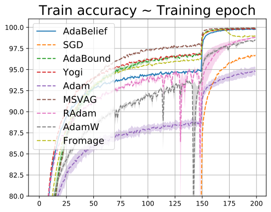
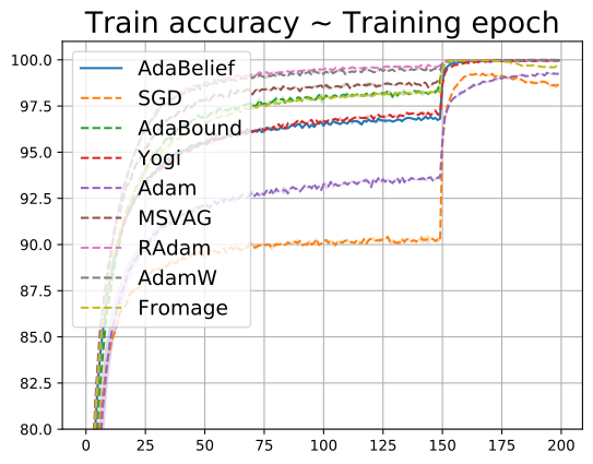
Refer to caption
((a)) VGG11 on Cifar10
Refer to caption
((b)) ResNet34 on Cifar10
Refer to caption
((c)) DenseNet121 on Cifar10
Refer to caption
((d)) VGG11 on Cifar10
Refer to caption
((e)) ResNet34 on Cifar10
Refer to caption
((f)) DenseNet121 on Cifar10
Figure 1: Training (top row) and test (bottom row) accuracy of CNNs on Cifar10 dataset. We report confidence interval [μ±σ]delimited-[]plus-or-minus𝜇𝜎[\mu\pm\sigma] of 3 independent runs.
Refer to caption
((a)) VGG11 on Cifar100
Refer to caption
((b)) ResNet34 on Cifar100
Refer to caption
((c)) DenseNet121 on Cifar100
Refer to caption
((d)) VGG11 on Cifar100
Refer to caption
((e)) ResNet34 on Cifar100
Refer to caption
((f)) DenseNet121 on Cifar100
Figure 2: Training (top row) and test (bottom row) accuracy of CNNs on Cifar10 dataset. We report confidence interval [μ±σ]delimited-[]plus-or-minus𝜇𝜎[\mu\pm\sigma] of 3 independent runs.
Refer to caption
Refer to caption
Figure 3: Training and test accuracy (top-1) of ResNet18 on ImageNet.

2. Image Classification on ImageNet

We experimented with a ResNet18 on ImageNet classication task. For SGD, we use the same learning rate schedule as [30], with an initial learning rate of 0.1, and multiplied by 0.1 at epoch 30 and 60; for AdaBelief, we use an initial learning rate of 0.001, and decayed it at epoch 70 and 80. Weight decay is set as 104superscript10410^{-4} for both cases. To match the settings in [loshchilov2018fixing] and [16], we use decoupled weight decay. As shown in Fig. 3, AdaBelief achieves an accuracy very close to SGD, closing the generalization gap between adaptive methods and SGD. Meanwhile, when trained with a large learning rate (0.1 for SGD, 0.001 for AdaBelief), AdaBelief achieves faster convergence than SGD in the initial phase.
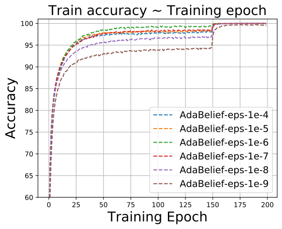
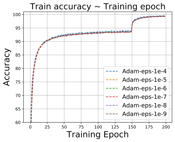
Refer to caption
Refer to caption
Refer to caption
Refer to caption
Figure 4: Training (top row) and test (bottom row) accuracy of ResNet34 on Cifar10, trained with AdaBelief (left column) and Adam (right column) using different values of ϵitalic-ϵ\epsilon. Note that AdaBelief achieves an accuracy above 94%percent9494\% for all ϵitalic-ϵ\epsilon values, while Adam’s accuracy is consistently below 94%percent9494\%.
Refer to caption
Refer to caption
Refer to caption
Refer to caption
Figure 5: Training (top row) and test (bottom row) accuracy of VGG on Cifar10, trained with AdaBelief (left column) and Adam (right column) using different values of learning rate.

3. Robustness to hyperparameters

Robustness to ϵitalic-ϵ\epsilon

We test the performances of AdaBelief and Adam with different values of ϵitalic-ϵ\epsilon varying from 104superscript10410^{-4} to 109superscript10910^{-9} in a log-scale grid. We perform experiments with a ResNet34 on Cifar10 dataset, and summarize the results in Fig. 4. Compared with Adam, AdaBelief is slightly more sensitive to the choice of ϵitalic-ϵ\epsilon, and achieves the highest accuracy at the default valiue ϵ=108italic-ϵsuperscript108\epsilon=10^{-8}; AdaBelief achieves accuracy higher than 94%percent9494\% for all ϵitalic-ϵ\epsilon values, consistently outperforming Adam which achieves an accuracy around 93%percent9393\%.

Robustness to learning rate

We test the performance of AdaBelief with different learning rates. We experiment with a VGG11 network on Cifar10, and display the results in Fig. 5. For a large range of learning rates from 5×1045superscript1045\times 10^{-4} to 3×1033superscript1033\times 10^{-3}, compared with Adam, AdaBelief generates higher test accuracy curve, and is more robust to the change of learning rate.

4. Experiments with LSTM on language modeling

We experiment with LSTM models on Penn-TreeBank dataset, and report the results in Fig. 6. Our experiments are based on this implementation 333https://github.com/salesforce/awd-lstm-lm. Results [μ±σ]delimited-[]plus-or-minus𝜇𝜎[\mu\pm\sigma] are measured across 3 runs with independent initialization. For completeness, we plot both the training and test curves.

We use the default parameters α=0.001,β1=0.9,β2=0.999,ϵ=108formulae-sequence𝛼0.001formulae-sequencesubscript𝛽10.9formulae-sequencesubscript𝛽20.999italic-ϵsuperscript108\alpha=0.001,\beta_{1}=0.9,\beta_{2}=0.999,\epsilon=10^{-8} for 2-layer and 3-layer models; for 1-layer model we set ϵ=1012italic-ϵsuperscript1012\epsilon=10^{-12} and set other parameters as default. For simple models (1-layer LSTM), AdaBelief’s perplexity is very close to other optimizers; on complicated models, AdaBelief achieves a significantly lower perplexity on the test set.
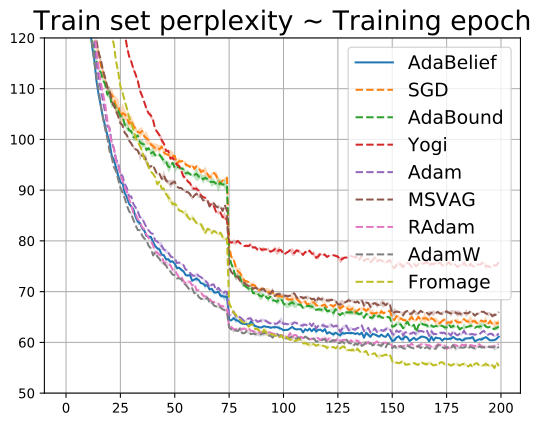
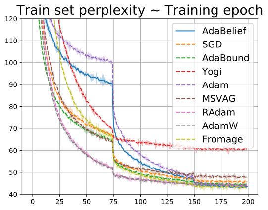
Refer to caption
((a)) 1-layer LSTM
Refer to caption
((b)) 2-layer LSTM
Refer to caption
((c)) 3-layer LSTM
Refer to caption
((d)) 1-layer LSTM
Refer to caption
((e)) 2-layer LSTM
Refer to caption
((f)) 3-layer LSTM
Figure 6: Training (top row) and test (bottom row) perplexity on Penn-TreeBank dataset, lower is better.

5. Experiments with GAN

Table 1: Structure of GAN
Generator Discriminator
ConvTranspose ([inchannel = 100, outchannel = 512, kernel = 4×\times4, stride = 1]) Conv2D([inchannel=3, outchannel=64, kernel = 4×\times4, stride=2])
BN-ReLU LeakyReLU
ConvTranspose ([inchannel = 512, outchannel = 256, kernel = 4×\times4, stride = 2]) Conv2D([inchannel=64, outchannel=128, kernel = 4×\times4, stride=2])
BN-ReLU BN-LeakyReLU
ConvTranspose ([inchannel = 256, outchannel = 128, kernel = 4×\times4, stride = 2]) Conv2D([inchannel=128, outchannel=256, kernel = 4×\times4, stride=2])
BN-ReLU BN-LeakyReLU
ConvTranspose ([inchannel = 128, outchannel = 64, kernel = 4×\times4, stride = 2]) Conv2D([inchannel=256, outchannel=512, kernel = 4×\times4, stride=2])
BN-ReLU BN-LeakyReLU
ConvTranspose ([inchannel = 64, outchannel = 3, kernel = 4×\times4, stride = 2]) Linear(-1, 1)
Tanh

We experimented with a WGAN [21] and WGAN-GP [39]. The code is based on several public github repositories 444https://github.com/pytorch/examples,555https://github.com/eriklindernoren/PyTorch-GAN. We summarize network structure in Table 1. For WGAN, the weight of discriminator is clipped within [0.01,0.01]0.010.01[-0.01,0.01]; for WGAN-GP, the weight for gradient-penalty is set as 10.0, as recommended by the original implementation. For each optimizer, we perform 5 independent runs. We train the model for 100 epochs, generate 64,000 fake samples (60,000 real images in Cifar10), and measure the Frechet Inception Distance (FID) [40] between generated samples and real samples. Our implementation on FID heavily relies on an open-source implementation666https://github.com/mseitzer/pytorch-fid. We report the FID scores in the main paper, and demonstrate fake samples in Fig. 7 and Fig. 8 for WGAN and WGAN-GP respectively.

We also experimented with Spectral Normalization GAN based on a public repository 777https://github.com/POSTECH-CVLab/PyTorch-StudioGAN. For this experiment, we set ϵ=1016italic-ϵsuperscript1016\epsilon=10^{-16} and use the rectification technique as in RAdam. Other hyperparamters and training schemes are the same as in the repository.
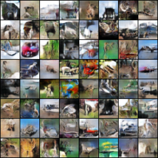
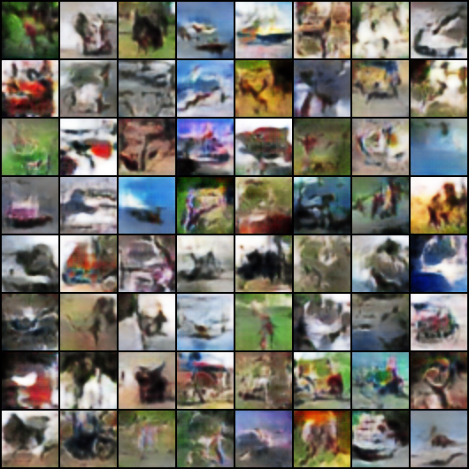
Refer to caption
((a)) AdaBelief
Refer to caption
((b)) RMSProp
Refer to caption
((c)) Adam
Refer to caption
((d)) RAdam
Refer to caption
((e)) Yogi
Refer to caption
((f)) Fromage
Refer to caption
((g)) MSVAG
Refer to caption
((h)) AdaBound
Refer to caption
((i)) SGD
Figure 7: Fake samples from WGAN trained with different optimizers.
Refer to caption
((a)) AdaBelief
Refer to caption
((b)) RMSProp
Refer to caption
((c)) Adam
Refer to caption
((d)) RAdam
Refer to caption
((e)) Yogi
Refer to caption
((f)) Fromage
Refer to caption
((g)) MSVAG
Refer to caption
((h)) AdaBound
Refer to caption
((i)) SGD
Figure 8: Fake samples from WGAN-GP trained with different optimizers.