Independence weights for causal inference with continuous treatments

Abstract

Studying causal effects of continuous treatments is important for gaining a deeper understanding of many interventions, policies, or medications, yet researchers are often left with observational studies for doing so. In the observational setting, confounding is a barrier to the estimation of causal effects. Weighting approaches seek to control for confounding by reweighting samples so that confounders are comparable across different treatment values. Yet, for continuous treatments, weighting methods are highly sensitive to model misspecification. In this paper we elucidate the key property that makes weights effective in estimating causal quantities involving continuous treatments. We show that to eliminate confounding, weights should make treatment and confounders independent on the weighted scale. We develop a measure that characterizes the degree to which a set of weights induces such independence. Further, we propose a new model-free method for weight estimation by optimizing our measure. We study the theoretical properties of our measure and our weights, and prove that our weights can explicitly mitigate treatment-confounder dependence. The empirical effectiveness of our approach is demonstrated in a suite of challenging numerical experiments, where we find that our weights are quite robust and work well under a broad range of settings.
Keywords— Observational Data, Distance Covariance, Confounding, Balancing Weights, Electronic Health Records

1 Introduction

Confounding is a major barrier to studying causal effects of treatments or exposures from observational data. Considerable work has focused on the development of approaches for studying causal effects of binary or otherwise discrete-valued treatments from observational data. With continuous treatments, however, the choices of methods for confounding control are far more limited, and clear guidance that can help practitioners choose among the available methods is lacking. A common approach to reduce confounding by observed variables is using the propensity score, which was initially proposed for binary treatments Rosenbaum and Rubin (1983) and has been generalized to the setting of continuous treatments (Hirano and Imbens, 2004; Imai and Van Dyk, 2004; Zhu et al., 2015; Kennedy et al., 2017; Galvao and Wang, 2015). With binary treatments, the causal effect of interest is often the average treatment effect, which can be estimated as a difference in the weighted averages of the treatment group outcomes, where the weights are proportional to the inverse of the propensity score (Robins et al., 1994, 2000); this method is known as inverse probability weighting (IPW). With continuous treatments, the interest is often in estimation of the causal dose-response functionals (Robins et al., 2000; van der Laan and Robins, 2003) such as the causal average dose-response function (ADRF), which can be estimated using a weighted regression of the outcome on the treatment, where the weights are proportional to the inverse of the conditional density of the treatment given the covariates, the generalized propensity score (GPS).

In the binary treatment setting, IPW estimators can be unstable due to extreme weights and susceptible to model misspecification (Kang and Schafer, 2007; Fan et al., 2021). These issues carry over to IPW estimators for continuous treatments and are substantially more challenging to address. A key reason is that IPW estimation via the GPS requires inverse weighting by a conditional density estimate, not just a conditional probability. Even if the conditional mean of the treatment given covariates is correctly specified, GPS weights can fail to perform well if the distribution of the conditional density is misspecified (Naimi et al., 2014). The difficulty of correctly specifying a conditional distribution is exacerbated with increased dimension of the pre-treatment covariates to be controlled for, i.e., the confounders. The tailored use of flexible machine learning estimation approaches such as that proposed in Zhu et al. (2015) can in many cases yield substantial improvements, however, as shown in our simulations and data analysis, they are still susceptible to the issues of GPS weighting and can perform poorly and/or yield large weights in practice. The ReGPS approach of Colangelo and Lee (2020) directly estimates the inverse GPS without the need for correct specification of a model for the GPS.

As misspecification of a conditional density model can be difficult to diagnose and assess, several works have focused on directly estimating weights to reduce the correlation magnitude between marginal moments of (pre-treatment) covariates and the treatment. Approaches along this line of work include the generalized covariate balancing propensity score (CBPS) approach of Fong et al. (2018) which is an extension of the CBPS approach for discrete treatments (Imai and Ratkovic, 2014), covariate association eliminating weights (Yiu and Su, 2018), and entropy balancing weights (Tübbicke, 2022; Vegetabile et al., 2021). Because these approaches focus on estimation of weights directly as opposed to estimating a conditional density explicitly and inverting it, they tend to be more effective empirically than direct modeling of the GPS. While intuitively appealing, these approaches require careful choices of which moments of both the covariates and the treatment to “decorrelate”. Yet, there is no guidance on specifying the right moments necessary to mitigate bias in estimation of the ADRF due to confounding. Missing important moments can leave substantial residual dependence between the covariates and treatment, see e.g. Figure 1 from our analysis of electronic health record data. Our simulations show that the choice of moments is indeed critically important in practice and that numerical instability can arise when too many moments are used. The tension between including enough moments to reduce bias and the instability of weights as more moments are included can make these methods challenging to use in practice. The general setup of Ai et al. (2021) relies on sieve/series estimators; little finite-sample guidance is provided. Kernel Optimal Orthogonality Weighting (KOW) (Kallus and Santacatterina, 2019) and a generalization of KOW proposed in Martinet (2020) are kernel-based nonparametric extensions of direct weights estimation ideas. They focus on estimating weights to decorrelate over function spaces of treatment and covariates such that there is no need to choose models or which moments to decorrelate. Yet, careful tuning is still required when flexible kernels are used, and, on the other hand, when inflexible kernels are used, there is no guarantee that the resulting weights fully mitigate confounding. Thus, the user is often left with a difficult choice of which kernel to use and unclear guidance on how to choose the kernel’s tuning parameters. Further, no theoretical justification of the approach of Kallus and Santacatterina (2019) is provided. The theoretical results of Martinet (2020) are limited to the convergence of the weighted distribution functions and do not explore properties involving estimation of the ADRF. More extensive discussion of the existing literature can be found in the Section LABEL:supsec:connection_other_methods of the Supplementary Material.

Our work aims to achieve several goals. First, we provide clarity on the role of weights in estimation of the ADRF. To do so, we provide a general decomposition of the error of a weighted nonparametric estimator of the ADRF and demonstrate that, under broad conditions, the ideal weights should induce complete independence between the treatment variable and pre-treatment covariates to guarantee mitigation of confounding bias when estimating the ADRF. While already intuitively understood in the literature, our decomposition precisely quantifies the impact of this dependence on the estimation error in finite samples. We also show that dependence plays a key role in other estimands, such as the causal quantile dose-response function. Second, we develop a measure based on energy statistics (Székely et al., 2007; Székely and Rizzo, 2013) that allows one to assess how well a set of weights is able to induce independence, where smaller values of our measure indicate the weights yield less treatment-covariates dependence and a value of zero indicates complete independence between the treatment and covariates in the weighted data. Huling and Mak (2020) developed a weighted energy distance to mitigate distributional imbalance of covariates in a discrete-treatment setting. In their setting, the energy distance is used to measure distributional imbalance of covariates between different treatment groups, whereas in the setting of this work, a modified distance covariance is used to measure statistical dependence between treatment and confounders. Distributional imbalance plays an important role in confounding control with discrete treatments, but this concept does not naturally generalize to continuous treatments. However, removing statistical dependence between discrete treatments and confounders implies distributional balance has been achieved. As such, our work involves a more general notion of confounding control that can in principle be applied to discrete treatments.

Finally, we propose a new approach for estimating weights, which we call the distance covariance optimal weights (DCOWs), by optimizing our measure. The proposed weights directly aim to mitigate dependence between the treatment and confounders; our error decomposition illustrates that the DCOWs reduce finite sample dependence and thus source of error due to confounding in a weighted nonparametric estimate of the ADRF. In other words, the DCOWs aim to create a pseudo population where treatment and confounders are statistically independent. Our weight construction approach does not require modeling a conditional density, careful tuning of hyperparameters, or choosing which moments of covariates and treatment to decorrelate, making it readily accessible and easy to use for practitioners with varying degrees of statistical sophistication.

We provide some theoretical results for our proposal, showing that our weights indeed reduce dependence between treatment and covariates and fully induce independence asymptotically. Further, we show that with a small penalty on the variability of the weights, our proposal results in the same convergence rate as a nonparametric regression estimate of the ADRF in a scenario with no confounding. Although adding a penalty to reduce weight variability involves the inclusion of a tuning parameter, our proposed approach rarely results in weights with large variability even without penalization. Careful tuning of the parameter that controls weight variability is rarely necessary, as evidenced by our simulation studies, which investigate a wide variety of scenarios with strong and complex confounding and scenarios with moderately high-dimensional confounding, in all of which we fix the tuning parameter to its default value.

Our proposed weights can be used beyond simple weighted nonparametric estimators of the ADRF. Kennedy et al. (2017) and Díaz and van der Laan (2013) extended the idea of doubly-robust estimation to continuous treatments, allowing for estimates that combine outcome regression models (Imbens, 2004; Hill, 2011) and the conditional density models. This allows for relaxed dependence on the correctness of the regression and conditional density models. However, doubly-robust estimators are not immune to highly variable weights and their finite sample performance can suffer if the conditional density model is misspecified. We show that our weights can enhance doubly-robust estimators. Pairing a reasonable outcome regression model with our weights in a doubly-robust fashion can be effective in estimating the ADRF.

The remainder of this paper is organized as follows. We investigate the role of dependence between the treatment and covariates in the estimation of the ADRF in Section 2 and we develop a criterion that assesses how much dependence is mitigated by a set of weights, propose a new weight estimation strategy, and provide some corresponding theory in Section 3. We demonstrate the effectiveness of our approach in finite samples with a suite of challenging simulation studies in Section 4 and illustrate the use of our approach in a real-world study of electronic health record data in Section 5. We conclude the paper with some discussion.

2 Confounding, Weighting, and Dependence

2.1 Setup, notation, and assumptions

The observable quantities we consider consist of the random triplet $({\bf X},A,Y)$, where ${\bf X}\in\mathcal{X}\subseteq\mathbb{R}^{p}$ is a vector of pre-treatment covariates, $A\in\mathcal{A}\subseteq\mathbb{R}$ is a continuous-valued treatment variable indicating the assigned dose for a unit, and $Y\in\mathcal{Y}\subseteq\mathbb{R}$ is an outcome of interest. The variate $({\bf X},A,Y)$ has a joint distribution $F_{{\bf X},A,Y}$ with respect to a dominating measure. We denote the marginal density of the treatment and covariates as $f_{A}(a)$ and $f_{\bf X}({\bf x})$, respectively, the conditional density of the treatment given ${\bf X}$ as $f_{A|{\bf X}}(a|{\bf x})$, and their joint density as $f_{{\bf X},A}(a,{\bf x})$. Similarly, corresponding distribution functions are denoted $F_{A}(a)=\mathbb{P}(A\leq a)$, $F_{\bf X}({\bf x})=\mathbb{P}({\bf X}\leq{\bf x})$, $F_{A|{\bf X}}(a|{\bf x})=\mathbb{P}(A\leq a\>|\>{\bf X}={\bf x})$, and $F_{{\bf X},A}({\bf x},a)=\mathbb{P}({\bf X}\leq{\bf x},A\leq a)$. Our observed data consists of $n$ i.i.d. samples $({\bf X}_{i},A_{i},Y_{i})_{i=1}^{n}$ from $({\bf X},A,Y)$. Note that we drop the subscripts on the density and cumulative distribution functions when there is no ambiguity.

We work under the potential outcomes framework, wherein the potential outcome function $Y(a)$ for $a\in\mathcal{A}$ is the outcome that would be observed if $A$ were set to the value $a$. The causal quantity of interest in this paper is the mean potential outcome function, also called the causal average dose-response function (ADRF), which is $\mu(a)\equiv\mathbb{E}\left[Y(a)\right],\text{ for }a\in\mathcal{A}$.

The causal ADRF $\mu(a)$ can be identified, or expressed in terms of observational data, under standard causal assumptions. These assumptions, which we employ throughout this paper, are 1) consistency, which posits that $A=a$ implies $Y=Y(a)$, 2) positivity, which states that all values of the treatment are possible across the covariate space in the sense that $f(a|{\bf X}={\bf x})\geq\nu>0$ for all ${\bf x}\in\mathcal{X}$ for some constant $\nu$, and 3) ignorability of the assignment mechanism: $Y(a){\perp\!\!\!\perp}A\>|\>{\bf X}$ for all $a\in\mathcal{A}$, where ${\perp\!\!\!\perp}$ denotes (conditional) independence. Under assumptions 1)-3), the dose-response function is identified as $\mu(a)=\mathbb{E}_{\bf X}\left(\mathbb{E}\left[Y\>|\>{\bf X},A=a\right]\right)=\mathbb{E}_{\bf X}\left[\mu({\bf X},a)\right]$. Estimation of the dose-response function via regression-based estimation of the mean function $\mu({\bf X},a)\equiv\mathbb{E}\left[Y\>|\>{\bf X},A=a\right]$, however, can be highly challenging. Misspecification of the regression function can result in poor estimation of $\mu(a)$, and nonparametric estimation of the regression function is also difficult, especially when ${\bf X}$ is not low dimensional. Instead, this paper focuses on weighting-based estimators of $\mu(a)$. A benefit of weighting estimators is that the dose-response function can be flexibly estimated by univariate (weighted) nonparametric regression, whereas with regression-based estimation, the need to incorporate covariates in a regression may make flexible estimation of the ADRF more difficult due to the additional dimensions. A conceptual benefit of weighting methods over regression-based methods is that they provide a clear separation between design and analysis phases of a study. This separation is critical when substantial or iterative model-building is required to control for confounding.

2.2 Ignorability, independence, and the GPS

To reliably estimate the causal dose response function using observational data, sources of structural bias should be mitigated, among which the bias due to confounding is the most common. Consider the setting where the covariate vector ${\bf X}$ contains all confounders in studying the causal relationship between $A$ and $Y$. Blocking the backdoor path $A\leftarrow{\bf X}\rightarrow Y$ mitigates confounding. One way of blocking the backdoor path is by removing the arrow between $A$ and ${\bf X}$ (i.e., making $A$ independent of ${\bf X}$). In a randomized trial, the independence between $A$ and ${\bf X}$ holds due to randomization. This motivates us to create a pseudo-population mimicking the one we would observe under such a trial by reweighting the subjects in an observational study such that $A$ is independent of ${\bf X}$ in the pseudo-population. Weighting by the generalized propensity score $f_{A|{\bf X}}(A\>|\>{\bf X})$ (GPS) (Hirano and Imbens, 2004) achieves such and extends the pioneering work of Rosenbaum and Rubin (1983) for binary treatments to continuous treatments.

For continuous treatments, stabilized GPS weights are computed as $f_{A}(A)/f_{A|{\bf X}}(A\>|\>{\bf X})$ (Robins et al., 2000), which naturally arise in estimating equations for the dose-response function via semiparametric theory (Kennedy et al., 2017). Estimating the weights requires correct specification not only of the mean of the conditional density of the treatment, but also of its higher order properties such as shape. When any of these is misspecified, bias can result in estimates of the ADRF (Naimi et al., 2014; Zhu et al., 2015), indicating a particularly sensitive reliance on correct modeling of the conditional distribution of the treatment given the covariates. Furthermore, similar to standard propensity score weights, GPS modeling can yield extreme weights, leading to unstable estimation. Weight trimming/capping may alleviate the problem of large weights but can be seen as ad hoc and may change the estimand (Crump et al., 2009): the estimated ADRF will correspond to the population represented by the newly weighted sample rather than to the original target population.

The stabilized GPS weights $f_{A}(A)/f_{A|{\bf X}}(A\>|\>{\bf X})$ have several key properties that have motivated work to improve upon the GPS weights. Namely, when weighting by the GPS weights in the population sense, they 1) result in independence of ${\bf X}$ and $A$, 2) preserve the marginal distributions of ${\bf X}$ and $A$, and 3) have mean 1. These properties are listed more explicitly in Section LABEL:sec:appendix_aa of the Supplementary Material. Instead of indirectly estimating the weights by estimating the GPS, a nascent line of work has involved methods which directly estimate weights designed to satisfy the above three properties via balancing criteria. For example, work has focused on estimation of weights that induce zero marginal correlation between treatment and covariates (Fong et al., 2018; Yiu and Su, 2018; Vegetabile et al., 2021). Although they are more robust than GPS weights, these approaches rely on both the correct choice of moments of the covariates and the choice of moments of the treatment variable to decorrelate. Yet, there is little guidance in deciding which set of moments in both covariates and treatment to focus on, as these choices depend on the form of the true potential outcome-generating model.

The aforementioned three properties of GPS weights are intuitively appealing, but it is not immediately clear which of or in what manner these properties are important in mitigating bias in a weighted nonparametric estimator of the ADRF. To justify which properties are crucial in weights estimation, we derive the relationship between the properties of weighted dose-response function estimators using generic weights and the systematic source of error of the weighted estimator for the ADRF. We demonstrate that the ability of a set of weights to induce independence between ${\bf X}$ and $A$ is critical for reducing the bias of a weighted estimator.

2.3 A general error decomposition for weighted nonparametric estimators of the ADRF

In this section we aim to provide an explicit mechanistic connection between dependence and bias in weighted estimates of the ADRF. Although it is understood that using weights constructed from a well-estimated conditional density is consistent (Kennedy et al., 2017), it is unclear what role weights play more generally. It is not immediately clear what the connection is between the balancing criteria that aim to “decorrelate” moments of covariates and moments of the treatment variable and the systematic bias in estimating the ADRF. In the following, we investigate the precise source of the systematic bias of an estimator and illuminate the role of the weights in influencing the bias. We focus on weighted Nadaraya-Watson estimators of the ADRF for clarity of presentation, though the key message applies to weighted local polynomial regression and other weighted nonparametric regression.

The response can be expressed as $Y_{i}=\mu({\bf X}_{i},A_{i})+\varepsilon_{i}$, where $\varepsilon_{i}\equiv Y_{i}(A_{i})-\mu({\bf X}_{i},A_{i})$. By construction, $\varepsilon_{i}$ have mean zero but are not necessarily identically distributed. Given any set of weights ${\bf w}=(w_{1},\dots,w_{n})$ and a kernel $K_{h}(A_{i}-a_{0})=K(\frac{A_{i}-a_{0}}{h})/h$ centered at $A=a_{0}$ with bandwidth $h>0$, the weighted Nadaraya-Watson (NW) estimator of the ADRF at $A=a_{0}$ is

$$\widehat{\mu}_{NW}^{{\bf w}}(a_{0})=\frac{\sum_{i=1}^{n}Y_{i}w_{i}K_{h}(A_{i}-a_{0})}{\sum_{i=1}^{n}K_{h}(A_{i}-a_{0})}.$$ (1)

This class of estimators of the causal ADRF is motivated by the identification results of Colangelo and Lee (2020), who showed under certain causal conditions and assumptions regarding the kernel $K_{h}$ that $\mu(a_{0})=\lim_{h\to 0}\mathbb{E}\left[YK_{h}(A-a_{0})/f_{A|{\bf X}}(a_{0}\mid{\bf X})\right]$, which implies the use of the inverse of $f_{A|{\bf X}}(A\mid{\bf X})$ as weights, since $\mu(a_{0})=\lim_{h\to 0}\mathbb{E}\left[YK_{h}(A-a_{0})w^{*}({\bf X},A)\right]/\mathbb{E}\left[K_{h}(A-a_{0})\right]=\lim_{h\to 0}\mathbb{E}\left[YK_{h}(A-a_{0})w^{*}({\bf X},a_{0})\right]/f_{A}(a_{0})$, where $w^{*}({\bf x},a)=f_{A}(a)/f_{A|{\bf X}}(a\mid{\bf X}={\bf x})$. Given any weights ${\bf w}$, the error of (1) at $A=a_{0}$ can be decomposed as

$$\widehat{\mu}_{NW}^{{\bf w}}(a_{0})-\mu(a_{0})={} \int_{\mathcal{X}}\int_{\mathcal{A}}\mu({\bf x},a_{0})\mathrm{d}\left[F^{n}_{{\bf X},A,{\bf w}}-F^{n}_{{\bf X}}F^{n}_{A}\right]({\bf x},a)$$ (2)

$$+\int_{\mathcal{X}}\mu({\bf x},a_{0})\mathrm{d}\left[F^{n}_{{\bf X}}-F_{\bf X}\right]({\bf x})+\left(\frac{f_{A}(a_{0})}{\widehat{f}^{n}_{A,h}(a_{0})}-1\right)\int_{\mathcal{X}}\mu({\bf x},a_{0})\mathrm{d}F^{n}_{{\bf X}}({\bf x})$$

$$+\left(\frac{f_{A}(a_{0})}{\widehat{f}^{n}_{A,h}(a_{0})}-1\right)\int_{\mathcal{X}}\int_{\mathcal{A}}\mu({\bf x},a_{0})\mathrm{d}\left[F^{n}_{{\bf X},A,{\bf w}}-F^{n}_{{\bf X}}F^{n}_{A}\right]({\bf x},a)$$

$$+{\widehat{f}^{n}{}}^{-1}_{A,h}(a_{0})\int_{\mathcal{X}}\int_{\mathcal{A}}\left[\mu({\bf x},a)K_{h}(a-a_{0})-\mu({\bf x},a_{0})f_{A}(a_{0})\right]\mathrm{d}F^{n}_{{\bf X},A,{\bf w}}({\bf x},a)$$

$$+\frac{1}{n}\sum_{i=1}^{n}\varepsilon_{i}w_{i}{\widehat{f}^{n}{}}^{-1}_{A,h}(a_{0}){K_{h}(A_{i}-a_{0})},$$ (3)

where $\widehat{f}^{n}_{A,h}(a_{0})=\int_{\mathcal{A}}K_{h}(a-a_{0})\mathrm{d}F^{n}_{A}(a)$ is a kernel density estimate of $f_{A}(a_{0})$, $F^{n}_{{\bf X}}({\bf x})=\\ n^{-1}\sum_{i=1}^{n}I({\bf X}_{i}\leq{\bf x})$ is the empirical cumulative distribution function (CDF) of $\{{\bf X}_{i}\}_{i=1}^{n}$, $F^{n}_{A}(a)=n^{-1}\sum_{i=1}^{n}I(A_{i}\leq a)$ is the empirical CDF of $\{A_{i}\}_{i=1}^{n}$, and $F^{n}_{{\bf X},A,{\bf w}}({\bf x},a)=n^{-1}\sum_{i=1}^{n}w_{i}I({\bf X}_{i}\leq{\bf x},A_{i}\leq a)$ is the weighted empirical CDF of $\{{\bf X}_{i},A_{i}\}_{i=1}^{n}$ using weights ${\bf w}$. We provide a derivation of this decomposition in Section LABEL:sec:appendix_b of the Supplementary Material. The second term on the right is due to sampling variability only and has mean zero and converges at rate $n^{-1/2}$ if the sample is representative of the super-population. The expectations of the third, fourth, and fifth terms on the right above go to 0 when $h\to 0$ regardless of the weights ${\bf w}$. The last term has mean zero regardless of both the weights and the bandwidth, though its variability is impacted by the weights. We note, however, that the third through fifth terms are not guaranteed to converge to zero without additional conditions on the variability of the weights.

On the other hand, the first term (2) on the right above is the source of systematic bias of the weighted estimator unrelated to kernel smoothing. In other words, taking limits of the bandwidth of the kernel to 0 and sample size to infinity does not make (2) vanish. This term also provides insight into why using the weights we propose later performs well in finite sample settings when used in treatment effect estimators, as targeting this term can help decrease the magnitude of the systematic component of the bias of an estimator. If a given set of weights induces finite-sample independence of ${\bf X}$ and $A$ in the sense that $F^{n}_{{\bf X},A,{\bf w}}({\bf x},a)=F^{n}_{{\bf X}}({\bf x})F^{n}_{A}(a)$ for all ${\bf x}\in\mathcal{X}$, $a\in\mathcal{A}$, then the source of bias (2) of $\hat{\mu}^{{\bf w}}(a_{0})$ will be zero. The mean-squared error of the estimator will, however, depend primarily on both the bias term (2) and the variance of (3). Mitigating the variance of (3) merely amounts to controlling the squares of the weights; however, providing a measure that can characterize (2) is non-trivial and none exists in the literature. The term (2) is bounded by the distance between $F^{n}_{{\bf X},A,{\bf w}}({\bf x},a)$ and $F^{n}_{{\bf X}}({\bf x})F^{n}_{A}(a)$ provided that $\mu({\bf x},a_{0})$ is bounded. Without modeling the response function, constructing a measure that bounds (2) is critical for assessing a set of weights.

Remark 1.

The role of weights in their ability to induce independence between treatment and covariates is not unique to estimation of the ADRF and applies to a wide variety of estimands. Consider estimation of the causal dose-response quantile function $q_{Y(a_{0})}(\alpha)=\inf\{y:F_{Y(a_{0})}(y)\leq\alpha\}$, where $F_{Y(a_{0})}(y)=\mathbb{P}(Y(a_{0})\leq y)=\mathbb{E}_{{\bf X}}\left\{\mathbb{P}(Y\leq y|{\bf X},A=a_{0})\right\}=\mathbb{E}_{{\bf X}}\left\{F_{Y|{\bf X},A}(y|{\bf X},A=a_{0})\right\}$. By replacing $Y_{i}$ with $I(Y_{i}\leq y)$ in (1), we can show that the estimation error of $F_{Y(a_{0})}(y)$ also depends on how well weights mitigate dependence between $A$ and ${\bf X}$. More details are included in Section LABEL:sec:appendix_b of the Supplementary Material.

In practice, the estimator $\widehat{\mu}_{NW}^{{\bf w}}(a_{0})$ in (1) may be unstable, as the weights only appear in the numerator, so the estimated ADRF may lie outside the range of the observed values of the response. Instead, a more stable estimator is the following weighted average of the responses

$$\widehat{\mu}_{NWs}^{{\bf w}}(a_{0})=\frac{\sum_{i=1}^{n}Y_{i}w_{i}K_{h}(A_{i}-a_{0})}{\sum_{i=1}^{n}w_{i}K_{h}(A_{i}-a_{0})},$$ (4)

which can be viewed as the minimizer of a weighted least squares problem where the $i$th weight is $w_{i}K_{h}(A_{i}-a_{0})$. The estimator (4) is also a valid estimator of the ADRF as long as the denominator divided by $\sum_{i=1}^{n}w_{i}$ is a consistent estimator of $f_{A}(a_{0})$; in this case the key source of systematic bias still depends on the term (2).

3 Measuring and Controlling Weighted Dependence with Energy Statistics

3.1 A criterion to evaluate the quality of a set of weights

Having established the relationship between the dependence of $A$ and ${\bf X}$ and the error in a weighted nonparametric estimate of the ADRF, we now construct a criterion that can assess how well a given set of weights induces independence on the weighted scale, i.e., we aim to characterize and bound the distance between $F^{n}_{{\bf X},A,{\bf w}}$ and $F^{n}_{{\bf X}}F^{n}_{A}$. We do so by building on the ideas of distance covariance (Székely et al., 2007), which is a measure of dependence between two random vectors of arbitrary but dimensions. The population distance covariance is zero if and only if the vectors are independent. Hence, a weighted distance covariance will be a useful component for our measure. Let ${\bf w}=(w_{1},\dots,w_{n})$ and define the weighted distance covariance to be

$$\mathcal{V}^{2}_{n,{\bf w}}({\bf X},A)=\frac{1}{n^{2}}\sum_{k,\ell=1}^{n}w_{k}w_{\ell}C_{k\ell}D_{k\ell},$$ (5)

where

$$c_{k\ell} =\lVert{\bf X}_{k}-{\bf X}_{\ell}\rVert_{2},\quad\mkern 1.5mu\overline{\mkern-1.5muc\mkern-1.5mu}\mkern 1.5mu_{k\cdot} =\frac{1}{n}\sum_{\ell=1}^{n}c_{k\ell},\quad\mkern 1.5mu\overline{\mkern-1.5muc\mkern-1.5mu}\mkern 1.5mu_{\cdot\ell}=\frac{1}{n}\sum_{k=1}^{n}c_{k\ell},$$

$$\mkern 1.5mu\overline{\mkern-1.5muc\mkern-1.5mu}\mkern 1.5mu_{\cdot\cdot} =\frac{1}{n^{2}}\sum_{k,\ell=1}^{n}c_{k\ell},\quad C_{k\ell} =c_{k\ell}-\mkern 1.5mu\overline{\mkern-1.5muc\mkern-1.5mu}\mkern 1.5mu_{k\cdot}-\mkern 1.5mu\overline{\mkern-1.5muc\mkern-1.5mu}\mkern 1.5mu_{\cdot\ell}+\mkern 1.5mu\overline{\mkern-1.5muc\mkern-1.5mu}\mkern 1.5mu_{\cdot\cdot},$$

for $k,\ell=1,\dots,n$. Similarly define $d_{k\ell}=\lvert A_{k}-A_{\ell}\rvert$, $\mkern 1.5mu\overline{\mkern-1.5mud\mkern-1.5mu}\mkern 1.5mu_{k\cdot}=\frac{1}{n}\sum_{\ell=1}^{n}d_{k\ell}$, $\mkern 1.5mu\overline{\mkern-1.5mud\mkern-1.5mu}\mkern 1.5mu_{\cdot\ell}=\frac{1}{n}\sum_{k=1}^{n}d_{k\ell}$, and $D_{k\ell}=d_{k\ell}-\mkern 1.5mu\overline{\mkern-1.5mud\mkern-1.5mu}\mkern 1.5mu_{k\cdot}-\mkern 1.5mu\overline{\mkern-1.5mud\mkern-1.5mu}\mkern 1.5mu_{\cdot\ell}+\mkern 1.5mu\overline{\mkern-1.5mud\mkern-1.5mu}\mkern 1.5mu_{\cdot\cdot}$. The quantity (5) simplifies to the original distance covariance when weights are all $1$. Since the original distance covariance is always non-zero, (5) is also always non-zero if the weights are positive. We now provide further insight and motivation of the form of $\mathcal{V}^{2}_{n,{\bf w}}({\bf X},A)$ and its interpretation in terms of weighted distributions.

Letting $i=\sqrt{-1}$, we define the (weighted) empirical characteristic functions as $\varphi^{n}_{{\bf X},A,{\bf w}}({\bf t},s)=$ $\frac{1}{n}\sum_{j=1}^{n}w_{j}\exp\{i\mathbf{t}^{{\sf\scriptscriptstyle{T}}}{{\bf X}}_{j}+isA_{j}\}$, $\varphi^{n}_{{\bf X},{\bf w}}({\bf t})=$ $\frac{1}{n}\sum_{j=1}^{n}w_{j}\exp\{i\mathbf{t}^{{\sf\scriptscriptstyle{T}}}{{\bf X}}_{j}\}$, $\varphi^{n}_{A,{\bf w}}(s)=\frac{1}{n}\sum_{j=1}^{n}w_{j}\exp\{isA_{j}\}$, and empirical characteristic functions $\varphi^{n}_{{\bf X},A}({\bf t},s)$, $\varphi^{n}_{{\bf X}}({\bf t})$ and $\varphi^{n}_{A}(s)$ are defined accordingly.

Theorem 3.1.

Let ${\bf w}=(w_{1},\dots,w_{n})$ be a vector of weights such that $\sum_{i=1}^{n}w_{i}=n$ and $w_{i}\geq 0$ for all $i=1,\dots,n$. Then $\mathcal{V}^{2}_{n,{\bf w}}({\bf X},A)\geq 0$ and

$$\mathcal{V}^{2}_{n,{\bf w}}({\bf X},A)={} \int_{\mathbb{R}^{p+1}}|\varphi^{n}_{{\bf X},A,{\bf w}}({\bf t},s)-\varphi^{n}_{{\bf X},{\bf w}}({\bf t})\varphi^{n}_{A,{\bf w}}(s)$$

$$\;\;\quad\quad+(\varphi^{n}_{{\bf X},{\bf w}}({\bf t})-\varphi^{n}_{{\bf X}}({\bf t}))(\varphi^{n}_{A,{\bf w}}(s)-\varphi^{n}_{A}(s))|^{2}\omega({\bf t},s)\mathrm{d}{\bf t}\;\mathrm{d}s$$ (6)

where $\omega({\bf t},s)=(c_{p}c_{1}\lVert{\bf t}\rVert_{2}^{1+p}|s|^{2})^{-1}$ with $c_{d}=\frac{\pi^{(1+d)/2}}{\Gamma((1+d)/2)}$, and $\Gamma(\cdot)$ is the complete gamma function.

Based on (6), it is clear that if $F^{n}_{{\bf X},A,{\bf w}}=F^{n}_{{\bf X}}F^{n}_{A}$, then $\mathcal{V}^{2}_{n,{\bf w}}({\bf X},A)=0$. However, the converse is not necessarily true. Yet, if the weights preserve the marginal distribution of treatment and covariates, i.e. $F^{n}_{{\bf X},{\bf w}}=F^{n}_{{\bf X}}$ and $F^{n}_{A,{\bf w}}=F^{n}_{A}$, then $\mathcal{V}^{2}_{n,{\bf w}}({\bf X},A)=0$ implies that $F^{n}_{{\bf X},A,{\bf w}}=F^{n}_{{\bf X}}F^{n}_{A}$. In other words, if one can add additional terms to (5) that also measure the distance between $F^{n}_{{\bf X},{\bf w}}$ and $F^{n}_{{\bf X}}$ along with that between $F^{n}_{A,{\bf w}}$ and $F^{n}_{A}$, then (5) can be utilized to construct a measure that determines the distance between $F^{n}_{{\bf X},A,{\bf w}}$ and $F^{n}_{{\bf X}}F^{n}_{A}$, i.e., a measure for the weighted dependence between ${\bf X}$ and $A$. We leverage the weighted energy distance proposed in Huling and Mak (2020) to help construct such a measure.

Applied to our setting, the weighted energy distance between $F^{n}_{{\bf X},{\bf w}}$ and $F^{n}_{\bf X}$ is

$$\quad\mathcal{E}(F^{n}_{{\bf X},{\bf w}},F^{n}_{{\bf X}})\equiv{} \frac{2}{n^{2}}\sum_{i=1}^{n}\sum_{j=1}^{n}w_{i}\lVert{{\bf X}}_{i}-{{\bf X}}_{j}\rVert_{2}-\frac{1}{n^{2}}\sum_{i=1}^{n}\sum_{j=1}^{n}w_{i}w_{j}\lVert{{\bf X}}_{i}-{{\bf X}}_{j}\rVert_{2}-\frac{1}{n^{2}}\sum_{i=1}^{n}\sum_{j=1}^{n}\lVert{{\bf X}}_{i}-{{\bf X}}_{j}\rVert_{2}.$$

Due to Proposition 1 of Huling and Mak (2020), it can be shown that $\mathcal{E}(F^{n}_{{\bf X},{\bf w}},F^{n}_{{\bf X}})=\int_{\mathbb{R}^{p}}|\varphi^{n}_{\bf X}({\bf t})-\varphi^{n}_{{\bf X},{\bf w}}({\bf t})|^{2}\omega(\mathbf{t})\mathrm{d}\mathbf{t}$, where $\omega(\mathbf{t})=1/(C_{p}\lVert{\bf t}\rVert_{2}|^{1+p})$, $C_{p}=\pi^{(1+p)/2}/\Gamma((1+p)/2)$ is a constant. The weighted energy distance $\mathcal{E}(F^{n}_{A,{\bf w}},F^{n}_{A})$ between $F^{n}_{A,{\bf w}}$ and $F^{n}_{A}$ can be similarly defined.

Our proposed measure of the level of independence induced by a set of weights is defined as

$${\cal D}({\bf w})=\mathcal{V}^{2}_{n,{\bf w}}({\bf X},A)+\mathcal{E}(F^{n}_{{\bf X},{\bf w}},F^{n}_{{\bf X}})+\mathcal{E}(F^{n}_{A,{\bf w}},F^{n}_{A}).$$ (7)

The following result demonstrates that ${\cal D}({\bf w})$ indeed achieves its stated goal.

Theorem 3.2.

Let ${\bf w}=(w_{1},\dots,w_{n})$ be such that $w_{i}>0$ and $\sum_{i=1}^{n}w_{i}=n$. Then ${\cal D}({\bf w})\geq 0$ with equality to zero if and only if $\varphi^{n}_{{\bf X},A,{\bf w}}({\bf t},s)=\varphi^{n}_{{\bf X}}({\bf t})\varphi^{n}_{A}(s)$, $\varphi^{n}_{{\bf X},{\bf w}}({\bf t})=\varphi^{n}_{{\bf X}}({\bf t})$, and $\varphi^{n}_{A,{\bf w}}(s)=\varphi^{n}_{A}(s)$ for all $({\bf t},s)\in\mathbb{R}^{p+1}$. Further, $\int|\varphi^{n}_{{\bf X},A,{\bf w}}({\bf t},s)-\varphi^{n}_{{\bf X}}({\bf t})\varphi^{n}_{A}(s)|^{2}\omega({\bf t},s)\mathrm{d}{\bf t}\mathrm{d}s\leq 3{\cal D}({\bf w})$.

Thus, smaller values of ${\cal D}({\bf w})$ indicate smaller potential for dependence between ${\bf X}$ and $A$ after weighting and better preservation of the marginal distributions, and larger values indicate the opposite. ${\cal D}({\bf w})=0$ implies the weights induce complete independence between ${\bf X}$ and $A$ and that the marginal distributions of ${\bf X}$ and $A$ are exactly preserved.

We also have the following result, which shows how the proposed distance acts as a bound on integration errors over a class of functions.

Lemma 3.3.

Let $\mathcal{H}$ be the native space induced by the radial kernel $\Phi(\cdot,\cdot)=-\|\cdot\|_{2}\times-|\cdot|$ on $\mathcal{X}\times\mathcal{A}$ equipped with inner product $\langle\cdot,\cdot\rangle_{\mathcal{H}}$ and norm $\|g\|_{\mathcal{H}}=\sqrt{\langle g,g\rangle_{\mathcal{H}}}$ for any $g(\cdot,\cdot)\in\mathcal{H}=\mathcal{H}_{\mathcal{X}}\otimes\mathcal{H}_{\mathcal{A}}$, where $\mathcal{H}_{\mathcal{X}},\mathcal{H}_{\mathcal{A}}$ are defined in Theorem 4 of Mak and Joseph (2018). Then, for any weights ${\bf w}$ satisfying $\sum_{i=1}^{n}w_{i}=n,w_{i}\geq 0$, we have

$$\left[\int_{\mathcal{X}}\int_{\mathcal{A}}g({\bf x},a)\mathrm{d}\left[F^{n}_{{\bf X},A,{\bf w}}-F^{n}_{\bf X}F^{n}_{A}\right]({\bf x},a)\right]^{2}\leq C_{g}\mathcal{D}({\bf w}),$$ (8)

where $C_{g}=3\|g\|^{2}_{\mathcal{H}}\geq 0$ is a constant depending on only $g$.

For any $a\in\mathcal{A}$ if $\mu(\cdot,a)\in\mathcal{H}_{\mathcal{X}}$, we can see that ${\cal D}({\bf w})$, modulo a constant, acts as a bound on the systematic bias term (2) as long as $\mu(\cdot,a)$ is sufficiently smooth. Thus, if $\mu({\bf x},a)$ is contained in $\mathcal{H}$, then we can expect weights with smaller ${\cal D}({\bf w})$ to lead to smaller systematic bias. The space $\mathcal{H}$ is a reasonably broad class of functions as it contains the Sobolev space of functions with square-integrable functions with $r<\lceil(p+1)/2\rceil$-th differentials (Mak and Joseph, 2018; Huling and Mak, 2020). Our goal for the next section is to define weights that are optimal in terms of our criterion. The weights that minimize ${\cal D}({\bf w})$ will result in mitigation of the dependence of ${\bf X}$ and $A$ induced by nonrandom selection into treatment.

In contrast to the measure (7) comprised of the distance covariance term (6), it is natural to wonder whether it would instead be more appropriate to simply define a distance as $\int|\varphi^{n}_{{\bf X},A,{\bf w}}({\bf t},s)-\varphi^{n}_{{\bf X}}({\bf t})\varphi^{n}_{A}(s)|^{2}\omega({\bf t},s)\mathrm{d}{\bf t}\mathrm{d}s$ and construct a relationship between this distance and Euclidean norms computable from data. However, we have found that the resulting quantity can be empirically problematic and unreliable. Further, we have found that optimization of such a quantity cannot be achieved reliably by existing algorithms and is thus not suitable for the proactive construction of weights. Our proposed quantity, while more complicated, does not exhibit any of these issues in the sense that it reliably measures dependence, and, as we will demonstrate, it is straightforward to optimize with existing quadratic programming software.

3.2 A new proposal: distance covariance optimal independence weights

We define the distance covariance optimal weights (DCOWs) to be

$${\bf w}^{d}_{n}\in{} \operatorname*{argmin}_{{\bf w}=(w_{1},\dots,w_{n})}{\cal D}({\bf w})\text{ such that }\sum_{i=1}^{n}w_{i}=n,\text{ and }w_{i}\geq 0\text{ for }i=1,\dots,n.$$ (9)

The name reflects that the weights are constructed as the optimizers of our distance-covariance-based criterion. Due to Theorem 3.2, the DCOWs ${\bf w}^{d}_{n}$ are designed to minimize dependence between ${\bf X}$ and $A$ on the weighted scale while keeping the weighted marginal distributions of ${\bf X}$ and $A$ close to those of the unweighted data. The constraint $\sum_{i=1}^{n}w_{i}=n$ ensures that $F^{n}_{{\bf X},A,{{\bf w}^{d}_{n}}}$ is a valid distribution function. Since ${\cal D}({\bf w})$ tracks with the dependence induced by a set of weights, the DCOWs can be thought of as optimal independence weights (i.e., optimal with respect to achieving independence between the treatment and covariates).

Although, as we will show later, the DCOWs result in consistent weighted dose-response estimators, they may not guarantee optimal convergence rates without additional constraints. Instead, a small change to our criterion to include penalization of the squares of the weights provides control of the variability of the weights without sacrificing their bias-reduction property. This additional penalty is akin to focusing more directly on mean squared error instead of bias and can be interpreted as discouraging the effective sample size (ESS) after weighting from being too small. In particular, the ESS is typically approximated as $(\sum_{i}w_{i})^{2}/\sum_{i}w_{i}^{2}$ (Kish, 1965), which, due to our constraints, is $n^{2}/\sum_{i}w_{i}^{2}$ and is precisely the inverse of our proposed penalty. Further, combining a “balance” criterion with a means of weight variability mitigation is in line with the recommendations of Chattopadhyay et al. (2020).

We now define the penalized distance covariance optimal weights (PDCOWs) to be

$${\bf w}^{pd}_{n}\in{} \operatorname*{argmin}_{{\bf w}=(w_{1},\dots,w_{n})}{\cal D}({\bf w})+\lambda\frac{1}{n^{2}}\sum_{i=1}^{n}w_{i}^{2}$$

$$\text{ such that }\sum_{i=1}^{n}w_{i}=n,w_{i}\geq 0\text{ for }0<\lambda<\infty,i=1,\dots,n.$$ (10)

Here, the tuning parameter $\lambda$ is any positive constant and can be chosen by the user to achieve a desired ESS. A lemma provided in Section LABEL:supsec:more_theory of the Supplementary Material similar to Lemma 3.3 shows that the penalized version of our criterion acts as a bound on the term in the left-hand side of (8) plus the squares of the weights, which is more akin to a bound on the root mean squared error than bias as in Lemma 3.3. Although having a non-zero, positive value of $\lambda$ is necessary for the convergence rate guarantee of Theorem 3.5, in practice we have found that minimal or even no penalization at all works well because the unpenalized weights, the DCOWs, tend to be quite stable. In all analyses described later, we use only the DCOWs with no weight penalization.

Both the DCOWs and PDCOWs can be used in a wide variety of estimators for various causal estimands involving continuous treatments, not just Nadaraya-Watson-based estimators and not just estimators of the ADRF. The weights can be used either in a simple weighted nonparametric estimator of the dose-response function or to supplement any doubly-robust estimator of such. For the former, our weights provide a fully nonparametric and empirically robust estimation approach that requires only mild moment conditions on the covariates and treatment for estimation consistency. For the latter, such an estimator using our weights is guaranteed to be consistent regardless of the correctness of the outcome model, while it still enjoys efficiency gains if the outcome model is well-specified.

Remark 2.

The optimization problems (9) and (10) can be formulated as quadratic programming problems with linear constraints, making them straightforward to implement with commercial and open-source solvers such as OSQP (Stellato et al., 2020). If in practice additional emphasis on correlations of particular moments of covariates and the treatment is of importance, our framework can accommodate that by adding additional linear constraints. The details are deferred to Sections LABEL:sec:computation and LABEL:sec:extensions of the Supplementary Material.

In a later section, we provide more formal statements on the consistency of dose-response function estimators that use our proposed distance covariance optimal weights.

3.3 Asymptotic properties

We first show that the distance covariance optimal weights do induce complete independence asymptotically. Throughout this section we define $w^{*}({\bf x},a)=f_{A}(a)/f_{A|{\bf X}}(a|{\bf X}={\bf x})$ to be the “true” normalized density weights.

Theorem 3.4.

Let ${\bf w}^{d}_{n}$ be the distance covariance optimal weights defined in (9). Then if $\mathbb{E}\lVert{\bf X}\rVert_{2}<\infty$ and $\mathbb{E}\lvert A\rvert<\infty$ we have

$$\lim_{n\to\infty}F^{n}_{{\bf X},A,{\bf w}^{d}}({\bf x},a)=F_{{\bf X}}({\bf x})F_{A}(a)$$ (11)

almost surely for every continuity point $({\bf x},a)\in\mathbb{R}^{p+1}$ and further that $\lim_{n\to\infty}F^{n}_{{\bf X},{\bf w}^{d}}({\bf x})=F_{{\bf X}}({\bf x})$ for every continuity point ${\bf x}\in\mathbb{R}^{p}$ and $\lim_{n\to\infty}F^{n}_{A,{\bf w}^{d}}({\bf x},a)=F_{A}(a)$ for every continuity point $a\in\mathbb{R}$. If, additionally $\mathbb{E}{w^{*}}^{2}({\bf X},A)<\infty$ holds, then the same result holds for ${\bf w}^{pd}$.

Theorem 3.4 is in some sense the most important property of the DCOWs, as it demonstrates the feasibility of using these weights not just in estimation of the ADRF, but also in the estimation of many causal estimands that require independence. In particular, if the source of confounding bias has the form $\int_{\mathcal{X}}\int_{\mathcal{A}}g({\bf x},a)\mathrm{d}\left[F^{n}_{{\bf X},A,{\bf w}}-F^{n}_{{\bf X}}F^{n}_{A}\right]({\bf x},a)$ for some function $g\in\mathcal{H}$, then the use of our weights can be justified due to Lemma 3.3 and Theorem 3.4.

We now show that for the particular task of estimating the ADRF, using the DCOWs in a weighted Nadaraya-Watson estimator results in consistent estimation of the ADRF.

Theorem 3.5.

Assume that the kernel $K(\cdot)$ is symmetric, second order, i.e. it meets the conditions that $\int uK(u)\mathrm{d}u=0$, $\int K(u)\mathrm{d}u=1$, and $0<\int u^{2}K(u)\mathrm{d}u<\infty$, and is bounded differentiable. Further, assume that the moment conditions required in Theorem 3.4 hold and that $\mu({\bf x},a_{0})$ and is bounded and continuous on $\mathcal{X}\times\mathcal{A}$ and has second order derivatives, $f_{A}(a_{0})$ is bounded and has second order derivatives, $1/f_{A}(a_{0})$ is uniformly bounded. When $h\to 0$, $nh\to\infty$, then for ${\bf w}={\bf w}^{d}\text{ and }{\bf w}={\bf w}^{pd}$

$$\lim_{n\to\infty}\widehat{\mu}_{NW}^{{\bf w}}(a_{0})=\lim_{n\to\infty}\widehat{\mu}_{NWs}^{{\bf w}}(a_{0})=\mu(a_{0})$$ (12)

in probability for all continuity points $a_{0}\in\mathcal{A}$.

Thus, both the DCOWs and PDCOWs result in consistent estimation of the causal ADRF using either the stabilized or unstabilized estimator. It can also be shown (Supplementary Material Section F.3) that $\widehat{\mu}_{NW}^{{\bf w},DR}(a_{0})$ is still consistent even if $\widehat{\mu}({\bf x},a_{0})$ is inconsistent for $\mu({\bf x},a_{0})$ as long as $\widehat{\mu}({\bf x},a_{0})$ converges to any finite function uniformly almost surely.

Remark 3.

Our distance metric has some relationship with maximum mean discrepancy based distances and the kernel-based independence test via the results in Sejdinovic et al. (2013), where our distance induces a particular kernel $\Phi(\cdot,\cdot)$, defined in our Lemma 3.3. However, despite this connection, our Theorem 3.5 does not require the response function $\mu({\bf x},a_{0})$ to be in the native space induced by $\Phi(\cdot,\cdot)$. Thus, while our method has some connection with kernel-based distances, our weights result in consistent estimation of the ADRF without correct specification of the kernel $\Phi(\cdot,\cdot)$.

The following shows the convergence rate of the penalized distance covariance optimal weights under additional mild moment conditions on the covariates, treatment, and $w^{*}({\bf X},A)$. This theorem builds on a key lemma on the squares of the weights presented in Section LABEL:supsec:more_theory of the Supplementary Material.

Theorem 3.6.

Assume the conditions required in Theorem 3.5 hold, that the moment conditions (A1) and (A2) listed in the Appendix hold, and that $\mathbb{E}{w^{*}}^{2}({\bf X},A)<\infty$. Additionally assume $\mathbb{E}[\varepsilon^{2}\>|\>{\bf X}={\bf x},A=a_{0}]<c$ for some $c$ uniformly over ${\bf x}\in\mathcal{X}$. Then

$$\widehat{\mu}_{NW}^{{\bf w}^{pd}}(a_{0})-\mu(a_{0})=O_{p}(1/\sqrt{nh}+h^{2}).$$ (13)

This convergence rate is the standard rate for unweighted Nadaraya-Watson estimators of a univariate regression function; thus, the convergence rate of the weighted estimator based on our weights is unaffected by the nonparametric nature of the estimation of ${\bf w}^{pd}$.

3.4 Augmented estimation with independence weights

Another class of estimators for causal ADRFs are doubly-robust/augmented estimators such as in Kennedy et al. (2017) and Colangelo and Lee (2020), which combine sample weights and an outcome model $\widehat{\mu}({\bf x},a_{0})$, ideally a consistent estimator of ${\mu}({\bf x},a_{0})$. Though the term “doubly-robust” is reflective of the property that if either the weights or outcome model is correctly specified, the estimator will be consistent, a more consequential property of doubly-robust estimators is that the error rates of each model are multiplied.

Although in the previous section we showed that the use of the DCOWs alone results in the ideal convergence rate for the ADRF, DCOWs can be enhanced by using doubly-robust/augmented estimators, or conversely, that the use of DCOWs can significantly enhance doubly-robust estimators. The DCOWs assure the analyst that the estimator will converge at the right rate regardless of whether the outcome model is correctly specified, but allow for using an outcome model to provide an opportunity to fine-tune performance by reducing residual variance, resulting in an estimator that works well empirically.

Here, for simplicity of presentation, we focus on the following Nadaraya-Watson-based augmented estimator based on any estimator $\hat{\mu}({\bf x},a_{0})$ of $\mu({\bf x},a_{0})$ as

$$\widehat{\mu}_{NW}^{{\bf w},DR}(a_{0})=\frac{1}{n}\sum_{i=1}^{n}\hat{\mu}({\bf X}_{i},a_{0})+\frac{\sum_{i=1}^{n}(Y_{i}-\hat{\mu}({\bf X}_{i},a_{0}))w_{i}K_{h}(A_{i}-a_{0})}{\sum_{i=1}^{n}K_{h}(A_{i}-a_{0})}.$$

In Section LABEL:sec:appendix_b of the Supplementary Material, we derive a decomposition of the error $\widehat{\mu}_{NW}^{{\bf w},DR}(a_{0})-\mu(a_{0})$ and show that the systematic bias term not related to smoothing is

$$\int_{\mathcal{X}}\left\{\mu({\bf x},a_{0})-\widehat{\mu}({\bf x},a_{0})\right\}\int_{\mathcal{A}}\mathrm{d}\left[F^{n}_{{\bf X},A,{\bf w}}-F^{n}_{{\bf X}}F^{n}_{A}\right]({\bf x},a).$$ (14)

Lemma 3.3 implies that (14) is less than or equal to $3\|\mu({\bf x},a_{0})-\widehat{\mu}({\bf x},a_{0})\|_{\mathcal{H}}{\cal D}({\bf w})$ provided that $\mu(\cdot,a_{0})-\widehat{\mu}(\cdot,a_{0})\in\mathcal{H}$. With the DCOWs, we provide a set of weights ${\bf w}^{d}$ that makes ${\cal D}({\bf w})$ as small as possible, though it may not be exactly zero for a finite sample.

We now formalize the above claims and provide asymptotic results for the augmented estimator $\widehat{\mu}_{NW}^{{\bf w},DR}(a_{0})$ using a slightly modified version of our PDCOWs; this modification is motivated by a technical condition and in practice has little or no impact on the weights. The modified penalized distance covariance optimal weights are defined as

$$\widetilde{{\bf w}}^{pd}_{n}\in{} \operatorname*{argmin}_{{\bf w}=(w_{1},\dots,w_{n})}{\cal D}({\bf w})+\lambda\frac{1}{n^{2}}\sum_{i=1}^{n}w_{i}^{2}$$

$$\text{ such that }\sum_{i=1}^{n}w_{i}=n,Bn^{1/3}\geq w_{i}\geq 0\text{ for }0<\lambda,B<\infty,i=1,\dots,n.$$ (15)

Here, $B$ is a pre-specified positive constant. We have found that in practice the maximum weight rarely, if ever, comes near $Bn^{1/3}$ with $B=1$ even without the constraint on the max weight. Thus, this additional constraint does little to change the empirical behavior of the PDCOWs. Further, we show in Section Section LABEL:supsec:more_theory of the Supplementary Material and in the following that the key asymptotic results of the PDCOWs (e.g. Theorem 3.4) also hold for $\widetilde{{\bf w}}^{pd}_{n}$.

We next show that the modified weights paired with an augmented estimator based on a correctly-specified outcome model result in asymptotic normality of the resulting causal ADRF.

Theorem 3.7.

Let $\widetilde{{\bf w}}^{pd}_{n}$ be the distance covariance optimal weights defined in (15). Let $K(\cdot)$ be a kernel with conditions listed in the statement of Theorem 3.5. Assume the moment conditions (A1) and (A2) listed in the Appendix hold, that $\mathbb{E}\lVert{\bf X}\rVert_{2}<\infty$ and $\mathbb{E}\lvert A\rvert<\infty$, that $\mathbb{E}{w^{*}}^{2}({\bf X},A)<\infty$, that $1/f_{A}(a_{0})$ is uniformly bounded, $f_{A}(a_{0})$ is bounded and has second order derivatives, and that $\mu({\bf x},a_{0})$ is bounded and continuous on $\mathcal{X}\times\mathcal{A}$ and has second order derivatives. Further, assume that $\mathbb{E}|\varepsilon_{i}|^{3}<\infty$ and $\mathbb{E}[\varepsilon^{2}_{i}]=\sigma^{2}<\infty$ for all $i$. Assume that the outcome regression model satisfies $\mu(\cdot,a_{0})-\hat{\mu}(\cdot,a_{0})\in\mathcal{H}_{\mathcal{X}}$ for each $n$, $||\mu-\hat{\mu}||_{\mathcal{H}}=O_{p}(1)$, and $\int_{\mathcal{X}}(\mu({\bf x},a_{0})-\hat{\mu}({\bf x},a_{0}))^{2}\mathrm{d}F_{{\bf X}}({\bf x})=o_{p}(1)$. Then

$$\frac{\sqrt{nh}f_{A}(a_{0})}{\sigma\sqrt{\frac{1}{n}\sum_{i=1}^{n}w_{i}^{2}K^{2}_{h}(A_{i}-a_{0})}}\left(\hat{\mu}_{NW}^{{\bf w},DR}(a_{0})-\mu(a_{0})-h^{2}\kappa_{2}B(a_{0})\right)\xrightarrow{d}\mathcal{N}(0,1)$$ (16)

as $h\rightarrow 0$, $nh\rightarrow\infty$, and $nh^{5}=O_{p}(1)$ for ${\bf w}=\widetilde{{\bf w}}^{pd}_{n}$, where $\kappa_{2}=\int u^{2}K(u)\mathrm{d}u$, $B(a_{0})\equiv\int_{\mathcal{X}}B({\bf x},a_{0})\mathrm{d}F_{\bf X}({\bf x})$, and $B({\bf x},a_{0})\equiv\frac{\partial^{2}}{\partial a_{0}^{2}}\mu({\bf x},a_{0})/2+\frac{\partial}{\partial a_{0}}\mu({\bf x},a_{0})\frac{\partial}{\partial a_{0}}f_{A}(a_{0})/f_{A}(a_{0}).$

The conditions required regarding $\hat{\mu}(\cdot,a_{0})$ and $\varepsilon_{i}$ are analogous to those required in Theorem 3 of Wong and Chan (2017). We note that normalization by the squares of the weights in (16) is necessary as our results do not rely on a proof of $\widetilde{{\bf w}}^{pd}_{n}$ or their squares to converge to anything in particular. We note, however, that the expression in (16) can be simplified if it is possible to show that $\frac{1}{n}\sum_{i=1}^{n}\left(\widetilde{w}_{i}^{pd}-w^{*}({\bf X}_{i},A_{i})\right)^{2}$ converges to 0 in probability. In particular, it would simplify to a form similar to the asymptotic distribution of the augmented ADRF estimator in Colangelo and Lee (2020). We provide an informal investigation into the convergence of the PDCOWs to the true GPS weights in Section LABEL:supsec:wt_convergence_sim of the Supplementary Material.

4 Numerical experiments

We evaluate our proposed methodology using two tracks of simulation experiments. The first track utilizes existing data to conduct simulation studies. In this approach, we fix the confounding structure of a complex dataset and simulate outcomes under a wide range of outcome models. In the second track of simulation experiments, we generate synthetic data under the data-generating setup of Vegetabile et al. (2021), which amounts to a markedly different data-generating process from the first track of simulation experiments.

4.1 Comparator methods

We use the following methods to estimate weights. We use a naïve method which uses weights equal to identity (unweighted). We use stabilized GPS weights computed four ways: a linear regression model for estimating $\mathbb{E}(A|{\bf X})$ (i.e., the conditional mean of dose given covariates) and a normal conditional density (“GPS normal”); a gamma regression model for estimating $\mathbb{E}(A|{\bf X})$ and a gamma conditional density (“GPS gamma”); a generalized boosted model for estimating $\mathbb{E}(A|{\bf X})$, where the number of trees was chosen to minimize the weighted average absolute correlation between the treatment and covariates as in Zhu et al. (2015), and a normal conditional density (“GBM”); and a Bayesian Additive Regression Trees model for estimating $\mathbb{E}(A|{\bf X})$ and a normal conditional density (“BART”). For methods that estimate weights by directly inducing a lack of correlation between moments of the treatment and covariates, we use the covariate balancing generalized propensity score of Fong et al. (2018) and the entropy balancing approach of Tübbicke (2022) and Vegetabile et al. (2021). Among this class of methods, we only consider these two as other approaches to estimating weights that decorrelate pre-specified moments behave largely similarly to each other (Tübbicke, 2022; Vegetabile et al., 2021). We use the exactly-identified version of the covariate balancing generalized propensity score (“CBPS”). We use versions of the entropy balancing approach that decorrelate either all first order moments (“Entropy (1)”), all first order moments and squared terms in continuous covariates (“Entropy (2)”), or all first order moments, pairwise interactions, and squared terms in continuous covariates (“Entropy (int)”). Any resulting weights greater than 500 when standardized to sum to $n$ are truncated at 500. We use our proposed DCOWs (“DCOW”) and the proposed DCOWS where we further induce exact decorrelation of first order moments (“DCOW (dm)”) as discussed in Section LABEL:sec:extensions of the Supplementary Material, both using the dimension adjustment described also in that section. For each method, the weights are used in a weighted local linear regression used to estimate the ADRF. For the GPS (normal), GPS (gamma), DCOW, and DCOW (dm) methods, we also use the doubly-robust estimator of Kennedy et al. (2017) with a an outcome model that is linear in the covariates with additive first order terms; the methods are labeled as “GPS (normal,DR)”, “GPS (gamma,DR)”, “DCOW (DR)”, and “DCOW (dm,DR)”, respectively.

4.2 Simulation using National Medical Expenditure Survey Data

The National Medical Expenditure Survey (NMES) relates medical expenditures with degree of smoking among U.S. citizens (Johnson et al., 2003). The NMES dataset contains information on 9708 individuals. The outcome variable is the total medical expenditures in dollars and the treatment $A\in[0.05,216]$ is the amount of smoking in pack years. We limit the data to those with $A\leq 80$ (i.e. $\mathcal{A}=[0.05,80]$), leaving 9368 units. We limit to those with such values, as the number of patients who smoke more than $80$ pack years is exceptionally rare. Two of the covariates are continuous and the remaining are categorical, with an overall dimension equal to $18$ after converting categorical variables to dummy variables. In our simulation, we leave the treatment level (pack years) and covariates intact and simulate outcomes for each unit from the following model: $Y={m}({\bf X};\boldsymbol{\theta}_{1})+f(A)(1+\delta({\bf X};\boldsymbol{\theta}_{2})))+\varepsilon,$ where ${m}({\bf X};\boldsymbol{\theta}_{1})$ are main effects with parameters $\boldsymbol{\theta}_{1}$ generated as described in Section LABEL:supsec:main_sim of the Supplementary Material, ${\delta}({\bf X};\boldsymbol{\theta}_{2})$ are mean 0 interaction effects, $\varepsilon$ are i.i.d. $N(0,4)$ random variables, and the treatment effect curve $f(A)=A/4+\frac{2}{(A/100+1/2)^{3}}-(A-40)^{2}/100$. The main effect function involves interactions and up to squared terms in the continuous covariates. For the constant treatment effect setting, $\delta({\bf X};\boldsymbol{\theta}_{2})=0$, and for the heterogeneous treatment effect setting it is a nonzero but mean 0 function involving linear and interaction effects in covariates. Notably, the parameters in $\boldsymbol{\theta}_{1}$ and $\boldsymbol{\theta}_{2}$ also make some covariates have no contribution to the main effects and interactions, respectively. We generate 100 different draws of the coefficients ($\boldsymbol{\theta}_{1}$ and $\boldsymbol{\theta}_{2}$) in the outcome model above, allowing for the simulation study to explore a wide variety of outcome models. For each of these 100 outcome model draws, we replicate the simulation experiment 1000 times. For each replication, a random subsample of size $n<9368$ is drawn without replacement from the 9368 units, and outcomes for these units are generated from the outcome model. The simulation process is repeated for each of the sample sizes $n=100,200,400,800,1600,3200$.

We also consider a simulation setting with the heterogeneous treatment effect where 50 additional variables are added to the covariate vector so that the overall dimension is 68. The 50 additional variables are generated so that they are correlated with both the response and treatment while preserving the original values of the response and treatment; details are provided in Section LABEL:supsec:main_sim of the Supplementary Material.

All methods are evaluated with a measure of the mean absolute bias (MAB) and integrated root mean squared error (IRMSE), both of which are used for evaluation of estimates of the ADRF in Kennedy et al. (2017). MAB and IRMSE are defined as

$$\text{MAB}=\int_{\mathcal{A}}\left\lvert\frac{1}{S}\sum_{s=1}^{S}\widehat{\mu}_{s}(a)-\mu(a)\right\rvert\widehat{f}_{A}(a)\mathrm{d}a,\text{IRMSE}=\int_{\mathcal{A}}\left[\frac{1}{S}\sum_{s=1}^{S}\left\{\widehat{\mu}_{s}(a)-\mu(a)\right\}^{2}\right]^{1/2}\widehat{f}_{A}(a)\mathrm{d}a,$$

where $\widehat{f}_{A}(a)$ is a kernel density estimate of the marginal density of the treatment variable, $s$ indexes the simulation replications, and $\mathcal{A}$ is a trimmed version of the support of the treatment variable that excludes pack years greater than 80. We calculate the MAB and IRMSE statistics for each of the 100 different outcome model settings and then average them over the 100 settings.

The MAB and IRMSE results for the constant treatment effect setting are displayed in Table 1 and the results for the heterogeneous treatment effect setting are displayed in Section LABEL:supsec:main_sim of the Supplementary Material as they track closely with the former setting. Results for any method are not shown if no numerical solution is found in more than 75% of the replications. The standard DCOWs performed the best in terms of both MAB and IRMSE across all sample sizes among all non-doubly-robust estimators, only being outperformed by the doubly-robust estimator that uses DCOWs as weights. DCOWs with exact first order moment decorrelation performed similarly to, but slightly worse than standard DCOWs, for both the non-doubly-robust estimator and the doubly-robust estimator, though the performance was much worse for $n=100$, as the exact constraints may have been too stringent for the sample size. The estimators using standard GPS weights, both doubly-robust and non-doubly-robust, performed poorly in terms of both MAB and IRMSE for small to moderate sample sizes, though the doubly-robust estimator with gamma regression-based weights performed well in terms of MAB and IRMSE for larger sample sizes. The machine learning approaches to GPS estimation (GBM and BART) performed relatively poorly in terms of MAB and IRMSE for small sample sizes, with BART performing better than GBM for small sample sizes, but with similar but slightly better performance for GBM for large sample sizes. Among the GPS-based methods, GBM and BART generally yielded the lowest MAB and IRMSE across the sample size settings, except for the doubly-robust gamma GPS estimator. Among the moment balancing approaches, entropy balancing with decorrelation induced only for first and second order moments and not interactions performed the best in terms of MAB and IRMSE, though for small sample sizes, entropy balancing frequently failed to arrive at a solution. For the heterogeneous setting, entropy balancing with decorrelation induced only for first order moments performed the best, likely due to numerical instability of adding more moment constraints. The CBPS estimator yielded worse performance than did entropy balancing overall, though it did not face the convergence problems of entropy balancing for small sample sizes. Entropy balancing with higher order moment constraints failed to arrive at a solution more frequently and performed poorly even for large sample sizes, likely due to the strictness of the exact moment constraints.

$n=100$ $n=200$ $n=400$ $n=800$ $n=1600$ $n=3200$ Method MAB IRMSE MAB IRMSE MAB IRMSE MAB IRMSE MAB IRMSE MAB IRMSE Unweighted 11.461 17.488 11.283 14.753 11.252 13.182 11.246 12.297 11.254 11.799 11.237 11.491 GPS (normal) 10.145 27.180 15.033 29.187 18.197 28.056 20.786 27.650 21.832 25.703 22.611 24.432 GPS (gamma) 9.340 23.994 9.892 19.269 9.993 15.831 10.112 13.978 10.084 12.693 10.006 11.162 GPS (normal,DR) 8.315 30.551 11.081 33.342 13.216 30.293 15.320 27.636 15.324 21.199 15.769 18.312 GPS (gamma,DR) 7.045 26.437 6.866 16.463 6.905 12.044 6.920 10.168 6.768 8.985 6.745 7.612 CBPS 9.871 25.398 12.463 23.375 14.055 22.016 14.064 18.802 14.970 17.546 15.712 16.847 GBM 8.190 23.428 7.551 17.298 7.105 12.498 7.379 10.432 7.524 9.225 7.746 8.589 BART 6.550 17.206 7.275 14.423 8.023 12.326 8.638 11.292 9.033 10.659 9.446 10.366 Entropy (1) —— —— 9.409 17.880 9.166 12.946 9.161 11.321 9.023 10.258 8.952 9.537 Entropy (2) —— —— 8.909 25.080 9.343 15.520 8.927 12.360 8.503 10.456 8.231 9.245 Entropy (2,int) —— —— —— —— —— —— —— —— 8.998 253.786 10.974 16.780 DCOW 4.684 12.204 3.866 8.383 3.495 6.245 3.252 4.947 2.992 4.075 2.750 3.416 DCOW (dm) 4.522 16.465 3.907 8.988 3.544 6.364 3.276 5.018 3.001 4.147 2.775 3.497 DCOW (DR) 3.904 9.284 3.335 6.455 2.663 4.586 2.196 3.388 1.919 2.661 1.753 2.189 DCOW (dm,DR) 3.905 11.567 3.459 6.919 2.828 4.806 2.356 3.568 2.057 2.817 1.873 2.320

Table 1: Mean absolute bias (MAB) and integrated root mean squared error (IRMSE) for the constant treatment effect setting.

The results for the heterogeneous effect setting with 50 additional noise variables are displayed in Section LABEL:supsec:main_sim of the Supplementary Material. Again, DCOWs performed the best among all methods in terms of both MAB and IRMSE for all sample sizes except $n=100$, where the doubly-robust gamma GPS estimate was slightly better in terms of IRMSE.

Additional simulation results under the same setting of Vegetabile et al. (2021) can be found in Section LABEL:supsec:veg_sim of the Supplementary Material, wherein our weights also yielded the best performance across all sample size settings.

5 Analysis of mechanical power data

We use the Medical Information Mart for Intensive Care III (MIMIC-III) database (Johnson et al., 2016) to study the impact of a large degree of mechanical power of ventilation on mortality among critically ill patients in an ICU using electronic health record (EHR) data. Our study and the construction of the cohort from the MIMIC-III database is based on the original study of Neto et al. (2018) and the code provided by the authors located at https://github.com/alistairewj/mechanical-power. Since there are widely-used formal guidelines that influence ventilation management among patients with respiratory distress (Papazian et al., 2019), many observable factors in the EHR data are highly related to the mechanical power of ventilation. Many of these factors are also closely related to patient mortality. The guidelines involve consideration of both factors individually and many interactions among these factors. In addition, as the exposure, the mechanical power of ventilation, is itself a complex summary of multiple manipulable elements of a ventilator, the guidelines are not directly related to the exposure, but have a strong indirect effect on the power of ventilation. Thus, the dependence between observable factors and the exposure level is highly complex.

Patients included in the study were at least 16 years of age and received invasive mechanical ventilation for at least 48 hours. This restriction was utilized in the original analysis of Neto et al. (2018) and focused on the population that requires extended use of ventilation. Patients who die within this 48-hour period are substantially sicker, and it is unclear whether manipulation of ventilation settings for such a population may induce meaningful changes to outcomes. The study contains 5014 patients, and the treatment variable of interest is the amount of energy generated by the mechanical ventilator measured by the mean of the largest and smallest mechanical power of ventilation in Joules per minute in the second 24-hour period in the ICU, as in Neto et al. (2018). The outcome is an indicator of in-hospital mortality. As in the original analysis of Neto et al. (2018), we limit our analysis to patients receiving less than or equal to 50 Joules per minute, resulting in a sample size of 4933. We include $73$ pre-treatment covariates (some of which are discrete), resulting in a total dimension of $97$ of the vector ${\bf X}$ of potential confounders. All methods considered in the simulation section were then applied to construct weights aiming to control for dependence between the $97$ covariates and mechanical power. Both GPS approaches, GBM, and BART resulted in several extraordinarily large weights; these weights were truncated to mitigate extreme variation. We attempted to construct entropy balancing weights that either exactly or approximately (within a correlation tolerance of $0.1$) balance pairwise interactions, but no numerical solution was found.

For all methods, balance statistics, including our developed criterion (7) and weighted correlations between first-order moments and pairwise interactions of covariates and mechanical power, are summarized in Table 2. In terms of weighted marginal correlations, the version of our DCOWs that induces first-order marginal correlations between covariates and mechanical power to be zero performs the best, with the standard DCOWs and entropy balancing weights a close second. In terms of our proposed criterion (7), by definition, the DCOWs yield the smallest value. However, it is notable that only a small price is paid in terms of both (7) and effective sample size (ESS) in order to exactly decorrelate marginal covariate moments and treatment. Among methods that do not target independence, entropy balancing has the smallest value of (7), indicating that decorrelating first-order moments in this particular dataset mitigates a vast majority of the dependence between covariates and mechanical power of ventilation. We also note that exactly decorrelating second-order moments using entropy balancing results in further instability, and thus worse mitigation of dependence. However, exact decorrelation of marginal covariate moments via entropy balancing results in much larger standard errors of the resulting ADRF, as evidenced in Figure 2. Interestingly, in terms of both marginal weighted correlations and our proposed independence metric, the flexible machine learning approaches (GBM and BART) perform significantly worse than a normal model for the conditional density.

	Unweighted	GPS (normal)	GPS (gamma)	CBPS	GBM	BART	Entropy (1)	Entropy (2)	DCOW	DCOW (dm)
(7)	21.041	2.574	4.269	4.713	12.992	6.166	1.093	4.262	0.220	0.237
${\cal D}({\bf w})$	21.041	2.349	4.014	4.328	12.960	5.710	1.005	4.083	0.144	0.151
$\mathcal{E}(F^{n}_{A,{\bf w}},F^{n}_{A})$	0.000	0.027	0.003	0.010	0.003	0.043	0.030	0.001	0.051	0.059
$\mathcal{E}(F^{n}_{{\bf X},{\bf w}},F^{n}_{{\bf X}})$	0.000	0.198	0.251	0.374	0.029	0.414	0.058	0.178	0.026	0.027
ESS	4933	2048	1832	1017	3892	782	2185	478	2232	2057
mean($|$Corr$|$)	0.070	0.014	0.037	0.025	0.058	0.045	0.007	0.021	0.007	0.003
sd($|$Corr$|$)	0.082	0.015	0.036	0.025	0.061	0.043	0.008	0.022	0.006	0.003
median($|$Corr$|$)	0.041	0.010	0.026	0.018	0.036	0.035	0.005	0.016	0.005	0.002
95-pctl($|$Corr$|$)	0.248	0.044	0.105	0.063	0.200	0.118	0.020	0.055	0.018	0.009
max($|$Corr$|$)	0.788	0.200	0.854	0.470	0.568	0.939	0.123	0.507	0.084	0.045

Table 2: Summary statistics (mean, standard deviation, median, 95th percentile, and maximum) of the absolute weighted correlations of the first five powers of mechanical power of ventilation and all marginal moments of covariates, pairwise interactions of covariates, and up to 5th order polynomials of covariates. Summaries are over $8284\times 5$ weighted correlations of covariate moments and mechanical power moments.

For a concrete example of how DCOWs mitigate dependence, we illustrate the unadjusted marginal dependence of the Pa$\text{O}_{2}$/Fi$\text{O}_{2}$ ratio and the mechanical power of ventilation, where Pa$\text{O}_{2}$ is the partial pressure of oxygen in the arterial blood and Fi$\text{O}_{2}$ is the fraction of inspired oxygen. Pa$\text{O}_{2}$/Fi$\text{O}_{2}$ ratio is a pre-treatment covariate that characterizes acute hypoxemia, defines the presence and severity of acute respiratory distress syndrome (ADRS), and plays a critical role in ventilation guidelines (Papazian et al., 2019). Both Pa$\text{O}_{2}$ and Pa$\text{O}_{2}$/Fi$\text{O}_{2}$ ratio are also strongly associated with mortality and are thus critical confounders in this study. We display weighted marginal dependence of Pa$\text{O}_{2}$ and the mechanical power of ventilation with our proposed weights and with the entropy-balancing weights in Figure 1; we also show this relationship for the Pa$\text{O}_{2}$/Fi$\text{O}_{2}$ ratio in Section LABEL:sec:data_supp of the Supplementary Material. Compared with methods that aim to exactly decorrelate specified moments, our proposed weights can handle nonlinear dependence between covariates and treatment even in datasets with moderately high dimensions. While entropy balancing accounts for a significant proportion of dependence, there remains residual nonlinear dependence.

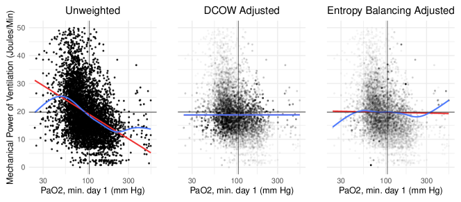
Figure 1: Shown are plots of the relationship between the minimum Pa$\text{O}_{2}$ on day 1 in the ICU (on a log base 10 scale) and the treatment, including an unadjusted plot (left) and plots adjusted by DCOWs and entropy balancing weights (right two plots). In the adjusted plots, the transparency of each point is proportional to its assigned weight, with lighter points indicating less weight. The blue line is a weighted nonparametric regression of the treatment on Pa$\text{O}_{2}$ (on the log base 10 scale) and the red line is a weighted linear regression.

For each method, we construct pointwise confidence bands of the ADRF using a nonparametric bootstrap similar to Wang and Wahba (1995). Weighted local linear regression estimates of the ADRF of mechanical power of ventilation on in-hospital mortality and 95% confidence bands are displayed in Figure 2. Alternatively, it is possible to conduct inference using the results of Theorem 3.7; however, doing so requires careful selection of the bandwidth parameter $h$, such as by using undersmoothing, which involves choosing a smaller bandwidth than the optimal one. Rigorous assessment of the use of Theorem 3.7 for inference is left as future work. The entropy balancing approach with higher order moments was not included due to the small effective sample size and a large number of bootstrap replications for which no solution was found. Both the entropy balancing weights and the GPS estimated with a normal model exhibit reasonable control over the dependence between covariates and treatment but result in unacceptably high variances in the estimate of the ADRF.

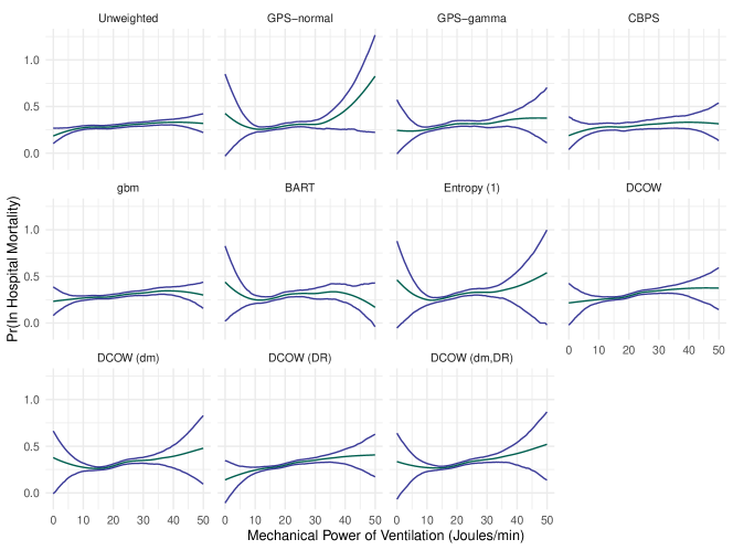
Figure 2: Shown are weighted local linear regression estimates of the ADRF of mechanical power on the probability of in-hospital mortality and pointwise 95% confidence bands estimated via a nonparametric bootstrap. 38 replications of the bootstrap resulted in no numerical solution for entropy balancing weights and are left out of the confidence interval calculation.

6 Discussion

In this paper, we provide a detailed inspection of the role of weights in weighted nonparametric estimates of causal quantities involving continuous-valued treatments from observational data. This inspection shows clearly that the key source of bias depends on the degree to which the weights induce independence between the treatment and confounders. We then provide a measure that characterizes how well a set of weights mitigates the dependence between the treatment and confounders. This measure does not require any tuning parameters, making it straightforward to deploy in practice. Given some light smoothness conditions on the outcome data-generating model, this measure acts as an upper bound on the key source of systematic bias in a weighted nonparametric estimate of the ADRF. Our proposed weights, the DCOWS, which minimize our measure of dependence, provide an empirically robust means for estimating weights, as they directly target independence between the treatment and confounders. These weights are a natural complement to doubly-robust estimators, as they provide an anchor for the doubly-robust estimator: since they are guaranteed to be consistent on their own, the consistency of the doubly-robust estimator does not critically depend on the correctness of the outcome model. Thus, the outcome model can be safely used as a tool to reduce variability in the estimate of the ADRF.

In contrast to other weighting approaches aimed at removing bias due to confounding with continuous treatments, the DCOWs enjoy a number of benefits that make them particularly attractive for applied use: they do not require any modeling of the relationship between the treatment or outcome and the covariates, they do not require the choice of specific features of the covariate distribution to balance, they do not require parameter tuning or cross-fitting, they perform well empirically (in addition to their strong asymptotic properties), and they can be readily implemented without specialized software using existing quadratic programming solvers. We have released an open-source implementation of our method in the R statistical computing language that can be used off-the-shelf to estimate the weights, available at https://github.com/jaredhuling/independenceWeights. Although our method, like all methods that adjust for confounding by measured confounders, requires that a sufficient set of confounding variables has been collected by the researcher, its ease of use helps alleviate the analytical burden of estimating the causal effects of continuous treatments in the presence of confounding by measured variables.

Appendix A Appendix: Regularity conditions

For $({\bf X}_{1},A_{1}),\dots,({\bf X}_{6},A_{6})\mathbin{\overset{i.i.d.}{\kern 0.0pt\sim}}F_{{\bf X},A}$, define the 6-th order kernel

$$k(({\bf X}_{1},A_{1}),\dots,({\bf X}_{6},A_{6}))=w^{*}({\bf X}_{1},A_{1})g_{\bf X}({\bf X}_{1},{\bf X}_{2},{\bf X}_{3},{\bf X}_{4})g_{A}(A_{1},A_{2},A_{5},A_{6})w^{*}({\bf X}_{2},A_{2})$$

with $w^{*}({\bf x},a)=\frac{f_{A}(a)}{f_{A|{\bf X}}(a|{\bf X}={\bf x})}$, $g_{\bf X}({\bf X}_{1},{\bf X}_{2},{\bf X}_{3},{\bf X}_{4})=\|{\bf X}_{1}-{\bf X}_{2}\|_{2}-\|{\bf X}_{1}-{\bf X}_{3}\|_{2}-\|{\bf X}_{2}-{\bf X}_{4}\|_{2}+\|{\bf X}_{3}-{\bf X}_{4}\|_{2}$, and $g_{A}(A_{1},A_{2},A_{3},A_{4})=|A_{1}-A_{2}|-|A_{1}-A_{3}|-|A_{2}-A_{4}|+|A_{3}-A_{4}|$. Further define the 4th order kernels

$$k_{\bf X}(({\bf X}_{1},A_{1}),\dots,({\bf X}_{4},A_{4}))={} w^{*}({\bf X}_{1},A_{1})\|{\bf X}_{1}-{\bf X}_{3}\|_{2}+w^{*}({\bf X}_{2},A_{2})\|{\bf X}_{2}-{\bf X}_{4}\|_{2}$$

$$-w^{*}({\bf X}_{1},A_{1})w^{*}({\bf X}_{2},A_{2})\|{\bf X}_{1}-{\bf X}_{2}\|_{2}-\|{\bf X}_{3}-{\bf X}_{4}\|_{2}\text{ and}$$

$$k_{A}(({\bf X}_{1},A_{1}),\dots,({\bf X}_{4},A_{4}))={} w^{*}({\bf X}_{1},A_{1})|A_{1}-A_{3}|+w^{*}({\bf X}_{2},A_{2})|A_{2}-A_{4}|$$

$$-w^{*}({\bf X}_{1},A_{1})w^{*}({\bf X}_{2},A_{2})|A_{1}-A_{2}|-|A_{3}-A_{4}|.$$

The following assumptions are required for several Lemmas and Theorems presented that rely on $V$-statistics. These conditions amount to finite moment conditions on squares of the Euclidean norms of ${\bf X}$, $A$ and their products with the weights $w^{*}({\bf X},A)$.

1. $\mathbb{E}[k^{2}(({\bf X}_{1},A_{1}),\dots,({\bf X}_{6},A_{6}))]<\infty$

2. $\mathbb{E}[k_{\bf X}^{2}(({\bf X}_{1},A_{1}),\dots,({\bf X}_{4},A_{4}))]<\infty$ and $\mathbb{E}[k_{A}^{2}(({\bf X}_{1},A_{1}),\dots,({\bf X}_{4},A_{4}))]<\infty$

Supplementary Material

Supplementary Material:

The Supplementary Material contains details for error decompositions of weighted nonparametric estimators, computational details of the proposed method, extended discussion of the existing literature, proofs of the theoretical results, and additional simulation studies. (pdf)

Acknowledgments

We would like to thank the Associate Editor and anonymous referees for their constructive feedback and suggestions Jue Hou for the helpful discussion. Chen’s effort was partially supported by NSF grant DMS-2054346 and the University of Wisconsin School of Medicine and Public Health from the Wisconsin Partnership Program.

References

- (1)
- Ai et al. (2021) Ai, C., Linton, O., Motegi, K. and Zhang, Z. (2021), ‘A unified framework for efficient estimation of general treatment models’, Quantitative Economics 12(3), 779–816.
- Chattopadhyay et al. (2020) Chattopadhyay, A., Hase, C. H. and Zubizarreta, J. R. (2020), ‘Balancing vs modeling approaches to weighting in practice’, Statistics in Medicine 39(24), 3227–3254.
- Colangelo and Lee (2020) Colangelo, K. and Lee, Y.-Y. (2020), ‘Double debiased machine learning nonparametric inference with continuous treatments’, arXiv preprint arXiv:2004.03036 .
- Crump et al. (2009) Crump, R. K., Hotz, V. J., Imbens, G. W. and Mitnik, O. A. (2009), ‘Dealing with limited overlap in estimation of average treatment effects’, Biometrika 96(1), 187–199.
- Díaz and van der Laan (2013) Díaz, I. and van der Laan, M. J. (2013), ‘Targeted data adaptive estimation of the causal dose–response curve’, Journal of Causal Inference 1(2), 171–192.
- Fan et al. (2021) Fan, J., Imai, K., Lee, I., Liu, H., Ning, Y. and Yang, X. (2021), ‘Optimal covariate balancing conditions in propensity score estimation’, Journal of Business & Economic Statistics pp. 1–14.
- Fong et al. (2018) Fong, C., Hazlett, C. and Imai, K. (2018), ‘Covariate balancing propensity score for a continuous treatment: Application to the efficacy of political advertisements’, The Annals of Applied Statistics 12(1), 156–177.
- Galvao and Wang (2015) Galvao, A. F. and Wang, L. (2015), ‘Uniformly semiparametric efficient estimation of treatment effects with a continuous treatment’, Journal of the American Statistical Association 110(512), 1528–1542.
- Hill (2011) Hill, J. L. (2011), ‘Bayesian nonparametric modeling for causal inference’, Journal of Computational and Graphical Statistics 20(1), 217–240.
- Hirano and Imbens (2004) Hirano, K. and Imbens, G. W. (2004), The Propensity Score with Continuous Treatments, John Wiley & Sons, Ltd, chapter 7, pp. 73–84.
- Huling and Mak (2020) Huling, J. D. and Mak, S. (2020), ‘Energy balancing of covariate distributions’, arXiv preprint arXiv:2004.13962 .
- Imai and Ratkovic (2014) Imai, K. and Ratkovic, M. (2014), ‘Covariate balancing propensity score’, Journal of the Royal Statistical Society: Series B (Statistical Methodology) 76(1), 243–263.
- Imai and Van Dyk (2004) Imai, K. and Van Dyk, D. A. (2004), ‘Causal inference with general treatment regimes: Generalizing the propensity score’, Journal of the American Statistical Association 99(467), 854–866.
- Imbens (2004) Imbens, G. W. (2004), ‘Nonparametric estimation of average treatment effects under exogeneity: A review’, Review of Economics and Statistics 86(1), 4–29.
- Johnson et al. (2016) Johnson, A. E., Pollard, T. J., Shen, L., Li-Wei, H. L., Feng, M., Ghassemi, M., Moody, B., Szolovits, P., Celi, L. A. and Mark, R. G. (2016), ‘Mimic-iii, a freely accessible critical care database’, Scientific data 3(1), 1–9.
- Johnson et al. (2003) Johnson, E., Dominici, F., Griswold, M. and L. Zeger, S. (2003), ‘Disease cases and their medical costs attributable to smoking: an analysis of the national medical expenditure survey’, Journal of Econometrics 112(1), 135–151.
- Kallus and Santacatterina (2019) Kallus, N. and Santacatterina, M. (2019), ‘Kernel optimal orthogonality weighting: A balancing approach to estimating effects of continuous treatments’, arXiv preprint arXiv:1910.11972 .
- Kang and Schafer (2007) Kang, J. D. and Schafer, J. L. (2007), ‘Demystifying double robustness: A comparison of alternative strategies for estimating a population mean from incomplete data’, Statistical Science 22(4), 523–539.
- Kennedy et al. (2017) Kennedy, E. H., Ma, Z., McHugh, M. D. and Small, D. S. (2017), ‘Non-parametric methods for doubly robust estimation of continuous treatment effects’, Journal of the Royal Statistical Society: Series B (Statistical Methodology) 79(4), 1229–1245.
- Kish (1965) Kish, L. (1965), Survey sampling, Vol. 26, John Wiley & Sons.
- Mak and Joseph (2018) Mak, S. and Joseph, V. R. (2018), ‘Support points’, The Annals of Statistics 46(6A), 2562–2592.
- Martinet (2020) Martinet, G. (2020), ‘A balancing weight framework for estimating the causal effect of general treatments’, arXiv preprint arXiv:2002.11276 .
- Naimi et al. (2014) Naimi, A. I., Moodie, E. E., Auger, N. and Kaufman, J. S. (2014), ‘Constructing inverse probability weights for continuous exposures: a comparison of methods’, Epidemiology pp. 292–299.
- Neto et al. (2018) Neto, A. S., Deliberato, R. O., Johnson, A. E., Bos, L. D., Amorim, P., Pereira, S. M., Cazati, D. C., Cordioli, R. L., Correa, T. D., Pollard, T. J. et al. (2018), ‘Mechanical power of ventilation is associated with mortality in critically ill patients: an analysis of patients in two observational cohorts’, Intensive Care Medicine 44(11), 1914–1922.
- Papazian et al. (2019) Papazian, L., Aubron, C., Brochard, L., Chiche, J.-D., Combes, A., Dreyfuss, D., Forel, J.-M., Guérin, C., Jaber, S., Mekontso-Dessap, A. et al. (2019), ‘Formal guidelines: management of acute respiratory distress syndrome’, Annals of Intensive Care 9(1), 1–18.
- Robins et al. (2000) Robins, J. M., Hernan, M. A. and Brumback, B. (2000), ‘Marginal structural models and causal inference in epidemiology’, Epidemiology 11, 550–560.
- Robins et al. (1994) Robins, J. M., Rotnitzky, A. and Zhao, L. P. (1994), ‘Estimation of regression coefficients when some regressors are not always observed’, Journal of the American Statistical Association 89(427), 846–866.
- Rosenbaum and Rubin (1983) Rosenbaum, P. R. and Rubin, D. B. (1983), ‘The central role of the propensity score in observational studies for causal effects’, Biometrika 70(1), 41–55.
- Sejdinovic et al. (2013) Sejdinovic, D., Sriperumbudur, B., Gretton, A. and Fukumizu, K. (2013), ‘Equivalence of distance-based and RKHS-based statistics in hypothesis testing’, The Annals of Statistics 41(5), 2263–2291.
- Stellato et al. (2020) Stellato, B., Banjac, G., Goulart, P., Bemporad, A. and Boyd, S. (2020), ‘Osqp: An operator splitting solver for quadratic programs’, Mathematical Programming Computation pp. 1–36.
- Székely and Rizzo (2013) Székely, G. J. and Rizzo, M. L. (2013), ‘Energy statistics: A class of statistics based on distances’, Journal of Statistical Planning and Inference 143(8), 1249–1272.
- Székely et al. (2007) Székely, G. J., Rizzo, M. L. and Bakirov, N. K. (2007), ‘Measuring and testing dependence by correlation of distances’, The Annals of Statistics 35(6), 2769–2794.
- Tübbicke (2022) Tübbicke, S. (2022), ‘Entropy balancing for continuous treatments’, Journal of Econometric Methods 11(1), 71–89.
- van der Laan and Robins (2003) van der Laan, M. J. and Robins, J. M. (2003), Unified methods for censored longitudinal data and causality, Springer Science & Business Media.
- Vegetabile et al. (2021) Vegetabile, B. G., Griffin, B. A., Coffman, D. L., Robbins, M. W., Cefalu, M. and McCaffrey, D. F. (2021), ‘Nonparametric estimation of population average dose-response curves using entropy balancing weights for continuous exposures’, Health Services and Outcomes Research Methodology 21(1), 69–110.
- Wang and Wahba (1995) Wang, Y. and Wahba, G. (1995), ‘Bootstrap confidence intervals for smoothing splines and their comparison to bayesian confidence intervals’, Journal of Statistical Computation and Simulation 51(2-4), 263–279.
- Wong and Chan (2017) Wong, R. K. and Chan, K. C. G. (2017), ‘Kernel-based covariate functional balancing for observational studies’, Biometrika 105(1), 199–213.
- Yiu and Su (2018) Yiu, S. and Su, L. (2018), ‘Covariate association eliminating weights: a unified weighting framework for causal effect estimation’, Biometrika 105(3), 709–722.
- Zhu et al. (2015) Zhu, Y., Coffman, D. L. and Ghosh, D. (2015), ‘A boosting algorithm for estimating generalized propensity scores with continuous treatments’, Journal of Causal Inference 3(1), 25–40.