Calculation of derivative of nucleon form factors in $N_{f}=2+1$ lattice QCD at $M_{\pi}=138$ MeV on a (5.5 fm)³ volume

Abstract

We present a direct calculation for the first derivative of the isovector nucleon form factors with respect to the momentum transfer $q^{2}$ using the lower moments of the nucleon 3-point function in the coordinate space. Our numerical simulations are performed using the $N_{f}=2+1$ nonperturbatively $O(a)$-improved Wilson quark action and Iwasaki gauge action near the physical point, corresponding to the pion mass $M_{\pi}=138$ MeV, on a (5.5 fm)⁴ lattice at a single lattice spacing of $a=0.085$ fm. In the momentum derivative approach, we can directly evaluate the mean square radii for the electric, magnetic, and axial-vector form factors, and also the magnetic moment without the $q^{2}$ extrapolation to the zero momentum point. These results are compared with the ones determined by the standard method, where the $q^{2}$ extrapolations of the corresponding form factors are carried out by fitting models. We find that the new results from the momentum derivative method are obtained with a larger statistical error than the standard method, but with a smaller systematic error associated with the data analysis. Within the total error range of the statistical and systematic errors combined, the two results are in good agreement. On the other hand, two variations of the momentum derivative of the induced pseudoscalar form factor at the zero momentum point show some discrepancy. It seems to be caused by a finite volume effect, since a similar trend is not observed on a large volume, but seen on a small volume in our pilot calculations at a heavier pion mass of $M_{\pi}=510$ MeV. Furthermore, we discuss an equivalence between the momentum derivative method and the similar approach with the point splitting vector current.

I Introduction

A discrepancy of experimental measurements of the proton charge radius, called the proton radius puzzle, has not been solved yet since the muonic hydrogen measurement was reported in 2010 Pohl et al. (2010). The values of the charge radius measured from both elastic electron-proton scattering and hydrogen spectroscopy agree with each other Mohr et al. (2016), while they differ from the one measured from the muonic hydrogen. Several experiments are carried out and also proposed to understand this discrepancy, see Ref. Karr et al. (2020) for a review of this puzzle. Lattice QCD calculation, which is a unique computational experiment to investigate the complicated strong interaction dynamics, based on the first principles of QCD, can tackle the problem as an alternative to actual experiments.

In lattice QCD calculation, the mean square (MS) charge radius can be determined from the slope of the electric nucleon form factor at $q^{2}=0$. Most calculations including our previous works Ishikawa et al. (2018); Shintani et al. (2019) and recent works Alexandrou et al. (2017a, b); Gupta et al. (2017); Capitani et al. (2019); Green et al. (2017); Alexandrou et al. (2019); Bali et al. (2020); Jang et al. (2020a, b); Alexandrou et al. (2021a); Djukanovic et al. (2021); Park et al. (2021); Alexandrou et al. (2021b) measure the form factor in $q^{2}\neq 0$ with discrete lattice momenta, and fit the data with appropriate functional forms, such as dipole form, in order to determine the form-factor slope at the zero momentum point. The choice of fit functions, however, gives rise to relatively large systematic error. Even in a fit using data set including at tiny $q^{2}$ data point, its systematic error still remains as large as the statistical error of 2% as presented in Ref. Shintani et al. (2019). Such systematic uncertainty needs to be reduced to draw any conclusion on a maximum discrepancy of about 4% observed in the three experiments.

Apart from the systematic error from the choice of fit functions we observed that there is a discrepancy of more than 10% between the experimental value and our result of the isovector root MS charge radius obtained from lattice QCD calculation at the physical point ($M_{\pi}=135$ MeV) on a (10.9 fm)³ volume Shintani et al. (2019). In our lattice QCD simulation, some systematic uncertainties stemming from the chiral extrapolation and finite volume effect are considered to be negligible. Furthermore, excited state contamination in the electric form factor is well controlled and not significant in our simulation, because strong dependence on the time separation between the source and sink operators was not observed. A possible source of this discrepancy could be the effect of finite lattice spacing though it seems too large for $O(a^{2})$ effect in our non-perturbative improved Wilson quark calculation. Our future calculations performed at the finer lattice spacing will reveal the presence of the systematic error due to the lattice discretization effect. Nevertheless, we are still pursuing other reasons. We are interested in recent development of another approach, called the momentum derivative method, which can directly calculate the slope of the form factor. In comparison to the standard approach, this method should be useful to pin down the source of the current discrepancy between our lattice result and the experimental value.

The momentum derivative method was proposed in Ref. Aglietti et al. (1994), where the slope is determined without assuming fit functions of the form factor. This method employs the moments of the 3-point function in the coordinate space, which can access the derivatives of the form factor with respect to the square of four-momentum transfer $q^{2}$ at vanishing $q^{2}$. This method and its variation were applied to the nucleon form factor with the vector current at the pion mass of $M_{\pi}=0.4$ GeV Bouchard et al. (2016), and the physical $M_{\pi}$ Alexandrou et al. (2020), respectively. Another method of the direct derivative calculation using the point splitting vector current was proposed in Ref. de Divitiis et al. (2012), and it was applied for the electric, magnetic, and axial-vector form factors at the physical $M_{\pi}$ in Ref. Hasan et al. (2018).

In this study we adopt the former method to calculate physical quantities, including the form-factor slopes determined at $q^{2}=0$ for both the vector and axial-vector channels, in (2+1)-flavor lattice QCD at very close to the physical $M_{\pi}$ on the (5.5 fm)³ spatial volume. The physical quantities obtained from the momentum derivative method are compared with those from the standard analysis for the form factors. Using similar simulation setup as described in our previous works Ishikawa et al. (2018); Shintani et al. (2019), possible systematic errors involved in the momentum derivative method are discussed by examining the effect of excited state contaminations with three source-sink separations and also by the finite volume study with two different volumes in our pilot calculations at a heavier pion mass of $M_{\pi}=0.51$ GeV. In this paper we also elucidate the equivalence between the above-mentioned two direct methods through the discussion of an infinitesimal transformation on the correlation functions. This study is regarded as a feasibility study towards more realistic calculation with the PACS10 configurations on the (10.9 fm)³ volume Shintani et al. (2019); Ishikawa et al. (2019a, b).

This paper is organized as follows. Section II explains definitions for the nucleon correlation functions and their derivative calculated by moments of the correlation functions used in this study. We also discuss the equality between two types of the direct methods, that were proposed in Ref. Aglietti et al. (1994) and Ref. Hasan et al. (2018), to calculate the derivative of the form factors in this section. The simulation parameters are described in Sec. III. The results from the derivative of nucleon correlation functions are presented in Sec. IV. Section V is devoted to summary of this study. In two appendices, we firstly describe how the momentum derivative method is associated with a partially quenched approximation and secondly summarize the results obtained from the standard analysis of the form factors.

All dimensionful quantities are expressed in units of the lattice spacing throughout this paper, unless otherwise explicitly specified. A bold-faced variable represents a three-dimensional vector.

II Calculation methods

II.1 Correlation function with momentum

The exponentially smeared quark operator $q_{S}(t,{\bf x})$ with the Coulomb gauge fixing is employed in this study to calculate the nucleon 2- and 3-point functions as

$$q_{S}(t,{\bf x})=\sum_{\bf y}\phi(|{\bf y}-{\bf x}|)q(t,{\bf y}),$$ (1)

where $q(t,{\bf x})$ presents a local quark operator, and the color and Dirac indexes are omitted. A smearing function $\phi(r)$ is given in a spatial extent of $L$ as

$$\phi(r)=\left\{\begin{array}[]{ll}1&(r=0)\\ Ae^{-Br}&(r<L/2)\\ 0&(r\geq L/2)\end{array}\right..$$ (2)

with two parameters $A$ and $B$. The nucleon 2-point function with the local sink operator is defined as

$$C_{LS}(t-t_{\rm src},{\bf x}-{\bf x}_{\rm src})=\frac{1}{4}{\rm Tr}\left[{\mathcal{P}}_{+}\langle 0|N_{L}(t,{\bf x})\overline{N}_{S}(t_{\rm src},{\bf x}_{\rm src})|0\rangle\right],$$ (3)

where ${\mathcal{P}}_{+}=(1+\gamma_{4})/2$, and the nucleon operator is given for the proton state by

$$N_{L}(t,{\bf x})=\epsilon_{abc}u^{T}_{a}(t,{\bf x})C\gamma_{5}d_{b}(t,{\bf x})u_{c}(t,{\bf x})$$ (4)

with $C=\gamma_{4}\gamma_{2}$, the up and down quark operators $u,d$, and $a,b,c$ being the color indexes. The smeared source operator $N_{S}(t,{\bf x})$ is the same as the local one $N_{L}(t,{\bf x})$, but all the quark operators $u,d$ are replaced by the smeared ones defined in Eq. (1). We also calculate the smeared sink 2-point function $C_{SS}(t,{\bf x})$, where $N_{L}(t,{\bf x})$ is replaced by $N_{S}(t,{\bf x})$. The momentum projected 2-point function is then given by

$$C_{XS}(t;{\bf p})=\sum_{\bf r}{e^{-i{\bf p}\cdot{\bf r}}}C_{XS}(t,{\bf r}),$$ (5)

with $X=L,S$ and a three-dimensional momentum ${\bf p}$. In a large $t$ region, the 2-point function behaves as a single exponential function,

$$C_{XS}(t;{\bf p})=\frac{E_{N}(p)+M_{N}}{2E_{N}(p)}Z_{X}(p)Z_{S}(p)e^{-tE_{N}(p)},$$ (6)

where $M_{N}$ and $E_{N}(p)$ are the nucleon mass and energy with the momentum $p\equiv|{\bf p}|$, respectively. The overlap of the nucleon operator to the nucleon state is defined by $\langle 0|N_{X}(0,{\bf 0})|N(p)\rangle=Z_{X}(p)u_{N}(p)$, where $u_{N}(p)$ is a nucleon spinor.

We evaluate the nucleon 3-point functions as

$$C^{k}_{{\mathcal{O}}_{\alpha}}(t-t_{\rm src},{\bf x}-{\bf x}_{\rm src})=\frac{1}{4}\sum_{\bf y}{\rm Tr}\left[{\mathcal{P}}_{k}\langle 0|N_{S}(t_{\rm sink},{\bf y})J^{\mathcal{O}}_{\alpha}(t,{\bf x})\overline{N}_{S}(t_{\rm src},{\bf x}_{\rm src})|0\rangle\right],$$ (7)

where ${\mathcal{P}}_{k}$ is a projection operator for ${\mathcal{P}}_{t}={\cal P}_{+}$ and ${\mathcal{P}}_{5j}={\mathcal{P}}_{+}\gamma_{5}\gamma_{j}$ for $j=x,y,z$, and $J^{\mathcal{O}}_{\alpha}$ is an isovector local current operator as $J^{\mathcal{O}}_{\alpha}=\overline{u}{\mathcal{O}}_{\alpha}u-\overline{d}{\mathcal{O}}_{\alpha}d$ with ${\mathcal{O}}_{\alpha}=\gamma_{\alpha},\gamma_{\alpha}\gamma_{5}$ for the vector ($V$) and axial-vector ($A$) currents, respectively.

The form factors in non-zero momentum transfers are calculated by the momentum projected 3-point function as

$$C^{k}_{{\mathcal{O}}_{\alpha}}(t;{\bf p})=\sum_{{\bf r}}e^{-i{\bf p}\cdot{\bf r}}C^{k}_{{\mathcal{O}}_{\alpha}}(t,{\bf r}).$$ (8)

We evaluate three types of 3-point function, $C^{t}_{V_{t}}(t;{\bf p})$, $C^{5j}_{V_{i}}(t;{\bf p})$, and $C^{5j}_{A_{i}}(t;{\bf p})$ for $i=x,y,z$ to obtain the electric and magnetic form factors, $G_{E}(q^{2}),G_{M}(q^{2})$, and the axial-vector and induced pseudoscalar form factors, $F_{A}(q^{2}),F_{P}(q^{2})$.

The asymptotic forms in $t\gg t_{\rm src}$ and $t_{\rm sink}\gg t$, where $t_{\rm src}$ and $t_{\rm sink}$ are defined in Eq. (7), for each 3-point function are given by

$$C^{t}_{V_{t}}(t;{\bf p}) = \frac{1}{Z_{V}}\widetilde{C}_{2}(t;{\bf p})e^{-M(t_{\rm sink}-t)}G_{E}(q^{2}),$$ (9)

$$C^{5j}_{V_{i}}(t;{\bf p}) = \frac{1}{Z_{V}}\widetilde{C}_{2}(t;{\bf p})e^{-M(t_{\rm sink}-t)}\frac{i\varepsilon_{ijk}q_{k}}{E_{N}(p)+M}G_{M}(q^{2}),$$ (10)

$$C^{5j}_{A_{i}}(t;{\bf p}) = \frac{1}{Z_{A}}\widetilde{C}_{2}(t;{\bf p})e^{-M(t_{\rm sink}-t)}\left[F_{A}(q^{2})\delta_{ij}-\frac{q_{i}q_{j}}{E_{N}(p)+M_{N}}F_{P}(q^{2})\right],$$ (11)

where the squared momentum transfer is given by $q^{2}=2M_{N}(E_{N}(p)-M_{N})$ with ${\bf q}={\bf p}$. The renormalization factors $Z_{V}$ and $Z_{A}$ are defined through the renormalization of the local vector and axial-vector currents on the lattice, respectively. All 3-point functions share a common part of $\widetilde{C}_{2}(t;{\bf p})$, which is similar to the asymptotic form of the 2-point function in Eq. (6),

$$\widetilde{C}_{2}(t;{\bf p})=\frac{E_{N}(p)+M_{N}}{2E_{N}(p)}Z_{S}(0)Z_{S}(p)e^{-tE_{N}(p)}.$$ (12)

However, $\widetilde{C}_{2}(t;{\bf p})$ is simply eliminated by considering the following ratio Gockeler et al. (2005); Hagler et al. (2003)

$${\cal R}^{k}_{{\cal O}_{\alpha}}(t;{\bm{p}})=\frac{C_{{\cal O}_{\alpha}}^{k}(t;{\bm{p}})}{C_{SS}(t_{\rm sink};{\bm{0}})}\sqrt{\frac{C_{LS}(t_{\rm sink}-t;{\bm{p}})C_{SS}(t;{\bm{0}})C_{LS}(t_{\rm sink};{\bm{0}})}{C_{LS}(t_{\rm sink}-t;{\bm{0}})C_{SS}(t;{\bm{p}})C_{LS}(t_{\rm sink};{\bm{p}})}},$$ (13)

which is constructed from a given 3-point function defined in Eqs. (9)–(11) with appropriate combination of 2-point functions (6). The ratios for each 3-point function give the following asymptotic values in the asymptotic region:

$${\cal R}^{t}_{V_{t}}(t;{\bm{p}}) = \frac{1}{Z_{V}}\sqrt{\frac{E_{N}(p)+M_{N}}{2E_{N}(p)}}G_{E}(q^{2}),$$ (14)

$${\cal R}^{5j}_{V_{i}}(t;{\bm{p}}) = \frac{1}{Z_{V}}\frac{i\varepsilon_{ijk}q_{k}}{\sqrt{2E_{N}(p)(E_{N}(p)+M_{N})}}G_{M}(q^{2}),$$ (15)

$${\cal R}^{5j}_{A_{i}}(t,{\bm{p}}) = \frac{1}{Z_{A}}\sqrt{\frac{E_{N}(p)+M_{N}}{2E_{N}(p)}}\left[F_{A}(q^{2})\delta_{ij}-\frac{q_{i}q_{j}}{E_{N}(p)+M_{N}}F_{P}(q^{2})\right],$$ (16)

which contain the respective form factors.

The MS radius of a form factor ${\cal G}_{O}(q^{2})$ is defined by

$$\langle r^{2}_{O}\rangle=\left.-\frac{6}{{\cal G}_{O}(0)}\frac{d{\cal G}_{O}(q^{2})}{dq^{2}}\right|_{q^{2}=0}$$ (17)

with ${\cal G}_{O}=G_{E},G_{M},F_{A}$. In the standard way to determine the MS radius, ${\cal G}_{O}(q^{2})$ is at first fitted by dipole, quadratic, and z-expansion forms Boyd et al. (1995); Hill and Paz (2010) given by

$${\cal G}_{O}(q^{2}) = \frac{{\cal G}_{O}^{d}(0)}{(1+c^{d}q^{2})^{2}}\ \ {\rm(dipole)},$$ (18)

$$= {\cal G}_{O}^{q}(0)+c_{1}^{q}q^{2}+c_{2}^{q}q^{4}\ \ {\rm(quadratic)},$$ (19)

$$= {\cal G}_{O}^{z}(0)+c_{1}^{z}z(q^{2})+c_{2}^{z}z(q^{2})^{2}+c_{3}^{z}z(q^{2})^{3}\ \ (\text{z-expansion}),$$ (20)

where the z-expansion makes use of a conformal mapping from $q^{2}$ to a new variable $z$ defined as

$$z(q^{2})=\frac{\sqrt{t_{\rm cut}+q^{2}}-\sqrt{t_{\rm cut}}}{\sqrt{t_{\rm cut}+q^{2}}+\sqrt{t_{\rm cut}}}$$ (21)

with $t_{\rm cut}=4M_{\pi}^{2}$ for $G_{E}$ and $G_{M}$, or with $t_{\rm cut}=9M_{\pi}^{2}$ for $F_{A}$, where $M_{\pi}$ corresponds to the simulated pion mass. Thanks to its rapid convergence of Taylor’s series expansion in terms of $z$, we employ a cubic z-expansion form as a model independent fit as described in our previous work Shintani et al. (2019). Using the resulting fit parameter given in each fit, the MS radius can be determined as

$$\langle r^{2}_{O}\rangle = \frac{12}{c^{d}}=-\frac{6}{{\cal G}_{O}^{q}(0)}c_{1}^{q}=-\frac{6}{{\cal G}_{O}^{z}(0)}\frac{c_{1}^{z}}{4t_{\rm cut}}.$$ (22)

II.2 Momentum derivatives of the 2- and 3-point functions

As proposed in Ref. Aglietti et al. (1994), the second-order momentum derivative of the 2-point function with respective to $p_{i}$ at the zero momentum point is calculated by

$$C_{LS}^{(2)}(t)=-\sum_{\bf r}r_{i}^{2}C_{LS}(t,{\bf r}),$$ (23)

where the summation is calculated over $-L/2+1\leq r_{i}\leq L/2$. The superscript (2) in $C_{LS}^{(2)}$ denotes the second-order derivative. In a large $t$ region, a ratio of the derivative function at the zero momentum point to the zero momentum 2-point function becomes

$$R_{2}(t)=\frac{C_{LS}^{(2)}(t)}{C_{LS}(t;{\bf 0})}=A+\frac{t}{M_{N}},$$ (24)

where the first term $A$ represents a constant contribution corresponding to the derivative of the amplitude in Eq. (6). It should be noted that the constant $A$ does not contain both the overlap with the local operator, $Z_{L}$, and its derivative. This is simply because $Z_{X}(p)$ becomes independent of $p$ for the local operator ($X=L$).

The derivative of the 3-point function with respective to the momentum is calculated in the same way as the one of the 2-point function in Eq. (23). We shall call the method to calculate the momentum derivatives of the 3-point functions as the derivative of form factor (DFF) method in the following. For the vector current, we construct the first, second and third-order derivatives of the 3-point function with the appropriate type of 3-point functions, $C^{t}_{V_{t}}(t,{\bf r})$ or $C^{5j}_{V_{i}}(t,{\bf r})$ as

$$C^{5j,(1)}_{V_{i},(k)}(t) = -i\sum_{\bf r}r_{k}C^{5j}_{V_{i}}(t,{\bf r}),$$ (25)

$$C^{t,(2)}_{V_{t},(l)}(t) = -\sum_{\bf r}r^{2}_{l}C^{t}_{V_{t}}(t,{\bf r}),$$ (26)

$$C^{5j,(3)}_{V_{i},(kl)}(t) = i\sum_{\bf r}r_{k}r^{2}_{l}C^{5j}_{V_{i}}(t,{\bf r}),$$ (27)

with $k\neq i\neq j$ and $l=x,y,z$. Respective ratios associated with the first to third-order derivatives are defined as

$$R_{V_{\alpha},(l)}^{k,(n)}(t)=\frac{C^{k,(n)}_{V_{\alpha},(l)}(t)}{C^{t}_{V_{t}}(t;{\bf 0})}.$$ (28)

with the vector three-point function with the zero momentum, $C^{t}_{V_{t}}(t;{\bf 0})$. The superscript $(n)$ denotes the $n$-th order derivative.

In this study, we will later determine the magnetic moment, MS charge radius, and MS magnetic radius from the ratios associated with the first-order derivative (25), second-order derivative (26) and third-order derivative (27), respectively, without the $q^{2}$ extrapolations of the corresponding form factors toward the zero momentum transfer.

For the axial-vector current, the following three types of the second-order derivatives are considered in the DFF method,

$$C^{5j,(2)}_{A_{j},(i)}(t) = -\sum_{\bf r}r_{i}^{2}C^{5j}_{A_{j}}(t,{\bf r}),$$ (29)

$$C^{5j,(2)}_{A_{j},(j)}(t) = -\sum_{\bf r}r_{j}^{2}C^{5j}_{A_{j}}(t,{\bf r}),$$ (30)

$$C^{5j,(2)}_{A_{i},(ij)}(t) = -\sum_{\bf r}r_{i}r_{j}C^{5j}_{A_{i}}(t,{\bf r}),$$ (31)

which are defined with $i\neq j$. Just as in the vector cases, the ratios associated with three types of the second-order derivatives are evaluated as below, to directly access the MS axial-vector radius and the value of $F_{P}(0)/g_{A}$ with the axial-vector coupling $g_{A}$,

$$R_{A_{\alpha},(l)}^{k,(2)}(t)=\frac{C^{k,(2)}_{A_{\alpha},(l)}(t)}{C^{5j}_{A_{j}}(t;{\bf 0})}$$ (32)

with $l=i,j,ij$.

In the asymptotic region of $t\gg t_{\rm src}$ and $t_{\rm sink}\gg t$, the ratios, which are associated with the $n$-th order derivatives defined in Eqs. (28) and (32), for $n\geq 2$, exhibit the following asymptotic behavior

$$R_{{\cal O}_{\alpha},(l)}^{k,(n)}(t)=C+A+\frac{t}{M_{N}},$$ (33)

where the first term $C$ represents a constant contribution that contains the MS radius of the form factor. The second and third terms can be identified with the contributions from the second-order derivative of $-\widetilde{C}_{2}(t;{\bf p})/\widetilde{C}_{2}(t;{\bf 0})$ in Eq. (12), whose values coincide with the ones evaluated from $R_{2}(t)$ defined in Eq. (24). Thus, the constant $C$ can be isolated using $R_{2}(t)$ to subtract the other two contributions from Eq. (33).

II.3 Equivalence on two definitions of momentum derivatives

In this subsection we intend to discuss an equivalence of the two direct derivative methods. In the following discussion, variables $x,y,z$ represent four-dimensional coordinates.

The momentum derivative of the quark propagator at the zero momentum is given by

$$\left.\frac{\partial G(x,y)e^{i{\bf p}\cdot({\bf x}-{\bf y})}}{\partial p_{j}}\right|_{{\bf p}=0}=-i(x_{j}-y_{j})G(x,y),$$ (34)

where $G(x,y)$ represents the quark propagator. This definition is employed in our calculation and Refs. Aglietti et al. (1994); Lellouch et al. (1995); Feng et al. (2020); Alexandrou et al. (2020). Another definition de Divitiis et al. (2012) of the momentum derivative is given by means of the point splitting vector current $\widetilde{\gamma}_{j}$ as

$$\left.\frac{\partial G_{p}(x,y)}{\partial p_{j}}\right|_{{\bf p}=0}=-i\sum_{z}G(x,z)\tilde{\gamma}_{j}(z)G(z,y),$$ (35)

where $G_{p}(x,y)$ represents the quark propagator calculated through the phase rotation of the gauge link as $U_{j}(x)\rightarrow e^{ip_{j}}U_{j}(x)$ with the phase associated with the momentum $p_{j}$. The definition of $\widetilde{\gamma}_{j}$ appearing in Eq.(35) is given by

$$f(x)\widetilde{\gamma}_{\mu}(x)g(x)=\frac{1}{2}\left[f(x+\hat{\mu})(1+\gamma_{\mu})U_{\mu}^{\dagger}(x)g(x)-f(x)(1-\gamma_{\mu})U_{\mu}(x)g(x+\hat{\mu})\right].$$ (36)

We will discuss an equivalence of the above two definitions as below.

Let us consider an infinitesimal transformation of the quark field $\psi(x)\to(1+i\alpha(x))\psi(x)$ with an arbitrary infinitesimal parameter $\alpha(x)$ depending on $x$. Requiring the invariance of the expectation value of the quark propagator under this transformation, one finds the following relation:

$$\delta(\langle\psi(x)\overline{\psi}(y)\rangle) = -i\sum_{z}(\partial^{f}_{\mu}\alpha(z))\langle\widetilde{V}_{\mu}(z)\psi(x)\overline{\psi}(y)\rangle+i(\alpha(x)-\alpha(y))\langle\psi(x)\overline{\psi}(y)\rangle=0,$$ (37)

where $\widetilde{V}_{\mu}(z)=\overline{\psi}(z)\widetilde{\gamma}_{\mu}(z)\psi(z)$ corresponds to the conserved vector current, and $\partial_{\mu}^{f}$ represents a forward difference. When $\alpha(x)=\varepsilon x_{j}$ with $\varepsilon\neq 0$, we obtain

$$-i\sum_{z}\langle\widetilde{V}_{j}(z)\psi(x)\overline{\psi}(y)\rangle=-i(x_{j}-y_{j})\langle\psi(x)\overline{\psi}(y)\rangle.$$ (38)

The right hand side of Eq. (38) coincides with the definition of the momentum derivative of the propagator used in our calculation, while the left hand side of Eq. (38) can be identified with the momentum derivative defined by Eq. (35). This discussion can be easily applied to hadronic correlators, and also extended to the higher-order derivatives by using the transformation repeatedly. The similar transformation can be applied to the temporal direction as well. Note that the left hand side of Eq. (38) receives contribution from the quark disconnected diagram in general, though it is absent if the isovector current is considered, or it can be neglected if a partially quenched approximation is applied. The former case will be explained below with the nucleon 2-point function, and the details of the latter case are described in Appendix A.

Here let us consider the proton 2-point function with the local operators having exact isospin symmetry. Performing the transformation of the $u$ quark fields in the 2-point function, one obtains the following relation

$$\langle 0|N_{L}(t,{\bf x})\sum_{z}\widetilde{V}^{u}_{\nu}(z)\overline{N}_{L}(0,{\bf 0})|0\rangle=2x_{\nu}\langle 0|N_{L}(t,{\bf x})\overline{N}_{L}(0,{\bf 0})|0\rangle,$$ (39)

where $\widetilde{V}^{u}_{\nu}$ is the conserved vector current for the $u$ quark. The factor of 2 comes from the fact that the proton operator has two $u$ quark fields. A similar relation is obtained through the same transformation of the $d$ quark fields as

$$\langle 0|N_{L}(t,{\bf x})\sum_{z}\widetilde{V}^{d}_{\nu}(z)\overline{N}_{L}(0,{\bf 0})|0\rangle=x_{\nu}\langle 0|N_{L}(t,{\bf x})\overline{N}_{L}(0,{\bf 0})|0\rangle,$$ (40)

where $\widetilde{V}^{d}_{\nu}$ is the conserved vector current for the $d$ quark. As for the isovector current $\widetilde{V}^{v}_{\nu}(z)=\overline{u}(z)\widetilde{\gamma}_{\nu}(z)u(z)-\overline{d}(z)\widetilde{\gamma}_{\nu}(z)d(z)$, the corresponding relation is given by a difference of the above two relations as,

$$\langle 0|N_{L}(t,{\bf x})\sum_{z}\widetilde{V}^{v}_{\nu}(z)\overline{N}_{L}(0,{\bf 0})|0\rangle=x_{\nu}\langle 0|N_{L}(t,{\bf x})\overline{N}_{L}(0,{\bf 0})|0\rangle,$$ (41)

where there is no contribution from quark disconnected diagrams in the left hand side, since they can be canceled due to exact isospin symmetry.

In our pilot calculations at a heavier pion mass of $M_{\pi}=0.51$ GeV, we verify the left and right equality of the above equation (41), i.e., the equivalence between the two definitions of the momentum derivative. We numerically confirm that they are reasonably consistent with each other through verification of the following two equations as,

$${\rm Tr}\left[{\mathcal{P}}_{+}\sum_{\bf x}\langle 0|N_{S}(t,{\bf x})\sum_{z}\widetilde{V}^{v}_{t}(z)\overline{N}_{S}(0,{\bf 0})|0\rangle\right] = t{\rm Tr}\left[{\mathcal{P}}_{+}\sum_{\bf x}\langle 0|N_{S}(t,{\bf x})\overline{N}_{S}(0,{\bf 0})|0\rangle\right],$$

$${\rm Tr}\left[{\mathcal{P}}_{+}\sum_{\bf x}x_{i}\langle 0|N_{L}(t,{\bf x})\sum_{z}\widetilde{V}^{v}_{i}(z)\overline{N}_{L}(0,{\bf 0})|0\rangle\right] = {\rm Tr}\left[{\mathcal{P}}_{+}\sum_{\bf x}x_{i}^{2}\langle 0|N_{L}(t,{\bf x})\overline{N}_{L}(0,{\bf 0})|0\rangle\right].$$

The numerical verification of Eq. (LABEL:eq:der_equiv1) is essentially the same as that of the renormalization factor of $Z_{\widetilde{V}}=1$. It should be noted that the equality described in Eq. (LABEL:eq:der_equiv2) is valid only if both the 2-point and 3-point functions are constructed by the local nucleon operators $N_{L}$. If the smeared nucleon operators $N_{S}$ are used, the corresponding relation becomes more complicated due to explicit spatial dependence of the smearing function, i.e., $\phi(r)$ appearing in Eq. (1). On the other hand, the equality described in Eq. (LABEL:eq:der_equiv1) can be applicable even for the smeared nucleon operators $N_{S}$, since the coordinate in the direction of the derivative is not spatial but temporal. The smearing function $\phi(r)$ is clearly independent of the temporal coordinate.

Finally, recall that the smeared nucleon source operator is adopted in our whole calculation. Thus, the quantity, which we actually calculated as defined in Eq. (23), may exhibit a slight difference from the right hand side of Eq. (LABEL:eq:der_equiv2) in the asymptotic region. This difference is absorbed only into the difference of the constant $A$, which is attributed to the difference in the overlaps to the nucleon, $Z_{X}(p)$, defined in Eq. (6), and also their derivatives, between $X=L$ and $S$. Therefore, it should not matter for extraction of the physical quantities using the DFF method.

Hereafter, we adopt the definition of Eq. (34) for the momentum derivative in our whole calculation, since the calculation cost of the right hand side in Eqs. (LABEL:eq:der_equiv1) and (LABEL:eq:der_equiv2) is much smaller than that of the left hand side.

III Calculation parameters

The configuration used in this study was generated with the Iwasaki gauge action Iwasaki (2011) and the six stout-smeared Clover quark action near the physical point for intended purpose where the finite-size study was done for light hadron spectroscopy in $N_{f}=2+1$ lattice QCD at the physical point Ishikawa et al. (2019a, b). The lattice size is $L^{3}\times T=64^{3}\times 64$ corresponding to (5.5 fm)⁴ with a lattice cutoff, $a^{-1}=2.3162(44)$ GeV Ishikawa et al. (2019b). Details of the parameters for the gauge configuration generation are summarized in Ref. Ishikawa et al. (2019a).

For the measurements for the nucleon correlation functions, the same quark action as in the gauge configuration generation is employed with the hopping parameter $\kappa=0.126117$ for the light quarks and the improved coefficient $c_{\rm SW}=1.11$ Taniguchi (2012). The quark propagator is calculated using the exponential smeared source in Eq. (1) with the Coulomb gauge fixing. The smearing parameters for the quark propagator are chosen as $(A,B)=(1.2,0.14)$ to obtain early plateau of the effective mass of $C_{LS}(t;{\bf 0})$ as shown in Fig. 1. The periodic boundary condition in all the temporal and spatial directions is adopted in the quark propagator calculation. The sequential source method is used to calculate the nucleon 3-point functions with $t_{\rm sep}=t_{\rm sink}-t_{\rm src}=12,14,$ and 16 corresponding to 1.02, 1.19, and 1.36 fm, respectively. Our main result is obtained with $t_{\rm sep}=14$, and the results of $t_{\rm sep}=12$ and 16 are used for comparison. These values of $t_{\rm sep}$ are the same as the ones used in our previous calculation Shintani et al. (2019), where significant excited state contributions were not observed in three particular form factors of $G_{E}$, $G_{M}$, and $F_{A}$.

The nucleon 2- and 3-point functions are measured with the 100 configurations separated by the 20 molecular dynamics trajectories. Their statistical errors are estimated by the jackknife method with the bin size of 80 trajectories. We use the all-mode-averaging (AMA) method Blum et al. (2013); Shintani et al. (2015); von Hippel et al. (2017) with the deflated Schwartz Alternative Procedure (SAP) Luscher (2004) and Generalized Conjugate Residual (GCR) Luscher (2007) for the measurements as in our previous work Shintani et al. (2019). We compute the combination of correlator with high-precision $O^{\rm org}$ and low-precision $O^{\rm approx}$ as

$$O^{\rm(AMA)}=\frac{1}{N_{\rm org}}\sum^{N_{\rm org}}_{f\in G}\big{(}O^{{\rm(org)}\,f}-O^{{\rm(approx)}\,f}\big{)}+\frac{1}{N_{G}}\sum^{N_{G}}_{g\in G}O^{{\rm(approx)}\,g},$$ (44)

where the superscript $f,\,g$ denotes the transformation under the lattice symmetry $G$. In our calculation, it is translational symmetry, e.g., changing the position of the source operator, and rotating the temporal direction using the hypercube symmetry of the configuration. $N_{\rm org}$ and $N_{G}$ are the numbers for $O^{\rm org}$ and $O^{\rm approx}$, respectively. The numbers and the stopping conditions of the quark propagator for the high and low-precision measurements are summarized in Table 1. We also take the average of the forward and backward 3-point functions, and also three 3-point functions with the projector ${\cal P}_{5j}$ in all the three spatial directions $j=x,y,z$ to increase statistics.

In our calculation we obtain $M_{\pi}=0.1382(11)$ GeV and $M_{N}=0.9499(27)$ GeV, which agree with the previous calculation done with the same configuration Ishikawa et al. (2019a, b). The result of $M_{N}$ is shown by the solid lines in Fig. 1, which is obtained from a single exponential fit of $C_{LS}(t;{\bf 0})$ in the asymptotic region. Although a little finite volume effect of 3 MeV was observed in the pion mass $M_{\pi}$ by comparing with results obtained on the $L=64$ and $L=128$ lattice volumes Ishikawa et al. (2019a), the finite volume effect was not seen in the nucleon mass $M_{N}$ Ishikawa et al. (2019b). For the renormalization factors, we adopt $Z_{V}=1/{\cal R}^{t}_{V_{t}}(t;{\bf 0})$ with $G_{E}(0)=1$, and $Z_{A}=0.9650(68)$ evaluated by the Schrödinger functional scheme Ishikawa et al. (2016). The physical quantities obtained from the DFF method are compared with the standard analysis of the form factors evaluated with the same configuration, and also the ones from the larger volume calculation of (10.9 fm)³ in Ref. Shintani et al. (2019). The parameters for the larger volume data used in the comparison are summarized in Table 2.

For a study of finite volume effect for physical quantities obtained from the DFF method, a small test calculation is carried out at a heavier pion mass of $M_{\pi}=0.51$ GeV using the $N_{f}=2+1$ configurations with $a^{-1}=2.194$ GeV generated in Ref. Yamazaki et al. (2012). The parameters for this study are tabulated in Table 3.

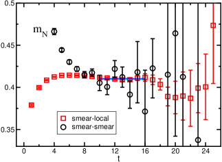
Figure 1: Effective mass for the nucleon from the smear-local (squared symbols) and smear-smear (circle symbols) cases of the nucleon 2-point functions, $C_{LS}(t;{\bf 0})$ and $C_{SS}(t;{\bf 0})$. Horizontal solid line represents a value of the nucleon mass obtained from $C_{LS}(t;{\bf 0})$ (smear-local) by a single exponential fit. Shaded band indicates its statistical error and the fitting range.

Table 1: Parameters for the AMA technique used in each choice of the source-sink separation ($t_{\rm sep}$): the stopping conditions of the quark propagator in the high- and low-precision measurements ($\epsilon_{\rm high}$ and $\epsilon_{\rm low}$), and the number of the measurements for the high- and low-precision calculations ($N_{\rm org}$ and $N_{G}$), respectively.

$t_{\rm sep}$	$\epsilon_{\rm high}$	$\epsilon_{\rm low}$	$N_{\rm org}$	$N_{G}$
12	$10^{-8}$	0.005	4	256
14	$10^{-8}$	0.005	4	1024
16	$10^{-8}$	0.002	4	2048

Table 2: Summary of simulation parameters used in this calculation together with those in the previous calculation performed on the larger volume Shintani et al. (2019): the spatial and temporal extents ($L$ and $T$), smearing parameters of the quark field ($A$ and $B$) defined in Eq. (1), separation of time slice between source and sink operators ($t_{\rm sep}$), the total number of the measurement ($N_{\rm meas}=N_{\rm conf}\times N_{G}$) given with the numbers for the configurations ($N_{\rm conf}$) and measurements per configuration ($N_{G}$), respectively. Recall that the previous results ($L=128$) are useful to be compared with the results obtained from the DFF method in this study.

$L$	$T$	$A$	$B$	$t_{\rm sep}$	$N_{\rm meas}$
64	64	1.2	0.16	12	25600
				14	102400
				16	204800
128	128	1.2	0.14	12	5120
				14	6400
				16	10218

Table 3: Details of parameters for the finite volume study at a heavier pion mass of $M_{\pi}=0.51$ GeV: the spatial and temporal extents ($L$ and $T$), separation of time slice between source and sink operators ($t_{\rm sep}$), smearing parameters of the quark field ($A$ and $B$) in Eq. (1), the numbers for the configurations ($N_{\rm conf}$) and measurements per configuration ($N_{G}$), respectively.

$L$	$T$	$t_{\rm sep}$	$A$	$B$	$N_{\rm conf}$	$N_{G}$
32	48	15	0.8	0.21	41	16
64	64	15	0.8	0.21	33	16

IV Results

In this section the results for the momentum derivatives of the nucleon 2- and 3-point functions are presented. Physical quantities obtained from the DFF method are compared with the ones from the standard analysis on the form factors. The results for the form factors given by the standard 3-point functions are summarized in Appendix B.

IV.1 Derivative of the nucleon 2-point function

Figure 2 presents the $t$ dependence of the ratio $R_{2}(t)$ defined in Eq. (24), where the second-order momentum derivative of the 2-point function (23) is divided by the the zero-momentum 2-point function. The dashed line represents a linear fit result given with the following form

$$R_{2}(t)=R_{2}^{0}+\frac{t}{M_{N}}$$ (45)

with a fit range of $t=10$–14, using the linear fixed slope with the measured $M_{N}$ obtained from the standard nucleon 2-point function. This fit result describes the data well in the large $t$ region, though in the small $t$ region we observe a deviation from the linear behavior which indicates the unwanted excited-state contributions appearing in the ratio. In the following analyses, the fit result $R_{2}^{0}$ is utilized to eliminate the common contribution in $R_{{\cal O}_{\alpha},(l)}^{k,(n)}(t)$ of Eq. (33) for $n\geq 2$, so as to extract the physical quantities of interest as discussed in Sec. II.2.

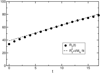
Figure 2: Ratio of the derivative of 2-point function to the standard 2-point function as a function of $t$. The statistical errors are comparable to the size of the symbols. The dashed line represents the linear fit of the large $t$ behavior on $R_{2}(t)$ as $R_{2}(t)=R_{2}^{0}+t/M_{N}$ with the measured $M_{N}$, where $R_{2}^{0}$ is only a free parameter.

IV.2 MS charge radius $\langle r_{E}^{2}\rangle$

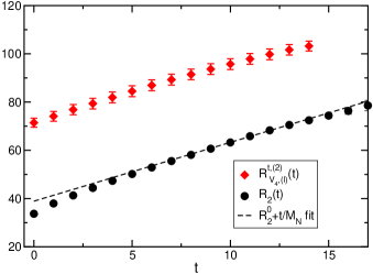
Figure 3: Ratio of the derivative of 3-point function to the standard zero-momentum 3-point function, $R_{V_{4},(l)}^{t,(2)}(t)$, for $G_{E}(q^{2})$ as a function of $t$ together with the corresponding one of 2-point function, $R_{2}(t)$, already shown in Fig. 2. A linear fit result of $R_{2}(t)$ is also plotted as the dashed line.

In the DFF method, the MS charge radius is extracted from $R_{V_{4},(l)}^{t,(2)}(t)$ with the second derivative of the 3-point function $C_{V_{4},(l)}^{t,(2)}(t)$, using its asymptotic form obtained with Eq. (26). The $t$ dependence of $R_{V_{4},(l)}^{t,(2)}(t)$ is presented in Fig. 3 together with the data of $R_{2}(t)$. The slope of $R_{V_{4},(l)}^{t,(2)}(t)$ reasonably agrees with the one of $R_{2}(t)$ as expected. At a glance, it is observed that $R_{V_{4},(l)}^{t,(2)}(t)$ has the smaller effect from excited states than the one appearing in $R_{2}(t)$, since the $t$ dependence of $R_{V_{4},(l)}^{t,(2)}(t)$ exhibits almost linear behavior even in a small $t$ region.

Considering the second derivative of $C^{t}_{V_{t}}(t;{\bf p})$, one finds the asymptotic form of $R_{V_{4},(l)}^{t,(2)}(t)$ as

$$R_{V_{4},(l)}^{t,(2)}(t)=\frac{\langle r_{E}^{2}\rangle}{3}+A+\frac{t}{M_{N}},$$ (46)

based on the asymptotic form of $C^{t}_{V_{t}}(t;{\bf p})$ given in Eq. (9), where we use the following relation

$$\left.\frac{\partial^{2}f(q^{2})}{\partial p_{l}^{2}}\right|_{{\bf p}=0}=2\frac{\partial f(0)}{\partial q^{2}}.$$ (47)

with $q^{2}=2M_{N}(E_{N}(p^{2})-M_{N})$ and the condition of ${\bf q}={\bf p}$.

As discussed in Sec II.2, the last two terms can be removed with $R_{2}(t)$ or a set of two quantities: $R_{2}^{0}$ obtained from $R_{2}(t)$ (through Eq. (45)) and the measured $M_{N}$ obtained from the standard spectroscopy.

Figure 4 shows the result of the effective MS charge radius $\langle r_{E}^{2}\rangle$ determined from

$$\langle r_{E}^{2}\rangle^{\rm eff}=3\left(R_{V_{4},(l)}^{t,(2)}(t)-R_{2}^{0}-\frac{t}{M_{N}}\right)$$ (48)

in each $t$ using two measured quantities of $R_{2}^{0}$ and $M_{N}$ (denoted as diamond symbols). For comparison, we also plot the result (denoted as circle symbols) given by a naive determination of $\langle r_{E}^{2}\rangle^{\rm eff}$ as $3(R_{V_{4},(l)}^{t,(2)}(t)-R_{2}(t))$ using the raw data of $R_{2}(t)$.

A little $t$ dependence is observed in the naive subtraction due to the non-negligible excited state contamination in $R_{2}(t)$ as explained earlier. Since the former value of $\langle r_{E}^{2}\rangle^{\rm eff}$ exhibits a flat region, we reliably determine $\langle r_{E}^{2}\rangle$ by a constant fit with the former value in the region of $t=5$–9 as drawn by the solid line together with the statistical error band. A systematic error is simply estimated by the maximum difference of the raw data in the fit region from the fit result. The combined error, where the statistical and systematic errors are added in quadrature, is shown in the figure by the dashed lines, although they are almost overlapped with the solid lines. The value of $\langle r_{E}^{2}\rangle$ obtained from the above analysis (denoted as the DFF method) is tabulated in Table 4. In the following analysis, the systematic error of quantities obtained from the DFF method will be quoted in the same manner as described above.

The result of $\langle r_{E}^{2}\rangle$ is compared with the one determined from the fitting of the $q^{2}$ dependence of $G_{E}(q^{2})$ in Fig. 4. The result of $\langle r_{E}^{2}\rangle$ obtained from the dipole fit defined in Eq. (18) on the data of $G_{E}(q^{2})$ has the smaller statistical error (inner error bar) than that of the above mentioned DFF method, while the rather large systematic uncertainty (outer error bar) on the fit result of $G_{E}(q^{2})$ is inevitable due to the choice of the fit form. A systematic error is estimated by maximum discrepancy of the results obtained with different fit forms, namely the quadratic and z-expansion forms as defined in Eqs. (19) and (20). Therefore, the results obtained from both the standard and DFF methods, are mutually consistent within the total errors whose sizes are comparable. The two results obtained in this study also reasonably agree with the previous result obtained from the standard method in our calculation performed on the larger volume ($L=128$) at the physical point Shintani et al. (2019).

It is worth mentioning that, compared to the values obtained from the standard calculation with the form factor $G_{E}(q^{2})$, the result of $\langle r_{E}^{2}\rangle$ in the DFF method is likely closer to both experimental values from the electron-proton scattering Mohr et al. (2016), 0.882(11) fm², and muonic hydrogen spectroscopy Antognini et al. (2013), 0.823(2) fm², while there remains a discrepancy of more than 10%. It might not be attributed to excited state contributions. The reason is that the data given with $t_{\rm sep}=12$ completely agrees with those with $t_{\rm sep}=14$ as shown in Fig. 5 in the DFF method. The data given with $t_{\rm sep}=16$ is also included in the figure, though it is too difficult to determine that there is an obvious dependency with respect to $t_{\rm sep}$ because of its large statistical errors. In Ref. Hasan et al. (2018), a large $t_{\rm sep}$ dependence was reported for the calculation of $\langle r_{E}^{2}\rangle$ using another derivative method. We, however, consider that it could be caused by their choice of smearing parameters for the quark operators, since our smearing parameters are highly optimized to eliminate the excited state contributions in the nucleon 2-point and 3-point functions.

The finite volume effect is other possible source of the systematic errors in the DFF method. The large effect on the quantity of $\langle r_{E}^{2}\rangle$ is not observed in our standard analyses with the form factor $G_{E}(q^{2})$ obtained from the $L=64$ and $L=128$ lattice data shown in Appendix B. A significant effect, however, is reported in a previous study in momentum derivative calculations of meson correlation functions Lellouch et al. (1995), and also found in our pilot study of $\langle r_{E}^{2}\rangle^{\rm eff}$ at a heavier pion mass of $M_{\pi}=0.51$ GeV. Figure 6 shows that there is a large discrepancy of $\langle r_{E}^{2}\rangle^{\rm eff}$ on volumes of the spacial extent of 2.9 and 5.8 fm at $M_{\pi}=0.51$ GeV, while the two results determined from the form factor in the standard way are highly consistent with each other and also the larger volume result from the DFF method.

Thus, for a precise determination of $\langle r_{E}^{2}\rangle$, it is an important future task to investigate the systematic uncertainty in the DFF method due to the finite size effect near the physical point, using our large volume configuration of $L=128$. Finally, we remark on an attempt of the improved analysis in the DDF method for the case of meson form factors Lellouch et al. (1995); Feng et al. (2020) in order to reduce the finite volume effect. This improvement can be also extended to the nucleon form factors.

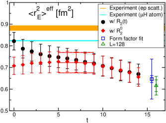
Figure 4: Effective MS charge radius $\langle r_{E}^{2}\rangle^{\rm eff}$ as a function of $t$, determined from $R_{V_{4},(l)}^{t,(2)}(t)$ with the data of $R_{2}(t)$ (circle symbols) and the values of $R_{2}^{0}$ and $M_{N}$ (diamond symbols), respectively. The solid red line represents a constant fit result on the diamond symbols, and its statistical error. The dashed lines appearing slightly outside the solid lines represent the total error. The MS radius determined from the standard analysis of $G_{E}(q^{2})$ in this calculation on the $L=64$ lattice volume is plotted by the square symbol, and the one obtained on the $L=128$ lattice volume Shintani et al. (2019) is also included by the triangle symbol. The inner and outer errors of these results represent the statistical and total errors, respectively. Here, the total errors are evaluated by adding the statistical and systematic errors in quadrature. The two horizontal bands represent experimental results from $ep$ scattering (upper) Mohr et al. (2016) and $\mu$-H atom spectroscopy (lower) Antognini et al. (2013).

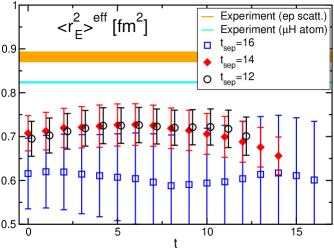
Figure 5: Comparison of the effective MS charge radius $\langle r_{E}^{2}\rangle^{\rm eff}$ obtained with $t_{\rm sep}=12$ (circle symbols), 14 (diamond symbols), and 16 (square symbols), respectively. The data of $t_{\rm sep}=12$ are slightly shifted to the positive $x$ direction for clarity. The two horizontal bands represent experimental results from $ep$ scattering (upper) Mohr et al. (2016) and $\mu$-H atom spectroscopy (lower) Antognini et al. (2013).

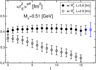
Figure 6: Finite volume study of $\langle r_{E}^{2}\rangle^{\rm eff}$ at a heavier pion mass of $M_{\pi}=0.51$ GeV. Filled and open circle symbols represent the data of the spatial extent of 5.8 fm and 2.9 fm, respectively. The square symbols correspond to the dipole fit results of the form factor $G_{E}(q^{2})$ on the larger (filled symbols) and smaller (open symbols) spatial volume.

Table 4: Summary of physical quantities obtained from the DFF method and also the corresponding ones evaluated in the standard analysis with the respective form factors. The raw data of the form factors are summarized in Appendix B. For comparison, the larger volume ($L=128$) results, which are given by the average of results from $t_{\rm sep}=12$, 14 and 16 within the standard analysis in our previous calculation Shintani et al. (2019), are also tabulated.

	$\langle r_{E}^{2}\rangle$ [fm2]	$\mu$	$\langle r_{M}^{2}\rangle$ [fm2]	$\langle r_{A}^{2}\rangle$ [fm2]
DFF method	0.722(47)(8)	4.337(73)(31)	0.397(46)(24)	0.341(35)(13)
form factor($L=64$)	0.646(16)(91)	4.36(4)(82)	0.58(2)(2.67)	0.308(17)(52)
form factor($L=128$)	0.616(27)(33)	4.41(14)(33)	0.500(51)(440)	0.283(30)(77)

IV.3 Magnetic moment $\mu$

The magnetic moment $\mu=G_{M}(0)$ in the DFF method is calculated from $R^{5j,(1)}_{V_{i},(k)}(t)$ with the first derivative of the 3-point function $C^{5j,(1)}_{V_{i},(k)}(t)$, using its asymptotic form obtained with Eq. (25). The effective magnetic moment is defined by

$$\mu^{\rm eff}=2M_{N}R^{5j,(1)}_{V_{i},(k)}(t)$$ (49)

with $k\neq i\neq j$, whose form can be read off by considering the derivative of the asymptotic form of $C^{5j}_{V_{i}}(t;{\bf p})$ in Eq. (10). It is here worth pointing out that the ratio $R^{5j,(1)}_{V_{i},(k)}(t)$ is supposed to show no dependence of $t$ in the asymptotic region.

Figure 7 presents that the data of $\mu^{\rm eff}$ exhibits a long flat region. The value of $\mu$ is again determined from a constant fit of the data in the region of $t=5$–9. The fit result of $\mu$ (denoted as the DFF method) is tabulated in Table 4. As a result, the total error of the DFF result is dominated only by the statistical error as same in the case of $\langle r_{E}^{2}\rangle^{\rm eff}$. As shown in Fig. 7, a reasonable consistency between $\mu$ obtained by the DFF method and the dipole fit result of $G_{M}(q^{2})$ is observed. However, the fit result of $G_{M}(q^{2})$ receives the large systematic uncertainty due to the choice of the fit form. Indeed, it is mainly caused by the z-expansion fit result of $G_{M}(q^{2})$, where unnatural vending down behavior towards $q^{2}=0$ is observed in the data of the $L=64$ lattice volume. It was less likely to happen in our previous study with the larger volume ($L=128$), where the lowest $q^{2}$ becomes closer to $q^{2}=0$.

Recall that for the case of $G_{M}(q^{2})$, $G_{M}(0)$ cannot be directly measured in the standard method for kinematical reasons. Therefore, the determination by the fitting of the $q^{2}$ dependence of $G_{M}(q^{2})$ is sometimes suffered from the large model dependence of the fit form because of the absence of the $G_{M}(0)$ data. For this reason, the systematic error on the DFF result in the smaller volume calculation is in general much better controlled than that of the fit result obtained even from the larger volume calculation.

The result in the DFF method is in good agreement with the two fit results of $G_{M}(q^{2})$ obtained in this study ($L=64$) and also from the larger volume calculation ($L=128$) Shintani et al. (2019). However, the significant reduction of the systematic error in the DFF method may expose an underestimation of $\mu$ in comparison with the experimental value, $\mu=4.70589$, in PDG20 Zyla et al. (2020). In order to investigate possible other systematic errors in the DFF method, the direct comparison of the data with $t_{\rm sep}=12$, 14, and 16 is first presented in Fig. 8. The three data statistically agree with each other in the middle $t$ region. We thus consider that the present data set shows no significant uncertainty associated with the excited state contamination in the data of $t_{\rm sep}=14$, though the statistical error of $t_{\rm sep}=16$ is larger than those for the other two data.

We rather consider that the discrepancy from the experiment might be caused again by a finite volume effect. As shown in Fig. 9, in our pilot study of the DFF method at $M_{\pi}=0.51$ GeV, we observe a large finite volume effect of more than 10% in comparison with the data on the (2.9 fm)³ and (5.8 fm)³ volumes even far away from the physical point. Note that the two dipole-fit results obtained with two spatial extents of $L=64$ and $L=128$ at the physical point agree with each other within the standard method, and thus such a large effect is not detected in the standard form factor calculation. More detailed investigations are required for full control of possible systematic errors in the DFF method in order to resolve the discrepancy mentioned above.

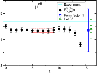
Figure 7: Same as Fig. 4 for the effective magnetic moment $\mu^{\rm eff}$ defined in Eq. (49). The cyan band represents the experimental result Zyla et al. (2020).

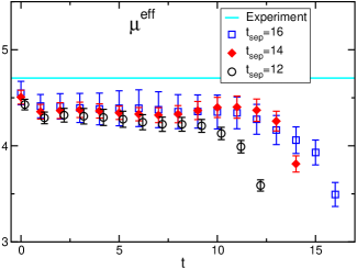
Figure 8: Same as Fig. 5 for the effective magnetic moment $\mu^{\rm eff}$. The cyan band represents the experimental result Zyla et al. (2020).

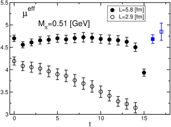
Figure 9: Same as Fig. 6 for the effective magnetic moment $\mu^{\rm eff}$.

IV.4 MS magnetic radius $\langle r_{M}^{2}\rangle$

Considering the third derivative of $C^{5j}_{V_{i}}(t;{\bf p})$ and its asymptotic form obtained with Eq. (10), $R^{5j,(3)}_{V_{i},(kl)}(t)$ yields the following asymptotic form:

$$R^{5j,(3)}_{V_{i},(kl)}(t)=\frac{\mu}{2M_{N}}\left(\frac{\langle r_{M}^{2}\rangle}{3}+\frac{1}{2M_{N}^{2}}+A+\frac{t}{M_{N}}\right),$$ (50)

with $l\neq k$ where $l$ and $k$ are the directions of the derivative defined in Eq. (27). When $l=k$ is set in Eq. (27), the right hand side of the above equation is multiplied by a factor of three. In our analysis all the $l$ data are averaged.

Using the asymptotic form of Eq. (50), the effective MS magnetic radius in the DFF method is determined by

$$\langle r_{M}^{2}\rangle^{\rm eff}=3\left(\frac{R^{5j,(3)}_{V_{i},(kl)}(t)}{R^{5j,(1)}_{V_{i},(k)}(t)}-\frac{1}{2M_{N}^{2}}-R_{2}^{0}-\frac{t}{M_{N}}\right)$$ (51)

with the first derivative $R^{5j,(1)}_{V_{i},(k)}(t)$ described in the previous subsection. The data of $\langle r_{M}^{2}\rangle^{\rm eff}$ plotted in Fig. 10 exhibits the milder $t$ dependence in small $t$ region compared to the data from a naive subtraction with the raw data of $R_{2}(t)$, $3({R^{5j,(3)}_{V_{i},(kl)}(t)}/{R^{5j,(1)}_{V_{i},(k)}(t)}-{1}/{(2M_{N}^{2})}-R_{2}(t))$ for the same reason as in the case of $\langle r_{E}^{2}\rangle^{\rm eff}$. In the middle $t$ region the two results are mutually consistent, so that we determine the value of $\langle r_{M}^{2}\rangle$ by a constant fit of $\langle r_{M}^{2}\rangle^{\rm eff}$ in the region of $t=5$–9, which is plotted by the solid lines in Fig. 10, and tabulated in Table 4. Although the statistical error of $\langle r_{M}^{2}\rangle$ obtained from the fit of $G_{M}(q^{2})$ on the $L=64$ lattice volume is smaller than that of the DFF method, much larger systematic error regarding the choice of fit function makes their total accuracy worse than the DFF result.

While the result of $\langle r_{M}^{2}\rangle$ given in the DFF method has smaller systematic error, its central value is much smaller than the experimental value, $\langle r_{M}^{2}\rangle=0.733(32)$ fm² Zyla et al. (2020). It might be caused by a finite volume effect in the DFF calculation, since this quantity is indeed considered to be more sensitive to finite volume effects compared to other quantities discussed earlier. In the DFF method, the quantity of $\langle r_{M}^{2}\rangle$ requires the third derivative of the 3-point function i.e., the third moment of the 3-point function in coordinate space. Therefore, the larger spatial extent is naturally required for its higher moment compared to the other quantities considered in the previous subsections. Figure 11 shows that in our pilot calculation of $\langle r_{M}^{2}\rangle^{\rm eff}$ at $M_{\pi}=0.51$ GeV, more significant finite volume effect is observed than the case of $\langle r_{E}^{2}\rangle^{\rm eff}$ in Fig. 6: the data of $\langle r_{M}^{2}\rangle^{\rm eff}$ on the smaller volume becomes negative in a large $t$ region in contrast to that of $\langle r_{E}^{2}\rangle^{\rm eff}$.

Another possible source of systematic errors comes from the excited state contamination. Comparing the three data sets using $t_{\rm sep}=12,$ 14, and 16 in Fig. 12, the $t_{\rm sep}$ dependence is not clearly seen due to their large statistical fluctuations. In a future work, it is important to investigate the above two systematic errors by calculations with the larger volume ($L=128$) and the large variation of $t_{\rm sep}$.

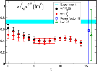
Figure 10: Same as Fig. 4 for the effective MS magnetic radius $\langle r_{M}^{2}\rangle^{\rm eff}$ obtained from $R^{5j,(3)}_{V_{i},(kl)}(t)$. The cyan band represents the experimental result Zyla et al. (2020).

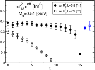
Figure 11: Same as Fig. 6 for the effective MS magnetic radius $\langle r_{M}^{2}\rangle^{\rm eff}$.

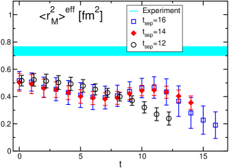
Figure 12: Same as Fig. 5 for the effective MS magnetic radius $\langle r_{M}^{2}\rangle^{\rm eff}$. The cyan band represents the experimental result Zyla et al. (2020).

IV.5 MS axial radius $\langle r_{A}^{2}\rangle$

For the MS axial radius $\langle r_{A}^{2}\rangle$, the same analysis as in the case of $\langle r_{E}^{2}\rangle$ with $R_{V_{4},(l)}^{t,(2)}(t)$ is performed for $R_{A_{j},(i)}^{5j,(2)}(t)$, where $i\neq j$ in the subscript expresses the direction of the derivative defined in Eq. (29). The asymptotic form of $R_{A_{j},(i)}^{5j,(2)}(t)$ is given by

$$R_{A_{j},(i)}^{5j,(2)}(t)=\frac{\langle r_{A}^{2}\rangle}{3}+A+\frac{t}{M_{N}}.$$ (52)

The effective MS axial-vector radius is defined by

$$\langle r_{A}^{2}\rangle^{\rm eff}=3\left(R_{A_{j},(i)}^{5j,(2)}(t)-R_{2}^{0}-\frac{t}{M_{N}}\right),$$ (53)

and its value is plotted as a function of $t$ in Fig. 13. The data is compared with the one determined from a naive subtraction with the raw data of $R_{2}(t)$ as $3(R_{A_{j},(i)}^{5j,(2)}(t)-R_{2}(t))$. Both estimations for $\langle r_{A}^{2}\rangle^{\rm eff}$ exhibit a reasonably flat behavior in the middle $t$ region, respectively. We determine the value of $\langle r_{A}^{2}\rangle$ by a constant fit of the data of $\langle r_{A}^{2}\rangle^{\rm eff}$ in the region of $t=5$–9. The result obtained by the DFF method is tabulated in Table 4. As shown in Fig. 13, the DFF result is fairly consistent with the two dipole-fit results of $F_{A}(q^{2})$ obtained in this study ($L=64$) and also from the larger volume calculation ($L=128$) Shintani et al. (2019). Again, the total accuracy of the dipole fit results is slightly worse than the DFF result that can avoid any model dependence.

As in the case of the dipole fit results, the result of the DFF method is little smaller than the experiment Bernard et al. (2002); Bodek et al. (2008), 0.449(13) fm². It can be attributed to excited state contamination. It is simply because a visible difference between the data from $t_{\rm sep}=12$ and 14 is seen in the flat region of $\langle r_{A}^{2}\rangle^{\rm eff}$ as a function of $t$ as shown in Fig. 14. Furthermore, the data of $t_{\rm sep}=16$ statistically agrees with the experiment, though the statistical uncertainties are not small enough to make a firm conclusion. In addition, recently, it was reported that a large effect due to the excited state contamination exists in determination of $\langle r_{A}^{2}\rangle$ even from the fitting of the $q^{2}$ dependence of $F_{A}(q^{2})$ Jang et al. (2020a); Park et al. (2021). Since we have only a few variations of $t_{\rm sep}$, we will need to verify whether or not the discrepancy from the experiment can be explained by the systematic uncertainties from the excited state contamination using the data with the larger variation of $t_{\rm sep}$. It is worth pointing out that the systematic error associated with the finite volume effect in $\langle r_{A}^{2}\rangle^{\rm eff}$ might be smaller than the other quantities obtained from the DFF method discussed earlier. This is expected from our pilot calculation at $M_{\pi}=0.51$ GeV as shown in Fig. 15. The difference between the data on the larger and smaller volumes is about 10% in the middle $t$ region, which it is much smaller than those of other quantities as shown in Figs. 6, 9, and 11.

The size of the finite volume effect is supposed to depend on the MS radius of the target form factor. If the MS radius is small, in other words, the form factor has a broad shape in the $q^{2}$ space, its moment in the coordinate space is less sensitive to the finite volume. This is because the narrow spatial distribution in the coordinate space is given by the inverse Fourier transform of the broad form factor in a classical argument. 

Indeed, the three values of $\langle r_{A}^{2}\rangle$ at $M_{\pi}=0.51$ GeV, which are obtained from the DFF method on the larger volume ($L=64$) and the dipole fit results obtained from both two volumes ($L=32$ and $L=64$) as shown in Fig. 15, are certainly smaller than those for $\langle r_{E}^{2}\rangle$ and $\langle r_{M}^{2}\rangle$. This observation leads to the expectation that $\langle r_{A}^{2}\rangle^{\rm eff}$ has the smaller finite volume effect. This expectation should remain valid at the physical $M_{\pi}$, since the experimental value of $\langle r_{A}^{2}\rangle$ is smaller than those of $\langle r_{E}^{2}\rangle$ and $\langle r_{M}^{2}\rangle$.

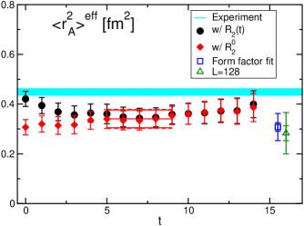
Figure 13: Same as Fig. 4 for the effective MS axial-vector radius $\langle r_{A}^{2}\rangle^{\rm eff}$ obtained from $R_{A_{j},(i)}^{5j,(2)}(t)$. The cyan band represents the experimental result Bernard et al. (2002); Bodek et al. (2008).

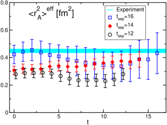
Figure 14: Same as Fig. 5 for the effective MS axial-vector radius $\langle r_{A}^{2}\rangle^{\rm eff}$. The cyan band represents the experimental result Bernard et al. (2002); Bodek et al. (2008).

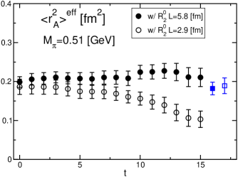
Figure 15: Same as Fig. 6 for the effective MS axial-vector radius $\langle r_{A}^{2}\rangle^{\rm eff}$.

IV.6 $F_{P}(0)$ from the DFF method

As same in the case of $G_{M}(0)$, $F_{P}(0)$ cannot be directly measured in the standard method for kinematical reasons. In the DFF method, the value of $F_{P}(0)$ is accessible in two ways. One uses $R_{A_{i},(ij)}^{5j,(2)}(t)$ with $i\neq j$ as defined in Eq. (30), while the other uses $R_{A_{j},(j)}^{5j,(2)}(t)$ defined in Eq. (31). Their asymptotic forms are given by

$$R_{A_{i},(ij)}^{5j,(2)}(t) = \frac{F_{P}(0)}{2M_{N}g_{A}},$$ (54)

$$R_{A_{j},(j)}^{5j,(2)}(t) = \frac{\langle r_{A}^{2}\rangle}{3}+A+\frac{t}{M_{N}}+\frac{F_{P}(0)}{M_{N}g_{A}},$$ (55)

where $i\neq j$. Using them, the effective value of $2M_{N}F_{P}(0)/g_{A}$ can be defined in two ways as

$$\frac{2M_{N}F_{P}^{\rm eff}(0)}{g_{A}} = 4M_{N}^{2}R_{A_{i},(ij)}^{5j,(2)}(t)$$ (56)

$$= 2M_{N}^{2}\left(R_{A_{j},(j)}^{5j,(2)}(t)-R_{A_{j},(i)}^{5j,(2)}(t)\right),$$ (57)

where the second term of $R_{A_{j},(i)}^{5j,(2)}$ appearing in Eq. (57) is the one used for the determination of $\langle r_{A}^{2}\rangle^{\rm eff}$ as discussed in the last subsection.

Figure 16 shows that the two different estimations of $2M_{N}F_{P}^{\rm eff}(0)/g_{A}$ with $t_{\rm sep}=14$ (denoted with filled symbols) provide inconsistent results: the result obtained from Eq. (56) is much smaller than that of Eq. (57). The same behavior is also seen in the data from the smaller and larger source-sink separations for $t_{\rm sep}=12$ and 16. Note that the expected value of $2M_{N}F_{P}(0)/g_{A}$ is much larger than these two observed values according to the following reasons: (1) $2M_{N}F_{P}(q^{2}_{1})/g_{A}\sim 40$ is observed even at the lowest non-zero $q^{2}=q_{1}^{2}$ in the standard method with $t_{\rm sep}=14$. (2) The $q^{2}$ dependence of $F_{P}(q^{2})$ is expected to rapidly increase in the limit of $q^{2}\to 0$ as shown in Appendix B.

This difference between the two estimations of $2M_{N}F_{P}^{\rm eff}(0)/g_{A}$ can be attributed to a finite volume effect. This is simply because a similar trend is observed in our pilot calculation at $M_{\pi}=0.51$ GeV, where the discrepancy between the two results becomes resolved in a larger volume calculation as shown in Fig. 17. A large systematic effect stemming from the finite volume is easily understood in this case, since the induced pseudoscalar form factor in the coordinate space, which corresponds to the one given by the inverse Fourier transform of $F_{P}(q^{2})$, has a very broad structure. This is naively expected from the fact that $F_{P}(q^{2})$ has a sharp peak near the origin at the physical $M_{\pi}$ corresponding to the large contribution of the pion pole in the pion pole dominance model. The moment of such a broad function in the coordinate space could not avoid the strong dependence of the finite volume.

In addition to the finite volume effect, in our previous studies, we observed other problem that the lattice data of $F_{P}(q^{2})$ differs from the pion pole dominance model Sasaki and Yamazaki (2008); Ishikawa et al. (2018), which can be explained by large excited state contamination Shintani et al. (2019). Similar discussions were reported in Refs. Bar (2019); Jang et al. (2020a); Alexandrou et al. (2021a); Jang et al. (2020b); Park et al. (2021). In order to fully resolve the problems, more comprehensive investigations are necessary in this particular quantity.

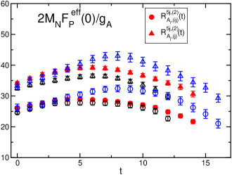
Figure 16: Effective induced pseudoscalar coupling $2M_{N}F_{P}(0)/g_{A}$ evaluated from $R_{A_{i},(ij)}^{5j,(2)}(t)$ (circle symbols) and $R_{A_{j},(j)}^{5j,(2)}(t)$ (triangle symbols). The black, red and blue symbols represent the data obtained with $t_{\rm sep}=12,14$ and 16.

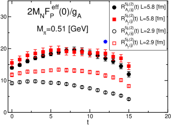
Figure 17: Finite volume study of effective induced pseudoscalar coupling $2M_{N}F_{P}(0)/g_{A}$ at a heavier pion mass of $M_{\pi}=0.51$ GeV. Filled and open circle symbols represent the data of the spatial extent of 5.8 fm and 2.9 fm, respectively. Circle and square symbols are determined with the definitions given in Eqs. (56) and (57), respectively. The single diamond symbol represents the value of $2M_{N}F_{P}(0)/g_{A}$ evaluated by examining the $q^{2}$ dependence of the form factor $F_{P}(q^{2})$ on the larger volume ($L=128$).

V Summary

We have calculated the MS radii and magnetic moment for the isovector nucleon form factors using the DFF method, which is a direct calculation method of the derivative of the form factor proposed in Ref. Aglietti et al. (1994), in the $N_{f}=2+1$ QCD near the physical point on the (5.5 fm)³ volume. We have also discussed an equivalence of the method used in this study to another derivative method de Divitiis et al. (2012).

The results from the DFF method near the physical point are compared with the ones from the standard form factor calculation on the same volume ($L=64$) and also on the larger volume ($L=128$) in our previous work Shintani et al. (2019). For $\langle r_{E}^{2}\rangle$, $\mu$, $\langle r_{M}^{2}\rangle$, and $\langle r_{A}^{2}\rangle$, the statistical uncertainties of the results in the DFF method are relatively larger than those obtained from the fitting of the $q^{2}$ dependence of the corresponding form factors. However, the DFF method can avoid the systematic error associated with the model dependence of the fit form. Such a systematic error is dominant over the statistical error in the standard method, and then it makes the total accuracy worse than the DFF results. We have also confirmed that the results from the DFF method are in good agreement with the ones from the standard analysis with the form factors within the combined errors of the statistical and systematic uncertainties in both methods, except for the quantity of $F_{P}(0)$.

Two ways to determine $F_{P}(0)$ in the DFF method provide inconsistent results. A similar discrepancy is observed in our pilot calculation at a heavier pion mass of $M_{\pi}=0.51$ GeV on the smaller volume of (2.9 fm)³, while it becomes resolved on a larger volume of (5.8 fm)³. We thus have considered that the discrepancy comes from a finite volume effect, and the significant finite volume effect can be related to a steep behavior of $F_{P}(q^{2})$ near the origin, in other words, its broad shape in the coordinate space.

In our pilot calculation at a heavier pion mass of $M_{\pi}=0.51$ GeV, we have also found that the DFF method is more sensitive to finite volume effect than the standard method as reported in the previous works Lellouch et al. (1995); Feng et al. (2020). Therefore, an undetermined systematic error stemming from the finite volume effect might exist in the DFF results from our numerical simulations on the (5.5 fm)³ volume near the physical point, although they agree with the results obtained by the standard method. One of the important future works is a comprehensive study of systematic errors in the DFF method, including the one from excited state contamination, at the physical point using the (10.9 fm)³ volume as is done in our previous study of the form factors in the standard method Shintani et al. (2019). In this future direction, some improvements in the DFF method are needed to reduce the finite volume effect in the analysis level. Such an improved analysis in the DFF method was proposed for the case of meson form factors Lellouch et al. (1995); Feng et al. (2020), so that it can be extended and applied to the nucleon form factors.

Appendix A Momentum derivative under a partially quenched approximation

In this appendix, variables $x,y,z$ represent four-dimensional coordinates. Let us consider the quark propagator $G_{p_{j}}$, which satisfies

$$\sum_{z}D_{p_{j}}(x,z)G_{p_{j}}(z,y)=\delta_{x,y}.$$ (58)

where $D_{p_{j}}$ represents the Dirac operator constructed with the gauge link that is applied by the phase rotation associated with the momentum $p_{j}$ as $U_{j}(x)\to e^{ip_{j}}U_{j}(x)$ de Divitiis et al. (2012). This phase rotation is nothing but a uniform external magnetic field. The expectation value of an observable ${\cal O}$ in the theory with a single quark field subjected to uniform phase rotation is defined by

$$\langle{\mathcal{O}}\rangle_{p_{j}}=\frac{\int{\mathcal{D}}U{\mathcal{O}}\det D_{p_{j}}\,e^{-S_{\rm eff}(U)}}{Z(p_{j})}$$ (59)

with

$$Z(p_{j})=\int{\mathcal{D}}U\det D_{p_{j}}\,e^{-S_{\rm eff}(U)}.$$ (60)

where $S_{\rm eff}(U)$ contains the gauge action and also may contain the term associated with the determinants of the Dirac operator for other quarks, which are independent of $p_{j}$. Using the above definition, a derivative of $\langle G_{p_{j}}(x,y)\rangle_{p_{j}}$ with respect to $p_{j}$ at zero momentum is expressed by three terms as,

$$\left.\frac{\partial}{\partial p_{j}}\langle G_{p_{j}}(x,y)\rangle_{p_{j}}\right|_{{\bf p}=0} = -i\sum_{z}\left\langle G(x,z)\widetilde{\gamma}_{j}(z)G(z,y)\right\rangle$$

$$+i\sum_{z}\left\langle{\rm Tr}\left[G(z,z)\widetilde{\gamma}_{j}(z)\right]G(x,y)\right\rangle-i\sum_{z}\left\langle{\rm Tr}\left[G(z,z)\widetilde{\gamma}_{j}(z)\right]\right\rangle\langle G(x,y)\rangle,$$

where we use the following relation

$$\left.\frac{\partial}{\partial p_{j}}\det D_{p_{j}}\right|_{{\bf p}=0}=i\det D\sum_{z}{\rm Tr}\left[G(z,z)\widetilde{\gamma}_{j}(z)\right],$$ (62)

with

$$\left.\frac{\partial}{\partial p_{j}}D_{p_{j}}(x,y)\right|_{{\bf p}=0}=i\widetilde{\gamma}_{j}(x)\delta_{x,y}.$$ (63)

The right hand side of Eq. (LABEL:eq:der_mom_full_obs) is nothing but the left hand side of Eq. (38) after the Wick contraction.

Under a partially quenched approximation of the quark field subjected to uniform phase rotation, the condition of $\det D_{p_{j}}=1$ is imposed in Eqs. (59) and (60). It thus ends up that the second and third terms in Eq. (LABEL:eq:der_mom_full_obs) disappear, since both terms arise from the derivative of $\det D_{p_{j}}$. Therefore, the momentum derivative of the quark propagator is expressed only by the first term in Eq. (LABEL:eq:der_mom_full_obs) under the partially quenched approximation.

Appendix B Result of form factors on a $64^{4}$ lattice

In this appendix, the results for the form factors calculated near the physical point on the $L=64$ lattice volume are summarized. The momentum transfer squared $q^{2}$ is calculated by $q^{2}=2M_{N}(E_{N}(p)-M_{N})$ with $E_{N}(p)=\sqrt{M_{N}^{2}+p^{2}}$. The energy $E_{N}(p)$ is determined using the measured $M_{N}$ and lattice momentum ${\bf p}=2\pi/64\times{\bf n}$ with integer vectors ${\bf n}$. The values of $q^{2}$ in each momentum used in this study are listed in Table 5. The form factors are evaluated from the ratios of Eqs. (14)–(16) in the asymptotic region, whose values are determined from a constant fit with the fitting range of $t=4$–8 for $t_{\rm sep}=12$, $t=5$–9 for $t_{\rm sep}=14$, and $t=5$–11 for $t_{\rm sep}=16$.

The results for the renormalized isovector $G_{E}(q^{2})$, $G_{M}(q^{2})$, $F_{A}(q^{2})$, and $F_{P}(q^{2})$ with $t_{\rm sep}=12$, 14, and 16 are shown in Figs. 18–21 together with those obtained in the previous calculation on a 128⁴ lattice Shintani et al. (2019) for comparison. For $F_{A}(q^{2})$ and $F_{P}(q^{2})$, the error of $Z_{A}=0.9650(68)$ Ishikawa et al. (2016) is included in their errors. The values of each form factor obtained with $t_{\rm sep}=12$, 14, and 16 are tabulated in Table 6, 7, and 8, respectively. Our results with $t_{\rm sep}=12$, 14, and 16 on the $L=64$ lattice volume are consistent with each other, and also statistically agree with the data on the $L=128$ lattice volume Shintani et al. (2019) in all the form factors, except for $F_{P}(q^{2})$. There is a clear discrepancy between the data of $F_{P}(q^{2})$ obtained with $t_{\rm sep}=12$ and 14 on the $L=64$ lattice volume. It is considered to be caused by significant effect from excited state contamination as reported in Refs. Shintani et al. (2019); Bar (2019); Jang et al. (2020a); Alexandrou et al. (2021a); Jang et al. (2020b); Park et al. (2021).

It is worth remarking that the value of $g_{A}$ obtained with $t_{\rm sep}=12$ is slightly smaller than the one obtained with $t_{\rm sep}=14$. Since the data with $t_{\rm sep}=16$ has a much larger statistical error than the two data, the $t_{\rm sep}$ dependence is unclear as shown in Fig. 22. The figure also shows that any appreciable $t_{\rm sep}$ dependence was not observed in the range of $t_{\rm sep}=10$–16 in the larger volume calculation Shintani et al. (2019), and they are statistically consistent with all the data on the $L=64$ lattice. Therefore, it is not clear whether this slight difference between two results from $t_{\rm sep}=12$ and 14 is just a statistical fluctuation or related to the systematic errors, e.g., the finite volume effect and the excited state contamination. To clarify this point, a further systematic study using a large set of different $t_{\rm sep}$ with the statistical error as small as the two data is needed.

The fit results with dipole, quadratic, and z-expansion functions in Eqs. (18)–(20) for $G_{E}(q^{2})$, $G_{M}(q^{2})$, and $F_{A}(q^{2})/g_{A}$ are summarized in Tables 9–11. The value of $\chi^{2}/$dof is obtained from a correlated fit. The maximum $q^{2}$ in each fit denoted by $q_{\rm cut}^{2}$ in the tables is chosen to obtain an acceptable $\chi^{2}/$dof. In all the fits for $G_{E}(q^{2})$ and $F_{A}(q^{2})/g_{A}$, we use the condition of $G_{E}(0)=F_{A}(0)/g_{A}=1$ imposed in the respective fit functions.

The central values and their statistical errors presented in Table 4 are determined by the dipole fits of the respective form factors. Their systematic errors are estimated from the maximum discrepancy from the dipole fit result with the two other fits. Note that a cubic z-expansion fit of $G_{M}(q^{2})$ gives a negative value of the MS magnetic radius in contrast to the results from other two fits. In our data of $G_{M}(q^{2})$, the z-expansion fit indeed becomes unstable once higher powers of $z$ are included, while a quadratic z-expansion fit for $G_{M}(q^{2})$ gives a positive radius. Nevertheless, in estimate of the systematic error of $G_{M}(q^{2})$, we use the result obtain from the cubic z-expansion fit of $G_{M}(q^{2})$ to hold the same evaluation used in the other form factors.

Table 5: List of integer vectors ${\bf n}_{i}$ for the momentum ${\bf p}_{i}=2\pi{\bf n}_{i}/L$ (with $L=64$) projected on the nucleon 2-point and 3-point functions. The degeneracy in each ${\bf n}_{i}$ ($N_{\rm deg}$), and the corresponding values of the momentum transfer squared $q^{2}_{i}=2M_{N}(E_{N}(p_{i})-M_{N})$ are also tabulated.

$i$	0	1	2	3	4	5	6	7	8	9
${\bf n}_{i}$	$(0,0,0)$	$(1,0,0)$	$(1,1,0)$	$(1,1,1)$	$(2,0,0)$	$(2,1,0)$	$(2,1,1)$	$(2,2,0)$	$(2,2,1)$	$(3,0,0)$
$N_{\rm deg}$	1	6	12	8	6	24	24	12	24	6
$q_{i}^{2}$ [GeV2]	0	0.051	0.101	0.149	0.196	0.242	0.288	0.375	0.418	0.418

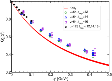
Figure 18: Result of $G_{E}(q^{2})$ with $t_{\rm sep}=12$, 14, and 16 on the $L=64$ lattice volume as a function of $q^{2}$. The data of $t_{\rm sep}=16$ are slightly shifted to the positive $x$ direction for clarity. Our previous result on the $L=128$ volume Shintani et al. (2019) given after taking average of three data sets calculated with $t_{\rm sep}=12$, 14 and 16 is also plotted by the asterisk symbol. The red curve represents Kelly’s parametrization of the experiment data Kelly (2004).

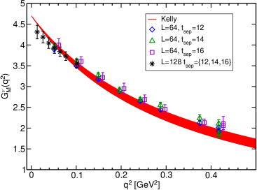
Figure 19: Same as Fig. 18 for $G_{M}(q^{2})$. The red curve represents Kelly’s parametrization of the experiment data Kelly (2004).

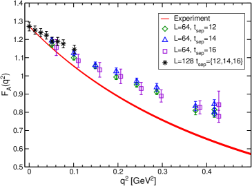
Figure 20: Same as Fig. 18 for $F_{A}(q^{2})$. The red curve is given by a dipole form with the dipole mass Bodek et al. (2008); Bernard et al. (2002) and $g_{A}$ Zyla et al. (2020).

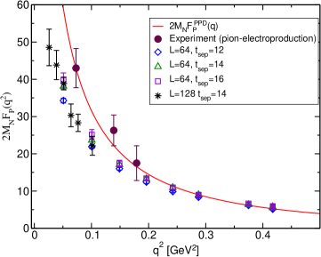
Figure 21: Same as Fig. 18 for $2M_{N}F_{P}(q^{2})$. The red curve is given by the pion-pole dominance model (PPD) $2M_{N}F_{P}^{\rm PPD}(q^{2})=4M_{N}^{2}F_{A}(q^{2})/(M_{\pi}^{2}+q^{2})$ with a dipole form of $F_{A}(q^{2})$ using the dipole mass Bodek et al. (2008); Bernard et al. (2002) and $g_{A}$ Zyla et al. (2020). The experimental result of the pion-electroproduction Choi et al. (1993) is also plotted by the diamond symbol.

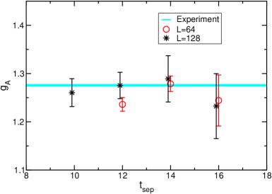
Figure 22: The renormalized $g_{A}$ from the $L=64$ and $L=128$ Shintani et al. (2019) lattices as a function of $t_{\rm sep}$. The data of $L=128$ are slightly shifted to the negative $x$ direction for clarity. The cyan band represents the experimental value Zyla et al. (2020).

Table 6: Results of the form factors with $t_{\rm sep}=12$.

$i$	$q_{i}^{2}\,[{\rm GeV}^{2}]$	$G_{E}(q^{2})$	$G_{M}(q^{2})$	$F_{A}(q^{2})$	$2M_{N}F_{P}(q^{2})$
0	0.000	1.0000	—	1.236(14)	—
1	0.051	0.8620(68)	3.899(63)	1.171(13)	34.29(64)
2	0.101	0.7569(70)	3.495(48)	1.100(13)	21.90(48)
3	0.149	0.6664(96)	3.175(53)	1.053(13)	16.00(34)
4	0.196	0.612(15)	2.900(52)	0.994(14)	12.42(36)
5	0.242	0.5570(80)	2.647(34)	0.952(13)	9.86(19)
6	0.288	0.4976(73)	2.442(38)	0.912(14)	8.35(22)
7	0.375	0.446(11)	2.125(60)	0.810(23)	6.15(21)
8	0.418	0.410(11)	2.018(56)	0.791(18)	5.22(21)
9	0.418	0.394(26)	1.928(64)	0.815(22)	5.14(26)

Table 7: Results of the form factors with $t_{\rm sep}=14$.

$i$	$q_{i}^{2}\,[{\rm GeV}^{2}]$	$G_{E}(q^{2})$	$G_{M}(q^{2})$	$F_{A}(q^{2})$	$2M_{N}F_{P}(q^{2})$
0	0.000	1.0000	—	1.279(16)	—
1	0.051	0.8616(74)	3.955(62)	1.194(15)	38.09(78)
2	0.101	0.763(10)	3.616(59)	1.125(15)	23.63(45)
3	0.149	0.6752(98)	3.277(60)	1.059(17)	17.09(42)
4	0.196	0.627(13)	2.920(52)	1.025(19)	13.27(35)
5	0.242	0.570(11)	2.689(52)	0.970(18)	10.93(40)
6	0.288	0.5082(86)	2.552(70)	0.937(21)	9.03(34)
7	0.375	0.452(24)	2.240(87)	0.834(25)	6.33(31)
8	0.418	0.406(17)	2.109(92)	0.801(22)	5.79(27)
9	0.418	0.419(27)	1.857(83)	0.845(24)	5.49(25)

Table 8: Results of the form factors with $t_{\rm sep}=16$.

$i$	$q_{i}^{2}\,[{\rm GeV}^{2}]$	$G_{E}(q^{2})$	$G_{M}(q^{2})$	$F_{A}(q^{2})$	$2M_{N}F_{P}(q^{2})$
0	0.000	1.0000	—	1.244(53)	—
1	0.051	0.880(18)	4.00(15)	1.155(44)	39.8(1.9)
2	0.101	0.774(18)	3.61(12)	1.083(36)	25.2(1.3)
3	0.149	0.685(19)	3.22(16)	1.033(40)	17.41(85)
4	0.196	0.623(27)	2.96(13)	0.997(40)	13.40(57)
5	0.242	0.552(20)	2.69(11)	0.931(34)	10.94(63)
6	0.288	0.510(17)	2.46(11)	0.890(33)	9.01(49)
7	0.375	0.429(19)	2.131(88)	0.827(36)	6.62(37)
8	0.418	0.405(18)	2.061(95)	0.778(33)	5.92(29)
9	0.418	0.399(72)	2.11(17)	0.842(74)	5.74(80)

Table 9: Fit results of $G_{E}(q^{2})$ with $t_{\rm sep}=14$ using dipole, quadratic, and z-expansion forms in Eqs. (18)–(20). The fit range is $q^{2}=q_{1}^{2}$–$q_{\rm cut}^{2}$. In all the fit we employ $G_{E}(0)=1$.

	dipole	quadratic	z-exp(cubic)
$\langle r_{E}^{2}\rangle$ [fm2]	0.646(16)	0.624(26)	0.737(62)
$\chi^{2}$/dof	1.7(0.9)	2.8(1.9)	1.3(0.9)
$q^{2}_{\rm cut}$ [GeV2]	0.418	0.242	0.418

Table 10: Fit results of $G_{M}(q^{2})$ with $t_{\rm sep}=14$ using dipole, quadratic, and z-expansion forms in Eqs. (18)–(20). The fit range is $q^{2}=q_{1}^{2}$–$q_{\rm cut}^{2}$. The fit result with a quadratic z-expansion form is also tabulated.

	dipole	quadratic	z-exp(cubic)	z-exp(quadratic)
$\mu$	4.357(42)	4.316(58)	3.53(28)	4.31(11)
$\langle r_{M}^{2}\rangle$ [fm2]	0.579(20)	0.489(17)	$-$2.1(1.1)	0.211(16)
$\chi^{2}$/dof	2.7(1.2)	2.1(1.2)	2.4(2.3)	1.0(1.4)
$q^{2}_{\rm cut}$ [GeV2]	0.418	0.418	0.288	0.242

Table 11: Fit results of $F_{A}(q^{2})/g_{A}$ with $t_{\rm sep}=14$ using dipole, quadratic, and z-expansion forms in Eqs. (18)–(20). The fit range is $q^{2}=q_{1}^{2}$–$q_{\rm cut}^{2}$. In all the fit we employ $F_{A}(0)/g_{A}=1$.

	dipole	quadratic	z-exp(cubic)
$\langle r_{A}^{2}\rangle$ [fm2]	0.308(17)	0.323(19)	0.337(39)
$\chi^{2}$/dof	0.4(0.9)	1.4(1.2)	1.6(1.5)
$q^{2}_{\rm cut}$ [GeV2]	0.149	0.288	0.288

References

- Pohl et al. (2010) R. Pohl et al., Nature 466, 213 (2010).
- Mohr et al. (2016) P. J. Mohr, D. B. Newell, and B. N. Taylor, Rev. Mod. Phys. 88, 035009 (2016), arXiv:1507.07956 [physics.atom-ph] .
- Karr et al. (2020) J.-P. Karr, D. Marchand, and E. Voutier, Nature Rev. Phys. 2, 601 (2020).
- Ishikawa et al. (2018) K.-I. Ishikawa, Y. Kuramashi, S. Sasaki, N. Tsukamoto, A. Ukawa, and T. Yamazaki, Phys. Rev. D98, 074510 (2018), arXiv:1807.03974 [hep-lat] .
- Shintani et al. (2019) E. Shintani, K.-I. Ishikawa, Y. Kuramashi, S. Sasaki, and T. Yamazaki, Phys. Rev. D 99, 014510 (2019), [Erratum: Phys.Rev.D 102, 019902 (2020)], arXiv:1811.07292 [hep-lat] .
- Alexandrou et al. (2017a) C. Alexandrou, M. Constantinou, K. Hadjiyiannakou, K. Jansen, C. Kallidonis, G. Koutsou, and A. Vaquero Aviles-Casco, Phys. Rev. D96, 034503 (2017a), arXiv:1706.00469 [hep-lat] .
- Alexandrou et al. (2017b) C. Alexandrou, M. Constantinou, K. Hadjiyiannakou, K. Jansen, C. Kallidonis, G. Koutsou, and A. Vaquero Aviles-Casco, Phys. Rev. D96, 054507 (2017b), arXiv:1705.03399 [hep-lat] .
- Gupta et al. (2017) R. Gupta, Y.-C. Jang, H.-W. Lin, B. Yoon, and T. Bhattacharya, Phys. Rev. D96, 114503 (2017), arXiv:1705.06834 [hep-lat] .
- Capitani et al. (2019) S. Capitani, M. Della Morte, D. Djukanovic, G. M. von Hippel, J. Hua, B. Jäger, P. M. Junnarkar, H. B. Meyer, T. D. Rae, and H. Wittig, Int. J. Mod. Phys. A 34, 1950009 (2019), arXiv:1705.06186 [hep-lat] .
- Green et al. (2017) J. Green, N. Hasan, S. Meinel, M. Engelhardt, S. Krieg, J. Laeuchli, J. Negele, K. Orginos, A. Pochinsky, and S. Syritsyn, Phys. Rev. D95, 114502 (2017), arXiv:1703.06703 [hep-lat] .
- Alexandrou et al. (2019) C. Alexandrou, S. Bacchio, M. Constantinou, J. Finkenrath, K. Hadjiyiannakou, K. Jansen, G. Koutsou, and A. Vaquero Aviles-Casco, Phys. Rev. D 100, 014509 (2019), arXiv:1812.10311 [hep-lat] .
- Bali et al. (2020) G. S. Bali, L. Barca, S. Collins, M. Gruber, M. Löffler, A. Schäfer, W. Söldner, P. Wein, S. Weishäupl, and T. Wurm (RQCD), JHEP 05, 126 (2020), arXiv:1911.13150 [hep-lat] .
- Jang et al. (2020a) Y.-C. Jang, R. Gupta, B. Yoon, and T. Bhattacharya, Phys. Rev. Lett. 124, 072002 (2020a), arXiv:1905.06470 [hep-lat] .
- Jang et al. (2020b) Y.-C. Jang, R. Gupta, H.-W. Lin, B. Yoon, and T. Bhattacharya, Phys. Rev. D 101, 014507 (2020b), arXiv:1906.07217 [hep-lat] .
- Alexandrou et al. (2021a) C. Alexandrou et al., Phys. Rev. D 103, 034509 (2021a), arXiv:2011.13342 [hep-lat] .
- Djukanovic et al. (2021) D. Djukanovic, T. Harris, G. von Hippel, P. M. Junnarkar, H. B. Meyer, D. Mohler, K. Ottnad, T. Schulz, J. Wilhelm, and H. Wittig, (2021), arXiv:2102.07460 [hep-lat] .
- Park et al. (2021) S. Park, R. Gupta, B. Yoon, S. Mondal, T. Bhattacharya, Y.-C. Jang, B. Joó, and F. Winter (Nucleon Matrix Elements (NME)), (2021), arXiv:2103.05599 [hep-lat] .
- Alexandrou et al. (2021b) C. Alexandrou, S. Bacchio, M. Constantinou, K. Hadjiyiannakou, K. Jansen, and G. Koutsou, (2021b), arXiv:2106.13468 [hep-lat] .
- Aglietti et al. (1994) U. Aglietti, G. Martinelli, and C. T. Sachrajda, Phys. Lett. B 324, 85 (1994), arXiv:hep-lat/9401004 .
- Bouchard et al. (2016) C. Bouchard, C. C. Chang, K. Orginos, and D. Richards, PoS LATTICE2016, 170 (2016), arXiv:1610.02354 [hep-lat] .
- Alexandrou et al. (2020) C. Alexandrou, K. Hadjiyiannakou, G. Koutsou, K. Ottnad, and M. Petschlies, Phys. Rev. D 101, 114504 (2020), arXiv:2002.06984 [hep-lat] .
- de Divitiis et al. (2012) G. M. de Divitiis, R. Petronzio, and N. Tantalo, Phys. Lett. B 718, 589 (2012), arXiv:1208.5914 [hep-lat] .
- Hasan et al. (2018) N. Hasan, J. Green, S. Meinel, M. Engelhardt, S. Krieg, J. Negele, A. Pochinsky, and S. Syritsyn, Phys. Rev. D97, 034504 (2018), arXiv:1711.11385 [hep-lat] .
- Ishikawa et al. (2019a) K. I. Ishikawa, N. Ishizuka, Y. Kuramashi, Y. Nakamura, Y. Namekawa, Y. Taniguchi, N. Ukita, T. Yamazaki, and T. Yoshie (PACS), Phys. Rev. D 99, 014504 (2019a), arXiv:1807.06237 [hep-lat] .
- Ishikawa et al. (2019b) K. I. Ishikawa, N. Ishizuka, Y. Kuramashi, Y. Nakamura, Y. Namekawa, E. Shintani, Y. Taniguchi, N. Ukita, T. Yamazaki, and T. Yoshié (PACS), Phys. Rev. D 100, 094502 (2019b), arXiv:1907.10846 [hep-lat] .
- Gockeler et al. (2005) M. Gockeler, T. R. Hemmert, R. Horsley, D. Pleiter, P. E. L. Rakow, A. Schafer, and G. Schierholz (QCDSF), Phys. Rev. D 71, 034508 (2005), arXiv:hep-lat/0303019 .
- Hagler et al. (2003) P. Hagler, J. W. Negele, D. B. Renner, W. Schroers, T. Lippert, and K. Schilling (LHPC, SESAM), Phys. Rev. D 68, 034505 (2003), arXiv:hep-lat/0304018 .
- Boyd et al. (1995) C. G. Boyd, B. Grinstein, and R. F. Lebed, Phys. Lett. B353, 306 (1995), arXiv:hep-ph/9504235 [hep-ph] .
- Hill and Paz (2010) R. J. Hill and G. Paz, Phys. Rev. D82, 113005 (2010), arXiv:1008.4619 [hep-ph] .
- Lellouch et al. (1995) L. Lellouch, J. Nieves, C. T. Sachrajda, N. Stella, H. Wittig, G. Martinelli, and D. G. Richards (UKQCD), Nucl. Phys. B 444, 401 (1995), arXiv:hep-lat/9410013 .
- Feng et al. (2020) X. Feng, Y. Fu, and L.-C. Jin, Phys. Rev. D 101, 051502 (2020), arXiv:1911.04064 [hep-lat] .
- Iwasaki (2011) Y. Iwasaki, (2011), UTHEP-118, arXiv:1111.7054 [hep-lat] .
- Taniguchi (2012) Y. Taniguchi, PoS LATTICE2012, 236 (2012), arXiv:1303.0104 [hep-lat] .
- Blum et al. (2013) T. Blum, T. Izubuchi, and E. Shintani, Phys.Rev. D88, 094503 (2013), arXiv:1208.4349 [hep-lat] .
- Shintani et al. (2015) E. Shintani, R. Arthur, T. Blum, T. Izubuchi, C. Jung, and C. Lehner, Phys. Rev. D91, 114511 (2015), arXiv:1402.0244 [hep-lat] .
- von Hippel et al. (2017) G. von Hippel, T. D. Rae, E. Shintani, and H. Wittig, Nucl. Phys. B914, 138 (2017), arXiv:1605.00564 [hep-lat] .
- Luscher (2004) M. Luscher, Comput.Phys.Commun. 156, 209 (2004), arXiv:hep-lat/0310048 [hep-lat] .
- Luscher (2007) M. Luscher, JHEP 0707, 081 (2007), arXiv:0706.2298 [hep-lat] .
- Ishikawa et al. (2016) K. I. Ishikawa, N. Ishizuka, Y. Kuramashi, Y. Nakamura, Y. Namekawa, Y. Taniguchi, N. Ukita, T. Yamazaki, and T. Yoshie (PACS), PoS LATTICE2015, 271 (2016), arXiv:1511.08549 [hep-lat] .
- Yamazaki et al. (2012) T. Yamazaki, K.-i. Ishikawa, Y. Kuramashi, and A. Ukawa, Phys. Rev. D 86, 074514 (2012), arXiv:1207.4277 [hep-lat] .
- Antognini et al. (2013) A. Antognini et al., Science 339, 417 (2013).
- Zyla et al. (2020) P. A. Zyla et al. (Particle Data Group), PTEP 2020, 083C01 (2020).
- Bernard et al. (2002) V. Bernard, L. Elouadrhiri, and U.-G. Meissner, J. Phys. G28, R1 (2002), arXiv:hep-ph/0107088 [hep-ph] .
- Bodek et al. (2008) A. Bodek, S. Avvakumov, R. Bradford, and H. S. Budd, Eur. Phys. J. C53, 349 (2008), arXiv:0708.1946 [hep-ex] .
- Sick (2018) I. Sick, Atoms 6, 2 (2018), arXiv:1801.01746 [nucl-ex] .
- Sasaki and Yamazaki (2008) S. Sasaki and T. Yamazaki, Phys. Rev. D78, 014510 (2008), arXiv:0709.3150 [hep-lat] .
- Bar (2019) O. Bar, Phys. Rev. D 99, 054506 (2019), arXiv:1812.09191 [hep-lat] .
- Kelly (2004) J. J. Kelly, Phys. Rev. C70, 068202 (2004).
- Choi et al. (1993) S. Choi et al., Phys. Rev. Lett. 71, 3927 (1993).