Electromagnetic Induction Imaging: Signal Detection Based on Tuned-Dressed Optical Magnetometry

Abstract

A recently introduced tuning-dressed scheme makes a Bell and Bloom magnetometer suited to detect weak variations of a radio-frequency (RF) magnetic field. We envisage the application of such innovative detection scheme as an alternative (or rather as a complement) to RF atomic magnetometers in electromagnetic-induction-imaging apparatuses.

I Introduction

In 2001, Griffiths griffiths_mst_01 proposed an imaging technique based on inferring one or more of the three passive electromagnetic properties (conductivity $\sigma$, permittivity $\epsilon$ and permeability $\mu$) to produce images on the basis of the response to a position dependent oscillating magnetic field. Several denominations are used to identify this kind of methodologies, among which electromagnetic induction imaging (EII) deans_apl_20 , electro-magnetic tomograhy (EMT) yu_el_93 , magnetic induction tomography (MIT) Korjenevsky_pm_00 ; bevington_as_20 , and also mutual inductance tomography (same acronym) soleimani_ieee_07 , the latter three stressing the potential of the technique to provide 3D mapping. A review on the subject was recently authored by Ma and Soleimani ma_mst_17 .

As a general feature, the technique uses an AC magnetic field to excite eddy currents in the specimen. The secondary magnetic field generated by those currents is then detected and analyzed.

Magnetometers can detect and record in-phase ($\epsilon$ dependent) and out-of-phase ($\sigma$ dependent) response of specimens subjected to an excitation radio-frequency field $B_{\mathrm{rf}}$. The response obtained while scanning the position of a sample with respect to the field generator and detector enables the registration of 2D maps. The possibility of varying the $B_{\mathrm{rf}}$ frequency (and correspondingly the skin depth in the specimen) enables 3D (tomographic) capabilities.

Optical magnetometers, in the so-called radio-frequency (RF) implementation deans_apl_16 ; wickenbrock_apl_16 are excellent detectors of weak (variation of) magnetic fields oscillating at a resonant frequency and hence constitute favourite detectors for EII, particularly in the case of low-conductivity and/or small size specimens.

This led recently to important steps toward high resolution EII of weakly conductive materials. Appositely developed RF magnetometers with opportune field-specimen arrangement, jensen_prr_19 ; marmugi_apl_19 , demonstrated a sensitivity sufficient to detect and characterize sub S m^-1 conductive material in small size ($5\text{\,}\mathrm{m}\mathrm{l}$) specimens, despite the operation in unshielded environment) deans_apl_20 .

Such specification level makes the technique suited to develop tools for medical diagnostics scharfetter_ieee_03 , where the negligible invasivity of EII represents a valuable attractive, but the low-conductivity and the need of high-spatial resolution constitute a severe requirement.

This work considers the potential of a peculiar configuration of a Bell&Bloom (BB) magnetometer as a detector of eddy currents induced in small and/or weakly conductive specimens, which could be eventually used to produce maps in 2D or 3D scans.

While the basic principle of operation (detection of a secondary magnetic field) is shared with the above mentioned research, the proposed sensor works with a particular arrangement that does not require resonant conditions for the time-dependent excitation field. The proposed arrangement can constitute an alternative as well as a complement to the commonly used RF magnetometers.

The standard BB implementation of atomic magnetometers is based on optically pumping atoms into a given Zeeman sublevel (typically with a maximum magnetic number along the quantization axis defined by the pump light wavevector) that is not stationary due to the presence of a transverse magnetic field.

In the usual picture of the BB operation, the macroscopic magnetization precesses around the magnetic field direction and it is periodically reinforced when its orientation is along the optical axis of the pump beam. The periodic reinforcement is obtained by modulating the pump radiation –its intensity, polarization or wavelength– synchronously with the precession. A weak and unmodulated probe radiation interrogates the evolution of the atomic state and produces an output signal whose dynamics is driven by the field under measurement.

The presence of time dependent field can modify the spin dynamics also in non-resonant conditions. As an example, in conventional BB magnetometry, slow-varying magnetic field variations, oriented along the bias field direction, are detected with a high sensitivity. Field variations along perpendicular directions produce some signal, as well, but with a second-order response biancalana_arx_21 .

Interesting dynamic responses of precessing spins are observed in a different regime, namely in the case of an intense fast-varying magnetic field. In particular, a strong magnetic field oscillating along the probe-beam axis (i.e. transversely to the static one) at a frequency much above the resonance may effectively freeze the atomic precession, according with a phenomenon originally studied in the late Sixties haroche_prl_1970 and generally known as magnetic dressing. .

In a recent work bevilacqua_prl_20 , we have demonstrated that the dressing phenomenon can be deeply tuned by the application of a secondary (and much weaker) field that oscillates at the same frequency –or at a low-order harmonic– of the dressing one, perpendicularly to the latter. Among the peculiarities of such tuned-dressed configuration, we pointed out that the system shows a remarkable response to small variations of the amplitude and/or of the phase of the tuning field. This work investigates with a proof-of-principle experiment the potential of such a tuning-dressing apparatus to detect tiny field variations due to eddy currents induced by the tuning field.

II Experimental setup

The experimental setup is built around a BB magnetometer making use of cesium thermal vapor in a centimetric, gas buffered cell. The atomic vapour is synchronously pumped by $D_{1}$ radiation (at $\text{\,}\mathrm{mW}\text{/}{\mathrm{cm}}^{2}$ irradiance) and polarimetrically probed by a weak (at $\text{\,}\mathrm{\SIUnitSymbolMicro W}\text{/}{\mathrm{cm}}^{2}$ irradiance) $D_{2}$ radiation, co-propagating with the pump one along the $x$ direction, further details can be found in Ref. biancalana_apb_16 .

The atomic sample is merged in a constant field at $\mu$T level (let its direction be $z$) oriented perpendicularly to the laser beams. This static field $B_{0}$ is obtained by partially compensating the environmental magnetic field. The task is accomplished by means of three large size (180 cm) mutually orthogonal Helmholtz pairs. Additional adjustable quadrupoles let improve the field homogeneity.

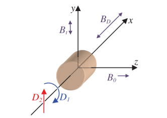
Figure 1: Magnetic field and laser beams geometry. Circularly polarized $D_{1}$ pump radiation and linearly polarized $D_{2}$ probe radiation propagate along $x$, which is the same direction of a strong oscillating (dressing) field $B_{D}$. A weaker (tuning) field $B_{t}$ oscillates along $y$ synchronously with $B_{D}$; a weak static field $B_{0}$ is oriented along $z$.

The tuning-dressing effect bevilacqua_prl_20 occurs when two phase-related oscillating fields ($B_{D}$ and $B_{t}$) are applied along $x$ to dress the atoms, and along $y$ to tune the dressing effect, respectively. A solenoidal coil ($11\text{\,}\mathrm{c}\mathrm{m}$ in length and $4\text{\,}\mathrm{c}\mathrm{m}$ in diameter) surrounding the cell generates $B_{D}$ and a small (millimetric) solenoid wound on a ferrite nucleus generates $B_{t}$. The interaction geometry is sketched in Fig.1.

The $B_{D}$ and $B_{t}$ coils are supplied by two waveform generators (Agilent 33250A) phase-locked to each other. Series capacitors help to adapt the impedances, and a linear amplifier can be used to enhance the $B_{t}$ amplitude. Each of these coils has $10\text{\,}\mathrm{O}\mathrm{h}\mathrm{m}$ series resistor to precisely monitor the current phases and amplitudes via a $16\text{\,}\mathrm{b}\mathrm{i}\mathrm{t}$, $500\text{\,}\mathrm{k}\mathrm{S}\mathrm{/}\mathrm{s}$ DAQ card (NI 6346).

The tuning-dressed phenomenon occurs and is well modeled and characterized for a tuning-field frequency $\omega_{t}$ that is an integer multiple of the dressing frequency $\omega_{D}$ ($\omega_{t}=p\omega_{D}$). It is worth stressing that, in the considered application, switching among different $p$ values may enable fast and relevant variations of the skin depth, which in EII applications may constitute an interesting feature.

The coil-specimen-sensor geometry is sketched in Fig.2. The used specimens are one or more Aluminum disks of assigned thickness $d$, diverse radii $R$, centered on the $y$ axis, and lying on a $xz$ plane between the $B_{t}$ generator and the atomic sensor. The experimental results reported in this work are obtained with $a=$$40\text{\,}\mathrm{m}\mathrm{m}$, $b=$$130\text{\,}\mathrm{m}\mathrm{m}$, $d=$$30\text{\,}\mathrm{\SIUnitSymbolMicro}\mathrm{m}$, and $D$ ranging from $24\text{\,}\mathrm{m}\mathrm{m}$ to $350\text{\,}\mathrm{m}\mathrm{m}$. In this proof-of-concept experiment, these values are chosen on the basis of fortuitous constraints of the available setup. In real imaging applications, all of them could be selected in view of optimizing the detection performance, in terms of sensitivity and/or spatial resolution.

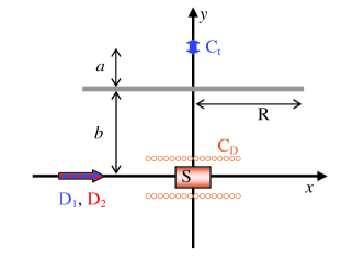
Figure 2: Relative positions of specimen, sensor, and tuning/dressing field sources. The specimen is a circular disk of radius R (thick grey line), which is parallel to the $xz$ plane and is centered on the $y$ axis, at a quote $y=b$ over the sensor $S$. A solenoidal coil $C_{D}$ surrounds $S$ and produces a homogeneous field $B_{D}$ along the $x$ axis. The latter coincides with the optical axis of the pump and probe lasers $D_{1}$ and $D_{2}$. A small dipolar source $C_{t}$ located on the y axis at distance $a$ from the specimen (and $a+b$ from the sensor) produces a tuning field $B_{t}$ which is oriented along $y$ on the sensor, and excites tangential eddy currents in the disk. Those currents modify both the amplitude and the phase of the tuning field on $S$.

The eddy currents induced in the conductive disks modify the amplitude and the phase of $B_{t}$ in the sensor location. As summarized in Sec.III, both these parameters play a role in shifting the effective Larmor frequency, and this is the key feature at the basis of the proposed detection technique.

III Effective Larmor Frequency

As shown and discussed in the Ref.bevilacqua_prl_20 , a magnetic field that oscillates in the direction perpendicular to both the transverse static field $B_{0}$ and the longitudinal dressing field $B_{D}$ at a frequency $p$ times larger than that of the dressing field, modifies the effective Larmor frequency according to

$$\Omega_{L}=\gamma\left[B_{0}J_{0}(\xi)+B_{t}J_{p}(\xi)\sin(\phi)\right],$$ (1)

if $p$ is an odd integer, and to

$$\Omega_{L}=\gamma\sqrt{\left[B_{0}J_{0}(\xi)\right]^{2}+\left[B_{t}J_{p}(\xi)\cos(\phi)\right]^{2}},$$ (2)

if it is an even one. Here, $\gamma$ is the atomic gyromagnetic factor ($\gamma\approx$$3.5\text{\,}\mathrm{Hz}\text{/}\mathrm{nT}$ for Cesium), and the argument $\xi$ is set by the amplitude of the dressing field $B_{D}$ and by its frequency $\omega_{D}$ according to

$$\xi=\frac{\gamma B_{D}}{\omega_{D}}.$$ (3)

The validity of the eqs.(1) and (2) requires that

$$\xi\gg\frac{\gamma B_{t}}{\omega_{D}},\frac{\omega_{0}}{\omega_{D}}$$

In the measurements shown in this paper, the tuning field oscillates at the same frequency of $B_{D}$ (i.e. $p=1$), while both its amplitude and phase vary either due to different waveform-generator settings or to the presence of conductive samples placed in the proximity of the field source and of the sensor. In particular assuming that $\phi=\varphi-\theta$, where $\varphi$ is the relative phase of the two RF generators, and $\theta$ is the dephasing caused by the eddy currents in the specimen, the effective Larmor frequency can be expressed as

$$f=\frac{\gamma}{2\pi}\left[J_{0}(\xi)B_{0}+J_{1}(\xi)B_{t}\sin{\phi}\right]=f_{0}+A\sin(\varphi-\theta),$$ (4)

where $f_{0}$ is the dressed frequency in absence of the tuning field. Beside causing the dephasing $\theta$, the eddy currents attenuate $B_{t}$, and this shielding effect determines a reduction of the parameter $A$.

The eq.(4) lets define the conditions in which the system response to either the attenuation or the dephasing is maximized:

$$\left|\frac{\partial f}{\partial A}\right|=\left|\sin(\varphi-\theta)\right|$$ (5)

is maximal for $\phi=\varphi-\theta=\pi/2$, while

$$\left|\frac{\partial f}{\partial\theta}\right|=\left|A\cos(\varphi-\theta)\right|$$ (6)

is maximal when $J_{1}$ is maximum, that is at $\xi\approx 1.84$ and $\phi=0,\pi$. These relations provide an indication of good experimental working conditions.

IV Results

The $B_{t}$ variation due to the eddy currents induced in the specimen can be evaluated analytically for large (infinite radius) disks dodd_jap_68 , or numerically for finite radius ones. The variation is monotonically dependent on the disk radius, and concerns both the phase and the amplitude of $B_{t}$. This is verified experimentally as shown in Fig.3

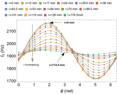
Figure 3: The resonance frequency as a function of the different relative phase $\varphi$, for various disk diameters whose size in mm is reported in the legend. The vertical error bar ($\approx$3\text{\,}\mathrm{Hz}\text{/}$$) is smaller than the symbols used in the graph. The solid lines represent the best fit profile obtained with the target function eq(4), with $A$ and $\theta$ as fitting parameters.

The atomic resonance is experimentally analyzed by scanning the frequency of the pump-laser modulation around the effective Larmor frequency expressed by the eq.(4). The resonance line-width is about 25 Hz, however the high S/N ratio let a best fit targeted to a Lorentzian profile determine the peak frequency with a sub-Hz accuracy. On the other hand, the ambient field fluctuations (the BB magnetometer is operated in an unshielded environment, with deactivated field-stabilization system biancalana_prapplml_19 ) are at nT level, and this leads to a few Hz uncertainty in the resonant frequency estimation.

The measurements shown here are performed at $B_{0}=$$1.7\text{\,}\mathrm{\SIUnitSymbolMicro T}\text{/}$ corresponding to an undressed Larmor frequency of $6\text{\,}\mathrm{kHz}\text{/}$. The dressing field frequency is set at $15\text{\,}\mathrm{kHz}\text{/}$ or $30\text{\,}\mathrm{kHz}\text{/}$, and its amplitude $B_{D}$ is set to get a dressing parameter $\xi=1.84$, according to the indication provided by the eq.(6). In these conditions, the dressed frequency with no tuning field, is $f_{0}=J_{0}(1.84)\gamma B_{0}/2\pi\approx$ $1900\text{\,}\mathrm{Hz}\text{/}$.

When the tuning field is activated, the measured peak frequency has a remarkable dependence on both the amplitude and the phase of $B_{t}$ at the sensor location, according to eq.(4). Both $A$ and $\theta$ can be determined by scanning the relative phase of the RF generators in the $[0,2\pi]$ interval.

The Fig.3 shows clearly that an increase in disk radius causes both a reduction of the amplitude $A$ and a phase shift of the sinusoidal profiles. It is also clear that larger variations of the effective Larmor frequency occur when $\phi=\pm\pi/2$, while operating near the zero-crossings ($\phi=0,\pi$) improves the sensitivity to $\phi$ (i.e to $\theta$) variations, consistently with the eqs.(5), (6).

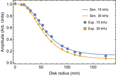
Figure 4: Dependence of the $B_{t}$ amplitude on the Al disk radius inferred from experimental measurements (dots) and evaluated from a simplified numerical simulation (line, see text for more details). Both the cases of $\omega_{D}=2\pi\cdot$$15\text{\,}\mathrm{k}\mathrm{H}\mathrm{z}$ and $2\pi\cdot$$30\text{\,}\mathrm{k}\mathrm{H}\mathrm{z}$ are considered. The thinner skin depth at $30\text{\,}\mathrm{k}\mathrm{H}\mathrm{z}$ produces a faster decay to a lower level, when the disk radius increases, as expected.

A clearer visualization is facilitated by a best fit procedure targeted to the function expressed in eq.4. Plots of the best-fit parameter $A$ versus the disk radius are shown with dots in Fig.4. The solid lines in that figure are results from a finite-elements numerical simulation. The latter is based on the geometry of Fig.2, without the $C_{D}$ solenoid and considering $B_{t}$ at the center of the sensor as produced by a point dipolar source and attenuated by on axis Al disks.

This analysis has been performed with the set of Al disks described in Sec.II and we report results obtained at both the tested tuning-dressing frequencies. Selecting different values of the oscillating fields changes the skin depth and hence modifies the shielding properties of the Al samples. As known, the skin depth depends on the absolute permeability $\mu$ of the medium and on its resistivity $\rho$, according to:

$$\delta=\sqrt{\frac{2\rho}{p\omega_{D}\mu}}$$ (7)

In the case of Al, this formula gives $\delta=$ $460\text{\,}\mathrm{\SIUnitSymbolMicro m}\text{/}$ and $650\text{\,}\mathrm{\SIUnitSymbolMicro m}\text{/}$, for the two considered frequencies, respectively. Both values are much larger than the thickness of the foil from which the Aluminum disks ($30\text{\,}\mathrm{\SIUnitSymbolMicro m}\text{/}$) are cropped.

The general trend of the experimental results reported in Fig.4 is qualitatively reproduced by numerical simulation. In particular both the experiment and the simulation show that the curve width and the asymptotic values decrease at higher $\omega_{D}$ (smaller $\delta$). However, some quantitative discrepancies emerge: double thickness Al disks are considered in the simulation to produce the well matching profiles reported in Fig.4. Indeed, several details are neglected in the simulation, such as the presence of the solenoid $C_{D}$ and of an electric heater surrounding the Cs cell, and the finite size of the $B_{t}$ source and of the sensor volume. Very likely one of more of these factors are responsible for the mentioned discrepancies. Similar issues are encountered in the phase estimations $\theta(r)$.

V Discussion

The proposed tuning-dressing technique, extends to all-optical atomic magnetometric sensors applicability as detectors in EII setups. Interestingly, the proposed arrangement could be easily implemented in pre-existing EII apparatuses, and dual modality (RF and tuning-dressing) setups could be built, with incremental complexity of the available instrumentation.

In arrangements where the pump and probe beams are not parallel, a dual-mode operation would make possible to apply the RF field along different orientation, in such a way to induce variously distributed eddy currents. In fact, while in RF magnetometry the RF field is applied perpendicularly to the pump beam, in the tuning-dressing BB arrangement $B_{t}$ is perpendicular to the probe beam.

Compared to conventional RF apparatuses, the tuning-dressing implementation besides not requiring that the detection field oscillates at a resonant frequency. Moreover, fast selection of different $B_{t}$ frequencies is feasible, via an appropriate selection of the harmonic parameter $p$. The possibility of selecting arbitrary values for both $\omega$ and $p$ is relevant for the skin depth dependence on $p\omega_{D}$ (eq. 7), which is of interest to improve the tomographic (three-dimensional) potential of the EII apparatuses.

Concerning the detection efficiency, the proposed methodology takes advantage from the fact that in the tuning-dressed configuration the weak tuning field borrows strength from the primary dressing field. The linear dependence on $B_{t}$ occurring for odd $p$ (which can be maximized with appropriate choices of $\xi$ and selecting $\phi=\pm\pi/2$) makes possible and efficient the use of approaches as that described in ref.deans_apl_20 . Specifically it would be possible to apply a vanishing $B_{t}$ obtained as a superposition of two opposite contributions, in such way that the specimen causes a $B_{t}$ variation via an unbalance of the two applied terms.

Improved detection techniques could be developed on the basis of the harmonic dependence on $\phi$. As an example, if $B_{t}$ oscillates at frequency $\omega_{t}$ slightly different from $p\omega$, the signal will appear as a low-frequency beating term oscillating at $\omega_{t}-p\omega$: a feature that would enable the application of phase-sensitive detection techniques.

VI Conclusion

We have presented a proof of principle experiment proposing a new kind of magnetometric detector of small or weakly conductive specimens. Specifically, we have used a recently studied dressing-field configuration to make an all-optical Bell-and-Bloom magnetometer suited to detect faint oscillating fields as occurring in magnetic induction tomography setups. The experiment demonstrated that the variation of a non-resonantly oscillating probe field can be effectively measured to detect the presence of conductive objects. The described approach can be regarded as non-resonant alternative to the well known methodologies based on RF magnetometers. It constitutes indeed a complementary approach to the problem and dual-mode (RF and tuning-dressing) apparatuses can be envisaged, with interesting novel features and enhanced flexibility.

References

- (1) H. Griffiths, “Magnetic induction tomography,” Measurement Science and Technology, vol. 12, pp. 1126–1131, jul 2001.
- (2) C. Deans, L. Marmugi, and F. Renzoni, “Sub-Sm–1 electromagnetic induction imaging with an unshielded atomic magnetometer,” Applied Physics Letters, vol. 116, no. 13, p. 133501, 2020.
- (3) Z. Z. Yu, A. T. Peyton, M. S. Beck, W. F. Conway, and L. A. Xu, “Imaging system based on electromagnetic tomography (EMT),” Electronics Letters, vol. 29, no. 7, pp. 625–626, 1993.
- (4) A. Korjenevsky, V. Cherepenin, and S. Sapetsky, “Magnetic induction tomography: experimental realization,” Physiological Measurement, vol. 21, pp. 89–94, feb 2000.
- (5) P. Bevington, R. Gartman, and W. Chalupczak, “Inductive imaging of the concealed defects with radio-frequency atomic magnetometers,” Applied Sciences, vol. 10, no. 19, 2020.
- (6) M. Soleimani, W. R. B. Lionheart, and A. J. Peyton, “Image reconstruction for high-contrast conductivity imaging in mutual induction tomography for industrial applications,” IEEE Transactions on Instrumentation and Measurement, vol. 56, no. 5, pp. 2024–2032, 2007.
- (7) L. Ma and M. Soleimani, “Magnetic induction tomography methods and applications: a review,” Measurement Science and Technology, vol. 28, p. 072001, jun 2017.
- (8) C. Deans, L. Marmugi, S. Hussain, and F. Renzoni, “Electromagnetic induction imaging with a radio-frequency atomic magnetometer,” Applied Physics Letters, vol. 108, no. 10, p. 103503, 2016.
- (9) A. Wickenbrock, N. Leefer, J. W. Blanchard, and D. Budker, “Eddy current imaging with an atomic radio-frequency magnetometer,” Applied Physics Letters, vol. 108, no. 18, p. 183507, 2016.
- (10) K. Jensen, M. Zugenmaier, J. Arnbak, H. Stærkind, M. V. Balabas, and E. S. Polzik, “Detection of low-conductivity objects using eddy current measurements with an optical magnetometer,” Phys. Rev. Research, vol. 1, p. 033087, Nov 2019.
- (11) L. Marmugi, C. Deans, and F. Renzoni, “Electromagnetic induction imaging with atomic magnetometers: Unlocking the low-conductivity regime,” Applied Physics Letters, vol. 115, no. 8, p. 083503, 2019.
- (12) H. Scharfetter, R. Casanas, and J. Rosell, “Biological tissue characterization by magnetic induction spectroscopy (mis): requirements and limitations,” IEEE Transactions on Biomedical Engineering, vol. 50, no. 7, pp. 870–880, 2003.
- (13) G. Bevilacqua, V. Biancalana, Y. Dancheva, A. Fregosi, and A. Vigilante, “Spin dynamic response to a time dependent field,” 2021.
- (14) S. Haroche, C. Cohen-Tannoudji, C. Audoin, and J. P. Schermann, “Modified Zeeman hyperfine spectra observed in 1H and 87Rb ground states interacting with a nonresonant RF field,” Phys. Rev. Lett., vol. 24, pp. 861–864, 1970.
- (15) G. Bevilacqua, V. Biancalana, A. Vigilante, T. Zanon-Willette, and E. Arimondo, “Harmonic fine tuning and triaxial spatial anisotropy of dressed atomic spins,” Phys. Rev. Lett., vol. 125, p. 093203, Aug 2020.
- (16) G. Bevilacqua, V. Biancalana, P. Chessa, and Y. Dancheva, “Multichannel optical atomic magnetometer operating in unshielded environment,” Applied Physics B, vol. 122, no. 4, p. 103, 2016.
- (17) C. V. Dodd and W. E. Deeds, “Analytical solutions to eddy-current probe-coil problems,” Journal of Applied Physics, vol. 39, no. 6, pp. 2829–2838, 1968.
- (18) G. Bevilacqua, V. Biancalana, Y. Dancheva, and A. Vigilante, “Self-adaptive loop for external-disturbance reduction in a differential measurement setup,” Phys. Rev. Applied, vol. 11, p. 014029, Jan 2019.