DCPT/21/14, DESY 21-107, IPPP/21/07, MCnet-21-13, SAGEX-21-16 Logarithmic corrections to the QCD component of
same-sign W-pair production for VBS studies

Abstract

We present the results of the first calculation of the logarithmic corrections to the QCD contribution to same-sign $W$-pair production, $pp\to e^{\pm}\nu_{e}\mu^{\pm}\nu_{\mu}jj$, for same-sign charged leptons. This includes all leading logarithmic contributions which scale as $\alpha_{W}^{4}\alpha_{s}^{2+k}\log^{k}(\hat{s}/p_{\perp}^{2})$. This process is important for the study of electroweak couplings and hence the QCD contributions are usually suppressed through a choice of Vector Boson Scattering (VBS) cuts. These select regions of phase space where logarithms in $\hat{s}/p_{\perp}^{2}$ are enhanced. While the logarithmic corrections lead to a small change for the cross sections, several distributions relevant for experimental studies are affected more significantly.

1 Introduction

Vector boson scattering (VBS) describes the process $pp\to VV+2j$ where each $V$ may be a $W$ or $Z$ boson. All possible $V^{*}V^{*}\to VV$ processes can be inserted between two quark lines to give this final state, e.g. figure 1(a), and it provides a key opportunity to study the mechanism of electroweak symmetry breaking, and in particular the means by which the Higgs boson unitarises $VV$-scattering. Other topologies may also contribute at this order, $\mathcal{O}(\alpha_{W}^{4})$ in the squared matrix element and the same final state may also be generated by gluon-exchange between the quark lines which contributes at $\mathcal{O}(\alpha_{W}^{2}\alpha_{s}^{2})$. There is also an interference channel between the two at $\mathcal{O}(\alpha_{W}^{3}\alpha_{s})$. Given the experimental importance of this process, next-to-leading order (NLO) QCD corrections to the different channels have been extensively studied [1, 2, 3, 4, 5, 6, 7, 8, 9] and matched with parton shower corrections [10, 11, 12, 13]. Calculations of NLO electroweak corrections [14] and combined NLO QCD and electroweak corrections are now also available [15, 16, 17, 18, 19]. See e.g. [20] for a recent review.

(a)                                                         (b)      a

Figure 1: Possible tree-level diagrams which contribute to $pp\to VVjj$ at (a) $\mathcal{O}(\alpha_{W}^{4})$ and (b) $\mathcal{O}(\alpha_{W}^{2}\alpha_{s}^{2})$ to the squared matrix element. Interference between the two contributes at $\mathcal{O}(\alpha_{W}^{3}\alpha_{s})$.

In order to cleanly study the electroweak (EW) processes of interest, analyses typically apply cuts which require a large invariant mass between two jets and/or a large rapidity separation between two jets [21, 22, 23]. These are very effective at enhancing the EW contributions over the QCD channels, but it is important to accurately predict the purity of the sample which remains. In particular, the requirement of large invariant mass or large rapidity separation enhances the importance of logarithmic corrections of the form $\log(\hat{s}/p_{t}^{2})$ which arise at all orders of $\alpha_{s}$ (the leading logarithmic (LL) corrections scale as $\alpha_{s}^{k+2}\log^{k}(\hat{s}/p_{t}^{2})$). The combination $\alpha_{s}\log(\hat{s}/p_{t}^{2})$ is not necessarily small in these regions of phase space so that the logs can damage the convergence of the perturbative expansion. This means that the very cuts which suppress the QCD contribution make it harder to calculate a reliable estimate of that contribution.

Similar cuts are applied to separate the electroweak vector boson fusion (VBF) and QCD gluon fusion (GF) components in vector boson fusion analyses of $pp\to H+2j$. In this case, predictions including all LL corrections and matched to fixed order are available within the HEJ framework [24, 25, 26, 27]. Further, that framework also allows the inclusion of finite quark-mass effects for arbitrary jet multiplicities [28] which is currently only available at LO up to 3-jets. Here it was seen that while the inclusive cross sections for GF were in good agreement between the LL predictions of HEJ and fixed-order calculations at NLO, significant differences in the invariant-mass and rapidity distributions lead to a large difference in the predicted cross sections after cuts on invariant-mass and rapidity-separation were applied. At NLO, the impact of requiring $|\Delta y_{j_{1}j_{2}}|>2.8$ and $m_{j_{1}j_{2}}>400$ GeV reduced the cross section to 9% of the inclusive value while at LL with finite quark masses, the impact of the same cuts reduced the cross section to 4% of the corresponding inclusive value, indicating the cuts were roughly a factor of two more effective. This behaviour is largely due to the dominance of the $gg$-component within the inclusive cuts, and the difference in the $m_{jj}$-spectrum of the $gg$, $qg$ and $qq$ components[29, 30]. The same behaviour has also been seen in other comparisons between combinations of fixed-order, parton shower and HEJ predictions, e.g. [31, 32, 33].

Given the identical type of cuts usually applied to the jets when studying VBS to those in VBF, one would expect the impact of adding LL corrections to also be significant in this process. In this paper, we calculate the $\alpha_{s}^{k}\log^{k}(\hat{s}/p_{t}^{2})$ corrections to the $\mathcal{O}(\alpha_{W}^{2}\alpha_{s}^{2})$ component of VBS. We do this within the HEJ framework. These could then be straight-forwardly combined with predictions for electroweak channels to give a complete description of $pp\to W^{\pm}W^{\pm}+\geq 2j$, for example using the method described in [17]. This was done previously for $pp\to W+2j$ in [34] where LL predictions of the QCD component from HEJ were combined with electroweak predictions from Powheg+Pythia [35, 36, 37, 38] and were found to describe data very well, especially at large invariant mass.

In the following section, we outline how LL accuracy is obtained in the predictions from HEJ and then focus on how to construct the necessary amplitudes to describe $pp\to W^{\pm}W^{\pm}+\geq 2j$ at this order. In section 3, we illustrate the impact of the LL corrections on distributions which are typically studied at the LHC, both before and after VBS cuts are applied. We conclude in section 4.

2 Construction of Leading-Logarithm Amplitudes

2.1 Logarithmic Accuracy

The Born-level scattering amplitudes for the same-sign $W$-pair production process ${pp\to W^{\pm}W^{\pm}+\geq 2j}$ depicted in figure 1(b) can be expanded in powers of $\hat{s}/p_{t}^{2}$ considered in the limit of large $\hat{s}\to\infty$ with fixed $p_{\perp j_{1}}\sim p_{\perp j_{2}}\sim p_{\perp}$, where $p_{\perp}$ is an arbitrary (but fixed) transverse scale. In this limit, large $\hat{s}$ with fixed $p_{\perp}$ is reached by increasing rapidity differences between the jets. For processes permitting a gluon (colour-octet) exchange between the two jets (which the production of a same-sign $W$-pair does), this expansion of $|\mathcal{M}|^{2}$ starts at $\alpha_{s}^{2}\hat{s}^{2}/p_{\perp}^{4}$.

The leading logarithmic corrections to the cross section are controlled by the scattering amplitudes in this so-called Multi-Regge Kinematic limit, where the invariant mass between each pair of coloured particles is large but the transverse scales are fixed. The higher-order corrections to the cross section for these processes will contain terms of $\alpha_{s}\log(\hat{s}/p_{t}^{2})$[39, 40, 41], and such corrections have traditionally been resummed through the use of the formalism developed by Balitskii, Fadin, Kuraev and Lipatov[42].

The all-order, leading logarithmic accuracy in $\log(\hat{s}/p_{t}^{2})$ is ensured by a systematic control of the power-expansion to $\hat{s}/(p_{t}^{2})^{n}$ of $|\mathcal{M}|^{2}$ of each real correction with $n$ legs, and the expansion into terms of $(\alpha_{s}\log(\hat{s}/p_{t}))^{n}$ of the virtual corrections, with subtraction terms organising the cancellation of divergences between real and virtual corrections. In order to control just the leading logarithmic corrections to the Born-level process, one needs to consider just the leading expansion in $\hat{s}/p_{t}^{2}$ of each multiplicity, and its virtual corrections. This leading term in the expansion in $\hat{s}/p_{t}^{2}$ has contributions only from processes which allow a colour octet exchange between each particle considered in order of increasing rapidity. So processes with the rapidity ordering (or equivalently light-cone momentum ordering in the MRK limit) $qQ\to Qq$ (incoming and outgoing states ordered in light-cone momentum, and dropping the $W$s from the listing, since their ordering is irrelevant for the discussion) will not contribute at leading order in the expansion, whereas the leading order term will receive contributions from the same partonic process with the states ordered as $qQ\to qQ$.

For states of higher multiplicity, the leading contribution is from orderings such as $qQ\to qgQ$, which permit a colour octet (gluon, spin-1) exchange between each parton considered in the ordering of rapidity. The orderings $qQ\to gqQ$ require a colour singlet (spin-$\frac{1}{2}$) exchange between the $gq$. The contribution to the square of the scattering amplitudes in the MRK limit is then suppressed by one power of $\hat{s}$ compared to the contribution from the ordering $qQ\to qgQ$. This power suppression of the amplitude leads to a logarithmic suppression of the contribution to the cross section (see e.g. [43, 26, 44]).

The factorisation of the scattering amplitudes in the MRK limit[40, 43] implies that the MRK limit of these amplitudes can be constructed to the required accuracy in $s/(p_{t}^{2})^{n}$ using building blocks which depend on a reduced set of the momenta. The cross section can be calculated to leading logarithmic accuracy using an amplitude consisting of so-called impact factors, describing the forward and backward particle production, and a Lipatov vertex describing the production of a gluon of central rapidity. The Lipatov vertex depends on the momenta of the incoming and outgoing quarks, and the emitted gluon. The impact factor depends on the momenta of the incoming quark $p_{a}$, the outgoing quark $p_{1}$ and the $W$ (or its decay products) only. These impact factors are in fact the same as those used for single $W$ production in association with dijets[24, 45]. The cross sections discussed in the current study will be matched to full fixed-order accuracy of high multiplicity (up to 6 jets), see section 2.3. Earlier studies have shown that with such high-multiplicity matching, the overall impact of sub-leading logarithmic contributions on two and three-jet observables is very minor indeed. Therefore we will in this study calculate to just leading logarithmic accuracy, matched to high multiplicity fixed order.

2.2 Amplitudes for $pp\to W^{\pm}W^{\pm}+\geq 2j$ Within HEJ

In this subsection we present the new amplitudes required to apply the HEJ method to the process $pp\to W^{\pm}W^{\pm}+\geq 2j$. At this point we include the leptonic decay of the $W$ bosons as we will need this to compute predictions for typical experimental cuts and analyses. As described in the previous subsection, for a given multiplicity, a HEJ amplitude is built out of impact factors and Lipatov vertices. These multiplicities are then combined with the Lipatov ansatz for virtual corrections in order to achieve leading logarithmic accuracy in $\hat{s}/p_{t}^{2}$ at all orders in $\alpha_{s}$.

We begin with the impact factors which are independent of the number of gluons in the amplitude and hence can be derived from the lowest order process where they occur. The starting point is therefore the leading order (LO) process:

$$q(p_{a})Q(p_{b})\to(W_{1}^{\pm}\to)\ell(p_{\ell_{1}})\bar{\ell}(p_{\bar{\ell}_{1}})(W_{2}^{\pm}\to)\ell^{\prime}(p_{\ell_{2}})\bar{\ell}^{\prime}(p_{\bar{\ell}_{2}})q^{\prime}(p_{1})Q^{\prime}(p_{2}),$$ (1)

where $q$ and $Q$ represent different quark or anti-quark flavours. There are eight Feynman diagrams which contribute at LO, each similar to figure 1(b), which arise from the $qq^{\prime}W$ vertices for each boson being assigned to different points on different quark lines.

We define the following current to describe the production of a $W$ boson from a quark line with an off-shell gluon, $q(p_{i})\to(W\to\ell\bar{\ell})q^{\prime}(p_{o})g^{*}$:

$$\begin{split}j^{W}_{\mu}(p_{i},p_{o},p_{\ell},p_{\bar{\ell}})=&\ \frac{g_{W}^{2}}{2}\ \frac{1}{(p_{\ell}+p_{\bar{\ell}})^{2}-m_{W}^{2}+i\Gamma_{W}m_{W}}\ \left[\bar{u}^{-}(p_{\ell})\gamma_{\alpha}v^{-}(p_{\bar{\ell}})\right]\\ &\times\left(\frac{\bar{u}^{-}(p_{o})\gamma^{\alpha}(\not{p}_{o}+\not{p}_{\ell}+\not{p}_{\bar{\ell}})\gamma_{\mu}u^{-}(p_{i})}{(p_{o}+p_{\ell}+p_{\bar{\ell}})^{2}}+\frac{\bar{u}^{-}(p_{o})\gamma_{\mu}(\not{p}_{i}-\not{p}_{\ell}-\not{p}_{\bar{\ell}})\gamma^{\alpha}u^{-}(p_{i})}{(p_{i}-p_{\ell}-p_{\bar{\ell}})^{2}}\right),\end{split}$$ (2)

as illustrated in figure 2.

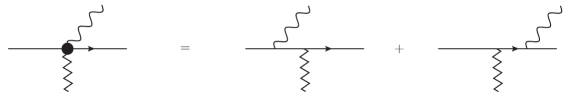
Figure 2: Schematic illustration of the current, $j^{W}_{\mu}(p_{i},p_{o},p_{\ell},p_{\bar{\ell}})$, defined in Eq. (2) to describe the production of a $W$ boson from a quark line with an off-shell gluon (shown as a zigzag line).

The exact tree-level result can then be compactly expressed as the following two contractions of two such currents:

$$\begin{split}i\mathcal{M}^{\rm HEJ,tree}=g_{s}^{2}&\left(\frac{j_{\mu}^{W}(p_{a},p_{1},p_{\ell_{1}},p_{\bar{\ell}_{1}})g^{\mu\nu}j_{\nu}^{W}(p_{b},p_{2},p_{\ell_{2}},p_{\bar{\ell}_{2}})}{q^{2}}\right.\\ &\left.\qquad\qquad+\ \frac{j_{\mu}^{W}(p_{a},p_{1},p_{\ell_{2}},p_{\bar{\ell}_{2}})g^{\mu\nu}j_{\nu}^{W}(p_{b},p_{2},p_{\ell_{1}},p_{\bar{\ell}_{1}})}{\tilde{q}^{2}}\right),\end{split}$$ (3)

where $q=p_{a}-p_{1}-p_{\ell_{1}}-p_{\bar{\ell}_{1}}$ and $\tilde{q}=p_{a}-p_{1}-p_{\ell_{2}}-p_{\bar{\ell}_{2}}$. This amplitude remains exact at $\mathcal{O}(\alpha_{W}^{2}\alpha_{s})$ within the HEJ framework. In particular, our full amplitudes already achieve LO accuracy without the need for further matching with the exception of channels with identical leptons or quarks. The extra contributions arising in these special cases are suppressed in the MRK limit and do not affect the logarithmic accuracy. They are nonetheless included through the fixed-order matching described in the next subsection.

In order to achieve LL accuracy in the inclusive predictions, we supplement the tree-level amplitude with corrections arising from real and virtual corrections at $\alpha_{s}^{3}$ and above. Although separately divergent in $4d$, we follow the procedure outlined in [24, 46] to arrive at a finite amplitude for $qQ\to W^{\pm}W^{\pm}q^{\prime}g...gQ^{\prime}$ for any number of intermediate gluons. It is built from [24]:

• a skeleton function for the process (often the LO matrix-element), given by a contraction of impact factors

• a Lipatov vertex, $V^{\mu}$, for each real gluon emission with transverse momentum above scale $\lambda_{cut}$,

• finite exponential factors for each $t$-channel propagator which arise from the sum of the virtual corrections at LL (given by the Lipatov Ansatz) and integration over all unresolved real emissions with $p_{t}<\lambda_{cut}$.

We typically choose values of $\lambda_{cut}$ to be around 0.2 GeV, and have checked that our final results (cross sections and distributions) are not strongly dependent on this value. We have compared results for the total cross section at values of $\lambda_{cut}$ between 0.2 GeV and 2 GeV and observe discrepancies of a few percent at most, with no clear trend. This is a non-trivial check that the implementation is correct.

The construction above is built around the concept of effective $t$-channel momentum (although far more than contributions from $t$-channel diagrams are included). These are the momenta which would correspond to a planar $t$-channel diagram when the outgoing coloured particles are ordered in rapidity. For $qQ\to W^{\pm}W^{\pm}q^{\prime}g...gQ^{\prime}$, it is already clear at lowest order that there is not a unique definition of a $t$-channel momentum, as it depends on the pairing of $W$ bosons with quark lines (see Eq. (3)). However, the addition of extra gluons does not make this problem any worse than at leading order, and hence for any number of coloured particles in the final state there will be two sets of planar $t$-channels. We will keep both (and the interference between them) which significantly complicates the expressions compared to the HEJ description of single-$W$ production [45]. It is similar to the treatment of $pp\to Z+2j$ in HEJ [46]. Specifically, we write the amplitude using two skeleton functions, each with its own tower of real and virtual corrections. Interference between these is immediately included upon squaring the amplitude.

These skeleton functions are defined as

$$\begin{split}B&=j_{\mu}^{W}(p_{a},p_{1},p_{\ell_{1}},p_{\bar{\ell}_{1}})g^{\mu\nu}j_{\nu}^{W}(p_{b},p_{n},p_{\ell_{2}},p_{\bar{\ell}_{2}}),\\ \tilde{B}&=j_{\mu}^{W}(p_{a},p_{1},p_{\ell_{2}},p_{\bar{\ell}_{2}})g^{\mu\nu}j_{\nu}^{W}(p_{b},p_{n},p_{\ell_{1}},p_{\bar{\ell}_{1}}),\end{split}$$ (4)

which relate to the two possible combinations of leptons and quark lines. These have corresponding planar $t$-channel momenta:

$$\begin{split}q_{1}&=p_{a}-p_{1}-p_{\ell_{1}}-p_{\bar{\ell}_{1}},\qquad q_{i}=q_{i-1}-p_{i}\quad i=2,...,n-1,\\ \tilde{q}_{1}&=p_{a}-p_{1}-p_{\ell_{2}}-p_{\bar{\ell}_{2}},\qquad\tilde{q}_{i}=\tilde{q}_{i-1}-p_{i}\quad i=2,...,n-1.\end{split}$$ (5)

We refer to the corresponding momenta-squared as $t_{i}=q_{i}^{2}$ and $\tilde{t}_{i}=\tilde{q}_{i}^{2}$ for $i=1,...,n-1$. We also define the rapidity differences of consecutive quarks/gluons to be $\Delta y_{i}=y_{i+1}-y_{i}$. The LL accurate matrix element is then given by

$$\begin{split}&|\mathcal{M}^{\rm HEJ,reg}_{qQ\to W_{1}^{\pm}W_{2}^{\pm}q^{\prime}(n-2)gQ^{\prime}}|^{2}\\ =&\ g_{s}^{4}\frac{C_{F}}{8N_{c}}\ (g_{s}^{2}C_{\!A})^{n-2}\ \\ &\times\Bigg{(}\frac{|B|^{2}}{t_{1}t_{(n-1)}}\exp(\omega^{0}(q_{(n-1)\perp})\Delta y_{n-1})\prod^{n-2}_{i=1}\frac{-V^{2}(q_{i},q_{(i+1)})}{t_{i}t_{(i+1)}}\exp(\omega^{0}(q_{i\perp})\Delta y_{i})\\ &\quad+\ \frac{|\tilde{B}|^{2}}{\tilde{t}_{1}\tilde{t}_{(n-1)}}\exp(\omega^{0}(\tilde{q}_{(n-1)\perp})\Delta y_{n-1})\prod^{n-2}_{i=1}\frac{-V^{2}(\tilde{q}_{i},\tilde{q}_{(i+1)})}{\tilde{t}_{i}\tilde{t}_{(i+1)}}\exp(\omega^{0}(\tilde{q}_{i\perp})\Delta y_{i})\\ &\quad+\ \frac{2\Re\{B\tilde{B}\}}{\sqrt{t_{1}\tilde{t}_{1}}\sqrt{t_{(n-1)}\tilde{t}_{b(n-1)}}}\exp(\omega^{0}(\sqrt{q_{(n-1)\perp}\tilde{q}_{(n-1)\perp}})\Delta y_{n-1})\\ &\hskip 85.35826pt\;\times\prod^{n-2}_{i=1}\frac{-V(q_{i},q_{(i+1)})\cdot V(\tilde{q}_{i},\tilde{q}_{(i+1)})}{\sqrt{t_{i}\tilde{t}_{i}}\sqrt{t_{(i+1)}\tilde{t}_{(i+1)}}}\exp(\omega^{0}(\sqrt{q_{i\perp}\tilde{q}_{i\perp}})\Delta y_{i})\Bigg{)},\end{split}$$ (6)

where

$$\begin{split}V^{\mu}(q_{1},q_{2})&=-(q_{1}+q_{2})^{\mu}+\frac{p_{a}^{\mu}}{2}\left(\frac{q_{1}^{2}}{p\cdot p_{a}}+\frac{p\cdot p_{b}}{p_{a}\cdot p_{b}}+\frac{p\cdot p_{n}}{p_{a}\cdot p_{n}}\right)+p_{a}\leftrightarrow p_{1},\\ &\qquad-\frac{p_{b}^{\mu}}{2}\left(\frac{q_{2}^{2}}{p\cdot p_{b}}+\frac{p\cdot p_{a}}{p_{a}\cdot p_{b}}+\frac{p\cdot p_{1}}{p_{b}\cdot p_{1}}\right)-p_{b}\leftrightarrow p_{n}\qquad{\rm{for}}\ p=q_{1}-q_{2},\\ \omega^{0}(q_{\perp})&=-\frac{g_{s}^{2}C_{\!A}}{4\pi^{2}}\log\left(\frac{q_{\perp}^{2}}{\lambda_{cut}^{2}}\right).\end{split}$$ (7)

One can immediately check that at $\mathcal{O}(\alpha_{W}^{4}\alpha_{s}^{2})$ this exactly agrees with the summed, averaged and squared amplitude of Eq. (3). One can extend this test to higher orders by comparing the result of Eq. (6) with the virtual corrections removed (i.e. setting $\omega^{0}(q_{\perp}^{2})=0$) at a fixed order in $\alpha_{s}$ to the corresponding LO result. In the MRK limit, these should match. We illustrate this in figure 3 for squared matrix elements for sample channels at $\alpha_{W}^{4}\alpha_{s}^{3}$ and $\alpha_{W}^{4}\alpha_{s}^{4}$.

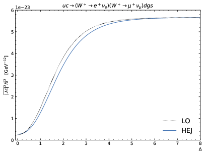
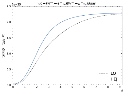
(a)                                                              (b)

Figure 3: Phase space explorer plots for $uc\to W^{+}W^{+}+n\textrm{ jets}$ for (a) 3 jets and (b) 4 jets.

The rapidities of the outgoing particles in these slices are:

(a)	$y_{d}=y_{e}=y_{\nu_{e}}=\Delta,\ y_{s}=y_{\mu}=y_{\nu_{\mu}}=-\Delta,\ y_{g}=0$,
(b)	$y_{d}=y_{e}=y_{\nu_{e}}=\Delta,\ y_{s}=y_{\mu}=y_{\nu_{\mu}}=-\Delta,\ y_{g_{1}}=\Delta/3,\ y_{g_{2}}=-\Delta/3$.

The rapidity separation of the quarks and gluons is controlled by the parameter $\Delta$ and hence the MRK limit is approached at the right-hand side of the plots. The other parameters used are given in Appendix A, but the behaviour seen is not sensitive to the exact values of the transverse momentum or the azimuthal angles. In both plots, we show the squared matrix element divided by $\hat{s}^{2}$, to achieve a finite non-zero value in the MRK limit. The exact LO result (black, dotted line) and the approximation within HEJ (solid, red line) are very similar throughout the range and converge to the same limiting value at large $\Delta$. The plots also show the rich dynamics of the matrix elements which would be missed at small values of $\Delta$ if the limiting value was used throughout phase space.

The LL accurate cross section is then given by the following sum over multiplicities and integration over all phase space (where $\ell_{l}$ numbers the four leptons from the $W$ decays):

$$\begin{split}\sigma^{\rm LL}_{pp\to W^{\pm}W^{\pm}+2j}=&\sum_{f_{i1},f_{i2}}\ \sum_{n=2}^{\infty}\ \prod_{i=1}^{n}\left(\int\frac{\mathrm{d}^{2}\mathbf{p}_{i\perp}}{(2\pi)^{3}}\ \int\frac{\mathrm{d}y_{i}}{2}\right)\ \prod_{l=1}^{4}\left(\int\frac{\mathrm{d}^{2}\mathbf{p}_{\ell_{l}\perp}}{(2\pi)^{3}}\ \int\frac{\mathrm{d}y_{\ell_{l}}}{2}\right)\\ &\times\frac{\overline{\left|\mathcal{M}^{\rm HEJ,reg}_{qQ\to W_{1}^{\pm}W_{2}^{\pm}q^{\prime}(n-2)gQ^{\prime}}\right|}^{2}}{\hat{s}^{2}}\\ &\times\ \ x_{a}f_{A,f_{i1}}(x_{a},Q_{a})\ x_{2}f_{B,f_{i2}}(x_{b},Q_{b})\ (2\pi)^{4}\ \delta^{2}\!\!\left(\sum_{k=1}^{n}\mathbf{p}_{k\perp}+\sum_{m=1}^{4}\mathbf{p}_{\ell_{m}\perp}\right)\ \mathcal{O}_{2j}(\{p_{j}\}).\end{split}$$ (8)

We emphasise here that no approximation is made to the phase space being integrated over, only within the matrix element itself. This integral can be efficiently implemented in an exclusive Monte Carlo event generator giving full flexibility to implement experimental cuts and distributions. Before this integration, we first multiply the squared matrix element by reweighting factors to implement fixed-order accuracy, as discussed in the next section.

2.3 Matching to Fixed Order

In the previous subsection, we have described how to construct the cross section for $pp\to W^{\pm}W^{\pm}+\geq 2j$ at LL accuracy in $\hat{s}/p_{t}^{2}$. In order to increase the validity of the approach, we will supplement this with subleading terms which will provide leading-order accuracy at each order in $\alpha_{s}$, up to the point where this is computationally feasible. For this process, in this study, that is samples with 2, 3, 4, 5 and 6 jets at LO. We observe that the impact of adding higher multiplicity fixed-order samples decreases with each multiplicity, and in particular that the $6$-jet sample has at most a few percent effect in any distribution so we are confident that our results have converged.

The matching is then implemented using the methods of HEJ2 [27] which reorganises the integral over phase space to supplement fixed-order samples at each order with real and virtual corrections such that leading-logarithmic accuracy is maintained at all orders in $\alpha_{s}$ and additionally leading-order accuracy is achieved for the $n$-jet components for $n=2$–$6$. This method is implemented in the exclusive event generator, HEJ2 [47], which is publicly available at https://hej.hepforge.org. The process $pp\to W^{\pm}W^{\pm}+\geq 2j$ will be included in a future public release of HEJ2. The fixed-order input is given as Les Houches events and can be taken from any generator. In this study we have used Sherpa [48] to generate the fixed-order input.

Finally, we rescale all the final HEJ2 predictions to match the total cross section to the inclusive NLO cross section for each scale choice. However, for the setup described in section 3, and as discussed there, this turns out to have a negligible impact in this case.

3 Impact of Leading-Logarithm Corrections

We will now show the predictions constructed and matched as described in the previous section for observables commonly studied at the LHC for the process $pp\to W^{\pm}W^{\pm}+\geq 2j$, where one $W^{\pm}$ decays in the electron channel and one in the muon channel. We will compare these with an NLO calculation of the same process (here taken from Sherpa [48] using COMIX [49] with the extension of OpenLoops [50]) to assess the impact of the new LL corrections. Also included for comparison is a calculation including MC@NLO matching [51] with the shower generator CS Shower [52] packaged with Sherpa. We use the NNPDF3.0 NLO PDF set [53] as provided by LHAPDF6 [54]. We choose the central factorisation and renormalisation scale as the geometric mean of the transverse momenta of the two leading jets, $\mu_{F}=\mu_{R}=\sqrt{p_{\perp;j_{1}}p_{\perp;j_{2}}}$. These scales are varied independently by a factor of two around this central value, with the constraint that their ratio is kept between 0.5 and 2. The uncertainty bands shown in the plots are obtained from the envelope of these variations.

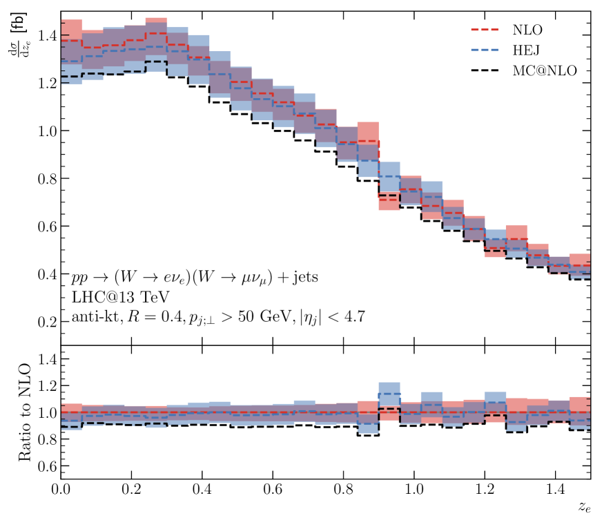
(a)

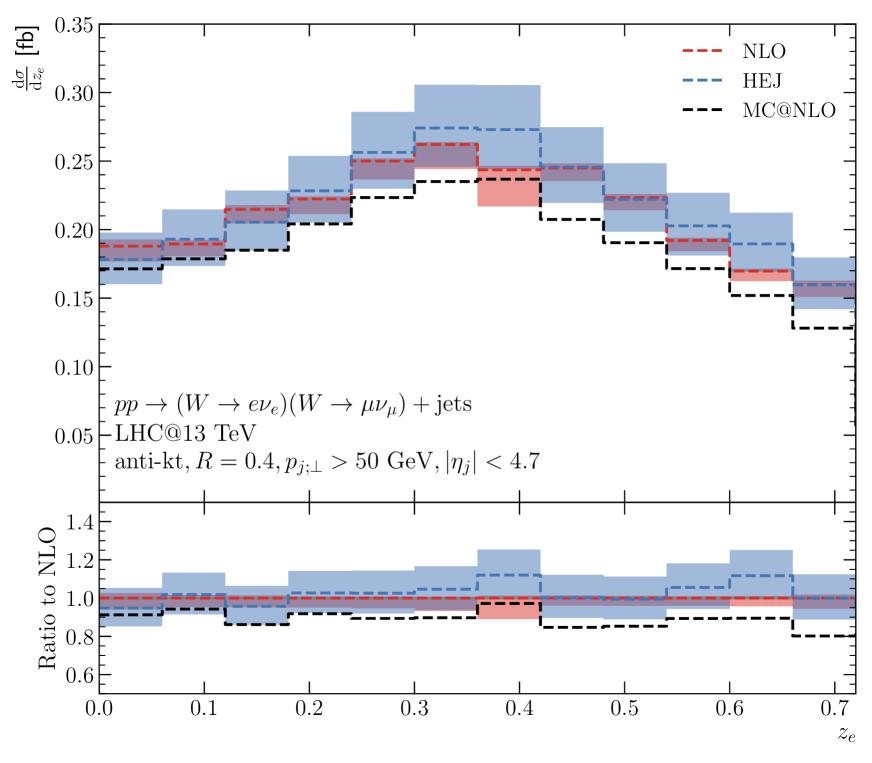
(b)

Figure 9: The differential distribution in the Zeppenfeld variable for the electron in $pp\to W^{\pm}W^{\pm}+\geq 2j$, without and with additional VBS cuts.

In figures 5–9 we show distributions measured in a recent CMS analysis [22]. It is not meaningful to compare to the data points in that study as these include the large $\mathcal{O}(\alpha_{W}^{4})$ contributions. The cuts applied to the predictions are listed in Table 1. Those in the first group form the inclusive cuts which are applied to all plots. The additional three criteria (below the second horizontal line) give the extra cuts on leading dijet invariant mass, leading jet pseudorapidity separation and the Zeppenfeld variable [55]

$$z_{l}=\frac{\eta_{l}-\frac{1}{2}(\eta_{j_{1}}+\eta_{j_{2}})}{|\eta_{j_{1}}-\eta_{j_{2}}|},$$ (9)

where $j_{1}$ and $j_{2}$ are the two hardest jets in the event. These cuts are used to try to suppress the QCD contribution to this process. We will refer to them as “VBS cuts” and will show results before and after these extra criteria. The output of HEJ is exclusive in the momenta of all outgoing particles. Here we have used the functionality of linking HEJ directly with Rivet[56] to apply the cuts and fill the histograms.

Variable	Selection Cut
Lepton pseudorapidity	$|\eta_{l}|<2.5$
Jet pseudorapidity	$|\eta_{j}|<4.7$
Leading/subleading lepton $p_{\textrm{T}}$	$p_{T}>25/20$ GeV
Missing transverse momentum	$E^{\textrm{miss}}_{\textrm{T}}>30$ GeV
Jet $p_{\textrm{T}}$	$p_{\textrm{T}}>50$ GeV
Lepton isolation	$\Delta R(l,\textrm{jet})>0.4$ o/w jet is removed
Di-lepton mass	$m_{ll}>20$ GeV
Di-lepton mass restriction	$|m_{ll}-m_{Z}|>15$ GeV
Di-jet mass	$m_{j_{1}j_{2}}>500$ GeV
Jet rapidity separation	$|\Delta\eta_{j_{1}j_{2}}|>2.5$
Max lepton Zeppenfeld variable (Eq. 9)	$\max(z_{l})<0.75$

Table 1: The selection cuts used in the analysis where the lepton cuts apply only to the charged leptons. The last three rows define the additional VBS cuts.

Before discussing the distributions, we give the cross sections obtained at NLO, with MC@NLO and with HEJ2 before and after the application of VBS cuts in Table 2 for the central scale choice above. Both before and after VBS cuts the values are remarkably similar for the central value of the renormalisation and factorisation scales. This is a marked difference to other processes where similar cuts have been applied. For example in $pp\to H+\geq 2j$ despite relative agreement at the inclusive level, the HEJ2 predictions were significantly more suppressed by VBF cuts than those at NLO (by about a factor of 2) [28]. This result is sensitive to the scale choice; in the window of variations we studied, the ratio between the HEJ2 and NLO cross sections varies by as much as 22% in either direction. It is also clear from the distributions that follow that this agreement is not flat in phase space (even for the central scale choice), but arises from different regions where the HEJ2 result is greater and less than NLO.

Cross Section (fb)	without VBS cuts, $\sigma_{\rm incl}$	with VBS cuts, $\sigma_{\rm VBS}$	$\sigma_{\rm VBS}$/$\sigma_{\rm incl}$
HEJ2 $W^{+}W^{+}$	$1.428\pm 0.002$	$0.1219\pm 0.0004$	$0.0854\pm 0.0003$
NLO $W^{+}W^{+}$	$1.41\pm 0.05$	$0.12\pm 0.07$	$0.08\pm 0.02$
MC@NLO $W^{+}W^{+}$	$1.285\pm 0.003$	$0.1033\pm 0.0006$	$0.0804\pm 0.0005$
HEJ2 $W^{-}W^{-}$	$0.6586\pm 0.0003$	$0.0402\pm 0.0001$	$0.0610\pm 0.0002$
NLO $W^{-}W^{-}$	$0.68\pm 0.02$	$0.04\pm 0.01$	$0.06\pm 0.02$
MC@NLO $W^{-}W^{-}$	$0.6186\pm 0.0004$	$0.0371\pm 0.0002$	$0.0600\pm 0.0002$

Table 2: This table gives the total cross section calculated with the new HEJ2 LO+LL predictions in this paper compared to the result at NLO accuracy, both before and after the VBS cuts given in the text.

In figure 4, we show the exclusive jet rates. For only the inclusive selection criteria, we see a steady decrease at each multiplicity, but in the HEJ2 predictions the $4$-, $5$- and $6$-jet rates remain at 21%, 6% and 2% of the exclusive $2$-jet rate respectively. After VBS cuts, the relative importance of the higher multiplicity rates in the HEJ2 predictions is enhanced with the $2$-jet and $3$-jet rates being very similar and the $4$-, $5$- and $6$-jet rates now increasing to 40%, 13% and 3% of the exclusive $2$-jet rate respectively. In the NLO sample after VBS cuts, the $3$-jet rate is a third larger than the $2$-jet rate for the central scale choice. The scale variation bands here are very large; however, for any one choice the $3$-jet was always comparable to or greater than the $2$-jet rate. This is already one measure of the importance of the higher-order corrections in $\alpha_{s}$ (i.e. $\alpha_{s}^{4}$ and above). The MC@NLO predictions shows that the effect of adding a parton shower to the NLO predictions is to distribute the $3$-jet component among the higher jet-rate bins. The large contribution to the cross section from events with three or more jets suggests that additional jet vetoes could be used to further suppress the relative QCD contribution to $pp\to VV+2j$.

The jet rate plots are affected by the lepton isolation cut (see table 1). Any jet which satisfies $\Delta R(l,\textrm{jet})<0.4$ for any charged lepton is removed from the event, but the event is still kept provided there are at least two further jets. This means that events which arise from a theoretical calculation with e.g. 4 jets can appear in the plot in the 2-jet or 3-jet bin. For comparison, we show the equivalent plots from HEJ2 without lepton isolation applied in appendix C.

(a)

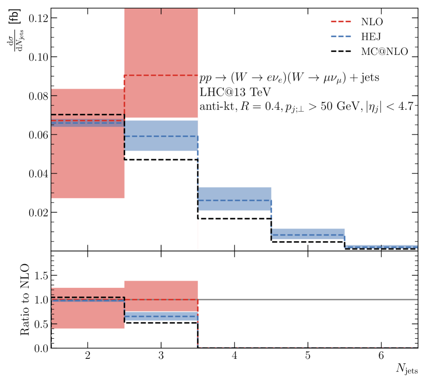
(b)

Figure 4: Exclusive jet rates for $pp\to W^{\pm}W^{\pm}+\geq 2j$, (a) without and (b) with additional VBS cuts.

Figure 5 shows the comparison for the difference in pseudorapidity between the two leading jets. Here we see only modest differences in shape between the two descriptions which are slightly enhanced once VBS cuts are applied in the right-hand plot. However, any differences lie mostly within the scale variation bands. Here, and in the remaining distributions, we observe only a small impact of adding a parton shower to the pure NLO calculation, with no significant changes in shapes of distributions.

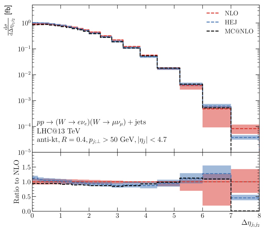
(a)

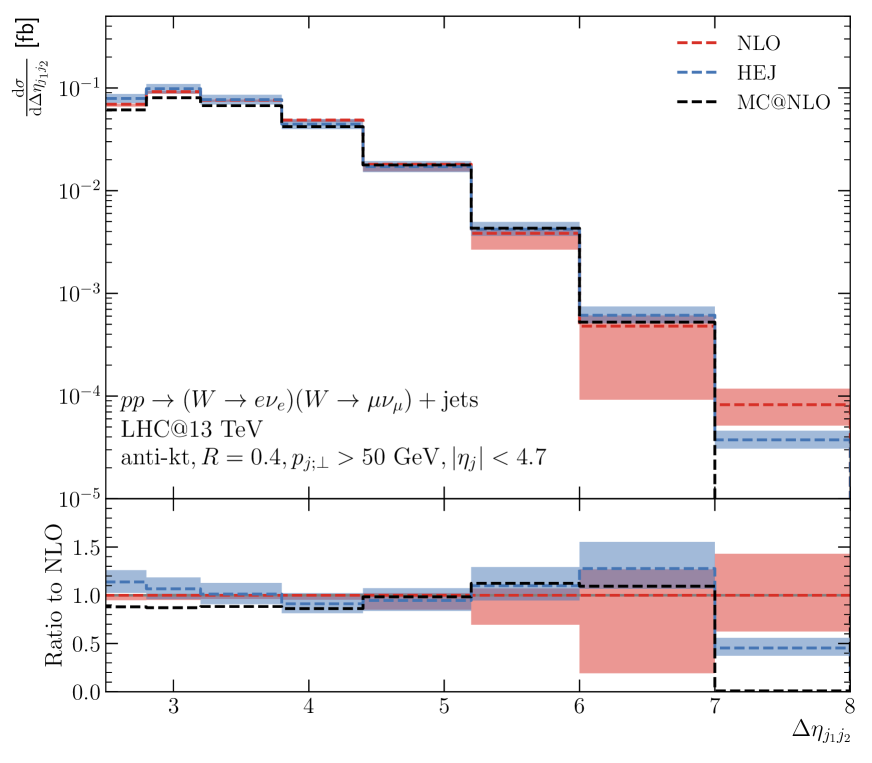
(b)

Figure 5: The differential distribution in the pseudorapidity separation of the two leading jets in $pp\to W^{\pm}W^{\pm}+\geq 2j$, (a) without and (b) with additional VBS cuts.

Figure 6 exhibits greater differences in shape in the distribution of the transverse momentum of the leading jet. For the inclusive cuts in (a), the HEJ2 prediction starts much lower than the NLO prediction but increases with respect to it until the predictions cross around 200 GeV. Above this value the prediction from HEJ2 falls more slowly leading to a prediction of a harder spectrum in $p_{j_{1};\perp}$. A very similar behaviour is seen in (b) after the application of VBS cuts. This distribution clearly emphasises that the close agreement of the total cross section values is a coincidence of the experimental setup used. If the transverse momentum requirement of the jets had been larger, the HEJ2 cross section would have also been correspondingly larger than that from NLO.

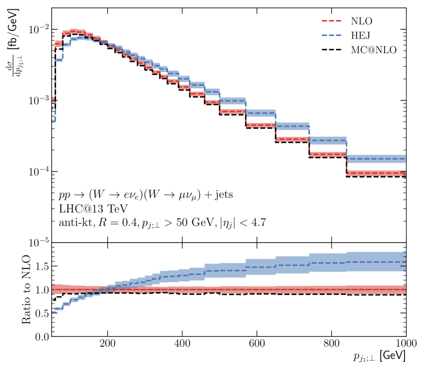
(a)

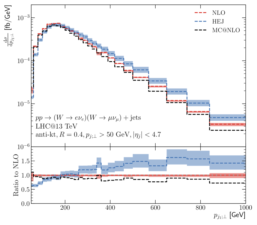
(b)

Figure 6: The differential distribution in the transverse momentum of the hardest jet in $pp\to W^{\pm}W^{\pm}+\geq 2j$, (a) without and (b) with additional VBS cuts.

Similarly, in figure 7 we see that the HEJ2 and NLO predictions for the invariant mass distribution of the two leading jets have a different shape with a ratio which increases steadily from 0.5 at $m_{j_{1}j_{2}}=0$ GeV to 1.4 by $m_{j_{1}j_{2}}=2$ TeV where it roughly plateaus. A similar effect is seen after VBS cuts are imposed, although of course here the lower region has been removed. The point where the predictions cross has moved to a slightly higher value of $m_{j_{1}j_{2}}$ as a result of the cuts on the other variables which form part of the VBS cuts.

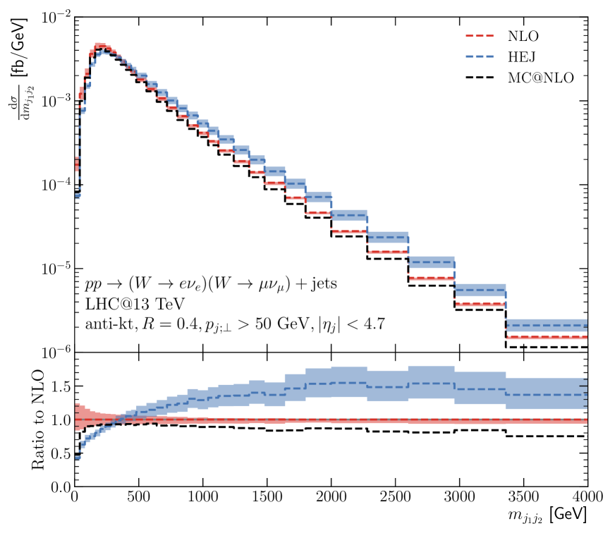
(a)

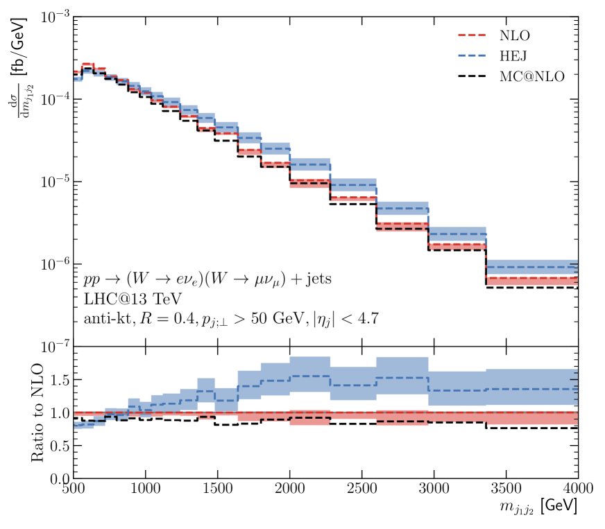
(b)

Figure 7: The differential distribution in the invariant mass of the two leading jets in $pp\to W^{\pm}W^{\pm}+\geq 2j$, (a) without and (b) with additional VBS cuts.

In figure 8, we show the distributions in the invariant mass of the two charged leptons from the decays of the $W$ bosons. This is related to the invariant mass of the jets if one considers event topologies where the $W$ bosons follow the direction of the associated quark lines. For modest transverse momenta, the invariant mass between particles is driven by their rapidity difference. The leptons, though, are required to be more central than the jets and we see more modest differences between the NLO and HEJ2 predictions.

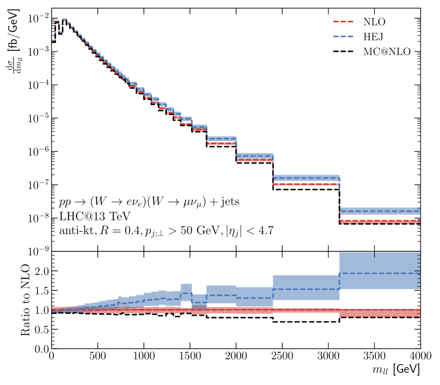
(a)

(b)

Figure 8: The differential distribution in the invariant mass of the two charged leptons in $pp\to W^{\pm}W^{\pm}+\geq 2j$, (a) without and (b) with additional VBS cuts.

The final distribution we show in this section is the Zeppenfeld variable $z_{e}$ of the electron, defined in Eq. (9). This measures the relative position of the electron in these events with respect to the jet system. Both before and after VBS cuts, the predictions from NLO and from HEJ2 are in very close agreement, and the ratio between the two remains largely flat throughout the region showing that this variable is largely insensitive to the logarithmic corrections at higher orders in $\alpha_{s}$.

In this section, we have compared the new predictions for $pp\to e^{\pm}\nu_{e}\mu^{\pm}\nu_{\mu}+\geq 2j$ available in HEJ2 (which include the leading logarithmic corrections in $\hat{s}/p_{\perp}^{2}$ at all orders in $\alpha_{s}$) with those obtained at next-to-leading order in QCD. We have seen close agreement in the total cross sections obtained in the two approaches at the central scale choice, but a study of distributions in $p_{j_{1};\perp}$, $m_{j_{1}j_{2}}$ and $m_{ll}$ show large differences in shape which make this agreement appear to be a coincidence of the specific values chosen in the experimental cuts.

4 Conclusions

We have presented the calculation of all leading logarithmic contributions which scale as
$\alpha_{W}^{4}\alpha_{s}^{k+2}\log^{k}(\hat{s}/p_{t}^{2})$ to the production of a same-sign $W$-pair which decays leptonically, i.e. the QCD contribution to the process $pp\to e^{\pm}\nu_{e}\mu^{\pm}\nu_{\mu}+\geq 2j$. In order to separate the electroweak and QCD contributions to this process, so-called VBS cuts are usually applied to require large invariant mass and rapidity separation of the tagging jets. These cuts exactly select regions of phase space where the logarithms above become important. The equivalent corrections have been seen to be significant in the QCD component of $pp\to H+\geq 2j$ through vector boson fusion, where similar cuts are used. To assess their impact in $pp\to e^{\pm}\nu_{e}\mu^{\pm}\nu_{\mu}+\geq 2j$, we have compared our new predictions to those obtained at NLO within the experimental setup of a recent 13 TeV CMS analysis.

We have found that the HEJ2 cross section is very close to the NLO prediction both for inclusive cuts, and after VBS cuts have been applied. However, it is clear from the distributions that this agreement arises from cancellations across phase space rather than being true throughout. The distributions in transverse momentum of the leading jet in figure 6, in invariant mass of the leading jets in figure 7 and in invariant mass of the charged leptons in figure 8 show clear differences in shape with differences of up to 50% between HEJ2 and NLO. There are other distributions, $\Delta\eta_{j_{1}j_{2}}$ and $z_{e}$ where the two sets of predictions show close agreement, indicating that these distributions are more stable with respect to higher-order logarithmic corrections.

Previous studies of this process have seen that the $3$-jet component is significant in typical experimental analyses, enhanced within VBS cuts. We also find this, and that it extends beyond $3$-jets. The exclusive jet components within HEJ2 are matched to leading-order accuracy for $2$–$6$ jets. We showed in figure 4 that the VBS cuts do indeed increase the significance of the $3$–$6$-jet components relative to the $2$-jet component. The contribution from $3$-jets is similar to $2$-jet in HEJ2 and greater than the $2$-jet at NLO. The $4$–$6$-jet components steadily decrease but such that the $6$-jet components still contributed at the order of a few percent in some distributions.

We therefore conclude that logarithmic corrections of the form $\alpha_{W}^{4}\alpha_{s}^{k+2}\log^{k}(\hat{s}/p_{t}^{2})$ are numerically significant at the 13 TeV LHC, and should be included in accurate modelling of the QCD background to vector boson scattering.

Appendix A Momentum Configurations for Phase Space Slices

We give here the momentum configurations used for the plots of the matrix elements in figure 3. For the 3 jet final state in figure 3(a), we use:

$$\begin{split}p_{i}&=p_{i;\perp}(\cos(\phi_{i}),\sin(\phi_{i}),\sinh(y_{i}),\cosh(y_{i}))\\ p_{d;\perp}&=p_{\ell;\perp}=p_{g;\perp}=40\textrm{ GeV}\\ p_{\nu_{\ell};\perp}&=\frac{m_{W}^{2}}{2p_{\ell;\perp}\left(\cosh\left(y_{\ell}-y_{\nu_{\ell}}\right)-\cos\left(\phi_{\ell}-\phi_{\nu_{\ell}}\right)\right)}\\ p_{s;\perp}&=-(p_{d;\perp}+p_{e;\perp}+p_{\nu_{e};\perp}+p_{\mu;\perp}+p_{\nu_{\mu};\perp}+p_{g;\perp})\\ \phi_{d}&=2\pi/3,\quad\phi_{e}=\pi/4,\quad\phi_{\mu}=-\pi/2,\quad\phi_{\nu_{e}}=-\pi/4,\quad\phi_{\nu_{\mu}}=+\pi/2,\quad\phi_{g}=0.4\\ y_{d}&=y_{e}=y_{\nu_{e}}=\Delta,\quad y_{s}=y_{\mu}=y_{\nu_{\mu}}=-\Delta,\quad y_{g}=0\end{split}$$ (10)

For the 4 jet final state in figure 3(b) we use:

$$\begin{split}p_{i}&=p_{i;\perp}(\cos(\phi_{i}),\sin(\phi_{i}),\sinh(y_{i}),\cosh(y_{i}))\\ p_{d;\perp}&=p_{\ell;\perp}=p_{g_{1};\perp}=p_{g_{2};\perp}=40\textrm{ GeV}\\ p_{\nu_{\ell};\perp}&=\frac{m_{W}^{2}}{2p_{\ell;\perp}\left(\cosh\left(y_{\ell}-y_{\nu_{\ell}}\right)-\cos\left(\phi_{\ell}-\phi_{\nu_{\ell}}\right)\right)}\\ p_{s;\perp}&=-(p_{d;\perp}+p_{e;\perp}+p_{\nu_{e};\perp}+p_{\mu;\perp}+p_{\nu_{\mu};\perp}+p_{g_{1};\perp}+p_{g_{2};\perp})\\ \phi_{d}&=\pi,\quad\phi_{e}=\pi/4,\quad\phi_{\mu}=-\pi/2,\quad\phi_{\nu_{e}}=-\pi/4,\quad\phi_{\nu_{\mu}}=+\pi/2,\quad\phi_{g_{1}}=\pi/2,\quad\phi_{g_{2}}=-\pi/3\\ y_{d}&=y_{e}=y_{\nu_{e}}=\Delta,\quad y_{s}=y_{\mu}=y_{\nu_{\mu}}=-\Delta,\quad y_{g_{1}}=\Delta/3,\quad y_{g_{2}}=-\Delta/3\end{split}$$ (11)

The qualitative effects seen in figure 3 are only sensitive to the rapidity values (and not to the exact choices of transverse momenta or azimuthal angle).

Appendix B Simulation Parameters

In Table 3 we summarise the parameters used to generate the predictions in section 3.

Variable	Value
PDF	NNPDF30_nlo_as_0118 (lhapdf number 260000)
$m_{Z}$	91.1876 GeV
$\Gamma_{Z}$	2.4952 GeV
$m_{W}$	80.385 GeV
$\Gamma_{W}$	2.085 GeV
$\mu_{F}$	$\sqrt{p_{\perp;j_{1}}p_{\perp;j_{2}}}$
$\mu_{R}$	$\sqrt{p_{\perp;j_{1}}p_{\perp;j_{2}}}$
$\alpha_{s}(m_{Z})$	0.118 (set to match PDF)
$1/\alpha_{w}$	132.232
$G_{F}$	$1.16639\times 10^{-5}\ \textrm{GeV}^{-2}$
Sherpa Version	2.2.2
Openloops Version	1.3.1
Parton Shower	CS Shower (packaged with Sherpa)

Table 3: The input parameters used for the plots in section 3.

Sherpa uses the complex mass scheme for vector boson masses and $\alpha_{w}$ is calculated in the $G_{\mu}$ scheme from these.

Appendix C Exclusive Jet Rates Without Lepton Isolation Requirement

In figure 4 we showed the exclusive jet rates obtained at NLO and with HEJ2 for the experimental setup described in Table 1. This includes a lepton isolation requirement where any jet which satisfies $\Delta R(l,{\rm jet})<0.4$ is removed from the event. This means that many events appear in bins with lower numbers of jets than that present in the calculation of the weight of that event. To more closely reflect the impact of the higher orders in the calculation, in figure 10 we show the jet rates from HEJ2 with the lepton isolation requirement removed (all other cuts remain the same).

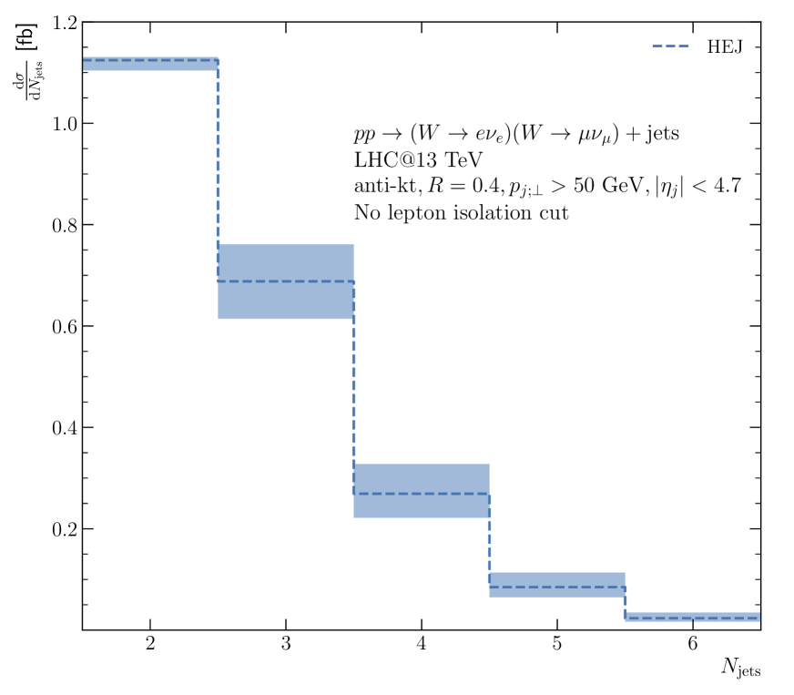
(a)

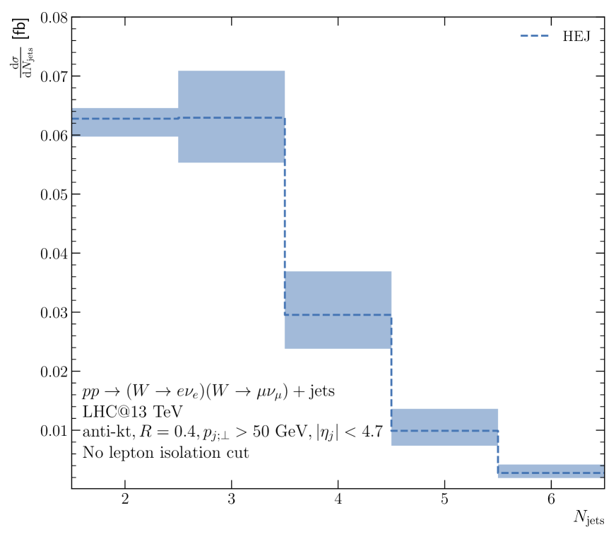
(b)

Figure 10: Exclusive jet rates for $pp\to W^{\pm}W^{\pm}+\geq 2j$ as in figure 4 except now the lepton isolation requirement has been removed, (a) without and (b) with additional VBS cuts.

The differences with only inclusive cuts are modest, with a slight decrease in the first bin and slight increases in the higher bins. After VBS cuts, the effect is more pronounced. The $3$-jet rate is now slightly above the $2$-jet rate and there is then a bigger step down to the $4$, $5$ and $6$ jet rates which have each risen slightly from the values after lepton isolation cuts. They are now 47%, 16% and 4% respectively of the exclusive $2$-jet rate compared to 40%, 13% and 3% after the lepton isolation cut is applied.

References

- [1] C. Oleari and D. Zeppenfeld, QCD corrections to electroweak nu(l) j j and l+ l- j j production, Phys. Rev. D 69 (2004) 093004, [hep-ph/0310156].
- [2] B. Jäger, C. Oleari and D. Zeppenfeld, Next-to-leading order QCD corrections to W+W- production via vector-boson fusion, JHEP 07 (2006) 015, [hep-ph/0603177].
- [3] B. Jäger, C. Oleari and D. Zeppenfeld, Next-to-leading order QCD corrections to Z boson pair production via vector-boson fusion, Phys. Rev. D 73 (2006) 113006, [hep-ph/0604200].
- [4] G. Bozzi, B. Jäger, C. Oleari and D. Zeppenfeld, Next-to-leading order QCD corrections to W+ Z and W- Z production via vector-boson fusion, Phys. Rev. D 75 (2007) 073004, [hep-ph/0701105].
- [5] B. Jäger, C. Oleari and D. Zeppenfeld, Next-to-leading order QCD corrections to W+ W+ jj and W- W- jj production via weak-boson fusion, Phys. Rev. D 80 (2009) 034022, [0907.0580].
- [6] T. Melia, K. Melnikov, R. Röntsch and G. Zanderighi, Next-to-leading order QCD predictions for production at the LHC, JHEP 12 (2010) 053, [1007.5313].
- [7] A. Denner, L. Hosekova and S. Kallweit, NLO QCD corrections to W+ W+ jj production in vector-boson fusion at the LHC, Phys. Rev. D 86 (2012) 114014, [1209.2389].
- [8] F. Campanario, M. Kerner, L. D. Ninh and D. Zeppenfeld, Next-to-leading order QCD corrections to and production in association with two jets, Phys. Rev. D 89 (2014) 054009, [1311.6738].
- [9] J. Baglio et al., Release Note - VBFNLO 2.7.0, 1404.3940.
- [10] T. Melia, P. Nason, R. Röntsch and G. Zanderighi, plus dijet production in the POWHEGBOX, Eur. Phys. J. C 71 (2011) 1670, [1102.4846].
- [11] B. Jäger and G. Zanderighi, NLO corrections to electroweak and QCD production of W+W+ plus two jets in the POWHEGBOX, JHEP 11 (2011) 055, [1108.0864].
- [12] B. Jäger, A. Karlberg and G. Zanderighi, Electroweak production in the Standard Model and beyond in the POWHEG-BOX V2, JHEP 03 (2014) 141, [1312.3252].
- [13] B. Jager, A. Karlberg and J. Scheller, Parton-shower effects in electroweak production at the next-to-leading order of QCD, Eur. Phys. J. C 79 (2019) 226, [1812.05118].
- [14] B. Biedermann, A. Denner and M. Pellen, Large electroweak corrections to vector-boson scattering at the Large Hadron Collider, Phys. Rev. Lett. 118 (2017) 261801, [1611.02951].
- [15] B. Biedermann, A. Denner and M. Pellen, Complete NLO corrections to W+W+ scattering and its irreducible background at the LHC, JHEP 10 (2017) 124, [1708.00268].
- [16] A. Denner, S. Dittmaier, P. Maierhöfer, M. Pellen and C. Schwan, QCD and electroweak corrections to WZ scattering at the LHC, JHEP 06 (2019) 067, [1904.00882].
- [17] M. Chiesa, A. Denner, J.-N. Lang and M. Pellen, An event generator for same-sign W-boson scattering at the LHC including electroweak corrections, Eur. Phys. J. C 79 (2019) 788, [1906.01863].
- [18] A. Denner, R. Franken, M. Pellen and T. Schmidt, NLO QCD and EW corrections to vector-boson scattering into ZZ at the LHC, JHEP 11 (2020) 110, [2009.00411].
- [19] A. Denner, R. Franken, M. Pellen and T. Schmidt, Full NLO predictions for vector-boson scattering into Z bosons and its irreducible background at the LHC, 2107.10688.
- [20] R. Covarelli, M. Pellen and M. Zaro, Vector-Boson scattering at the LHC: Unraveling the electroweak sector, Int. J. Mod. Phys. A 36 (2021) 2130009, [2102.10991].
- [21] ATLAS collaboration, M. Aaboud et al., Observation of electroweak production of a same-sign boson pair in association with two jets in collisions at TeV with the ATLAS detector, Phys. Rev. Lett. 123 (2019) 161801, [1906.03203].
- [22] CMS collaboration, A. M. Sirunyan et al., Measurements of production cross sections of WZ and same-sign WW boson pairs in association with two jets in proton-proton collisions at 13 TeV, Phys. Lett. B 809 (2020) 135710, [2005.01173].
- [23] CMS collaboration, A. M. Sirunyan et al., Measurements of production cross sections of polarized same-sign W boson pairs in association with two jets in proton-proton collisions at 13 TeV, Phys. Lett. B 812 (2021) 136018, [2009.09429].
- [24] J. R. Andersen and J. M. Smillie, Constructing All-Order Corrections to Multi-Jet Rates, JHEP 1001 (2010) 039, [0908.2786].
- [25] J. R. Andersen and J. M. Smillie, The Factorisation of the t-channel Pole in Quark-Gluon Scattering, Phys.Rev. D81 (2010) 114021, [0910.5113].
- [26] J. R. Andersen, T. Hapola, A. Maier and J. M. Smillie, Higgs Boson Plus Dijets: Higher Order Corrections, JHEP 09 (2017) 065, [1706.01002].
- [27] J. R. Andersen, T. Hapola, M. Heil, A. Maier and J. M. Smillie, Higgs-boson plus Dijets: Higher-Order Matching for High-Energy Predictions, JHEP 08 (2018) 090, [1805.04446].
- [28] J. R. Andersen, J. D. Cockburn, M. Heil, A. Maier and J. M. Smillie, Finite Quark-Mass Effects in Higgs Boson Production with Dijets at Large Energies, JHEP 04 (2019) 127, [1812.08072].
- [29] V. Del Duca, W. Kilgore, C. Oleari, C. Schmidt and D. Zeppenfeld, Higgs + 2 jets via gluon fusion, Phys. Rev. Lett. 87 (2001) 122001, [hep-ph/0105129].
- [30] V. Del Duca, W. Kilgore, C. Oleari, C. Schmidt and D. Zeppenfeld, Gluon fusion contributions to H + 2 jet production, Nucl. Phys. B 616 (2001) 367–399, [hep-ph/0108030].
- [31] J. R. Andersen et al., Les Houches 2013: Physics at TeV Colliders: Standard Model Working Group Report, 1405.1067.
- [32] J. R. Andersen et al., Les Houches 2015: Physics at TeV Colliders Standard Model Working Group Report, in 9th Les Houches Workshop on Physics at TeV Colliders, 5, 2016. 1605.04692.
- [33] Les Houches 2017: Physics at TeV Colliders Standard Model Working Group Report, 3, 2018.
- [34] ATLAS collaboration, M. Aaboud et al., Measurements of electroweak production and constraints on anomalous gauge couplings with the ATLAS detector, Eur. Phys. J. C 77 (2017) 474, [1703.04362].
- [35] P. Nason, A New method for combining NLO QCD with shower Monte Carlo algorithms, JHEP 11 (2004) 040, [hep-ph/0409146].
- [36] S. Frixione, P. Nason and C. Oleari, Matching NLO QCD computations with Parton Shower simulations: the POWHEG method, JHEP 11 (2007) 070, [0709.2092].
- [37] J. M. Campbell, R. K. Ellis, P. Nason and G. Zanderighi, W and Z Bosons in Association with Two Jets Using the POWHEG Method, JHEP 08 (2013) 005, [1303.5447].
- [38] F. Schissler and D. Zeppenfeld, Parton Shower Effects on W and Z Production via Vector Boson Fusion at NLO QCD, JHEP 04 (2013) 057, [1302.2884].
- [39] V. S. Fadin, E. Kuraev and L. Lipatov, On the Pomeranchuk Singularity in Asymptotically Free Theories, Phys. Lett. B 60 (1975) 50–52.
- [40] E. A. Kuraev, L. N. Lipatov and V. S. Fadin, Multi - Reggeon processes in the Yang-Mills theory, Sov. Phys. JETP 44 (1976) 443–450.
- [41] E. A. Kuraev, L. N. Lipatov and V. S. Fadin, The Pomeranchuk singularity in nonabelian gauge theories, Sov. Phys. JETP 45 (1977) 199–204.
- [42] I. I. Balitsky and L. N. Lipatov, The Pomeranchuk singularity in quantum chromodynamics, Sov. J. Nucl. Phys. 28 (1978) 822–829.
- [43] V. Del Duca, Equivalence of the Parke-Taylor and the Fadin-Kuraev-Lipatov amplitudes in the high-energy limit, Phys. Rev. D 52 (1995) 1527–1534, [hep-ph/9503340].
- [44] J. R. Andersen, J. A. Black, H. M. Brooks, E. P. Byrne, A. Maier and J. M. Smillie, Combined subleading high-energy logarithms and NLO accuracy for W production in association with multiple jets, JHEP 04 (2021) 105, [2012.10310].
- [45] J. R. Andersen, T. Hapola and J. M. Smillie, W Plus Multiple Jets at the LHC with High Energy Jets, JHEP 1209 (2012) 047, [1206.6763].
- [46] J. R. Andersen, J. J. Medley and J. M. Smillie, plus multiple hard jets in high energy collisions, JHEP 05 (2016) 136, [1603.05460].
- [47] J. R. Andersen, T. Hapola, M. Heil, A. Maier and J. Smillie, HEJ 2: High Energy Resummation for Hadron Colliders, Comput.Phys.Commun. 245 (2019) , [1902.08430].
- [48] Sherpa collaboration, E. Bothmann et al., Event Generation with Sherpa 2.2, SciPost Phys. 7 (2019) 034, [1905.09127].
- [49] T. Gleisberg and S. Höche, Comix, a new matrix element generator, Journal of High Energy Physics 2008 (Dec, 2008) 039–039.
- [50] F. Buccioni, S. Pozzorini and M. Zoller, On-the-fly reduction of open loops, Eur. Phys. J. C 78 (2018) 70, [1710.11452].
- [51] S. Frixione and B. R. Webber, Matching NLO QCD computations and parton shower simulations, JHEP 06 (2002) 029, [hep-ph/0204244].
- [52] S. Schumann and F. Krauss, A Parton shower algorithm based on Catani-Seymour dipole factorisation, JHEP 03 (2008) 038, [0709.1027].
- [53] NNPDF collaboration, R. D. Ball et al., Parton distributions for the LHC Run II, JHEP 04 (2015) 040, [1410.8849].
- [54] A. Buckley, J. Ferrando, S. Lloyd, K. Nordström, B. Page, M. Rüfenacht et al., LHAPDF6: parton density access in the LHC precision era, Eur. Phys. J. C 75 (2015) 132, [1412.7420].
- [55] D. L. Rainwater, R. Szalapski and D. Zeppenfeld, Probing color singlet exchange in + two jet events at the CERN LHC, Phys. Rev. D 54 (1996) 6680–6689, [hep-ph/9605444].
- [56] A. Buckley, J. Butterworth, D. Grellscheid, H. Hoeth, L. Lönnblad, J. Monk et al., Rivet user manual, Computer Physics Communications 184 (Dec, 2013) 2803–2819.
- [57] The GridPP Collaboration, GridPP: Development of the UK Computing Grid for Particle Physics, J. Phys. G 32 (2006) N1–N20.
- [58] D. Britton et al., GridPP: the UK grid for particle physics, Phil. Trans. R. Soc. A 367 (2009) 2447–2457.