Privacy Vulnerability of Split Computing to Data-Free Model Inversion Attacks

Abstract

Mobile edge devices see increased demands in deep neural networks (DNNs) inference while suffering from stringent constraints in computing resources. Split computing (SC) emerges as a popular approach to the issue by executing only initial layers on devices and offloading the remaining to the cloud. Prior works usually assume that SC offers privacy benefits as only intermediate features, instead of private data, are shared from devices to the cloud. In this work, we debunk this SC-induced privacy protection by (i) presenting a novel data-free model inversion method and (ii) demonstrating sample inversion where private data from devices can still be leaked with high fidelity from the shared feature even after tens of neural network layers. We propose Divide-and-Conquer Inversion (DCI) which partitions the given deep network into multiple shallow blocks and inverts each block with an inversion method. Additionally, cycle-consistency technique is introduced by re-directing the inverted results back to the model under attack in order to better supervise the training of the inversion modules. In contrast to prior art based on generative priors and computation-intensive optimization in deriving inverted samples, DCI removes the need for real device data and generative priors, and completes inversion with a single quick forward pass over inversion modules. For the first time, we scale data-free and sample-specific inversion to deep architectures and large datasets for both discriminative and generative networks. We perform model inversion attack to ResNet and RepVGG models on ImageNet and SNGAN on CelebA and recover the original input from intermediate features more than 40 layers deep into the network. Our method reveals a surprising privacy vulnerability of modern DNNs to model inversion attacks, and provides a tool for empirically measuring the amount of potential data leakage and assessing the privacy vulnerability of DNNs under split computing.

1 Introduction

In a modern Internet of Things system, distributed intelligent devices and a server in the cloud form a hardware backbone to realize complex deep learning systems [Teerapittayanon et al. (2016), Teerapittayanon et al. (2017), Verbraeken et al. (2020)]. With such a system, it is natural to split a deep learning workload between the devices and the server in support of distributed computing which is known as as split computing (SC) [Matsubara et al. (2020)]. Specifically, for a DNN with $M$ layers, devices execute the first $L$ layers and send the resulting features to the server, which then completes the remaining $(M-L)$ layers. In prior literature [Teerapittayanon et al. (2016), Matsubara et al. (2021), Thapa et al. (2022)], it is assumed that SC protects data privacy given the difficulty of recovering original data from features when $L$ is large. In this work, however, we demonstrate that it is still possible to invert a sub-network of many layers without depending on any real training data (Dosovitskiy and Brox, 2016b; Zhang et al., 2020) or input-space priors (e.g, pre-trained generative models Zhang et al. (2020); Struppek et al. (2022)).

In numerous real-world SC applications (Kang et al., 2017; Yao et al., 2020; Dong et al., 2022), an off-the-shelf pre-trained DNN is split into two parts and then deployed to devices and the cloud separately. Common threat

Figure 1: Illustration of model inversion attacks to a DNN under split computing. An adversary retrieves shared feature activation to recover the raw input with an inversion model.

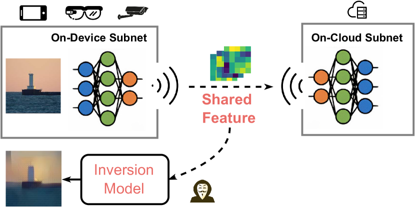
models for recovering raw data from a device (Fig. 1) therefore assume that the adversary has access to the on-device sub-network (termed as target model) as well as the shared feature activations. The adversary can be considered as either an honest-but-curious server or an eavesdropper over the communication channel. Prior attack methods Dosovitskiy and Brox (2016b); Yang et al. (2019), in addition, assume that the dataset used for training the target model (or a similar dataset Zhang et al. (2020)) are available for the adversary to train its inversion model. In practice, however, it could be unlikely for an adversary to know or obtain these real data. Moreover, a line of approaches Zhang et al. (2020); Li et al. (2022); Struppek et al. (2022) rely on pre-trained generative models Brock et al. (2019); Karras et al. (2020) to perform inversion. Due to a similar reason, it may be challenging for the adversary to obtain such generative models without having information on the real data.

In this work, we focus on a white-box and data-free model inversion attack. Previous theoretical Arora et al. (2015); Gilbert et al. (2017); Lei et al. (2019) and empirical Dosovitskiy and Brox (2016b); Teterwak et al. (2021); Hatamizadeh et al. (2022b) studies have shown that inversion attack becomes more difficult as the depth of the network that computes the feature increases. To overcome the increased complexity and non-linearity of the target model as the depth increases, we propose a divide-and-conquer inversion method that partitions the inversion into sequential layer/block-wise inversion sub-problems. For each sub-problem, an inversion module is built and optimized to reverse the input-output function of the corresponding target layer/block. To support optimization of inversion modules, we exploit synthetic data generated via minimizing the discrepancy between (randomly initialized) dummy input’s feature statistics and the corresponding statistics stored in batch normalization (BN) layer (Santos et al., 2019; Yin et al., 2020; Xu et al., 2020). With synthetic data proxies, we are able to optimize the inversion model to enforce feature embedding similarity with respect to the original counterpart. We call it cycle consistency-guided inversion. Combining aforementioned techniques enables us to successfully scale zero-shot model inversion to deep architectures and large datasets without strong assumptions on model or dataset priors.

In summary, we make the following contributions: (1) We propose an inversion method based on a divide-and-conquer inversion (DCI) and a cycle-consistency loss on synthetic data. (2) We demonstrate that the method generalizes to both discriminative and generating models, even for large datasets (i.e., ImageNet (Deng et al., 2009) and CelebA (Liu et al., 2015)), surpassing state-of-the-art baselines. (3) We demonstrate that DCI can be used as a tool to analyze the inversion difficulty at different layer depths as well as the trade-off between utility and defense.

2 Related Work

Prior model inversion attacks have been mainly pursued in three directions: analytical inversion, generative inversion, and input optimization-based inversion. This work aims to relax some strong assumptions made by prior arts, such as the requirement for real data, pretrained image priors, and intensive optimization. These assumptions may cause attacks to be time- and resource-consuming, inflexible and susceptible to distribution shifts between data used by the target model and data used for training the inversion model.

	PSiM (Dosovitskiy and Brox, 2016a, b)	IHT (Gilbert et al., 2017)	INNs (Behrmann et al., 2019, 2021)	PlugPlay (Nguyen et al., 2017; Struppek et al., 2022; Wang et al., 2021)	DI (Yin et al., 2020; Li et al., 2020c)	rMSE (He et al., 2019)	GMI (Zhang et al., 2020)	Ours
No requirement of real data	✗			✗				✓
No requirement of pretrained GAN				✗				✓
No req. of specific arch. or weights dist.		✗	✗					✓
Generalize to both disc. and gen. models	✗	✗		✗	✗		✗	✓
No adversarial training	✗			✗			✗	✓
Fast (e.g, single-pass) inversion			✗		✗	✗		✓
Sample-specific inversion				✗	✗		✗	✓

Table 1: Comparison between our approach and prior work.

Analytical Inversion. Analytical inversion studies the theoretical invertibility of neural networks Arora et al. (2014). Arora et al. (2015); Gilbert et al. (2017) theoretically show that the approximate reverse of a layer by transposing its weights matrix, based on the assumption that its weights are random-like, which is not always true for a pre-trained network Cai and Li (2019); Li et al. (2020b). Lei et al Lei et al. (2019) indicates that a layer can be inverted via linear programming assuming its output dimension is greater than twice its input dimension. However, this assumption does not hold for most classification models He et al. (2015). Despite theoretical soundness of analytical inversion, there is still a discrepancy between the setups of theories and those of contemporary pre-trained models. Moreover, these methods cannot scale to large network sizes beyond MNIST LeCun (1998)/CIFAR-10 Krizhevsky et al. (2009) level, and the recovered images are noisy (Arora et al., 2015).

Generative Inversion. Generative inversion aims to learn (or leverage) a generative model that reverses the input-output mapping of the target model. ‘Plug&Play’ methods Nguyen et al. (2017); Teterwak et al. (2021) utilize a pre-trained generator (e.g., BigGAN Brock et al. (2019)) as the ‘image prior’ to generate images that maximize the activation of the target model. If pre-trained generators are unavailable, a generative model will be trained on the original dataset of the target model Dosovitskiy and Brox (2016b); Zhang et al. (2020). The dependence on the pre-trained generator, the original dataset, and challenging adversarial learning Arjovsky et al. (2017); Kodali et al. (2017) limits the practicability of generative inversion. In addition, these methods focus on class-specific instead of accurate sample-specific inversion. For instance, given the feature of a husky dog image, generative inversion may recover a Teddy dog image because the generator adds some semantic-related (e.g, a dog in general) but sample-unrelated (i.e, the specific dog) information during inversion Zhang et al. (2020); Struppek et al. (2022). This problem would be exacerbated if the data used to train the generator had a different distribution than the original data.

Input Optimization Based Inversion. Cai et al. (2020); Haroush et al. (2020); Chawla et al. (2021) show that one can reveal certain information of training set by optimizing a dummy input to match pre-stored feature statistics (Yin et al., 2020) or maximum activation of neurons Mordvintsev et al. (2015). However, these methods are all designed to leak arbitrary training samples instead of targeted sample inversion. In addition, these methods remain computationally heavy.

Gradient Inversion. Training neural networks requires gradient estimation from a batch of data. Yin et al. (2021); Zhu et al. (2019); Li et al. (2022); Geiping et al. (2020); Hatamizadeh et al. (2022a) demonstrate that sensitive input data can be leaked given gradients. Different from gradient inversion which mainly targets on recovering input from gradients during training, we focuses on reconstructing input from feature map during inference (especially for spilt computing scenarios). More detailed comparison is provide in Tab. 3.

3 Method

Before describing the proposed method, we introduce some notations. Consider a multi-layer on-device (discriminative or generative) sub-network with $L$ layers, $\mathcal{F}_{1:L}(\mathbf{x}):=\mathcal{F}_{L}\circ\mathcal{F}_{L-1}\circ\dots\circ\mathcal{F}_{1}(\mathbf{x})$. $\mathcal{F}_{k}$ represents the $k$-th parameterized layer which may include its associated batch normalization Ioffe and Szegedy (2015) and activation. $\mathcal{F}_{k:l}$ is the sub-network containing $k$-th to $l$-th layers inclusively. In this work, we consider the following question on model inversion attacks Fredrikson et al. (2015); Wang et al. (2021): given a sub-network $\mathcal{F}_{1:L}$ pre-trained on dataset $\mathcal{D}$, is it possible to learn its approximate reverse counterpart $\mathcal{F}_{1:L}^{-1}$ (where $\mathcal{F}_{1:L}^{-1}:\mathcal{F}_{1:L}^{-1}(\mathcal{F}_{1:L}(\mathbf{x}))=\mathbf{x}^{\prime}\approx\mathbf{x}$) without access to $\mathcal{D}$?

3.1 Divide-and-Conquer Inversion

DNN consists of blocks of layers, with each layer producing an intermediate feature map that is consumed by the next layer as input. Prior research has demonstrated that neural networks produce more abstract feature maps as the depth increases Bianchini and Scarselli (2014); Eldan and Shamir (2016); Telgarsky (2016); Raghu et al. (2017). Consequently, existing studies have reported the difficulty of inverting deep models Gilbert et al. (2017); Dosovitskiy and Brox (2016b, a); Ma et al. (2018). To circumvent the difficulty of approximating all stacked layers, we first split the overall inversion problem into several layer-(or block-)wise inversion sub-problems before combining them. To this end, we present a simple yet effective inversion strategy called Divide-and-Conquer Inversion (DCI) that progressively inverts the computational flow of DNNs. Comparing to end-to-end inversions Zhang et al. (2020); Wang et al. (2021), DCI has two advantages: (1) a single layer (or block) has less non-linearity and complexity, and is therefore easier to invert; (2) DCI provides richer supervision signals across layers (or blocks), whereas the overall inversion only utilizes supervision at the two ends (i.e, the input and output) of the target model.

Starting from the first layer, DCI inverts each layer/block $\mathcal{F}_{k}$ with two goals: (i) inverting current target layer $\mathcal{F}_{k}$ with an inversion module $\mathcal{F}^{-1}_{k}$ of similar size, and (ii) fine-tuning the newly inverted module $\mathcal{F}_{k}^{-1}$ to ensure that it works well jointly with all previously inverted layers $\mathcal{F}_{1:(k-1)}^{-1}$. The necessity of the second objective comes from the non-exact inversion of each layer/block. Otherwise, a small error could be amplified along layers Dong et al. (2017). Therefore we refine inverted modules to minimize the accumulated error. According to existing literature Zhu et al. (2017); Zhang et al. (2018) We use $\ell_{1}$ distance to measure the reconstruction loss. For the first objective, we minimize the layer reconstruction loss,

$$\mathcal{L}_{\text{layer}}=\left\|\mathbf{u}_{k}-\mathcal{F}_{k}^{-1}\left(\mathcal{F}_{k}\left(\mathbf{u}_{k}\right)\right)\right\|_{1},\quad\mathbf{u}_{k}=\mathcal{F}_{1:(k-1)}(\mathbf{x}),\vspace{-1mm}$$ (1)

where $\mathbf{u}_{k}$ is the input of the target layer/block. As for the second objective, we aim to ensure the reconstruction quality of inversion modules up to the layer $k$ such that $\mathcal{F}_{1:k}^{-1}=\mathcal{F}_{k}^{-1}\circ\mathcal{F}_{1:(k-1)}^{-1}$ . This translates into minimizing the distance between inverted input $\mathbf{x}^{\prime}=\mathcal{F}_{1:k}^{-1}\left(\mathcal{F}_{1:k}\left(\mathbf{x}\right)\right)$ to the original input $\mathbf{x}$, where we introduce another loss term for this purpose:

$$\mathcal{L}_{\text{img}}(\mathbf{x},\mathbf{x}^{\prime})=\|\mathbf{x}-\mathbf{x}^{\prime}\|_{1},\quad\mathbf{x}^{\prime}=\mathcal{F}_{1:k}^{-1}\left(\mathcal{F}_{1:k}\left(\mathbf{x}\right)\right).$$ (2)

Cycle-consistency Guided Inversion. We further re-exploit the target model for stronger inversion guidance amid the unique setup of the inversion problem. As we reverse the computation of the target model, this forms a natural loop with the original computation flow. Inspired by perceptual metric Zhang et al. (2018) and cycle-consistent image translation Zhu et al. (2017), we measure the quality of reconstructed inputs by re-checking them with the target model.

The main idea is that if the reconstructed input is faithfully and semantically close to the original input then the target model should produce similar, if not exact, feature responses at all layers. To this end, we feed the reconstructed input back to the direct (target) model, and minimize the distance between features of the reconstructed input and original input at various depths. We refer to this as cycle consistency that is defined as follow:

$${\mathcal{L}_{\text{cyc}}(\mathbf{x},\mathbf{x}^{\prime})=\Sigma_{l=1}^{L}\|\mathcal{F}_{1:l}(\mathbf{x})-\mathcal{F}_{1:l}(\mathbf{x}^{\prime})\|_{1}}.\vspace{-1mm}$$ (3)

This enables a better utilization of the features from the original input twice to provide richer supervision: (i) In Eq. 1, we use features of the original input $\mathcal{F}_{1:(k-1)}(\mathbf{x})$ as the reconstruction objective; (ii) The cycle consistency loss (Eq. 3) also uses features of the original input as a reference and enforces the inverted input similar to those of the original input.

With all the above losses, the overall optimization objective for an inversion layer can thus be expressed as $\mathcal{L}_{k}=\mathcal{L}_{\text{layer}}+\mathcal{L}_{\text{img}}+\mathcal{L}_{\text{cyc}}$.

3.2 Data Sampling

One remaining challenge to optimize inversion modules is how to obtain input data $\mathbf{x}$. When the target model is a generative model (i.e., the generator of a generative adversarial network Aggarwal et al. (2021)), obtaining input data is as simple as randomly sampling latent codes from a Normal distribution Arjovsky et al. (2017). However, when the target model is a discriminative model, it is infeasible to sample data from the original data distribution under the data-free setting.

Inspired by adversarial-free generative models Li et al. (2017); Bińkowski et al. (2018) and data-free knowledge distillation Yin et al. (2020); Xu et al. (2020), we leverage these techniques to generate a small dataset for training of inversion modules. In particular, we generate a batch of data by minimizing the difference between features statistics of the synthetic data $\hat{\mathbf{x}}$ and statistics stored in batch normalization (BN):

$${\text{min}}_{\hat{\mathbf{x}}}{\ \sum\nolimits_{l}||\mu_{l}(\mathbf{\hat{x}})-\text{BN}_{l}(\mu)||_{2}+\sum\nolimits_{l}||{\sigma^{2}_{l}}(\mathbf{\hat{x}})-\text{BN}_{l}(\sigma^{2})||_{2}}+\lambda\mathcal{R}_{\text{img}}(\hat{\mathbf{x}}).\vspace{-1mm}$$ (4)

Here, $\mu_{l}(\hat{\mathbf{x}})$ and $\sigma^{2}_{l}(\hat{\mathbf{x}})$ are features statistics computed at the $l$-th layer. $\text{BN}_{l}(\mu)$ and $\text{BN}_{l}(\sigma^{2})$ are their corresponding statistics stored in a BN layer. $\mathcal{R}_{\text{img}}$ is the image regularization like total variance Guo et al. (2017) to make derived images more natural Yin et al. (2020). Minimizing the difference of features’ statistics is equivalent to reducing the probability distance Li et al. (2017) between distributions of synthetic data and real data Choi et al. (2020). Thus, the synthetic data can be treated as data from a distribution that is similar to the underlying distribution of real data and thus can serve as a reasonable proxy for training of our inversion modules.

Note that there is still a gap between the synthetic and original real data. Different from our approach, prior generative inversions cannot utilize this synthetic data because they are sensitive to this gap due to the following reasons: (1) Generative inversions Dosovitskiy and Brox (2016b); Teterwak et al. (2021) train a generator (in a GAN framework) as the inversion model, whereas the GAN training is very sensitive and challenging given only synthetic data Kodali et al. (2017); Tran et al. (2021); Zhao et al. (2020). The resulting efficacy falls short to DCI, as we will show later in Sec. 4.2. (2) Prior works Nguyen et al. (2017); Dosovitskiy and Brox (2016b); Teterwak et al. (2021) require the whole training set (e.g., more than $1$M images) to train the GAN. Yet deriving massive synthetic data remains slow Yin et al. (2020). In contrast, without any adversarial learning, DCI does not have the above disadvantages when using synthetic data because of its progressive inversion nature and cycle consistency supervision. DCI is data-efficient and can be enabled by only $10$K synthetic images. In contrast, generative methods requires the access to the original ImageNet training dataset containing 1.28M real images Zhang et al. (2020); Nguyen et al. (2017).

4 Evaluation

In this section, we demonstrate the efficacy of our inversion attack to discriminative and generative models. Without any strong assumptions such as real data, costly input optimization, or pre-trained image priors, we significantly scale model inversion attack to very deep architectures (e.g., RepVGG-A0, ResNet-18, ResNet-50, and SNGAN), high resolution input (e.g., $224\times 224$px for ImageNet and $128\times 128$px for CelebA), and different pre-training methods for the target model (e.g., supervised and self-supervised). Due to page limit, we present more implementation details (Appendix B), additional inversion results (Appendix C), and ablation studies (Appendix D) in the appendix.

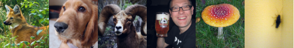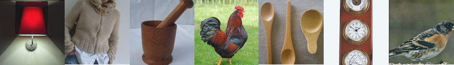
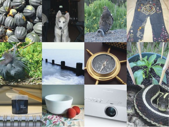
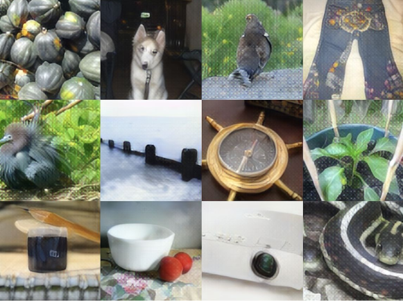
Real images $\mathbf{x}$ from the ImageNet validation set.

Inverted images from ResNet-50’s (supervised He et al. (2015)) features after $42$ conv. layers.

Inverted images from ResNet-50’s (MoCoV2 (Chen et al., 2020b)) features after $42$ conv. layers.

Figure 2: Inversion attacks to ResNet-50 (sup. and self-sup.) without access to any real data.

4.1 Inversion Attack to Deep Models on the ImageNet Dataset

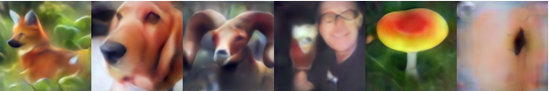
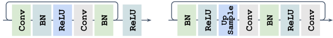
Inversion Attack to RepVGG-A0. We consider the inversion of RepVGG Ding et al. (2021), which is one of the state-of-the-art classification models with a deep architecture. It has a ResNet-like He et al. (2015) multi-branch topology during training, and a mathematically equivalent VGG-like Simonyan and Zisserman (2014) inference-time architecture, which is achieved by layer folding. Specifically, we consider RepVGG-A0 Ding et al. (2021) with $22$ convolution blocks, each of which is comprised of a convolution, ReLU, and BN layer, yielding a $72.41\%$ top-1 accuracy on ImageNet Ding et al. (2021). Using our DCI strategy, We invert one block with an inversion module at a time. Each inversion module has a similar architecture as its target counterpart but with reversed input-output dimensions, and is optimized via Adam Kingma and Ba (2014) for $6$K iterations. We use $10$K synthetic images as detailed in Sec. 3.2 to train inversion modules. Inversion attack results are displayed in Fig. 3. Remarkably, our inversion recovers very close pixel-wise proxy to the original image from the $21$-th layer’s activation (with spatial size $14\times 14$), preserving original semantic and visual attributes, such as color, orientation, outline, and position.

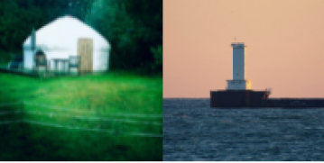
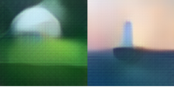
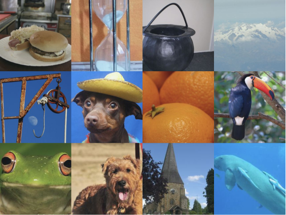
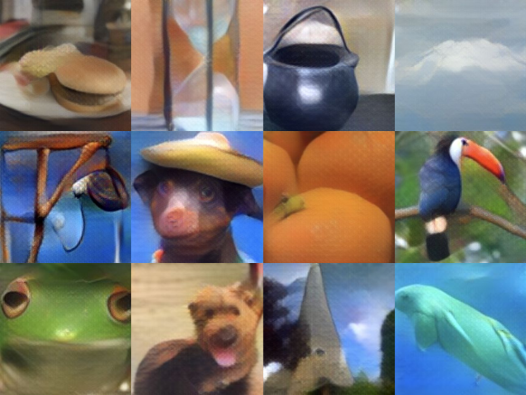
Real images $\mathbf{x}$ of $224\times 224$ px. from the ImageNet validation set.

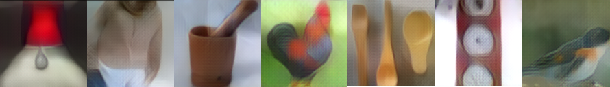Recovered images from features after 21 blocks $\mathcal{F}_{1:21}^{-1}(\mathcal{F}_{1:21}(\mathbf{x})\big{)}$ .

Figure 3: Inversion Attack to a pre-trained RepVGG.

Inversion Attack at Varying Depths. We visualize the inverted images from different layer depths of the target model in Fig. 4. As the depth increases, inverted images become more blurry, losing mo-

Figure 4: Inversion from features at increased depths. (Left) Number indicates layer depth. (Right) PSNR and LPIPS at various layer depths. Shaded region is the standard deviation across samples from ImageNet validation set.

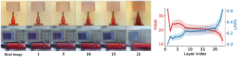
re details. It is caused by information filtering due to the classification nature of the model Yosinski et al. (2014). To quantify the changes, we also provide peak signal-to-noise ratio (PSNR) psn (2021) and perceptual metric (LPIPS) Zhang et al. (2018) between real and inverted images at different depths. The quantitative results are consistent with the qualitative observations. An intriguing observation from Fig. 4 is the consistent preservation of high level information across the majority of layers, which challenges prior security arguments in split computing Kang et al. (2017); Eshratifar et al. (2019); Dong et al. (2022). As shown in Fig. 4, we can achieve nearly perfect recovery from outputs of the $5$-th blocks (with spatial size $28\times 28$) that already past three stride-$2$ convolutions. which were regarded as lossy operations. We find that increasing the depth of on-device sub-network is not always effective in making inversion more difficult. For example, in Fig. 4 (right), features from the $8$-th to $16$-th blocks results in inverted images with comparable quality in terms of PSNR and LPIPS. In addition, we notice an obvious drop of inversion quality (i.e, PSNR) after the second convolution layer which has 48 in and out channels with a stride of 2. This layer repeatedly reduces the feature size from $48\cdot 112^{2}$ to $48\cdot 56^{2}$, resulting in information loss Ma et al. (2019); Zhu and Blaschko (2020) and increased inversion difficulty. The following (i.e, the third) layer has a stride of 1 and the same input and output sizes. According to Fig. 4 (right), this layer may enhance some information Hermann and Lampinen (2020), resulting in an improved inversion quality.

In addition, we find that the final two layers dramatically degrade the inversion quality. One can still recognize the class of inverted images after the penultimate (i.e., the $22$-nd convolution) block. However, if we invert features after the final (i.e., the fully-connected) layer, only the predominant color is discernible as shown in Appendix C. This suggests that class-invariant information is rapidly filtered out towards the end of the model. This is consistent with observations in transfer learning Yosinski et al. (2014); Li et al. (2020a); Zoph et al. (2020) and self-supervised learning He et al. (2020a); Grill et al. (2020); Chen et al. (2020a).

These results provides several insights to the privacy vulnerability of split computing. For an extremely compact edge device, only few (e.g., 5) blocks can be on the device and the other layers have to be on the cloud. In this case, inverting from the output of the 5-th blocks results in recovered images with many details, e.g., in Fig. 4, even tiny bottoms and knobs on the oscilloscope are well recognizable. If the edge device has mediate computation/memory capacity, more (e.g., 15) layers can be on the device. Inverting from 15-th block’s output will mainly reveal “large structures” (e.g., outlines, colors, and shapes), also leading to privacy concerns. Both cases debunk privacy of split computing that is presumed safe.

Inversion Attack to ResNets. To demonstrate the general applicability of the proposed method, we present inversion results for additional networks on the ImageNet dataset, encompassing a variety of architectures (ResNet-$18$ and ResNet-$50$) and pre-training methods (standard He et al. (2015) and self-supervised Chen et al. (2020b)). Each BasicBlock unit in ResNet-18 comprises

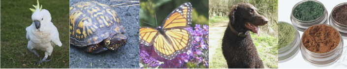
Real images from the ImageNet validation set.

Inverted images after $15$ conv. layers $\mathcal{F}_{1:15}^{-1}(\mathcal{F}_{1:15}(\mathbf{x})\big{)}$ .

Figure 5:   Inversion attack to a pre-trained ResNet-18.

two convolution layers (with BN and ReLU) and a shortcut connection, and is inverted individually. Fig. 5 depicts the inversion results of pre-trained ResNet-$18$ on ImageNet. With the proposed method, we can recover recognizable input images after up to $7$ blocks that contain a total of $15$ convolution layers and one maxpooling layer. We observe inversion can still restore images with high fidelity that contain similar visual details as the original images.

We next move to invert pre-trained ResNet-$50$ and investigate both a standard supervised model He et al. (2015), and the recent self-supervised model MoCoV2 Chen et al. (2020b) in Fig. 2. We observe that a stronger feature extractor (i.e., MoCoV2) preserves more information, resulting stronger inversion, when compared to a standard supervised training of the same network architecture (the second and third rows in Fig. 2). This is consistent with the recent findings in Yin et al. (2021), showing that self-supervised models are more vulnerable to gradient inversion attack. These results demonstrate that we are able to recover recognizable input images for up to $42$ convolution layers and one max pooling layer in total.

4.2 Comparison to Prior Art on Inversion Attack

We compare DCI to prior model inversion attacks under the data-free setting in Fig. 8 and Tab. 2. Among the baselines considered, DDream Mordvintsev et al. (2015) and DI Yin et al. (2020) are data-free approaches. They randomly initialize a dummy input and optimize it to recover data samples. Since these methods start from random initialization, it is unlikely to recover a specific instance of input image. Moreover, most of inverted images are visually bizarre. DCI utilizes the synthetic data generated by DI Yin et al. (2020) to optimize inversion modules, and achieves sample-level inversion with significantly improved quality of inverted images. In addition, both DDream and DI require 20K forward and backward passes to optimize inputs – while our method only needs one forward pass through inversion modules, hence is more efficient. PSiM Dosovitskiy and Brox (2016b) and GMI Zhang et al. (2020) require the original training data of the target model and auxiliary data Zhang et al. (2020) to train the inversion model. For a fair comparison, their inversion models are instead trained using synthetic data. As we discussed in Sec. 3.2, these generative inversions do not work well under data-free setting due to their sensitivity to shifts between real and synthetic data distributions.

4.3 Inversion Attack to GAN on the CelebA Dataset

We next demonstrate that our DCI can also be applied to generative models. This experiment focuses on the popular SNGAN architecture that has $2.72$ Inception Score (IS) on the CelebA dataset of $128\times 128$px resolution Miyato et al. (2018). SNGAN Miyato et al. (2018) comprises $17$ layers, including one fully-connected layer at the start, one convolution layer at the end, and $5$ residual blocks. Each residual block consists of $3$ convolution layers kwotsin (2021).

We partition the inversion of the entire SNGAN model into inversions of the first fully-connected layer, the last convolution layer, and each of $5$ residual blocks. For mathematical consistency with prior GAN literature, we use $\mathcal{G}:\mathbf{z}\rightarrow\mathbf{x}$ to indicate the target generator. $\mathbf{z}$ represents the real latent code that generates $\mathbf{x}=\mathcal{G}(\mathbf{z})$. We aim to learn $\mathcal{G}^{-1}$ that faithfully reconstructs $\mathbf{z}$ given $\mathbf{x}$. To evaluate the quality of inversion, we use the inverted latent code $\mathbf{z}^{\prime}$ to re-generate an image $\mathbf{x}^{\prime}=\mathcal{G}(\mathbf{z}^{\prime})$, which is referred to as the second generation.

The adversary can manipulate the second generation by varying the inverted latent code for downstream attacks Xia et al. (2022).

Figure 6: Images from interpolation of inverted latent codes

$\mathcal{G}(\alpha\cdot\mathbf{z}^{\prime}_{1}+(1-\alpha)\cdot\mathbf{z}^{\prime}_{2})$

.

For instance, an adversary may perform linear interpolation between inverted latent codes $\alpha\cdot\mathbf{z^{\prime}_{1}}+(1-\alpha)\cdot\mathbf{z^{\prime}_{2}}$ with different factor $\alpha\in\{0,0.2,0.4,0.6,0.8,1.0\}$ in Fig. 6 to get manipulated images. In addition, results of Fig. 6 validate that the inverted latent codes fit into the original latent code distribution, akin to GAN inversion literature Lei et al. (2019); Xia et al. (2022).

SNGAN generated samples $\mathbf{x}=\mathcal{G}(\mathbf{z})$ .

Inverted images $\mathbf{x}^{\prime}=\mathcal{G}(\mathcal{G}^{-1}(\mathcal{G}(\mathbf{z})))$ .

Figure 7: Inversion attack to SNGAN.

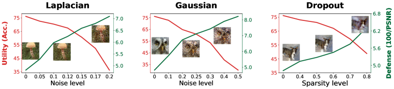
4.4 Trade-off between Utility and Defense

We next demonstrate that it is quite challenging to defend against the proposed inversion attack by perturbing features while preserving the accuracy of target model. Following prior work of split computing Teerapittayanon et al. (2017); Verbraeken et al. (2020); Dong et al. (2022), we use the first $35$ layers of ResNet-50 as the on-device sub-network and perform inversion attack to the features generated by this sub-network. Three widely used defense strategies are tested as follows.

Noise Injection. One straightforward attempt to defend inversion attack is to add noise on features before sharing Pettai and Laud (2015). We experiment with Gaussian and Laplacian noises which are widely used in defenses of inversion attacks  Vepakomma et al. (2018); Titcombe et al. (2021) and differential privacy studies Abadi et al. (2016); Zhu et al. (2020); Gawron and Stubbings (2022). We refer to the standard deviation of a noise distribution as noise level and increase it gradually to observe the trade-off between utility and defense, which are measured by the accuracy of the target model and $\frac{100}{\text{PSNR}}$, respectively. A greater $\frac{100}{\text{PSNR}}$ value indicates increased resistance to inversion attack. we observe that the trade-off between utility and defense mainly depends on the magnitude of noise levels and less related to the noise types. In addition, both types of noises will introduce a non-negligible accuracy drop for the target model. For instance, after adding Laplacian noise with the scale of $0.2$, the recovered images are still clearly recognizable. However, the accuracy of target model drops for about $20\%$ because of the noise.

Feature Dropout. We also experiment feature dropout defense by randomly setting elements in features to zero He et al. (2020b). The results of varying the sparsity level of features are shown in Fig. 9. We observe that all defense methods will degrade the target model’s accuracy and impede the inversion attack simultaneously. Although feature dropout can better preserve target model’s accuracy, it also has less defense effect. These findings validate the non-trivial trade-off between utility and defense, and motivates future research on advanced defense.

Real	PSiM Dosovitskiy and Brox (2016b)	GMI Zhang et al. (2020)	DDream Mordvintsev et al. (2015)	DI Yin et al. (2020)	rMSE He et al. (2019)	Ours

Figure 8: Qualitative comparison on RepVGG-A0 inversion under data-free setting.

Method	PSiM Dosovitskiy and Brox (2016b)	GMI Zhang et al. (2020)	rMSE He et al. (2019)	DDream Mordvintsev et al. (2015)	DI Yin et al. (2020)	Ours
MSE $\downarrow$	$0.092$	$0.104$	$0.082$	$0.186$	0.080	$\mathbf{0.013}$
LPIPS $\downarrow$	$0.725$	$0.751$	$1.082$	$0.904$	$0.602$	$\mathbf{0.443}$
PSNR $\uparrow$	$9.080$	$9.395$	$10.90$	$9.534$	$10.93$	$\mathbf{18.83}$
Inference† (s) $\downarrow$	$2.4\times 10^{-1}$	$7.2\times 10^{-2}$	$2.1\times 10^{2}$	$5.5\times 10^{2}$	$1.9\times 10^{3}$	$\bm{1.5\times 10^{-2}}$
† Inference time measured on NVIDIA V100 GPU for one inversion of batch size $4$.

Table 2: Quantitative comparison to prior methods under the data-free setting.

Figure 9: The utility and defense trade-off of defense strategies. Red (green) lines are the accuracy (defense effect $\frac{100}{\text{PSNR}}$) when different noise/sparsity levels are applied to features.

5 Conclusion

This work presents Divide-and-Conquer Inversion (DCI) that scales model inversion attack to large-scale datasets (e.g, ImageNet and CelebA), deep architectures (e.g, RepVGG and ResNet), and different model types (e.g, discriminative and generative). Our experimental results show that it is still possible to recover well recognizable images given features after up 42 convolutional layers on ImageNet while existing attacks all fail. We hope the proposed method can serve as a tool for empirically measuring the amount of data leakage and facilitate the future study on privacy of split computing.

Appendix A Additional Related Work

Autoencoder. Model inversion is also related to autoencoders Vincent et al. (2010); Hinton et al. (2011) given a similar functionality of target and inversion models, to an encoder-decoder pair. However, the encoder and decoder in an autoencoder are trained jointly with a vast amount of data in an end-to-end manner. In our case, only an individually pre-trained target model is accessible. Aligning with the previous finding of layer-wise training of autoencoder (e.g., deep belief network Hinton et al. (2006); Bengio et al. (2007)), we also find layer-wise training beneficial for inversion model training as detailed in Sec. 3.1.

Invertible Neural Networks. Invertible neural networks (INNs) Behrmann et al. (2021); Dinh et al. (2016); Kingma and Dhariwal (2018) are a family of neural networks which is theoretically invertible due to their special architectures and weights. For instance, i-RevNet Jacobsen et al. (2018) uses carefully planned convolution, reshuffling, and partitioning procedures to ensure inversion. i-ResNet Behrmann et al. (2019) constrains weights with Lipschitz condition. In conclusion, INNs are inapplicable to standard model architectures since they depend on uncommon architectures and regularizations.

Table 3: Key differences between Gradient Inversion and Feature Inversion (Ours)

	Gradient Inversion Yin et al. (2021); Zhu et al. (2019); Li et al. (2022); Geiping et al. (2020); Hatamizadeh et al. (2022a)	Feature Inversion (Ours)
Scenario	Federated learning (training)	Split computing (inference)
Input	Weights + Gradients	Weights + Features
Goal	Exact image recovery from gradients	Exact image recovery from features
Insight	Gradients encode private information via inversion	Features encode private information via even faster inversion

Appendix B Implementation Details

B.1 Training Strategy

DCI divides the computation of a feed-forward neural network into multiple parts and inverts the computational flow progressively. One straightforward strategy is to sequentially optimize each individual inversion module $\mathcal{F}_{k}^{-1}$, beginning with the first layer $\mathcal{F}_{1}^{-1}$. We observe that as we progress deeper into the model, the inversion error will increase. To address this accumulation issue, we use a more potent training strategy. After optimizing a particular inversion module $\mathcal{F}_{k}^{-1}$, we take into account all previous inversion modules and fine-tune all layers up to $k$, i.e., $\mathcal{F}_{1}^{-1}\circ\dots\circ\mathcal{F}_{k-1}^{-1}\circ\mathcal{F}_{k}^{-1}$, with the same loss $\mathcal{L}_{k}$ to reduce the accumulated inversion error. When $k=1$, this fine-tuning is skipped because there is no inversion model prior to $\mathcal{F}_{1}^{-1}$.

B.2 Inversion Models

ResNet-18. The first four sequential layers in ResNet models are convolution, BN, ReLU, and max pooling layers, and we invert the sequence of the first four layers as a whole block. Each inversion module mimics the architecture of its corresponding target counterpart but with reversed input and output dimensions. For a BasicBlock (left) in ResNet-18, its inversion module (right) is shown as below in Fig. 10.

Figure 10: (Left) A BasicBlock in ResNet-18 (Right) Corresponding inversion module for the BasicaBlock.

ResNet-50. We break the overall ResNet-$50$ architecture into five sub-networks and invert one sub-network each time. Similar to ResNet-$18$, the first sub-network is the initial block. The other four sub-networks consist of $3,4,6,3$ repeats of Bottleneck respectively He et al. (2015).

Appendix C Additional Inversion Results

Lossy Final Fully-Connected Layer. In the main manuscript, we show that the recovered images from RepVGG feature embeddings after $21$ convolution layers preserve original semantic and visual attributes. However, we find that information in the feature embeddings decays rapidly through the last two layers in RepVGG. This may indicate that class-invariant information is quickly filtered out towards the end of the model while the initial stages focus on feature extraction, which is aligned with prior observations in transfer learning Yosinski et al. (2014); Li et al. (2020a); Long et al. (2015); Dollár (2018); Zoph et al. (2020) and self-supervised learning He et al. (2020a); Grill et al. (2020); Chen et al. (2020a). We visualize the above findings in Fig. 11. One can still recognize the class of inverted images after the penultimate (i.e., the $22$-th convolution) layer. However, if we invert features after the final (i.e., the fully-connected) layer, only the predominant color is recognizable.

(a) Original images	(b) Inversion from the last convolution layer	(c) Inversion from the final full-connected layer

Figure 11: Results of inversion from (b) the penultimate layer (i.e., the last convolution layer), and (c) the final layer (i.e., the final full-connected layer)

Appendix D Ablation Studies

Effectiveness of Synthetic Data.

Real images $\mathbf{x}$ from the ImageNet validation set.

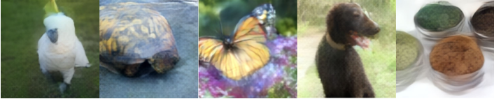Inverted images by inversion model trained on 1K real data.   (LPIPS $\downarrow$ = 0.462)

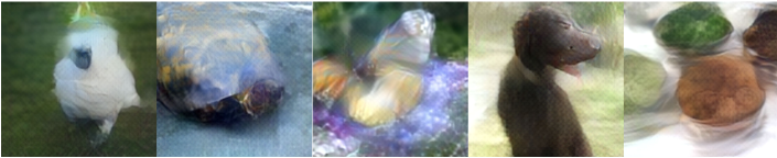Inverted images by inversion model trained on 1K synthetic data.   (LPIPS $\downarrow$ = 0.481)

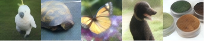Inverted images by inversion model trained on 10K real data.    (LPIPS $\downarrow$ = 0.430)

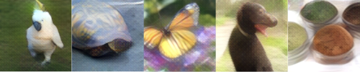Inverted images by inversion model trained on 10K synthetic data. (LPIPS $\downarrow$ = 0.443)

Figure 12: Comparison of different data settings. Our method achieves a comparable inversion quality using synthetic data compared to using real data.

We study how well synthetic data may be used to optimize our inversion modules. For a sanity check, we re-perform the experiment in Fig. 3 using real data from ImageNet training set rather than the synthetic data. We also vary the number of synthetic data used for optimization. In Fig. 12, we show that using more (real or synthetic) data samples improves the inversion quality. For instance, in the first column of Fig. 12, the inverted images can reveal the parrot’s tiny eyes when 10K (real or synthetic) images are used for the optimization of inversion modules. However, we also discover that when there are more than 10K (real or synthetic) samples, the improvement of inversion quality is limited. In addition, we demonstrate that DCI achieves a comparable inversion quality when using synthetic data as opposed to using real data. However, due to their sensitivity to data distribution change, as illustrated in Fig. 8, prior generative inversion approaches Nguyen et al. (2017); Zhang et al. (2020) cannot efficiently use synthetic data.

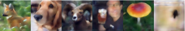
Real images $\mathbf{x}$ from the ImageNet validation set.

Inverted images from ResNet-50’s (supervised) features after 35 conv. layers.

Figure 13: More inversion results on ResNet-50 without any real data. Our method generalizes well on different types of images.

Real images $\mathbf{x}$ from the ImageNet validation set.

Inverted images from RepVGG-A0 features after 21 conv. layers.

Figure 14: More inversion results on RepVGG-A0 without any real data. Our method generalizes well on different types of images.

References

- psn (2021) Peak signal-to-noise ratio. https://en.wikipedia.org/wiki/Peak_signal-to-noise_ratio, 2021.
- Abadi et al. (2016) Martin Abadi, Andy Chu, Ian Goodfellow, H Brendan McMahan, Ilya Mironov, Kunal Talwar, and Li Zhang. Deep learning with differential privacy. In Proceedings of the 2016 ACM SIGSAC conference on computer and communications security, pages 308–318, 2016.
- Aggarwal et al. (2021) Alankrita Aggarwal, Mamta Mittal, and Gopi Battineni. Generative adversarial network: An overview of theory and applications. International Journal of Information Management Data Insights, 1(1):100004, 2021.
- Arjovsky et al. (2017) Martin Arjovsky, Soumith Chintala, and Léon Bottou. Wasserstein generative adversarial networks. In International conference on machine learning, pages 214–223. PMLR, 2017.
- Arora et al. (2014) Sanjeev Arora, Aditya Bhaskara, Rong Ge, and Tengyu Ma. Provable bounds for learning some deep representations. In International conference on machine learning, pages 584–592. PMLR, 2014.
- Arora et al. (2015) Sanjeev Arora, Yingyu Liang, and Tengyu Ma. Why are deep nets reversible: A simple theory, with implications for training. In ICLR, 2015.
- Behrmann et al. (2019) Jens Behrmann, Will Grathwohl, Ricky TQ Chen, David Duvenaud, and Jörn-Henrik Jacobsen. Invertible residual networks. In International Conference on Machine Learning, pages 573–582. PMLR, 2019.
- Behrmann et al. (2021) Jens Behrmann, Paul Vicol, Kuan-Chieh Wang, Roger Grosse, and Jörn-Henrik Jacobsen. Understanding and mitigating exploding inverses in invertible neural networks. In International Conference on Artificial Intelligence and Statistics, pages 1792–1800. PMLR, 2021.
- Bengio et al. (2007) Yoshua Bengio, Pascal Lamblin, Dan Popovici, Hugo Larochelle, et al. Greedy layer-wise training of deep networks. Advances in neural information processing systems, 19:153, 2007.
- Bianchini and Scarselli (2014) Monica Bianchini and Franco Scarselli. On the complexity of neural network classifiers: A comparison between shallow and deep architectures. IEEE transactions on neural networks and learning systems, 25(8):1553–1565, 2014.
- Bińkowski et al. (2018) Mikołaj Bińkowski, Dougal J Sutherland, Michael Arbel, and Arthur Gretton. Demystifying mmd gans. ICLR, 2018.
- Brock et al. (2019) Andrew Brock, Jeff Donahue, and Karen Simonyan. Large scale GAN training for high fidelity natural image synthesis. In International Conference on Learning Representations, 2019. URL https://openreview.net/forum?id=B1xsqj09Fm.
- Cai and Li (2019) Wen-Pu Cai and W. Li. Weight normalization based quantization for deep neural network compression. ArXiv, abs/1907.00593, 2019.
- Cai et al. (2020) Yaohui Cai, Zhewei Yao, Zhen Dong, Amir Gholami, Michael W Mahoney, and Kurt Keutzer. ZeroQ: A novel zero shot quantization framework. In Proc. CVPR, 2020.
- Chawla et al. (2021) Akshay Chawla, Hongxu Yin, Pavlo Molchanov, and Jose Alvarez. Data-free knowledge distillation for object detection. In Proceedings of the IEEE/CVF Winter Conference on Applications of Computer Vision, pages 3289–3298, 2021.
- Chen et al. (2020a) Ting Chen, Simon Kornblith, Kevin Swersky, Mohammad Norouzi, and Geoffrey Hinton. Big self-supervised models are strong semi-supervised learners. NeurIPS, 2020a.
- Chen et al. (2020b) Xinlei Chen, Haoqi Fan, Ross Girshick, and Kaiming He. Improved baselines with momentum contrastive learning. arXiv preprint arXiv:2003.04297, 2020b.
- Choi et al. (2020) Yoojin Choi, Jihwan Choi, Mostafa El-Khamy, and Jungwon Lee. Data-free network quantization with adversarial knowledge distillation. In Proceedings of the IEEE/CVF Conference on Computer Vision and Pattern Recognition Workshops, pages 710–711, 2020.
- Deng et al. (2009) Jia Deng, Wei Dong, Richard Socher, Li-Jia Li, Kai Li, and Li Fei-Fei. Imagenet: A large-scale hierarchical image database. In 2009 IEEE conference on computer vision and pattern recognition, pages 248–255. Ieee, 2009.
- Ding et al. (2021) Xiaohan Ding, Xiangyu Zhang, Ningning Ma, Jungong Han, Guiguang Ding, and Jian Sun. Repvgg: Making vgg-style convnets great again. CVPR, 2021.
- Dinh et al. (2016) Laurent Dinh, Jascha Sohl-Dickstein, and Samy Bengio. Density estimation using real nvp. arXiv preprint arXiv:1605.08803, 2016.
- Dollár (2018) Kaiming He Ross Girshick Piotr Dollár. Rethinking imagenet pre-training. 2018.
- Dong et al. (2017) Xin Dong, Shangyu Chen, and Sinno Pan. Learning to prune deep neural networks via layer-wise optimal brain surgeon. Advances in Neural Information Processing Systems, 30, 2017.
- Dong et al. (2022) Xin Dong, Barbara De Salvo, Meng Li, Chiao Liu, Zhongnan Qu, HT Kung, and Ziyun Li. Splitnets: Designing neural architectures for efficient distributed computing on head-mounted systems. In Proceedings of the IEEE/CVF Conference on Computer Vision and Pattern Recognition, pages 12559–12569, 2022.
- Dosovitskiy and Brox (2016a) Alexey Dosovitskiy and Thomas Brox. Inverting visual representations with convolutional networks. In IEEE/CVF Conference on Computer Vision and Pattern Recognition, 2016a.
- Dosovitskiy and Brox (2016b) Alexey Dosovitskiy and Thomas Brox. Generating images with perceptual similarity metrics based on deep networks. Advances in Neural Information Processing Systems, 2016b.
- Eldan and Shamir (2016) Ronen Eldan and Ohad Shamir. The power of depth for feedforward neural networks. In Conference on learning theory, pages 907–940. PMLR, 2016.
- Eshratifar et al. (2019) Amir Erfan Eshratifar, Amirhossein Esmaili, and Massoud Pedram. Bottlenet: A deep learning architecture for intelligent mobile cloud computing services. In 2019 IEEE/ACM International Symposium on Low Power Electronics and Design (ISLPED), pages 1–6. IEEE, 2019.
- Fredrikson et al. (2015) Matt Fredrikson, Somesh Jha, and Thomas Ristenpart. Model inversion attacks that exploit confidence information and basic countermeasures. In Proceedings of the 22nd ACM SIGSAC conference on computer and communications security, pages 1322–1333, 2015.
- Gawron and Stubbings (2022) Grzegorz Gawron and Philip Stubbings. Feature space hijacking attacks against differentially private split learning. arXiv preprint arXiv:2201.04018, 2022.
- Geiping et al. (2020) Jonas Geiping, Hartmut Bauermeister, Hannah Dröge, and Michael Moeller. Inverting gradients-how easy is it to break privacy in federated learning? Advances in Neural Information Processing Systems, 33:16937–16947, 2020.
- Gilbert et al. (2017) Anna C. Gilbert, Yi Zhang, Kibok Lee, Yuting Zhang, and Honglak Lee. Towards understanding the invertibility of convolutional neural networks. In IJCAI, 2017.
- Grill et al. (2020) Jean-Bastien Grill, Florian Strub, Florent Altché, Corentin Tallec, Pierre H Richemond, Elena Buchatskaya, Carl Doersch, Bernardo Avila Pires, Zhaohan Daniel Guo, Mohammad Gheshlaghi Azar, et al. Bootstrap your own latent: A new approach to self-supervised learning. arXiv preprint arXiv:2006.07733, 2020.
- Guo et al. (2017) Chuan Guo, Mayank Rana, Moustapha Cisse, and Laurens Van Der Maaten. Countering adversarial images using input transformations. arXiv preprint arXiv:1711.00117, 2017.
- Haroush et al. (2020) Matan Haroush, Itay Hubara, Elad Hoffer, and Daniel Soudry. The knowledge within: Methods for data-free model compression. In Proc. CVPR, 2020.
- Hatamizadeh et al. (2022a) Ali Hatamizadeh, Hongxu Yin, Holger R Roth, Wenqi Li, Jan Kautz, Daguang Xu, and Pavlo Molchanov. Gradvit: Gradient inversion of vision transformers. In Proceedings of the IEEE/CVF Conference on Computer Vision and Pattern Recognition, pages 10021–10030, 2022a.
- Hatamizadeh et al. (2022b) Ali Hatamizadeh, Hongxu Yin, Holger R. Roth, Wenqi Li, Jan Kautz, Daguang Xu, and Pavlo Molchanov. GradViT: Gradient inversion of vision transformers. In Proceedings of the IEEE/CVF Conference on Computer Vision and Pattern Recognition (CVPR), pages 10021–10030, June 2022b.
- He et al. (2015) Kaiming He, Xiangyu Zhang, Shaoqing Ren, and Jian Sun. Deep residual learning for image recognition. arXiv preprint arXiv:1512.03385, 2015.
- He et al. (2020a) Kaiming He, Haoqi Fan, Yuxin Wu, Saining Xie, and Ross Girshick. Momentum contrast for unsupervised visual representation learning. In Proceedings of the IEEE/CVF Conference on Computer Vision and Pattern Recognition, pages 9729–9738, 2020a.
- He et al. (2019) Zecheng He, Tianwei Zhang, and Ruby B Lee. Model inversion attacks against collaborative inference. In Proceedings of the 35th Annual Computer Security Applications Conference, pages 148–162, 2019.
- He et al. (2020b) Zecheng He, Tianwei Zhang, and Ruby B Lee. Attacking and protecting data privacy in edge–cloud collaborative inference systems. IEEE Internet of Things Journal, 8(12):9706–9716, 2020b.
- Hermann and Lampinen (2020) Katherine Hermann and Andrew Lampinen. What shapes feature representations? exploring datasets, architectures, and training. Advances in Neural Information Processing Systems, 33:9995–10006, 2020.
- Hinton et al. (2006) Geoffrey E Hinton, Simon Osindero, and Yee-Whye Teh. A fast learning algorithm for deep belief nets. Neural computation, 18(7):1527–1554, 2006.
- Hinton et al. (2011) Geoffrey E Hinton, Alex Krizhevsky, and Sida D Wang. Transforming auto-encoders. In International conference on artificial neural networks, pages 44–51. Springer, 2011.
- Ioffe and Szegedy (2015) Sergey Ioffe and Christian Szegedy. Batch normalization: Accelerating deep network training by reducing internal covariate shift. In International conference on machine learning, pages 448–456. PMLR, 2015.
- Jacobsen et al. (2018) Jörn-Henrik Jacobsen, Arnold Smeulders, and Edouard Oyallon. i-revnet: Deep invertible networks. ICLR, 2018.
- Kang et al. (2017) Yiping Kang, Johann Hauswald, Cao Gao, Austin Rovinski, Trevor Mudge, Jason Mars, and Lingjia Tang. Neurosurgeon. In Proceedings of the Twenty-Second International Conference on Architectural Support for Programming Languages and Operating Systems. ACM, 2017. 10.1145/3037697.3037698. URL http://dl.acm.org/ft_gateway.cfm?id=3037698&type=pdf.
- Karras et al. (2020) Tero Karras, Samuli Laine, Miika Aittala, Janne Hellsten, Jaakko Lehtinen, and Timo Aila. Analyzing and improving the image quality of stylegan. In Proceedings of the IEEE/CVF conference on computer vision and pattern recognition, pages 8110–8119, 2020.
- Kingma and Ba (2014) Diederik P Kingma and Jimmy Ba. Adam: A method for stochastic optimization. ICLR, 2014.
- Kingma and Dhariwal (2018) Diederik P Kingma and Prafulla Dhariwal. Glow: Generative flow with invertible 1x1 convolutions. arXiv preprint arXiv:1807.03039, 2018.
- Kodali et al. (2017) Naveen Kodali, Jacob Abernethy, James Hays, and Zsolt Kira. On convergence and stability of gans. arXiv preprint arXiv:1705.07215, 2017.
- Krizhevsky et al. (2009) Alex Krizhevsky, Geoffrey Hinton, et al. Learning multiple layers of features from tiny images. 2009.
- kwotsin (2021) kwotsin. Github - kwotsin/mimicry: [cvpr 2020 workshop] a pytorch gan library that reproduces research results for popular gans., Jun 2021. URL https://github.com/kwotsin/mimicry.
- LeCun (1998) Yann LeCun. The mnist database of handwritten digits. http://yann. lecun. com/exdb/mnist/, 1998.
- Lei et al. (2019) Qi Lei, Ajil Jalal, Inderjit S. Dhillon, and Alexandros G. Dimakis. Inverting deep generative models, one layer at a time. In NeurIPS, 2019.
- Li et al. (2017) Chun-Liang Li, Wei-Cheng Chang, Yu Cheng, Yiming Yang, and Barnabás Póczos. Mmd gan: Towards deeper understanding of moment matching network. NeurIPS, 2017.
- Li et al. (2020a) Xingjian Li, Haoyi Xiong, Haozhe An, Cheng-Zhong Xu, and Dejing Dou. Rifle: Backpropagation in depth for deep transfer learning through re-initializing the fully-connected layer. In International Conference on Machine Learning, pages 6010–6019. PMLR, 2020a.
- Li et al. (2020b) Yuhang Li, Xin Dong, and W. Wang. Additive powers-of-two quantization: An efficient non-uniform discretization for neural networks. In ICLR, 2020b.
- Li et al. (2020c) Yuhang Li, Feng Zhu, Ruihao Gong, Mingzhu Shen, Xin Dong, Fengwei Yu, Shaoqing Lu, and Shi Gu. Mixmix: All you need for data-free compression are feature and data mixing. IEEE/CVF Conference on Computer Vision and Pattern Recognition, 2020c.
- Li et al. (2022) Zhuohang Li, Jiaxin Zhang, Luyang Liu, and Jian Liu. Auditing privacy defenses in federated learning via generative gradient leakage. In Proceedings of the IEEE/CVF Conference on Computer Vision and Pattern Recognition, pages 10132–10142, 2022.
- Liu et al. (2015) Ziwei Liu, Ping Luo, Xiaogang Wang, and Xiaoou Tang. Deep learning face attributes in the wild. In Proceedings of International Conference on Computer Vision (ICCV), December 2015.
- Long et al. (2015) Mingsheng Long, Yue Cao, Jianmin Wang, and Michael Jordan. Learning transferable features with deep adaptation networks. In International conference on machine learning, pages 97–105. PMLR, 2015.
- Ma et al. (2018) Fangchang Ma, Ulas Ayaz, and Sertac Karaman. Invertibility of convolutional generative networks from partial measurements. In NeurIPS, 2018.
- Ma et al. (2019) Haotian Ma, Yinqing Zhang, Fan Zhou, and Quanshi Zhang. Quantifying layerwise information discarding of neural networks. arXiv preprint arXiv:1906.04109, 2019.
- Matsubara et al. (2020) Yoshitomo Matsubara, Davide Callegaro, Sabur Baidya, Marco Levorato, and Sameer Singh. Head network distillation: Splitting distilled deep neural networks for resource-constrained edge computing systems. IEEE Access, 8:212177–212193, 2020.
- Matsubara et al. (2021) Yoshitomo Matsubara, Marco Levorato, and Francesco Restuccia. Split computing and early exiting for deep learning applications: Survey and research challenges. ACM Computing Surveys (CSUR), 2021.
- Miyato et al. (2018) Takeru Miyato, Toshiki Kataoka, Masanori Koyama, and Yuichi Yoshida. Spectral normalization for generative adversarial networks. ICLR, 2018.
- Mordvintsev et al. (2015) Alexander Mordvintsev, Christopher Olah, and Mike Tyka. Inceptionism: Going deeper into neural networks. https://research.googleblog.com/2015/06/inceptionism-going-deeper-into-neural.html, 2015.
- Nguyen et al. (2017) Anh Nguyen, Jeff Clune, Yoshua Bengio, Alexey Dosovitskiy, and Jason Yosinski. Plug & play generative networks: Conditional iterative generation of images in latent space. In CVPR, 2017.
- Pettai and Laud (2015) Martin Pettai and Peeter Laud. Combining differential privacy and secure multiparty computation. In Proceedings of the 31st annual computer security applications conference, pages 421–430, 2015.
- Raghu et al. (2017) Maithra Raghu, Ben Poole, Jon Kleinberg, Surya Ganguli, and Jascha Sohl-Dickstein. On the expressive power of deep neural networks. In international conference on machine learning, pages 2847–2854. PMLR, 2017.
- Santos et al. (2019) Cicero Nogueira dos Santos, Youssef Mroueh, Inkit Padhi, and Pierre Dognin. Learning implicit generative models by matching perceptual features. In Proceedings of the IEEE/CVF International Conference on Computer Vision, pages 4461–4470, 2019.
- Simonyan and Zisserman (2014) Karen Simonyan and Andrew Zisserman. Very deep convolutional networks for large-scale image recognition. arXiv preprint arXiv:1409.1556, 2014.
- Struppek et al. (2022) Lukas Struppek, Dominik Hintersdorf, Antonio De Almeida Correia, Antonia Adler, and Kristian Kersting. Plug & play attacks: Towards robust and flexible model inversion attacks. arXiv preprint arXiv:2201.12179, 2022.
- Teerapittayanon et al. (2016) Surat Teerapittayanon, Bradley McDanel, and Hsiang-Tsung Kung. Branchynet: Fast inference via early exiting from deep neural networks. In 2016 23rd International Conference on Pattern Recognition (ICPR), pages 2464–2469. IEEE, 2016.
- Teerapittayanon et al. (2017) Surat Teerapittayanon, Bradley McDanel, and Hsiang-Tsung Kung. Distributed deep neural networks over the cloud, the edge and end devices. In 2017 IEEE 37th international conference on distributed computing systems (ICDCS), pages 328–339. IEEE, 2017.
- Telgarsky (2016) Matus Telgarsky. Benefits of depth in neural networks. In Conference on learning theory, pages 1517–1539. PMLR, 2016.
- Teterwak et al. (2021) Piotr Teterwak, Chiyuan Zhang, Dilip Krishnan, and Michael C Mozer. Understanding invariance via feedforward inversion of discriminatively trained classifiers. arXiv preprint arXiv:2103.07470, 2021.
- Thapa et al. (2022) Chandra Thapa, Pathum Chamikara Mahawaga Arachchige, Seyit Camtepe, and Lichao Sun. Splitfed: When federated learning meets split learning. In Proceedings of the AAAI Conference on Artificial Intelligence, volume 36, pages 8485–8493, 2022.
- Titcombe et al. (2021) Tom Titcombe, Adam J Hall, Pavlos Papadopoulos, and Daniele Romanini. Practical defences against model inversion attacks for split neural networks. arXiv preprint arXiv:2104.05743, 2021.
- Tran et al. (2021) Ngoc-Trung Tran, Viet-Hung Tran, Ngoc-Bao Nguyen, Trung-Kien Nguyen, and Ngai-Man Cheung. On data augmentation for gan training. IEEE Transactions on Image Processing, 30:1882–1897, 2021.
- Vepakomma et al. (2018) Praneeth Vepakomma, Tristan Swedish, Ramesh Raskar, Otkrist Gupta, and Abhimanyu Dubey. No peek: A survey of private distributed deep learning. arXiv preprint arXiv:1812.03288, 2018.
- Verbraeken et al. (2020) Joost Verbraeken, Matthijs Wolting, Jonathan Katzy, Jeroen Kloppenburg, Tim Verbelen, and Jan S Rellermeyer. A survey on distributed machine learning. ACM Computing Surveys (CSUR), 53(2):1–33, 2020.
- Vincent et al. (2010) Pascal Vincent, Hugo Larochelle, Isabelle Lajoie, Yoshua Bengio, Pierre-Antoine Manzagol, and Léon Bottou. Stacked denoising autoencoders: Learning useful representations in a deep network with a local denoising criterion. Journal of machine learning research, 11(12), 2010.
- Wang et al. (2021) Kuan-Chieh Wang, Yan Fu, Ke Li, Ashish Khisti, Richard Zemel, and Alireza Makhzani. Variational model inversion attacks. Advances in Neural Information Processing Systems, 34, 2021.
- Xia et al. (2022) Weihao Xia, Yulun Zhang, Yujiu Yang, Jing-Hao Xue, Bolei Zhou, and Ming-Hsuan Yang. Gan inversion: A survey. IEEE Transactions on Pattern Analysis and Machine Intelligence, 2022.
- Xu et al. (2020) Shoukai Xu, Haokun Li, Bohan Zhuang, Jing Liu, Jiezhang Cao, Chuangrun Liang, and Mingkui Tan. Generative low-bitwidth data free quantization. In European Conference on Computer Vision, pages 1–17. Springer, 2020.
- Yang et al. (2019) Ziqi Yang, Jiyi Zhang, Ee-Chien Chang, and Zhenkai Liang. Neural network inversion in adversarial setting via background knowledge alignment. In Proceedings of the 2019 ACM SIGSAC Conference on Computer and Communications Security, pages 225–240, 2019.
- Yao et al. (2020) Shuochao Yao, Jinyang Li, Dongxin Liu, Tianshi Wang, Shengzhong Liu, Huajie Shao, and Tarek Abdelzaher. Deep compressive offloading: Speeding up neural network inference by trading edge computation for network latency. In Proceedings of the 18th Conference on Embedded Networked Sensor Systems, pages 476–488, 2020.
- Yin et al. (2020) Hongxu Yin, Pavlo Molchanov, Jose M. Alvarez, Zhizhong Li, Arun Mallya, Derek Hoiem, Niraj K Jha, and Jan Kautz. Dreaming to distill: Data-free knowledge transfer via deepinversion. In IEEE/CVF Conference on Computer Vision and Pattern Recognition, 2020.
- Yin et al. (2021) Hongxu Yin, Arun Mallya, Arash Vahdat, Jose M. Alvarez, Jan Kautz, and Pavlo Molchanov. See through gradients: Image batch recovery via gradinversion. In Proceedings of the IEEE/CVF Conference on Computer Vision and Pattern Recognition (CVPR), pages 16337–16346, June 2021.
- Yosinski et al. (2014) Jason Yosinski, Jeff Clune, Yoshua Bengio, and Hod Lipson. How transferable are features in deep neural networks? In Z. Ghahramani, M. Welling, C. Cortes, N. Lawrence, and K. Q. Weinberger, editors, Advances in Neural Information Processing Systems, volume 27. Curran Associates, Inc., 2014. URL https://proceedings.neurips.cc/paper/2014/file/375c71349b295fbe2dcdca9206f20a06-Paper.pdf.
- Zhang et al. (2018) Richard Zhang, Phillip Isola, Alexei A. Efros, Eli Shechtman, and Oliver Wang. The unreasonable effectiveness of deep features as a perceptual metric. In CVPR, 2018.
- Zhang et al. (2020) Yuheng Zhang, Ruoxi Jia, Hengzhi Pei, Wenxiao Wang, Bo Li, and Dawn Song. The secret revealer: Generative model-inversion attacks against deep neural networks. In Proceedings of the IEEE/CVF Conference on Computer Vision and Pattern Recognition, pages 253–261, 2020.
- Zhao et al. (2020) Shengyu Zhao, Zhijian Liu, Ji Lin, Jun-Yan Zhu, and Song Han. Differentiable augmentation for data-efficient gan training. In Conference on Neural Information Processing Systems (NeurIPS), 2020.
- Zhu et al. (2017) Jun-Yan Zhu, Taesung Park, Phillip Isola, and Alexei A Efros. Unpaired image-to-image translation using cycle-consistent adversarial networks. In Proceedings of the IEEE international conference on computer vision, pages 2223–2232, 2017.
- Zhu and Blaschko (2020) Junyi Zhu and Matthew Blaschko. R-gap: Recursive gradient attack on privacy. arXiv preprint arXiv:2010.07733, 2020.
- Zhu et al. (2019) Ligeng Zhu, Zhijian Liu, and Song Han. Deep leakage from gradients. Advances in neural information processing systems, 32, 2019.
- Zhu et al. (2020) Yuqing Zhu, Xiang Yu, Manmohan Chandraker, and Yu-Xiang Wang. Private-knn: Practical differential privacy for computer vision. In Proceedings of the IEEE/CVF Conference on Computer Vision and Pattern Recognition, pages 11854–11862, 2020.
- Zoph et al. (2020) Barret Zoph, Golnaz Ghiasi, Tsung-Yi Lin, Yin Cui, Hanxiao Liu, Ekin D Cubuk, and Quoc V Le. Rethinking pre-training and self-training. NeurIPS, 2020.