White dwarf-main sequence binaries from Gaia EDR3: the unresolved 100 pc volume-limited sample

Abstract

We use the data provided by the Gaia Early Data Release 3 to search for a highly-complete volume-limited sample of unresolved binaries consisting of a white dwarf and a main sequence companion (i.e. WDMS binaries) within 100 pc. We select 112 objects based on their location within the Hertzsprung-Russell diagram, of which 97 are new identifications. We fit their spectral energy distributions (SED) with a two-body fitting algorithm implemented in VOSA (Virtual Observatory SED Analyser) to derive the effective temperatures, luminosities and radii (hence surface gravities and masses) of both components. The stellar parameters are compared to those from the currently largest catalogue of close WDMS binaries, from the Sloan Digital Sky Survey (SDSS). We find important differences between the properties of the Gaia and SDSS samples. In particular, the Gaia sample contains WDMS binaries with considerably cooler white dwarfs and main sequence companions (some expected to be brown dwarfs). The Gaia sample also shows an important population of systems consisting of cool and extremely low-mass white dwarfs, not present in the SDSS sample. Finally, using a Monte Carlo population synthesis code, we find that the volume-limited sample of systems identified here seems to be highly complete ($\simeq 80\pm 9$ per cent), however it only represents $\simeq$9 per cent of the total underlying population. The missing $\simeq$91 per cent includes systems in which the main sequence companions entirely dominate the SEDs. We also estimate an upper limit to the total space density of close WDMS binaries of $\simeq(3.7\pm 1.9)\times 10^{-4}$ pc^-3.

1 Introduction

Binary and multiple stellar systems are common. The binary fraction among early-type O and B stars is over 70 per cent (Sana et al., 2014; Moe & Di Stefano, 2017); the probability of stars like our Sun for being in binaries is $\simeq$50 per cent (Duquennoy & Mayor, 1991; Raghavan et al., 2010) and this value decreases to $\simeq$30 per cent for the lowest mass main sequence stars, the M dwarfs (Siegler et al., 2005; Winters et al., 2019). It is therefore unquestionable that binary stars are an important ingredient in the study of stellar evolution.

If the binary components are separated enough to avoid mass transfer episodes ($\ga$10 AU; Farihi et al. 2010), their evolution follows that of single stars. In this sense, the more massive main sequence star in the binary evolves through the typical nuclear burning phases at a faster pace than its lower mass companion and, if it has a mass of $\leq$ 8–11 M_⊙ – this is true for over 95 per cent of the stars –, it ends its life as a white dwarf (García-Berro et al., 1997). These white dwarf plus main sequence (WDMS) binaries have orbital separations that are similar to the initial ones, or wider due to mass loss of the white dwarf progenitors that results in the expansion of the orbits. Wide WDMS binaries can be used to constrain the age-metallicity relation in the solar neighbourhood (Rebassa-Mansergas et al., 2016b, 2021), the initial-to-final mass relation (Catalán et al., 2008; Zhao et al., 2012), the age-activity-rotation relation of low-mass main sequence stars (Rebassa-Mansergas et al., 2013a; Skinner et al., 2017) and the binary star separation for a planetary system origin of white dwarf pollution (Veras et al., 2018), among other examples.

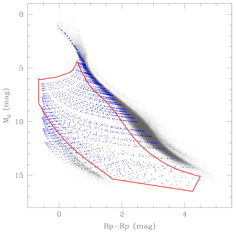
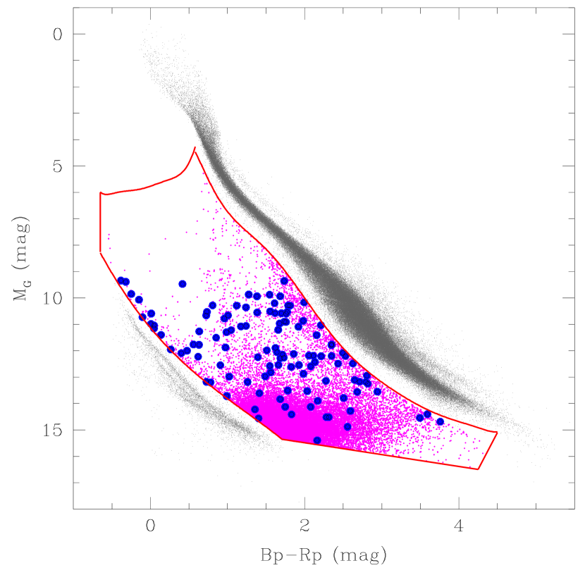
Figure 1: Left panel: Gaia EDR3 main sequence stars and white dwarfs within 100 pc (gray dots), the synthetic WDMS binaries (blue dots) and the colour-magnitude selection of WDMS binaries (red solid lines). The absolute magnitudes and colours of the synthetic WDMS binaries were obtained combining a grid of white dwarf (with effective temperatures and surface gravities ranging from 3 000 to 100 000 K and from 7 to 9.5 dex) and main sequence star (with effective temperatures ranging from 2 400 to 9 700 K) fluxes. See text for details. Right panel: The same as the left panel but showing the WDMS binary candidates (magenta) that result from applying the cuts to the Gaia EDR3 data base. The final sample after excluding contaminants is shown as blue solid dots.

Conversely, for smaller initial main sequence binary separations, mass transfer interactions ensue, which generally lead to a common envelope phase and to a dramatic shrinkage of the orbit (Willems & Kolb, 2004). These close binaries are commonly referred to as post-common envelope binaries or PCEBs. Once they are formed, these objects are subject to substantial angular momentum loss due to gravitational radiation and/or magnetic braking, which make their orbital periods shorter. Hence, they are the progenitors of a wide range of important outcomes, e.g. type Ia supernovae, double degenerate binaries, white dwarf pulsars (Toloza et al., 2019) or highly-field magnetic white dwarfs (García-Berro et al., 2012). PCEBs have played a very important role in studying a wide variety of open problems in modern astronomy. These include constraining the efficiency of common envelope evolution and its energy budget (Zorotovic et al., 2010; Rebassa-Mansergas et al., 2012b; Camacho et al., 2014; Zorotovic et al., 2014), confirming the inefficiency of magnetic braking for fully convective stars (Schreiber et al., 2010; Zorotovic et al., 2016), proving that the origin of low-mass ($\la 0.45\,$M_⊙) white dwarfs is mainly a consequence of binary evolution (Rebassa-Mansergas et al., 2011), constraining the secondary star mass function (Ferrario, 2012; Cojocaru et al., 2017), as well as testing the mass-radius relation of white dwarfs (Parsons et al., 2017), main sequence stars (Parsons et al., 2018) and metal-poor sub-dwarf stars (Rebassa-Mansergas et al., 2019a) via the analysis of eclipsing binaries.

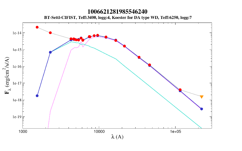
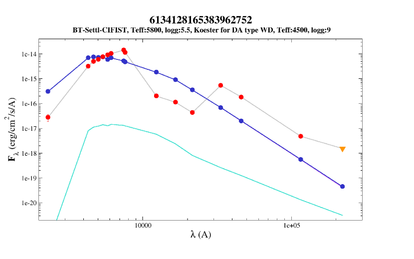
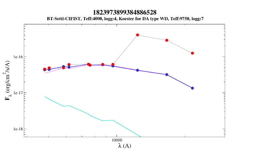
Figure 2: Different examples of bad two-body SED fittings with VOSA. From left to right and from top to bottom: Bad UV fit, bad photometry, and contamination from a nearby star at WISE wavelengths. The cyan and magenta lines represent the hydrogen-rich white dwarf (Koester, 2010) and CIFIST main sequence star (Baraffe et al., 2015) models, respectively. Red dots are the observed photometric points while the blue line and dots indicate the composite model that best fits the data. The yellow inverted triangles indicate that the photometric values correspond to upper limits and, thus, are not taken into account in the fitting process.

Behind all the important results derived analysing both wide WDMS binaries and PCEBs relies a tremendous observational effort dedicated to identifying large and homogeneous (i.e. selected under the same criteria) samples of such systems. So far, the largest and most homogeneous catalogues of spectroscopic WDMS binaries have been obtained from the Sloan Digital Sky Survey (SDSS; York et al. 2000; Eisenstein et al. 2011) (Rebassa-Mansergas et al., 2010; Rebassa-Mansergas et al., 2012a; Rebassa-Mansergas et al., 2013b; Rebassa-Mansergas et al., 2016a) and the Large Sky Area Multi-Object Fiber Spectroscopic Telescope (LAMOST; Cui et al. 2012; Chen et al. 2012) Survey (Ren et al., 2014, 2018). Counting the SDSS sample with $\simeq$3 200 systems and the LAMOST sample with $\simeq$900 objects, both catalogues have been prolific at revealing a large number of radial velocity variable, i.e. PCEBs, and non-variable systems (Rebassa-Mansergas et al., 2007; Rebassa-Mansergas et al., 2011; Schreiber et al., 2008; Schreiber et al., 2010) –and the corresponding orbital period distributions (Rebassa-Mansergas et al., 2008; Nebot Gómez-Morán et al., 2011) – as well as of eclipsing binaries (Parsons et al., 2012, 2013, 2015; Pyrzas et al., 2009, 2012; Rebassa-Mansergas et al., 2016a; Rebassa-Mansergas et al., 2019a).

However, it is important to emphasise that both the SDSS and LAMOST WDMS binary catalogues are heavily affected by selection effects (Rebassa-Mansergas et al., 2010; Ren et al., 2018). For instance, being the SDSS a dedicated survey to spectroscopically follow-up quasars and galaxies, the resulting WDMS binary catalogue is biased against the identification of cool white dwarfs (the dominant underlying population) and is dominated by systems containing hot white dwarfs ($\ga$10 000 K), which overlap with quasars in colour space. Cooler white dwarfs are also under-represented in the LAMOST WDMS binary catalogue (Ren et al., 2018) because of their intrinsic faintness. Moreover, the identification of both components relies on the visual inspection of the spectra, which makes it virtually impossible to identify WDMS binaries when one of the stars dominates the spectral energy distribution (SED) at optical wavelengths. As a consequence, the WDMS binary sample mainly consists of secondary stars of spectral type M. Fortunately, a step forward in this line has been possible thanks to the combination of optical spectroscopy (from LAMOST or RAVE, the Radial Velocity Experiment; Kordopatis et al. 2013; Kunder et al. 2017) and/or astrometry (from TGAS, the Tycho-Gaia astrometric solution; Michalik et al. 2015 and Gaia DR2; Evans et al. 2018) with ultraviolet photometry (from GALEX, Galaxy Evolution Explorer; Martin et al. 2005), which has allowed identifying large samples of WDMS binary candidates containing earlier type A, F, G and K companions (Parsons et al., 2016; Rebassa-Mansergas et al., 2017; Ren et al., 2020; Anguiano et al., 2020). Finally, the SDSS and LAMOST catalogues are magnitude-limited samples and, as a consequence, it is difficult to derive space densities of both wide WDMS binaries and PCEBs.

Thanks to the parallaxes provided by the Gaia mission (Gaia Collaboration et al., 2016a; Gaia Collaboration et al., 2020) the prospects of obtaining statistically large and homogeneous volume-limited samples have dramatically increased. For example, the 100 pc volume-limited, nearly-complete ($\simeq$95 per cent) Gaia white dwarf sample consist of $\simeq$13 000 objects (Jiménez-Esteban et al., 2018; Gentile Fusillo et al., 2019; Kilic et al., 2020), which is two orders of magnitudes larger than previous catalogues (e.g. Giammichele et al., 2012; Holberg et al., 2016). Comprehensive samples of accreting white dwarfs in cataclysmic variables (Abril et al., 2020; Pala et al., 2020; Abrahams et al., 2020), extremely low-mass white dwarfs (Pelisoli & Vos, 2019), hot subdwarfs (Geier et al., 2019), white dwarfs with infrared excess typical of circumstellar debris disks (Rebassa-Mansergas et al., 2019b; Xu et al., 2020), and white dwarfs that are members of common proper motion pairs (El-Badry & Rix, 2018; El-Badry et al., 2021), have also been obtained from analysing the Gaia data. More recently, Inight et al. (2021) have illustrated the importance of defining a volume-limited sample of close white dwarf binaries. Our motivation in this work is to identify a sample of unresolved white dwarf binaries within 100 pc, in particular those having main sequence companions, i.e. WDMS. At this maximum distance we expect the selected targets to form a nearly-complete sample (Jiménez-Esteban et al., 2018). Moreover, being these WDMS binaries unresolved in Gaia, it is expected that a relatively large fraction of them should have evolved through a common envelope phase. This is because the majority of wide binaries that evolved avoiding mass transfer episodes are expected to be partially or fully resolved at such short distances. Thus, by analysing this nearly-complete volume-limited sample we are able to derive an upper estimate of the space density of PCEBs. Unlike Belokurov et al. (2020), who made use of the renormalised unit weight error (RUWE) to identify unresolved binaries, we define specific colour-magnitude cuts to select unresolved WDMS binary candidates. By applying the two-body fitting algorithm implemented in VOSA (Virtual Observatory SED Analyser; Bayo et al. 2008) to the selected candidates, we are able to exclude contaminants and to determine the white dwarf and main sequence star stellar parameters, which are compared to those obtained from the SDSS WDMS magnitude-limited catalogue (Rebassa-Mansergas et al., 2010; Rebassa-Mansergas et al., 2016a).

2 The selection of unresolved WDMS binaries

In the Hertzsprung-Russell (HR) diagram, unresolved WDMS binaries are expected to form a bridge between the main sequence star and the white dwarf star loci if there is sufficient flux from both components. Otherwise, the flux of one of the stars dominates the SED and, as we have already mentioned, these binaries are extremely difficult to identify because they have similar magnitudes and colours as single stars. We searched for unresolved WDMS binary candidates in which the two components emit sufficient flux to be individually detected in the SEDs as follows.

First, we derived synthetic WDMS binary $G$ absolute magnitudes and $G_{\mathrm{BP}}-G_{\mathrm{RP}}$ colours. We did this converting the Gaia EDR3 absolute magnitudes that we incorporated in the hydrogen-rich white dwarf cooling sequences of La Plata group (Althaus et al., 2013; Camisassa et al., 2016; Camisassa et al., 2019) to fluxes and combining them with the main sequence star (spectral types A to M) fluxes that we obtained from transforming the absolute magnitudes provided by the updated tables of Pecaut & Mamajek (2013). We then converted the combined fluxes back into absolute magnitudes and thus obtained a grid of synthetic WDMS binary $G$ absolute magnitudes and $G_{\mathrm{BP}}-G_{\mathrm{RP}}$ colours. The grid contained 28 944 points with white dwarf effective temperatures and surface gravities ranging from 3 000 to 100 000 K and from 7 to 9.5 dex, respectively, and main sequence star effective temperatures ranging from 2 400 to 9 700 K. As expected, those synthetic WDMS binaries with a white dwarf (main sequence star) dominant component had associated magnitudes nearly identical to those of single white dwarfs (main sequence stars).

Second, we implement a set of cuts for selecting WDMS binaries based on the position of the synthetic $G$ absolute magnitudes and $G_{\mathrm{BP}}-G_{\mathrm{RP}}$ colours in the HR diagram (see Fig. 1, left panel). These cuts were developed to exclude single white dwarfs and main sequence stars (unfortunately, these also excluded WDMS binaries in which one of the stars dominates the SED), thus selecting WDMS binary candidates in which the two components are expected to contribute to the SEDs. We note that the synthetic main sequence absolute magnitudes are provided for the Gaia DR2 filters by Pecaut & Mamajek (2013). However, as can be seen in the left panel of Figure 1, the position of synthetic WDMS binaries with negligible white dwarf fluxes perfectly coincides with the main loci of observed EDR3 single main sequence stars. Since the main purpose here is to apply cuts for excluding single stars, we consider that using synthetic Gaia DR2 magnitudes for main sequence stars has no major impact in our analysis.

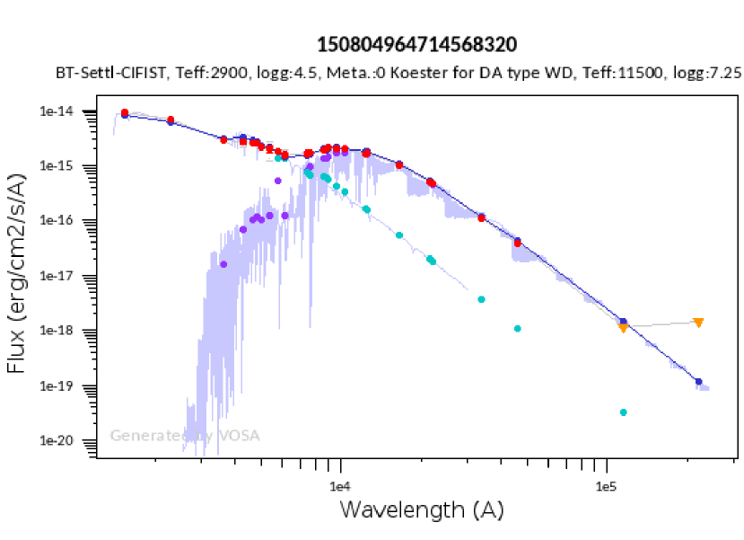
Figure 3: Composite SED of the source Gaia_EDR3_ID: 150804964714568320. The cyan dots and the corresponding purple line represent the hydrogen-rich white dwarf Koester model while the purple dots and the corresponding purple line indicate the CIFIST model. The rest of symbols and colours as in Fig. 2.

The cuts for selecting WDMS binary candidates are illustrated in Figure 1 as red solid lines and follow these equations:

$$[(M_{\mathrm{G}}>5.76332-1.00990(G_{\mathrm{BP}}-G_{\mathrm{RP}})$$

$$-0.78017(G_{\mathrm{BP}}-G_{\mathrm{RP}})^{2}+4.21489(G_{\mathrm{BP}}-G_{\mathrm{RP}})^{3}$$

$$+1.71673(G_{\mathrm{BP}}-G_{\mathrm{RP}})^{4}-25.49710(G_{\mathrm{BP}}-G_{\mathrm{RP}})^{5}$$

$$-13.68387(G_{\mathrm{BP}}-G_{\mathrm{RP}})^{6}+24.16992(G_{\mathrm{BP}}-G_{\mathrm{RP}})^{7}$$

$$\hskip 5.69046pt\mathrm{AND}\hskip 5.69046pt-0.65<(G_{\mathrm{BP}}-G_{\mathrm{RP}})<0.58)$$

$$\mathrm{OR}$$

$$(M_{\mathrm{G}}>21.22759-118.35415(G_{\mathrm{BP}}-G_{\mathrm{RP}})$$

$$+305.43033(G_{\mathrm{BP}}-G_{\mathrm{RP}})^{2}-393.13909(G_{\mathrm{BP}}-G_{\mathrm{RP}})^{3}$$

$$+294.22156(G_{\mathrm{BP}}-G_{\mathrm{RP}})^{4}-135.40159(G_{\mathrm{BP}}-G_{\mathrm{RP}})^{5}$$

$$+38.90143(G_{\mathrm{BP}}-G_{\mathrm{RP}})^{6}-6.80771(G_{\mathrm{BP}}-G_{\mathrm{RP}})^{7}$$

$$+0.66434(G_{\mathrm{BP}}-G_{\mathrm{RP}})^{8}-0.02773(G_{\mathrm{BP}}-G_{\mathrm{RP}})^{9}$$

$$\hskip 5.69046pt\mathrm{AND}\hskip 5.69046pt0.58\leq(G_{\mathrm{BP}}-G_{\mathrm{RP}})<4.5)]$$ (1)

AND

$$[(M_{\mathrm{G}}<11.13367+3.51045(G_{\mathrm{BP}}-G_{\mathrm{RP}})$$

$$-1.13132(G_{\mathrm{BP}}-G_{\mathrm{RP}})^{2}+0.30628(G_{\mathrm{BP}}-G_{\mathrm{RP}})^{3}$$

$$\hskip 5.69046pt\mathrm{AND}\hskip 5.69046pt-0.65<(G_{\mathrm{BP}}-G_{\mathrm{RP}})<1.7)$$

$$\hskip 5.69046pt\mathrm{OR}\hskip 5.69046pt$$

$$(M_{\mathrm{G}}<14.587+0.45098(G_{\mathrm{BP}}-G_{\mathrm{RP}})$$

$$\hskip 5.69046pt\mathrm{AND}\hskip 5.69046pt1.7\leq(G_{\mathrm{BP}}-G_{\mathrm{RP}})<4.25)$$

$$\hskip 5.69046pt\mathrm{OR}\hskip 5.69046pt$$

$$(M_{\mathrm{G}}<40.3-5.6(G_{\mathrm{BP}}-G_{\mathrm{RP}})$$

$$\hskip 5.69046pt\mathrm{AND}\hskip 5.69046pt4.25\leq(G_{\mathrm{BP}}-G_{\mathrm{RP}})<4.5))]$$ (2)

We used the above cuts to select WDMS binary candidates within Gaia EDR3, together with the following conditions that we applied in order to ensure good quality in the photometric and astrometric values:

• 1/$\varpi\leq$ 100

• $\varpi/\sigma_{\varpi}\geq$ 10

• $I_{\rm BP}/\sigma_{I_{\rm BP}}\geq$ 10

• $I_{\rm RP}/\sigma_{I_{\rm RP}}\geq$ 10

• $I_{\rm G}/\sigma_{I_{\rm G}}\geq$ 10

where $\varpi$ is the parallax in arcseconds, $I_{\rm G}$, $I_{\rm BP}$ and $I_{\rm RP}$ are the fluxes in the bandpass filters $G$, $G_{\mathrm{BP}}$ and $G_{\mathrm{RP}}$ respectively and the $\sigma$ values are the standard errors of the corresponding parameters. This resulted in 20 719 WDMS binary candidates, which are illustrated in the right panel of Figure 1. As it can be seen from inspection of this Figure, there seems to be a large number of false positive candidates, mainly due to the fact that we did not apply any condition on the excess flux factor. While the flux in the $G$ band is determined from a profile-fitting, the $BP$ and $RP$ fluxes are computed by summing the flux in a field of 3.5 $\times$ 2.1 arcsec² (Evans et al., 2018). Given the $G_{\mathrm{BP}},G_{\mathrm{RP}}$ and $G$ passbands, the sum of $G_{\mathrm{BP}}$ and $G_{\mathrm{RP}}$ fluxes should exceed the $G$ flux by only a small factor. Larger deviations should be caused by contamination from nearby sources or bright background in the $G_{\mathrm{BP}}$ and $G_{\mathrm{RP}}$ bands.

In order to quantify this effect, Evans et al. (2018) defined the excess factor as the flux ratio  C = ($I_{\mathrm{BP}}$ +$I_{\mathrm{RP}}$) / $I_{\mathrm{G}}$ . However, as Riello et al. (2020) pointed out, there is a clear colour dependence of the excess factor that is not taken into account in the previous expression. To overcome this situation, they introduced a corrected excess factor defined as C^∗ = C - f($G_{\mathrm{BP}},G_{\mathrm{RP}}$) where f($G_{\mathrm{BP}},G_{\mathrm{RP}}$) is a function providing the expected excess at a given colour. According to this, a C^∗ value close to zero would indicate that the source is not affected by excess flux in the $G_{\mathrm{BP}}$ or $G_{\mathrm{RP}}$ band.

Using C^∗ and adequate values of sigma – the scatter of C^∗ as a function of the $G$ magnitude, see Eq. 18 in Riello et al. (2020) – we ended up with 2 001 sources with consistent photometric values in the $G_{\mathrm{BP}},G_{\mathrm{RP}}$ and $G$ filters. It is possible that a fraction of the objects we have excluded because of the excess factor criteria are real but partially resolved WDMS binaries. However, we emphasise that the goal of this work is to identify unresolved WDMS binaries.

3 Stellar parameters of the final unresolved WDMS binary sample

We executed VOSA to estimate the stellar parameters of the 2 001 candidates selected in the previous Section. Firstly, we built the SED of the objects from the UV to the mid-IR using the public catalogues accessible within VOSA. In particular we used GALEX GR6+7 (Bianchi et al., 2017), APASS DR9 (Henden et al., 2015), SDSS DR12 (Alam et al., 2015), Pan-Starrs PS1 DR2 (Magnier et al., 2020), Gaia EDR3 (Gaia Collaboration et al., 2021, 2016b), 2MASS PSC (Skrutskie et al., 2006), and AllWISE (Wright et al., 2010). VOSA gathers not only the photometric information (magnitudes and errors) but also the associated quality flags. This way, photometric points with poor quality were removed before the SED fitting. Also, upper limits were not considered either.

Given that our targets are close objects ($\leq 100$ pc), proper motions are expected to be high. We took them into account by computing the coordinates of the targets in the epoch 2000 using the astrometric information provided by Gaia, and then applied a 5 arcsec search radius around the epoch 2000 coordinates.

For 70 sources, the number of collected photometric measurements was too small to carry out the SED fitting. After visual inspection we discarded another 302 sources having wrong photometric values. The rest (1 629) were fitted using either the main sequence star BT-Settl CIFIST (Baraffe et al., 2015) or the hydrogen-rich white dwarf (Koester, 2010) collections of theoretical models. In total, 1 349 objects had a good SED fitting (vgfb$<$15), indicating that their SEDs resemble those of single stars. vgfb is a modified $\chi^{2}$, internally used by VOSA, that is calculated by forcing $\Delta F_{\mathrm{i}}$ to be larger than 0.1 $\times F_{\mathrm{i}}$, where $\Delta F_{\mathrm{i}}$ is the error in the observed $F_{\mathrm{i}}$ for the $i$-th flux in the SED. This parameter is particularly useful when the photometric errors of any of the catalogues used to build the SED are underestimated. vgfb$<$ 15 is a reliable indicator of good fit. The remaining 280 (1 629-1 349) are candidates to WDMS binary systems. For these objects we took advantage of the two-body fitting capabilities implemented in VOSA. 129 objects could not be fitted due to, at least, one of the following three reasons: UV excess likely due to stellar activity of the main sequence companion, bad SED fitting or contamination from a nearby star, in particular at WISE wavelengths. In Figure 2 we show an example for each of the previous cases. In order to ensure that our sample is actually within 100 pc from the Sun, we removed from the remaining 151 (280-129) objects those having bad astrometry (RUWE>2 or astrometric_-excess_-noise>2 and astrometric_-excess_-noise_-sig>2). After this, we ended up with a final list of 117 good candidates to WDMS binaries within 100 pc. An example of the SED fitting of one of these sources is shown in Figure 3.

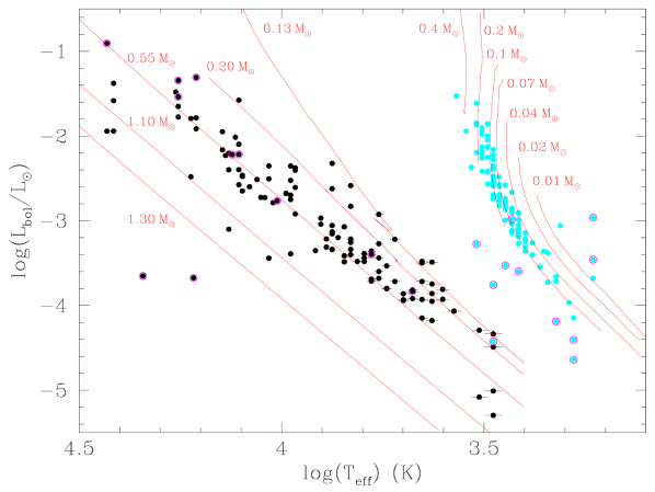
Figure 4: Luminosities as a function of effective temperatures for the 117 white dwarfs (black solid dots) and their companions (cyan solid dots) that are part of unresolved WDMS binary candidates and with good two-body VOSA fits. The solid red lines show the hydrogen-rich white dwarf theoretical relations for fixed masses of 0.13 M_⊙ and 0.20 M_⊙ (Calcaferro et al., 2018), 0.55 M_⊙ (Camisassa et al., 2016) and 1.1 M_⊙ and 1.3 M_⊙(Camisassa et al., 2019), the main sequence theoretical relations for a fixed mass of 0.40 M_⊙, 0.20 M_⊙, 0.10 M_⊙ and 0.07 M_⊙ (Baraffe et al., 2015) and the brown dwarf theoretical relations for 0.04 M_⊙, 0.02 M_⊙ and 0.01 M_⊙ (CIFIST models). The pairs for which at least one of the components has a temperature-luminosity observed relation which is far away from the theoretical expected values are surrounded by magenta open circles.

For the 117 unresolved WDMS binary candidates with good two-body fits VOSA provides information, for each component, on effective temperatures ($T_{\rm eff}$) and total bolometric fluxes ($F_{\mathrm{bol}}$). The temperatures are estimated from the model that best fits the data after the appropriate re-scaling in flux. For a detailed description on how the total bolometric flux is computed see the VOSA documentation. Luminosities are then obtained from the equation

$$L_{\mathrm{bol}}(L_{\odot})=4\pi D^{2}F_{\mathrm{bol}}$$ (3)

where $L_{\mathrm{bol}}$ is the bolometric luminosity (luminosity, hereafter), that is, the total amount of electromagnetic energy emitted per unit of time and $D$ represents the distance in parsecs obtained from the inverse of the Gaia parallax. In Figure 4 we show these luminosities as a function of the effective temperatures derived from the best-model fits for both the white dwarfs and their companions. For comparison, we also represent the theoretical $L_{\mathrm{bol}}$ versus $T_{\mathrm{eff}}$ relations for different white dwarf and main sequence star and brown dwarf masses. As it can be seen from the figure, the $L_{\mathrm{bol}}$ and $T_{\mathrm{eff}}$ values measured by VOSA fall in the expected region for the white dwarfs, except in two cases in which the luminosities are too low for the expected effective temperatures. For a companion to one of these two white dwarfs, as well as in 9 more cases, the observed parameters of the main sequence stars are also clearly away from the expected theoretical values (See Figure 4). One possible explanation for this discrepancy is the existence of another component, for instance an accretion disk as in cataclysmic variables, which has not been taking into account in our analysis. Consequently, given the lack of spectroscopy we cannot confirm or disprove the nature of these 11 objects to be real WDMS binaries and therefore we decided to consider them as candidates with unreliably determined stellar parameters. These objects are represented by open magenta circles in Figure 4.

Radii are estimated by VOSA using the following two independent equations for each component:

$$R_{1}=\sqrt{D^{2}M_{\mathrm{D}}}\\$$ (4)

where M_D is the scaling factor of the model fluxes to fit the observed ones, and

$$R_{2}=\sqrt{L_{\mathrm{bol}}/(4\pi\sigma_{SB}T_{\mathrm{eff}}^{4})}$$ (5)

where $\sigma_{SB}$ is the Stefan-Boltzmann constant, with a value of 5.67 $\times$10^-8 W m^-2 K^-4. Both expressions return almost identical values for the radii and we adopt those resulting from Eq. (5).

Figure 5: Comparison between the white dwarf stellar parameters (mass, effective temperature and surface gravity) and secondary star effective temperatures derived for the WDMS components in the Gaia (black) and SDSS (gray) samples. The left panels show the cumulative distributions; the right panels the normal distributions.

Once the effective temperatures and radii of both stellar components are determined from the VOSA two-body SED fitting, we obtain the surface gravities of the white dwarfs by interpolating the corresponding $T_{\mathrm{eff}}$ and $R$ values in the (hydrogen-rich) cooling sequences of the La Plata group: Althaus et al. (2013) and Calcaferro et al. (2018, we adopted the tracks with a thin hydrogen envelope) for low-mass and extremely low-mass He-core white dwarfs, respectively, Camisassa et al. (2016) for CO-core white dwarfs and Camisassa et al. (2019) for ONe-core white dwarfs. It is worth mentioning that the evolutionary sequences of extremely low-mass white dwarfs are rather complicated, as these objects undergo hydrogen flash phases that move them back and forth and up and down in the $\log(L_{\mathrm{bol}})$-$\log(T_{\mathrm{eff}})$ diagram (see e.g. Figure 1 of Istrate et al., 2016). We assume our extremely low-mass white dwarfs to have already passed these flashes and to be in the final stage of their cooling, which is a good assumption given the low effective temperatures and luminosities measured by the VOSA fitting. The white dwarf masses are then easily derived from the surface gravity and radius determinations. For three WDMS binary candidates (IDs 2630815357409558400, 4550719958390541824 and 2027615341341444608) the white dwarf masses were estimated to be lower than the 0.13$\,M_{\odot}$ lowest limit from our theoretical models.

We cross-matched our 117 Gaia WDMS binary candidates with the SIMBAD database (Wenger et al., 2000) in order to identify the already known sources and collect information about their nature. For this we computed the coordinates of the targets in the epoch J2000 using the astrometric information provided by Gaia, and then applied a 3 arcsec search radius around the epoch J2000 coordinates. Of the 117 WDMS candidates, 20 were already identify as binary systems, five of them as cataclysmic variables (Table 1; note that for these targets the luminosities and effective temperatures derived by VOSA, also included in the table, were in agreement with the expected theoretical values in Figure 4). Two of these cataclysmic variables (Gaia EDR3 6185040879503491584 and 783921244796958208) were also included in Pala et al. (2020). The remaining 97 objects are hence new identifications as WDMS binary candidates.

Table 1: List of cataclysmic variables reported in SIMBAD and included in our list of 117 WDMS binary candidates. The last two columns indicate the luminosities and effective temperatures derived by VOSA for the white dwarf and main sequence star components.

Gaia ID EDR3	RA	DEC	log($L_{\mathrm{bol}}$)WD	log($T_{\mathrm{eff}}$)WD	log($L_{\mathrm{bol}}$)MS	log($T_{\mathrm{eff}}$)MS
	(J2016)	(J2016)	($L_{\odot}$)	(K)	($L_{\odot}$)	(K)
5034416735723964800	14.87104	-26.51935	3.86	-3.20	3.48	-2.693
6185040879503491584	193.10032	-29.24875	4.11	-1.57	3.50	-2.416
674214551557961984	118.77167	22.00122	4.26	-1.48	3.57	-1.527
755705822218381184	156.61466	38.75055	4.13	-3.10	3.50	-2.259
783921244796958208	168.93529	42.97289	4.41	-1.58	3.48	-2.547

For the 15 (20-5) objects reported in SIMBAD as WDMS, the spectral types of the M dwarf companions are provided for three of them. The temperatures obtained by VOSA for these sources were in agreement with the tabulated spectral types by SIMBAD, using the correspondence between spectral type and effective temperature for dwarf stars in Pecaut & Mamajek (2013).

We also cross-matched our Gaia sample of WDMS candidates with the SDSS WDMS binary catalogue within 100 pc. Seven SDSS WDMS binaries fulfilled all the criteria used to select our Gaia sample. All of them were identified by our methodology. In the same way, we checked if the 13 PCEBs from Schreiber & Gänsicke (2003) that are presumably located below 100 pc were in our list. Of these, 6 were not included in our original selection of 20 179 objects (Section 2); 4 because the Gaia EDR3 distances are actually larger than 100 pc and the other 2 because they are not within our WDMS region in the HR diagram (they are located on the main sequence). The remaining 7 objects were picked up by our selection, however one of them had bad photometry and three more had bad 2-body VOSA fits and were therefore excluded (see Figure 2).

Finally, we searched for available public spectra of our 117 sources and found 28 matches. The spectra were obtained from the SDSS archive and from the LAMOST and ESO VO services using the SVO Discovery Tool. Inspection of the spectra and their SEDs revealed all our targets to be genuine WDMS binaries except one system which turned out to be one of the known cataclysmic variables included in Table 1 (Gaia EDR3 783921244796958208).

After excluding the identified cataclysmic variables, our final sample of unresolved Gaia WDMS binary candidates is reduced to 112 (117-5) sources and for 98 of them (excluding the 11 magenta open circle pairs in Fig. 4 and the 3 systems with estimated white dwarf masses lower than 0.13 $M_{\odot}$) the stellar parameters are considered to be reliable. The stellar parameters, the SED two-body fits and the information for each of these 112 WDMS binary candidates can be found at the SVO archive of WDs (see Appendix A).

4 Comparison between the SDSS and the Gaia WDMS binary samples

In the previous section we have identified 112 unresolved Gaia WDMS binary candidates within 100 pc and measured their stellar parameters. For 98 of them we found the derived parameters to be consistent with the theoretical expectations. Here we compare the resulting stellar parameter distributions of these 98 objects (namely the white dwarf effective temperatures, surface gravities and masses, and secondary star effective temperatures) to those from the magnitude-limited SDSS sample. We note that in this exercise we considered SDSS WDMS binaries consisting of a hydrogen-rich white dwarf and a M dwarf companion, since these are the only systems for which the full set of stellar parameters is available (Rebassa-Mansergas et al., 2010). Moreover, we excluded SDSS WDMS binaries displaying no significant radial velocity variations, i.e non-PCEBs. This was required since the majority of unresolved Gaia WDMS binaries have evolved through a common envelope phase and are now close compact binaries (see further details in Section 5.1), and the properties of close PCEBs and wide WDMS are statistically different (Rebassa-Mansergas et al., 2011).

The right panels of Figure 5 show the stellar parameter distributions arising from the two samples. It has to be noted that spectral types, and not effective temperatures, are provided for the M dwarf companions of the SDSS sample. For a proper comparison, we converted these into effective temperatures using the updated tables of Pecaut & Mamajek (2013). Inspection of the figure reveals that the properties of Gaia WDMS binaries seem to be rather different than those of the SDSS ones, as expected from a comparison between a volume-limited and a magnitude-limited sample. The cumulative stellar parameter distributions for both samples are illustrated in the left panels of Figure 5. We run Kolmogorov-Smirnov (KS) tests to the white dwarf cumulative parameter distributions to evaluate the probability that the two samples are drawn from the same parent population. Since the secondary star effective temperature values are discrete for both samples, we run a $\chi^{2}$-test in this case. Not surprisingly, the probabilities we obtained were of the order of less than $10^{-4}$ ($>3.5\sigma$ significance) in all cases.

To begin with, the Gaia sample contains a considerably larger fraction of cool ($<10\,000$ K) white dwarfs. Such white dwarfs, being fainter, are intrinsically less numerous in a magnitude-limited sample. Moreover, as we have already mentioned, most of the SDSS WDMS binaries were observed because of their similar colours to quasars, which overlap in colour space especially when the white dwarfs are hotter than 10 000 K. The fact that Gaia WDMS binaries contain systematically cooler white dwarfs was already pointed out by Inight et al. (2021).

Figure 6: Simulated HR diagram displaying single white dwarfs and single main sequence stars (grey solid dots), unresolved WDMS binaries (blue solid dots) and unresolved WDMS binaries passing our selection cuts (solid magenta dots). The selection cuts are illustrated as red solid lines.

The white dwarfs in both samples (volume- and magnitude-limited) are systematically less massive than canonical (0.6 M_⊙ – log g=8 dex) single white dwarfs (Hollands et al., 2018; McCleery et al., 2020). This is not surprising since the evolution of a large fraction of these white dwarfs was likely truncated when their progenitors were ascending the giant branch and the systems entered the CE phase. In particular, we can observe a considerably larger number of extremely low-mass (ELM) white dwarfs (M $<0.3$ M_⊙) in the Gaia sample. It is not clear how ELMs with low-mass main-sequence star companions would form. Current evolutionary models of ELMs in double-degenerate systems predict that the formation of ELMs with masses lower than $\simeq$0.20 $M_{\odot}$ is likely due to non-conservative stable mass transfer via Roche-lobe overflow (Sun & Arras, 2018; Li et al., 2019). This is based on the estimated energy that would be required to expel the envelope in a common-envelope scenario, which would be too large and cause the system to eventually merge. However, in our case, the low mass of the main sequence companion would lead to an unstable mass transfer. In this way, if these systems were formed by common-envelope evolution, somehow the energetics should be able to eject the envelope. Up to our knowledge, this scenario has not been explored so far. ELM objects have been efficiently identified in the SDSS as apparently single white dwarfs (Brown et al., 2010, 2012; Brown et al., 2020). This is because ELM white dwarfs have considerably larger radii which, together with the fact that the SDSS seldom targets cool white dwarfs for spectroscopic follow-up, implies that their companions (being these main sequence stars or other white dwarfs) are generally completely out-shined. In the volume-limited Gaia sample, ELM white dwarfs are detected with main sequence companions only if these white dwarfs are sufficiently cool for not to out-shine them. Indeed, ELM white dwarfs in the Gaia sample have effective temperatures in the range 3 000-9 500 K, with an average of 5 600$\pm$2 100 K.

Finally, the comparison between the secondary star effective temperatures reveals that the Gaia sample contains a considerably larger fraction of cool companions ($\la$2800 K). This is a simple consequence of the fact that Gaia allows detecting a larger number of cool white dwarfs in WDMS systems. These cool white dwarfs can only be observed together with cool M stars if both components contribute similarly to the SEDs, otherwise the M dwarfs would overwhelm the fluxes of the white dwarfs. It is important to also note that 8 of these companions have effective temperatures below 2250 K, the commonly accepted limit which separates main sequence stars from brown dwarfs (Pecaut & Mamajek, 2013; Kirkpatrick et al., 2021). Further spectroscopic observations are required to confirm the brown dwarf nature of these objects.

It has to be emphasized that the stellar parameters of the white dwarfs in Gaia WDMS binaries have been obtained using hydrogen-rich (DA) cooling sequences, an assumption that has not been tested due to the lack of spectroscopy. Then, one may expect a fraction of non-DA white dwarfs in the sample (mainly DBs with helium-rich atmospheres, which are the second most common type of white dwarfs after the DAs, see e.g. Koester & Kepler 2015). However, no single PCEB with a DB white dwarf has been found yet, most likely because the white dwarfs in these systems accrete material from the wind arising from their main-sequence companions (Parsons et al., 2013). This material is expected to form a hydrogen layer on the white dwarf’s atmosphere, thus converting a DB into a DA white dwarf.

5 The completeness and the space density of the Gaia unresolved WDMS binary sample

Despite the fact that our Gaia WDMS binary sample is volume-limited, it is not guaranteed to be complete. First of all, this is because we have focused on identifying systems in which the two stellar components contribute in relatively similar amounts of flux to the SEDs. In second place, as in any other observed sample, selection effects may induce some biases in the final sample.

In order to estimate the completeness of the sample as well as to derive a space density of close WDMS binaries, we use a Monte Carlo population synthesis code specifically designed to simulate the single (García-Berro et al., 1999, 2004; Torres et al., 2005; Jiménez-Esteban et al., 2018; Torres et al., 2021) and binary (Camacho et al., 2014; Cojocaru et al., 2017) white dwarf populations in the Galaxy. It is important to point out here that this analysis shall be understood as a first approximation to the estimation of the completeness of the sample. That is because the space parameter of the white dwarf binary population is not fully determined and several discrepancies arise between the observations and the theoretical models (e.g. Toonen et al. 2017). Consequently, it is beyond the scope of the present work to comprehensively analyze the full set of theoretical models. Instead, we will focus on a reference model that will provide us with a first estimate.

Here we present the main ingredients of our population synthesis model and leave the details and the analysis of other models for a forthcoming paper. The single white dwarf population consist in a three-component Galactic model, i.e., thin and thick disk and halo, as described in Torres et al. (2019). To this population we add a binary population implemented through the BSE (Binary Stellar Evolution) code of Hurley et al. (2002) with some updates introduced in Camacho et al. (2014), Cojocaru et al. (2017) and Canals et al. (2018). The code incorporates an exhaustive list of fundamental binary evolution ingredients, such as mass transfer, wind loss, common-envelope evolution, angular-momentum loss, magnetic braking and gravitational wave radiation emission, among other effects. A binary fraction of 50 per cent is adopted. The primary masses of the binary systems are randomly chosen following the initial mass function of Kroupa (2001) (also adopted for the single star population), while secondary masses follow a flat distribution as in Cojocaru et al. (2017). The orbital separations and the eccentricities follow a logarithmically flat distribution (Davis et al., 2010) and a linear thermal distribution (Heggie, 1975), respectively. For those systems that evolve into a common envelope we use the standard $\alpha_{\mathrm{CE}}$-formalism (Iben & Livio, 1993) following the assumptions detailed in Camacho et al. (2014), where $\alpha_{\mathrm{CE}}$ is the efficiency of the orbital energy in ejecting the envelope (assumed to be 0.3; Zorotovic et al. 2010). Systems are then evolved into present time and their Gaia EDR3 magnitudes are computed according to the La Plata tracks for white dwarfs (Section 3) and the PARSEC tracks for main sequence stars (Bressan et al., 2012; Chen et al., 2014). Photometric and astrometric errors are added to the simulated objects following the Gaia’s performance. The synthetic sample is then normalized to $15\,753$, which is the total number of Gaia EDR3 sources found in the white dwarf loci of the Gaia EDR3 HR diagram (i.e. the area defined by the first condition of Equation 2 but extended up to $G_{\mathrm{BP}}-G_{\mathrm{RP}}\leq 2.0$) after applying the same astrometric and photometric selection criteria as that for the WDMS binary population. Finally, we assume as unresolved systems those for which the angular sky separation is smaller than 2 arcsec. In these cases the final magnitudes are obtained from combining the individual fluxes of the two components.

It is worth mentioning that the claimed angular separation to separate pairs of stars by Gaia EDR3 is $\simeq$1.5 arcsec (Gaia Collaboration et al., 2020). This limit can increase to 2 arcsec for samples selected with good astrometric and photometric parameters, as it is our case (Torres et al., in preparation). Hence the adopted value of 2 arcsec in this work.

Once the simulation is carried out, we have a full modeling of the different sub-populations: resolved and unresolved WDMS binaries, as well as resolved and unresolved double degenerate systems. In Figure 6 we show the HR diagram that results from our simulations within 100 pc for the sub-population of interest in this work, i.e. unresolved WDMS binaries.

5.1 The completeness of the Gaia WDMS binary sample

The simulations presented in the previous section allow us to estimate the completeness of the unresolved Gaia WDMS binary sample studied in this work. Inspection of Figure 6 clearly reveals that the vast majority of WDMS binaries are entirely dominated by the flux of the main sequence companion, since their positions in the HR diagram are very similar to those of single main sequence stars. As a consequence, only $\approx 140\pm 12$ (the error arises after the normalization) of all the synthetic unresolved WDMS binaries fall within our cuts, that is $\simeq$9 per cent of the total sample. These 140 objects represent the WDMS binary population that we should have identified in this work using the methods outlined in Sections 2 and  3. Since our sample consists of 112 WDMS binary good candidates, then the completeness can be initially estimated as $\simeq\,80\pm 9$ per cent.

Based on our simulations we conclude that only $\simeq 9$ per cent of the total unresolved WDMS binary population in the Galaxy can be efficiently identified by our method and that our catalogue (which represents the tip of the iceberg) seems to be highly complete. The remaining $\simeq 91$ per cent represent the underlying population of WDMS binaries that are heavily dominated by the flux of the main sequence companion. Detecting such WDMS binaries is a challenging task that requires UV photometry (Maxted et al., 2009; Parsons et al., 2016; Rebassa-Mansergas et al., 2017; Ren et al., 2020; Hernandez et al., 2021) and/or spectroscopy (Parsons et al., 2016).

We also made use of the population synthesis simulation presented here to estimate the expected fraction of wide WDMS binaries that evolved avoiding mass transfer episodes but have angular separations of 2 arcsec or less, i.e. the limit at which we consider the systems to be spatially unresolved. We found that these systems form $\simeq$28 per cent of the total synthetic WDMS binary population within our WDMS selected region in the HR diagram and with distances up to 100 pc.

5.2 The space density of close WDMS binaries

We have identified 112 unresolved WDMS binary candidates within a volume of 100 pc, which translates into a space density of unresolved (likely PCEBs) binaries consisting of a white dwarf plus a main sequence companion of $\simeq(2.7\pm 1.6)\times 10^{-5}$ pc^-3. Given that we can clearly not rule out the possibility that some of our systems are actually wide but unresolved binaries that did not evolve through CE evolution (see previous Section), this value should be considered as an upper limit. Inight et al. (2021), who analysed the SDSS WDMS binary sample observed by Gaia within 300 pc, derived a space density of 1.2–2.5$\times 10^{-6}$ pc^-3, although they claim this result should be multiplied by 3-4 in order to account for the SDSS selection effects. By doing this, one obtains a value of 0.5–1$\times 10^{-5}$ pc^-3, which is lower but of the same order to our estimated value. Schreiber & Gänsicke (2003) analysed a considerably smaller sample of close WDMS binaries and derived a space density of 0.6–3$\times 10^{-5}$ pc^-3, in agreement with our result. If we correct our space density estimate by the completeness of our sample ($\simeq$80), then this value increases to $\simeq(3.3\pm 1.8)\times 10^{-5}$ pc^-3. If we further consider that, based on our simulations, the sample of WDMS binaries analysed in this work represents only $\simeq$9 per cent of the underlying population, then we estimate an upper limit to the total space density of close WDMS binaries of $\simeq(3.7\pm 1.9)\times 10^{-4}$ pc^-3. This represents $\simeq$7 per cent of the white dwarf space density calculated by Jiménez-Esteban et al. (2018).

6 Conclusions

Close binaries consisting of a white dwarf and a main sequence companion, i.e. WDMS binaries, are important objects to constrain a wide variety of open problems in modern astronomy. However, despite the fact that the SDSS has been very prolific at identifying such systems for follow-up studies in the last years, this sample is heavily affected by selection effects. To overcome this issue, in this work we have used the high astrometric and photometric quality of the recent Gaia Early Data Release 3 to identify a volume-limited sample of 112 unresolved ($\simeq$72 per cent of them expected to be close) WDMS binaries within 100 pc. We have measured their stellar parameters (effective temperatures, luminosities, radii, surface gravities and masses) via fitting their SEDs with a two-body fitting algorithm implemented in VOSA. We find that the Gaia volume-limited sample consists of intrinsically cooler white dwarfs and main sequence companions, some of which are in fact expected to be brown dwarfs. Moreover, the Gaia sample reveals a population of extremely low-mass white dwarfs which is absent in the SDSS magnitude-limited sample. Thus, the sample identified here clearly helps in overcoming the selection effects affecting the SDSS population. It has to be emphasised however that follow-up optical spectroscopy is recommended to confirm the hypothesis stated in this work. Using a Monte Carlo population synthesis code we find that $\simeq$91 per cent of the total unresolved WDMS binary population is expected to be fully dominated by the emission of the main sequence companions. Efficiently identifying these systems requires ultraviolet photometry and/or spectroscopy. We also find strong indications that our catalogue, even though it represents a small fraction of the underlying population, is highly complete ($\simeq 80\pm 9$ per cent) and is not affected by important selection effects. Finally, our population synthesis study allows us to estimate an upper limit to the total space density of close WDMS binaries of $\simeq(3.7\pm 1.9)\times 10^{-4}$ pc^-3.

Appendix A Data availability

In order to facilitate the usage of the information included in this paper, an archive system that can be accessed from a webpage or through a Virtual Observatory ConeSearch has been built.

The archive system implements a very simple search interface that permits queries by coordinates and range of effective temperatures, surface gravities, luminosities, radii and masses. The user can also select the maximum number of sources to return (with values from 10 to unlimited). The result of the query is a HTML table with all the sources found in the archive fulfilling the search criteria. The result can also be downloaded as a VOTable or a CSV file.

Detailed information on the output fields can be obtained placing the mouse over the question mark (“?”) located close to the name of the column. The archive also implements the SAMP (Simple Application Messaging) Virtual Observatory protocol. SAMP allows Virtual Observatory applications to communicate with each other in a seamless and transparent manner for the user. This way, the results of a query can be easily transferred to other VO applications, such as, for instance, Topcat.

References

- Abrahams et al. (2020) Abrahams E. S., Bloom J. S., Mowlavi N., Szkody P., Rix H.-W., Ventura J.-P., Brink T. G., Filippenko A. V., 2020, arXiv e-prints, p. arXiv:2011.12253
- Abril et al. (2020) Abril J., Schmidtobreick L., Ederoclite A., López-Sanjuan C., 2020, MNRAS, 492, L40
- Alam et al. (2015) Alam S., et al., 2015, ApJS, 219, 12
- Althaus et al. (2013) Althaus L. G., Miller Bertolami M. M., Córsico A. H., 2013, A&A, 557, A19
- Anguiano et al. (2020) Anguiano B., et al., 2020, Research Notes of the American Astronomical Society, 4, 127
- Baraffe et al. (2015) Baraffe I., Homeier D., Allard F., Chabrier G., 2015, A&A, 577, A42
- Bayo et al. (2008) Bayo A., Rodrigo C., Barrado y Navascués D., Solano E., Gutiérrez R., Morales-Calderón M., Allard F., 2008, A&A, 492, 277
- Belokurov et al. (2020) Belokurov V., et al., 2020, MNRAS, 496, 1922
- Bianchi et al. (2017) Bianchi L., Shiao B., Thilker D., 2017, ApJS, 230, 24
- Boch & Fernique (2014) Boch T., Fernique P., 2014, in Manset N., Forshay P., eds, Astronomical Society of the Pacific Conference Series Vol. 485, Astronomical Data Analysis Software and Systems XXIII. p. 277
- Bonnarel et al. (2000) Bonnarel F., et al., 2000, A&AS, 143, 33
- Bressan et al. (2012) Bressan A., Marigo P., Girardi L., Salasnich B., Dal Cero C., Rubele S., Nanni A., 2012, MNRAS, 427, 127
- Brown et al. (2010) Brown W. R., Kilic M., Allende Prieto C., Kenyon S. J., 2010, ApJ, 723, 1072
- Brown et al. (2012) Brown W. R., Kilic M., Allende Prieto C., Kenyon S. J., 2012, ApJ, 744, 142
- Brown et al. (2020) Brown W. R., et al., 2020, ApJ, 889, 49
- Calcaferro et al. (2018) Calcaferro L. M., Althaus L. G., Córsico A. H., 2018, A&A, 614, A49
- Camacho et al. (2014) Camacho J., Torres S., García-Berro E., Zorotovic M., Schreiber M. R., Rebassa-Mansergas A., Nebot Gómez-Morán A., Gänsicke B. T., 2014, A&A, 566, A86
- Camisassa et al. (2016) Camisassa M. E., Althaus L. G., Córsico A. H., Vinyoles N., Serenelli A. M., Isern J., Miller Bertolami M. M., García-Berro E., 2016, ApJ, 823, 158
- Camisassa et al. (2019) Camisassa M. E., et al., 2019, A&A, 625, A87
- Canals et al. (2018) Canals P., Torres S., Soker N., 2018, MNRAS, 480, 4519
- Catalán et al. (2008) Catalán S., Isern J., García-Berro E., Ribas I., Allende Prieto C., Bonanos A. Z., 2008, A&A, 477, 213
- Chen et al. (2012) Chen L., et al., 2012, Research in Astronomy and Astrophysics, 12, 805
- Chen et al. (2014) Chen Y., Girardi L., Bressan A., Marigo P., Barbieri M., Kong X., 2014, MNRAS, 444, 2525
- Cojocaru et al. (2017) Cojocaru R., Rebassa-Mansergas A., Torres S., García-Berro E., 2017, MNRAS, 470, 1442
- Cui et al. (2012) Cui X.-Q., et al., 2012, Research in Astronomy and Astrophysics, 12, 1197
- Davis et al. (2010) Davis P. J., Kolb U., Willems B., 2010, MNRAS, 403, 179
- Duquennoy & Mayor (1991) Duquennoy A., Mayor M., 1991, A&A, 500, 337
- Eisenstein et al. (2011) Eisenstein D. J., et al., 2011, AJ, 142, 72
- El-Badry & Rix (2018) El-Badry K., Rix H.-W., 2018, MNRAS, 480, 4884
- El-Badry et al. (2021) El-Badry K., Rix H.-W., Heintz T. M., 2021, MNRAS,
- Evans et al. (2018) Evans D. W., et al., 2018, A&A, 616, A4
- Farihi et al. (2010) Farihi J., Hoard D. W., Wachter S., 2010, ApJS, 190, 275
- Ferrario (2012) Ferrario L., 2012, MNRAS, 426, 2500
- Gaia Collaboration et al. (2016a) Gaia Collaboration et al., 2016a, A&A, 595, A1
- Gaia Collaboration et al. (2016b) Gaia Collaboration et al., 2016b, A&A, 595, A1
- Gaia Collaboration et al. (2020) Gaia Collaboration Brown A. G. A., Vallenari A., Prusti T., de Bruijne J. H. J., Babusiaux C., Biermann M., 2020, arXiv e-prints, p. arXiv:2012.01533
- Gaia Collaboration et al. (2021) Gaia Collaboration et al., 2021, A&A, 649, A1
- García-Berro et al. (1997) García-Berro E., Ritossa C., Iben Icko J., 1997, ApJ, 485, 765
- García-Berro et al. (1999) García-Berro E. Torres S., Isern J., Burkert A., 1999, MNRAS, 302, 173
- García-Berro et al. (2004) García-Berro E., Torres S., Isern J., Burkert A., 2004, A&A, 418, 53
- García-Berro et al. (2012) García-Berro E., et al., 2012, ApJ, 749, 25
- Geier et al. (2019) Geier S., Raddi R., Gentile Fusillo N. P., Marsh T. R., 2019, A&A, 621, A38
- Gentile Fusillo et al. (2019) Gentile Fusillo N. P., et al., 2019, MNRAS, 482, 4570
- Giammichele et al. (2012) Giammichele N., Bergeron P., Dufour P., 2012, ApJS, 199, 29
- Heggie (1975) Heggie D. C., 1975, MNRAS, 173, 729
- Henden et al. (2015) Henden A. A., Levine S., Terrell D., Welch D. L., 2015, in American Astronomical Society Meeting Abstracts #225. p. 336.16
- Hernandez et al. (2021) Hernandez M. S., et al., 2021, MNRAS, 501, 1677
- Holberg et al. (2016) Holberg J. B., Oswalt T. D., Sion E. M., McCook G. P., 2016, MNRAS, 462, 2295
- Hollands et al. (2018) Hollands M. A., Tremblay P. E., Gänsicke B. T., Gentile-Fusillo N. P., Toonen S., 2018, MNRAS, 480, 3942
- Hurley et al. (2002) Hurley J. R., Tout C. A., Pols O. R., 2002, MNRAS, 329, 897
- Iben & Livio (1993) Iben Icko J., Livio M., 1993, PASP, 105, 1373
- Inight et al. (2021) Inight K., Gänsicke B. T., Breedt E., Marsh T. R., Pala A. F., Raddi R., 2021, MNRAS,
- Istrate et al. (2016) Istrate A. G., Marchant P., Tauris T. M., Langer N., Stancliffe R. J., Grassitelli L., 2016, A&A, 595, A35
- Jiménez-Esteban et al. (2018) Jiménez-Esteban F. M., Torres S., Rebassa-Mansergas A., Skorobogatov G., Solano E., Cantero C., Rodrigo C., 2018, MNRAS, 480, 4505
- Kilic et al. (2020) Kilic M., Bergeron P., Kosakowski A., Brown W. R., Agüeros M. A., Blouin S., 2020, ApJ, 898, 84
- Kirkpatrick et al. (2021) Kirkpatrick J. D., et al., 2021, ApJS, 253, 7
- Koester (2010) Koester D., 2010, Mem. Soc. Astron. Italiana, 81, 921
- Koester & Kepler (2015) Koester D., Kepler S. O., 2015, A&A, 583, A86
- Kordopatis et al. (2013) Kordopatis G., et al., 2013, AJ, 146, 134
- Kroupa (2001) Kroupa P., 2001, MNRAS, 322, 231
- Kunder et al. (2017) Kunder A., et al., 2017, AJ, 153, 75
- Li et al. (2019) Li Z., Chen X., Chen H.-L., Han Z., 2019, ApJ, 871, 148
- Magnier et al. (2020) Magnier E. A., et al., 2020, ApJS, 251, 6
- Martin et al. (2005) Martin D. C., et al., 2005, ApJ, 619, L1
- Maxted et al. (2009) Maxted P. F. L., Gänsicke B. T., Burleigh M. R., Southworth J., Marsh T. R., Napiwotzki R., Nelemans G., Wood P. L., 2009, MNRAS, 400, 2012
- McCleery et al. (2020) McCleery J., et al., 2020, MNRAS, 499, 1890
- Michalik et al. (2015) Michalik D., Lindegren L., Hobbs D., 2015, A&A, 574, A115
- Moe & Di Stefano (2017) Moe M., Di Stefano R., 2017, ApJS, 230, 15
- Nebot Gómez-Morán et al. (2011) Nebot Gómez-Morán A., et al., 2011, A&A, 536, A43
- Pala et al. (2020) Pala A. F., et al., 2020, MNRAS, 494, 3799
- Parsons et al. (2012) Parsons S. G., et al., 2012, MNRAS, 420, 3281
- Parsons et al. (2013) Parsons S. G., et al., 2013, MNRAS, 429, 256
- Parsons et al. (2015) Parsons S. G., et al., 2015, MNRAS, 449, 2194
- Parsons et al. (2016) Parsons S. G., Rebassa-Mansergas A., Schreiber M. R., Gänsicke B. T., Zorotovic M., Ren J. J., 2016, MNRAS, 463, 2125
- Parsons et al. (2017) Parsons S. G., et al., 2017, MNRAS, 470, 4473
- Parsons et al. (2018) Parsons S. G., et al., 2018, MNRAS, 481, 1083
- Pecaut & Mamajek (2013) Pecaut M. J., Mamajek E. E., 2013, ApJS, 208, 9
- Pelisoli & Vos (2019) Pelisoli I., Vos J., 2019, MNRAS, 488, 2892
- Pyrzas et al. (2009) Pyrzas S., et al., 2009, MNRAS, 394, 978
- Pyrzas et al. (2012) Pyrzas S., et al., 2012, MNRAS, 419, 817
- Raghavan et al. (2010) Raghavan D., et al., 2010, ApJS, 190, 1
- Rebassa-Mansergas et al. (2007) Rebassa-Mansergas A., Gänsicke B. T., Rodríguez-Gil P., Schreiber M. R., Koester D., 2007, MNRAS, 382, 1377
- Rebassa-Mansergas et al. (2008) Rebassa-Mansergas A., et al., 2008, MNRAS, 390, 1635
- Rebassa-Mansergas et al. (2010) Rebassa-Mansergas A., Gänsicke B. T., Schreiber M. R., Koester D., Rodríguez-Gil P., 2010, MNRAS, 402, 620
- Rebassa-Mansergas et al. (2011) Rebassa-Mansergas A., Nebot Gómez-Morán A., Schreiber M. R., Girven J., Gänsicke B. T., 2011, MNRAS, 413, 1121
- Rebassa-Mansergas et al. (2012a) Rebassa-Mansergas A., Nebot Gómez-Morán A., Schreiber M. R., Gänsicke B. T., Schwope A., Gallardo J., Koester D., 2012a, MNRAS, 419, 806
- Rebassa-Mansergas et al. (2012b) Rebassa-Mansergas A., et al., 2012b, MNRAS, 423, 320
- Rebassa-Mansergas et al. (2013a) Rebassa-Mansergas A., Schreiber M. R., Gänsicke B. T., 2013a, MNRAS, 429, 3570
- Rebassa-Mansergas et al. (2013b) Rebassa-Mansergas A., Agurto-Gangas C., Schreiber M. R., Gänsicke B. T., Koester D., 2013b, MNRAS, 433, 3398
- Rebassa-Mansergas et al. (2016a) Rebassa-Mansergas A., Ren J. J., Parsons S. G., Gänsicke B. T., Schreiber M. R., García-Berro E., Liu X. W., Koester D., 2016a, MNRAS, 458, 3808
- Rebassa-Mansergas et al. (2016b) Rebassa-Mansergas A., et al., 2016b, MNRAS, 463, 1137
- Rebassa-Mansergas et al. (2017) Rebassa-Mansergas A., et al., 2017, MNRAS, 472, 4193
- Rebassa-Mansergas et al. (2019a) Rebassa-Mansergas A., Parsons S. G., Dhillon V. S., Ren J., Littlefair S. P., Marsh T. R., Torres S., 2019a, Nature Astronomy, 3, 553
- Rebassa-Mansergas et al. (2019b) Rebassa-Mansergas A., Solano E., Xu S., Rodrigo C., Jiménez-Esteban F. M., Torres S., 2019b, MNRAS, 489, 3990
- Rebassa-Mansergas et al. (2021) Rebassa-Mansergas A., et al., 2021, arXiv e-prints, p. arXiv:2105.13379
- Ren et al. (2014) Ren J. J., et al., 2014, A&A, 570, A107
- Ren et al. (2018) Ren J. J., Rebassa-Mansergas A., Parsons S. G., Liu X. W., Luo A. L., Kong X., Zhang H. T., 2018, MNRAS, 477, 4641
- Ren et al. (2020) Ren J. J., et al., 2020, ApJ, 905, 38
- Riello et al. (2020) Riello M., et al., 2020, arXiv e-prints, p. arXiv:2012.01916
- Sana et al. (2014) Sana H., et al., 2014, ApJS, 215, 15
- Schreiber & Gänsicke (2003) Schreiber M. R., Gänsicke B. T., 2003, A&A, 406, 305
- Schreiber et al. (2008) Schreiber M. R., Gänsicke B. T., Southworth J., Schwope A. D., Koester D., 2008, A&A, 484, 441
- Schreiber et al. (2010) Schreiber M. R., et al., 2010, A&A, 513, L7
- Siegler et al. (2005) Siegler N., Close L. M., Cruz K. L., Martín E. L., Reid I. N., 2005, ApJ, 621, 1023
- Skinner et al. (2017) Skinner J. N., Morgan D. P., West A. A., Lépine S., Thorstensen J. R., 2017, AJ, 154, 118
- Skrutskie et al. (2006) Skrutskie M. F., et al., 2006, AJ, 131, 1163
- Sun & Arras (2018) Sun M., Arras P., 2018, ApJ, 858, 14
- Taylor (2005) Taylor M. B., 2005, in Shopbell P., Britton M., Ebert R., eds, Astronomical Society of the Pacific Conference Series Vol. 347, Astronomical Data Analysis Software and Systems XIV. p. 29
- Taylor (2006) Taylor M. B., 2006, in Gabriel C., Arviset C., Ponz D., Enrique S., eds, Astronomical Society of the Pacific Conference Series Vol. 351, Astronomical Data Analysis Software and Systems XV. p. 666
- Toloza et al. (2019) Toloza O., et al., 2019, BAAS, 51, 168
- Toonen et al. (2017) Toonen S., Hollands M., Gänsicke B. T., Boekholt T., 2017, A&A, 602, A16
- Torres et al. (2005) Torres S., García-Berro E., Isern J., Figueras F., 2005, MNRAS, 360, 1381
- Torres et al. (2019) Torres S., Cantero C., Rebassa-Mansergas A., Skorobogatov G., Jiménez-Esteban F. M., Solano E., 2019, MNRAS, 485, 5573
- Torres et al. (2021) Torres S., Rebassa-Mansergas A., Camisassa M. E., Raddi R., 2021, MNRAS, 502, 1753
- Veras et al. (2018) Veras D., Xu S., Rebassa-Mansergas A., 2018, MNRAS, 473, 2871
- Wenger et al. (2000) Wenger M., et al., 2000, A&AS, 143, 9
- Willems & Kolb (2004) Willems B., Kolb U., 2004, A&A, 419, 1057
- Winters et al. (2019) Winters J. G., et al., 2019, AJ, 157, 216
- Wright et al. (2010) Wright E. L., et al., 2010, AJ, 140, 1868
- Xu et al. (2020) Xu S., Lai S., Dennihy E., 2020, ApJ, 902, 127
- York et al. (2000) York D. G., et al., 2000, AJ, 120, 1579
- Zhao et al. (2012) Zhao J. K., Oswalt T. D., Willson L. A., Wang Q., Zhao G., 2012, ApJ, 746, 144
- Zorotovic et al. (2010) Zorotovic M., Schreiber M. R., Gänsicke B. T., Nebot Gómez-Morán A., 2010, A&A, 520, A86
- Zorotovic et al. (2014) Zorotovic M., Schreiber M. R., García-Berro E., Camacho J., Torres S., Rebassa-Mansergas A., Gänsicke B. T., 2014, A&A, 568, A68
- Zorotovic et al. (2016) Zorotovic M., et al., 2016, MNRAS, 457, 3867