Large-eddy simulations of marine boundary-layer clouds associated with cold air outbreaks during the ACTIVATE campaign– part 1: Case setup and sensitivities to large-scale forcings

Abstract

Large-eddy simulation (LES) is able to capture key boundary-layer (BL) turbulence and cloud processes. Yet, large-scale forcing and surface turbulent fluxes of sensible and latent heat are often poorly prescribed for LES simulations. We derive these quantities from measurements and reanalysis obtained for two cold air outbreak (CAO) events during Phase I of the Aerosol Cloud meTeorology Interactions oVer the western ATlantic Experiment (ACTIVATE) in February-March 2020. We study the two contrasting CAO cases by performing LES and test the sensitivity of BL structure and clouds to large-scale forcings and turbulent heat fluxes. Profiles of atmospheric state and large-scale divergence and surface turbulent heat fluxes obtained from the reanalysis data ERA5 agree reasonably well with those derived from ACTIVATE field measurements for both cases at the sampling time and location. Therefore, we adopt the time evolving heat fluxes, wind and advective tendencies profiles from ERA5 reanalysis data to drive the LES. We find that large-scale thermodynamic advective tendencies and wind relaxations are important for the LES to capture the evolving observed BL meteorological states characterized by the hourly ERA5 reanalysis data and validated by the observations. We show that the divergence (or vertical velocity) is important in regulating the BL growth driven by surface heat fluxes in LES simulations. The evolution of liquid water path is largely affected by the evolution of surface heat fluxes. The liquid water path simulated in LES agrees reasonably well with the ACTIVATE measurements. This study paves the path to investigate aerosol-cloud-meteorology interactions using LES informed and evaluated by ACTIVATE field measurements.

1 Introduction

When viewed from space, about $70\%$ of Earth’s surface is covered by clouds (Schneider et al. 2017). Clouds, the regulator of the radiative heating and cooling of the planet (Ramanathan et al. 1989), represent a major complication in the current modeling of the climate system (Schneider et al. 2017; Stevens and Bony 2013; Bony et al. 2017). One of the most challenging problems of cloud–climate interactions is to understand how cloud microphysical processes affect atmospheric water and radiation budgets, such as how precipitation efficiency affects radiative properties of stratocumulous clouds (Boucher et al. 2013).

The Western North Atlantic Ocean (WNAO) region has attracted decades of atmospheric research due to the complex atmospheric system (Painemal et al. 2021), pollution outflow from North America (Corral et al. 2021), and accessibility by aircraft and ships. However, the subject of Aerosol-Cloud-Interaction (ACI) is the least investigated among all the field campaign measurements over the WNAO (Sorooshian et al. 2020) partly because of the complicated chemical, physical, and dynamical processes in this region. ACI involves processes from the formation of nm-sized aerosols to the life cycle of kilometer-sized clouds, which covers a scale range of about $10^{12}$. Such a scale separation coupled with turbulence poses great challenge for both measurements and numerical modeling. The spatial distribution of aerosols and the ambient humidity fields determine the formation of cloud droplets and ice crystals and their size distribution (Shaw 2003). Precipitation and radiative properties of clouds are altered by the size distribution of particles. The Aerosol Cloud meTeorology Interactions oVer the western ATlantic Experiment (ACTIVATE) field campaign aims to tackle ACI by performing comprehensive measurements of cloud macro/micro properties and atmospheric states using two aircraft simultaneously, which can be used to evaluate and constrain atmospheric models (Sorooshian et al. 2019, 2020).

Large eddies of $\mathcal{O}(10^{2}-10^{3}\,\rm{m})$ in the planetary boundary layer are important for turbulent mixing, heat/moisture transport, and cloud formation. Large-eddy simulation (LES) has been widely used to model marine boundary-layer clouds and ACI (Bretherton et al. 1999; Stevens et al. 2002; Brown et al. 2002; Ackerman et al. 2009; Wang et al. 2009; Wang and Feingold 2009; de Roode et al. 2019; Brilouet et al. 2020). LES resolves the intermediate and large turbulent eddies (sub-inertial range of turbulence) and parameterizes smaller scales using well-established parameterization schemes. LES has advantages over cloud resolving models and beyond as it can resolve the BL eddies and over direct numerical simulations (Li et al. 2018, 2019, 2020) since it is able to simulate mesoscale cloud organizations in a sufficiently large domain. One of the most challenging problems of using idealized LES with doubly periodic boundary conditions to represent evolving clouds is realistically configuring large-scale forcings (e.g., horizontal advection tendencies, divergence (D) of flow, and surface heat fluxes) that determine the spatiotemporal variation of large-scale ambient conditions for the cloud system. The “large-scale” here refers to scales of $50-500\,\rm{km}$ (Bony and Stevens 2019). There are different ways to construct large-scale forcings for typical LES domains. For example, $D$ profiles, horizontal advection tendencies and heat fluxes can be obtained from analysis/reanalysis products and other numerical models, as well as measurements of variables used for the calculation. To validate $D$ and heat fluxes obtained from numerical models, observations such as sounding profiles of atmospheric state and surface temperature measurements are needed. Bretherton et al. (1999) forced single-column models and two-dimensional eddy-resolving models using time-varying boundary conditions from reanalysis data and found that these models predict the observed evolution of boundary layer well. Similar forcing was applied to LES in Van der Dussen et al. (2013). Neggers et al. (2012) drove LES using time-varying large-scale forcing from general circulation models and argued that such a forcing strategy can reproduce large-scale meteorological states and preserve small-scale cloud physics. Endo et al. (2015) constructed continuous large-scale and surface forcings from reanalysis data to successfully simulate continental boundary layer clouds during the Routine Atmospheric Radiation Measurement Aerial Facility Clouds with Low Optical Water Depths Optical Radiative Observations (RACORO) campaign using an idealized LES model. The application of such large-scale forcing schemes for marine stratocumulus clouds in the WNAO region, however, has not been reported, which is a focus of this study.

Marine stratocumulus clouds associated with cold air outbreaks (CAOs) with mesoscale (scales larger than a few kilometers) fluctuations are challenging to represent in climate models. CAO occurs when cold air mass moves over a warm sea surface, creating strong convection analogous to Rayleigh-Bénard convection (Agee 1987). CAO events are characterized by stronger surface latent heat fluxes of $\mathcal{O}(10^{2}-10^{3}\,\rm{W\,m}^{-2})$(Papritz et al. 2015) and subsidence of up to an order of magnitude, compared to non-CAO cases due to the large temperature difference (Agee 1987). This can makes it difficult to simulate convection and clouds associated with CAOs. The ratio of buoyancy force to shear (Richardson number), precipitation, and entrainment contribute to the topological cloud structure of CAOs (e.g., cloud streets) (de Roode et al. 2019). The cloud roll structure occurring during CAOs was first simulated by Liu et al. (2004) using a cloud-resolving model able to capture the transition of clouds from two-dimensional roll structure to three-dimensional closed cells. Gryschka and Raasch (2005) performed the first LES to simulate CAO cloud roll structures. They found that roll structures are sensitive to the spatial resolution of LES. Tomassini et al. (2017) investigated how well a CAO event over the North Atlantic Ocean is represented in global models as compared to LES. They found that the global models employed in their study underestimate the amount of cloud liquid water compared to LES results. More recently, de Roode et al. (2019) performed an LES intercomparison study of a CAO case observed during the CONSTRAIN campaign. They found that the evolution of the stratocumulus cloud deck and the timing of its breakup differ significantly among seven LES models and attributed this discrepancy to the inconsistency of microphysics parameterizations between different LES models. Tornow et al. (2021) investigated a marine CAO case in the northwestern Atlantic and found that frozen hydrometeors accelerate the transition of cloud decks into broken cloud streets. Here we aim to examine the roles of large-scale forcings and aerosols in affecting the evolution of WNAO marine boundary-layer meteorology and clouds associated with CAO using LES constrained by in-situ and remote sensing measurements in a two-part serial study. The first part focuses on quantifying sensitivities of meteorology and clouds to large-scale forcings and turbulent surface fluxes. The second part will focus on characterizing cloud properties and aerosol-cloud-meteorology interactions.

In this first part of two companion studies, we first introduce two CAO cases sampled during the 2020 winter deployment of ACTIVATE and describe the numerical experiment setup for idealized LES to model the two cases. Then we use divergence profiles and surface heat fluxes derived from ACTIVATE dropsondes and sea surface temperature (SST) measurements to first evaluate these quantities from ERA5 reanalysis data. We further examine the sensitivities of LES results to surface heat fluxes and large-scale thermodynamic advective tendencies. We adopt the same LES model and large-scale forcing scheme as in Endo et al. (2015).

2 Observations, reanalysis data, and LES numerical experiment setup

2.1 ACTIVATE campaign

The ACTIVATE field campaign aims to collect sufficient measurements to understand interactions of marine boundary-layer clouds with meteorological conditions and aerosol particles, which eventually leads to improved physical understanding of cloud micro/macro processes and reduced uncertainty in their representation in global climate models. A total of 150 coordinated flights with two air-borne platforms is planned for three years (2020-2022) over the western North Atlantic Ocean ($25^{\circ}-50^{\circ}$N, $60^{\circ}-85^{\circ}$W) to characterize aerosol-cloud-meteorology interactions in a systematic and simultaneous manner (Sorooshian et al. 2019). This is being achieved by flying two aircraft simultaneously at different altitudes. The low-flying HU-25 Falcon measures in-situ trace gases, aerosol, clouds, precipitation, and meteorological properties below, in, and above clouds. The higher-flying King Air above clouds simultaneously acquires remote retrievals of aerosols and clouds while launching dropsondes.

Figure 1: Visible images for (a): 28 February 2020 and (b): 1 March 2020 cases from GOES-16 over the ACTIVATE measurement region. Lower-left panels represent the flight altitude as a function of UTC time for the HU-25 Falcon (low-flying aircraft) and King Air (high-flying aircraft).

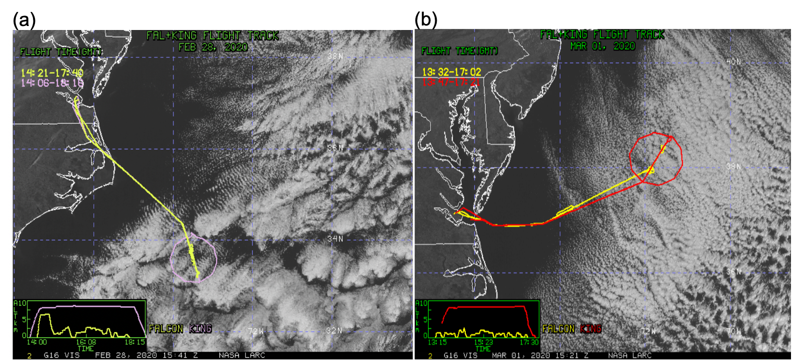
Figure 1 shows flight tracks of King Air and HU-25 Falcon and visible images from GOES-16 satellite during the two CAO process-study cases over the WNAO region on 28 February 2020 and 1 March 2020, corresponding to Research Flight $\#10$ and $\#13$ (hereafter RF10 and RF13), respectively. 11 dropsondes (model Vaisala NRD41) were released from the King Air. Each of them provided vertical profiles of air pressure ${\rm p}$, temperature $T$, relative humidity RH, and horizontal velocities $u$ and $v$ with a vertical resolution of 5-10 m and a resolution (with associated uncertainty) of 0.01 hPa ($\pm 0.5$ hPa), $0.01^{\circ}C$ ($\pm 0.2^{\circ}C$), $0.01\%$ ($\pm 0.3\%$), and $0.01\,{\rm m\,s}^{-1}$ ($\pm 0.5\,{\rm m\,s}^{-1}$) (National Center for Atmospheric Research 2021), respectively. The King Air flew in a circular pattern with a diameter of about $152\,{\rm km}$ to cover the largest enclosed area for dropsonde measurements and to avoid sharp turns. Such a flight pattern for the dropsonde measurements was first proposed by Lenschow et al. (1999). This strategy has been used in other campaigns to measure the large-scale divergence $D$, such as Elucidating the Role of Cloud–Circulation Coupling in Climate (Bony and Stevens 2019), Atlantic Tradewind Ocean-Atmosphere Mesoscale Interaction Campaign (Quinn et al. 2021), and Next-Generation Aircraft Remote Sensing for Validation (NARVAL2) airborne field campaign (Stevens et al. 2019). Dropsondes were released at a height of about 8 km. We interpolate the measured data evenly with a vertical spacing of 10 m for further analysis. Two contrasting CAO cases were observed over the WNAO region on February 28 (RF10, dropsonde-circle center at $33.66^{\circ}$N, $286.69^{\circ}$E) and March 1 (RF13, dropsonde-circle center at $38.01^{\circ}$N, $288.36^{\circ}$E) as shown in Figure 3. Table 1 summarizes the start/end time of dropsonde measurements, the location, $10$-m wind speed $U_{10\rm m}$, $q_{v,\rm{10m}}$, $T_{\rm{10m}}$, and ERA5 SST at the center of dropsonde circle for the February 28 and March 1 cases, respectively.

Table 1: This table lists the start-end time of dropsonde measurements, the location, $10$-m wind speed $U_{10\rm m}$, $q_{v,\rm{10m}}$, and $T_{\rm{10m}}$ at the center of dropsonde circle for the 28 February 2020 and 1 March 2020 cases. The corresponding SST from ERA5 reanalysis is also documented.

Case	Start-end times (UTC)	Lat (∘)	Lon (∘)	$U_{10\rm{m}}\,(\rm{m\,s}^{-1})$	$q_{v,10\rm{m}}$ ($\rm{g\,kg}^{-1}$)	$T_{10\rm{m}}\,(K)$	SST ($K$)
							MW-IR	ERA5
0228	1540-1645	33.66	286.69	5.94	4.64	286.75	293.25	293.60
0301	1451-1547	38.01	288.36	11.74	2.79	275.71	286.84	286.88

Dropsonde measurements are used to characterize the meteorological conditions and derive large-scale divergence and surface heat fluxes for both cases. Cloud droplets and ice crystals were observed for both cases. The mean number concentration of cloud droplets obtained from Fast Cloud Droplet Probe (FCDP, equipped on HU-25 Falcon) measurement (Taylor et al. 2019; Knop et al. 2021) is about $\langle N_{c}\rangle=650\,{\rm cm}^{-3}$ for the February 28 case and $\langle N_{c}\rangle=450\,{\rm cm}^{-3}$ for the March 1 case. These values are acquired by averaging in-cloud FCDP measurement with a lower cutoff of liquid water path of $0.02\,{\rm g\,kg}^{-1}$ and effective diameter of $3.5\,\mu{\rm m}$ (FCDP covers a diameter range of 3.0 to 50.0 $\mu{\rm m}$). There were also detailed measurements of aerosol particles including mass and number concentration, composition, size distribution, hygroscopicity, and optical properties. Given the focus of this study, we only use the mean cloud drop number in our LES sensitivity simulations on meteorological conditions and large-scale forcings. Liquid water path is retrieved from Research Scanning Polarimeter (RSP) (Alexandrov et al. 2012, 2018). Given the instantaneous field of view of 14 mrad, typical cloud tops (about 2 km), and a flight altitude of the King Air during ACTIVATE ($8\sim 9$ km), the nadir pixel size of the RSP is approximately 100 m. To compare with the LES with a 300 m horizontal grid spacing, we average the RSP sampling every 3 s, given that the moving speed of King Air is about $100\,\rm{m\,s}^{-1}$. Fast in-situ 3-D wind measurements were performed with an uncertainty of $5\%$ and a sampling frequency of 20 Hz. The static air temperature was measured with an uncertainty of $5\%$ and a sampling frequency of 1 Hz. The water vapor volume mixing ratio in ppmv was measured by Diode Laser Hygrometer with an uncertainty of $5\%$ and a sampling frequency of 1 Hz.

2.2 ERA5 and MERRA-2 reanalysis data

The ERA5 reanalysis data are generated using the fifth generation of European Centre for Medium-Range Weather Forecasts’s Integrated Forecast System (Hersbach et al. 2020). We use the ERA5 hourly data at a horizontal resolution of 31 km. For three-dimensional fields, there are 137 model levels up to a height of 80 km. Since ERA5 only provide $\bar{D}$ in datasets with specified pressure levels, we use pressure-level data for the comparison of $\bar{D}$ and the corresponding large-scale vertical velocity $w$. The ERA5 large-scale forcings for the LES are obtained at the model levels instead of the pressure levels because the model-level data have a finer vertical mesh-size and can better characterize the inversion layer. The ambient meteorological conditions for a given location during a CAO usually evolve quickly due to strong winds and large surface heat fluxes under winter mid-latitude weather disturbances. Since the measurement time window for the two CAO events is about one hour during the ACTIVATE field campaign, we are not able to use the measurements directly to drive the LES for many hours. We validate the ERA5 reanalysis data against the limited field measurements and then use the evolving forcing conditions from ERA5 reanalysis data to drive the LES.

The Modern-Era Retrospective analysis for Research and Applications version 2 (MERRA-2) (Global Modeling and Assimilation Office (2015) GMAO) is also used to compare with the ERA5 reanalysis and dropsonde measurements. The MERRA-2 reanalysis data are generated using the Goddard Earth Observation System version 5 (GEOS-5) with its Data Assimilation System version 5.12.4 (Gelaro et al. 2017). MERRA-2 has a horizontal resolution of $0.5^{\circ}\times 0.625^{\circ}$ with 72 model levels, from which the 3-hourly datasets at 42 pressure-levels are interpolated. It also provides 1-hourly two-dimensional datasets. We note that dropsonde measurements made during the ACTIVATE campaign have not been assimilated in either the ERA5 or MERRA-2 reanalysis used in this study. This allows us to validate meteorological states from LES and the reanalysis against the dropsonde measurements.

2.3 Satellite measurements

We use daily sea surface temperature (SST) retrieved from microwave and infrared based satellite measurements (MW-IR SST) produced by Remote Sensing Systems (National Centers for Environmental Information 2008). The SST product has a horizontal grid spacing of 9 km. This resolution is 3 times higher than the SST from ERA5 reanalysis data.

2.4 LES numerical experiment setup

We use the Weather Research and Forecasting (WRF) model (Skamarock et al. 2019) in the idealized LES mode (WRF-LES) (Wang and Feingold 2009) to simulate the two CAO cases and test the sensitivities of the marine BL and clouds to large-scale forcing and heat fluxes. Doubly periodic boundary conditions are employed in horizontal directions. The horizontal resolution is set to $dx=dy=300\,\rm{m}$ with 200 lateral grid cells, which results in a horizontal domain size of $L_{x}=L_{y}=60\,\rm{km}$. The domain height is $z_{\rm top}=7\,\rm{km}$ with 153 vertical $\eta$-layers ($\eta=(p-p_{\rm T})/(p_{\rm S}-p_{\rm T})$ with $p_{\rm S}$ and $p_{\rm T}$ the pressure at the bottom and top of the model domain, respectively), which results in a vertical mesh-size of about $33\,\rm{m}$ in the boundary layer. The horizontal resolution of 300 m is quite coarse for LES but it has proven to be able to simulate the formation and evolution of cloud cellular structures in marine stratocumulus (Wang and Feingold 2009). The periodic boundary condition in horizontal directions is ideal for isolating main governing factors for cloud processes and has been widely used for LES with lateral domain size even larger than $60\,\rm{km}$ (Seifert et al. 2015; Bretherton and Blossey 2017). The time step is set to $\Delta t=3\,{\rm s}$ in all simulations. Simulations are initiated at 06:00 UTC to allow sufficient model spin-up time before the WRF-LES results are evaluated against measurements taken during 16:00-17:00 UTC on February 28 and 15:00-16:00 UTC on March 1.

The two-moment Morrison cloud microphysics scheme (Morrison et al. 2009) is used. In this part of the study, a constant number concentration of cloud droplets derived from in-situ measurements during the ACTIVATE campaign is prescribed in the Morrison scheme to stay focused on cloud-meteorology interactions. Both shortwave and longwave radiative schemes are originally from the NCAR Community Atmosphere Model (CAM 3.0), which were used in previous WRF-LES studies, such as Wang et al. (2009) and Wang and Feingold (2009). Surface heat fluxes and SST are all prescribed in the model as the boundary conditions at the sea surface.

LES with horizontally uniform initial conditions and periodic boundary conditions cannot predict changes in atmospheric state at scales larger than its domain size. This is particularly true for rapidly evolving CAOs, with a baroclinic structure and the resulting vertical wind-profiles that cannot be properly simulated by LES (Gryschka et al. 2014). To circumvent this problem, we apply relaxation to horizontal wind components $u$ and $v$ and advective tendencies to potential temperature $\theta$ and water vapor mixing ratio $q_{v}$ as forcing terms in the prognostic equations. We adopt the same large-scale forcing and relaxation schemes as in Endo et al. (2015). To derive the large-scale forcings, we simplify the governing equation of $\theta$ and $q_{v}$ by removing sink and source terms as,

$$\frac{\partial\theta}{\partial t}=-{\bm{u}}\cdot{\bm{\nabla}}\theta=-u\frac{\partial\theta}{\partial x}-v\frac{\partial\theta}{\partial y}-w\frac{\partial\theta}{\partial z},$$ (1)

$$\frac{\partial q_{v}}{\partial t}=-{\bm{u}}\cdot{\bm{\nabla}}q_{v}=-u\frac{\partial q_{v}}{\partial x}-v\frac{\partial q_{v}}{\partial y}-w\frac{\partial q_{v}}{\partial z}.$$ (2)

Applying Reynolds decomposition to Equations (1) and (2) and ignoring the perturbation terms $\overline{{\bm{u}}^{\prime}\cdot{\bm{\nabla}}\theta^{\prime}}$ and $\overline{{\bm{u}}^{\prime}\cdot{\bm{\nabla}}q_{v}^{\prime}}$, we obtain temporal tendencies at large scales,

$$\frac{\partial\bar{\theta}}{\partial t}=\left[-\bar{u}\frac{\partial\bar{\theta}}{\partial x}-\bar{v}\frac{\partial\bar{\theta}}{\partial y}-\bar{w}\frac{\partial\bar{\theta}}{\partial z}\right]_{\rm{ERA5}},$$ (3)

and

$$\frac{\partial\bar{q}_{v}}{\partial t}=\left[-\bar{u}\frac{\partial\bar{q}_{v}}{\partial x}-\bar{v}\frac{\partial\bar{q}_{v}}{\partial y}-\bar{w}\frac{\partial\bar{q}_{v}}{\partial z}\right]_{\rm{ERA5}},$$ (4)

where the overbar denotes a large-scale mean. The large-scale horizontal advective tendencies of $\bar{\theta}$ and $\bar{q}_{v}$ are given by the first two terms of r.h.s of Equation (3) and Equation (4), respectively. The third term in the r.h.s of Equation (3) and Equation (4) represents the large-scale vertical advective tendencies. These large-scale advective tendencies are obtained from the hourly ERA5 reanalysis data and applied to each grid cell. Ignoring the perturbation terms $\overline{{\bm{u}}^{\prime}\cdot{\bm{\nabla}}\theta^{\prime}}$ and $\overline{{\bm{u}}^{\prime}\cdot{\bm{\nabla}}q_{v}^{\prime}}$ is for the practical reason that ERA5 reanalysis data do not resolve intermediate scales for our LES due to the relatively coarse mesh size of 31 km. In addition, such a forcing scheme was also adopted in previous studies, such as Siebesma and Cuijpers (1995); Endo et al. (2015). van Laar et al. (2019) took the contribution of intermediate scales into the large-scale forcing using $0.1^{\circ}\times 0.1^{\circ}$ mesh-sized forcing data. However, in the present study, we aim to clearly define the scales to be included as the large-scale contribution. The horizontal wind components $u$ and $v$ are applied with a relaxation strategy (i.e., nudging LES domain-average winds to a reference state), as also used in previous LES studies (Wang and McFarquhar 2008; Endo et al. 2015), defined by

$$\left.\frac{\partial u}{\partial t}\right|_{\rm R}=\frac{u_{\rm ERA5}-\langle u\rangle}{\tau},$$ (5)

$$\left.\frac{\partial v}{\partial t}\right|_{\rm R}=\frac{v_{\rm ERA5}-\langle v\rangle}{\tau},$$ (6)

where $\langle\rangle$ denotes average over the domain of WRF-LES, $\tau$ is the relaxation time scale, which is set to be 1 hour in this study. The subscript “R” denotes the relaxation adjustment to the horizontal wind components. The grid-scale wind is determined by Equations (5) and (6) and pressure gradients as the Coriolis force is set to zero in our LES. Overall, the large-scale forcing applied to LES is homogeneous horizontally.

We acknowledge that applying relaxation of wind to WRF-LES lacks physical judgment as also addressed in Endo et al. (2015). However, LES of horizontal winds with relaxation adjustments are found to be comparable with the reanalysis and observational data. This is not new and has been used in the single column model (Randall and Cripe 1999) and many LES works (Neggers et al. 2012; Heinze et al. 2017) in the meteorology community. Even though the simulation domain is stationary and a horizontal periodic boundary condition is used, the WRF-LES is set to take the cold air advection within CAO into account through the large-scale advective tendencies and wind relaxation described by Equations (3) and (4) and Equations (5) and (6), respectively.

We also test the sensitivities of WRF-LES results to prescribed surface heat fluxes obtained from ERA5 reanalysis data. Table 2 lists parameters examined in the sensitivity tests.

Table 2: List of WRF-LES with different forcings. $\rm{SHF(t)_{I}}$ and $\rm{LHF(t)_{I}}$ denote sensible and latent heat fluxes calculated interactively in WRF-LES.

Simulation	$\frac{\partial\bar{\theta}}{\partial t}$ $\&$ $\frac{\partial\bar{q}_{v}}{\partial t}$	$u\&v$ relaxation	SHF ($\rm{W\,m}^{-2}$)	LHF ($\rm{W\,m}^{-2}$)	$\bar{D}$	$N_{c}$ [$\rm{cm}^{-3}$]	dx (m)
0228A	Yes	Yes	79.91	305.02	Yes	650	300
0228B	No	Yes	79.91	305.02	Yes	650	300
0228C	Yes	No	79.91	305.02	Yes	650	300
0228D	No	No	79.91	305.02	Yes	650	300
0228E	Yes	Yes	SHF(t)	LHF(t)	Yes	650	300
0228F	Yes	Yes	$\rm{SHF(t)_{I}}$	$\rm{LHF(t)_{I}}$	Yes	650	300
0228G	Yes	Yes	SHF(t)	LHF(t)	Yes	650	100
0301A	Yes	Yes	231.76	382.18	Yes	450	300
0301B	Yes	Yes	231.76	LHF(t)	Yes	450	300
0301C	Yes	Yes	SHF(t)	382.18	Yes	450	300
0301D	Yes	Yes	231.76	382.18	No	450	300
0301E	Yes	Yes	SHF(t)	LHF(t)	Yes	450	300
0301F	Yes	Yes	$\rm{SHF(t)_{I}}$	$\rm{LHF(t)_{I}}$	Yes	450	300
0301G	Yes	Yes	SHF(t)	LHF(t)	Yes	450	100

3 Meteorological conditions and forcings for the two cases

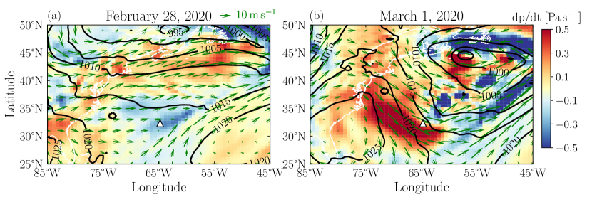
Figure 2 shows synoptic weather maps at 18:00 UTC from MERRA-2 for the February 28 and March 1 cases over the ACTIVATE measurement region. A low pressure system at the upper-left domain on February 28 moved to the southeast on March 1 with an anticyclone development along the coast. The Februray 28 case is featured by synoptic-scale ascending motion (negtitive omega velocity $\rm{dp/dt}$) and westerly winds over the sampling domain. The March 1 case features a subsidence region (positive omega velocity $\rm{dp/dt}$) east of the coastal anticyclone and dominant northwesterly winds west of $60^{\circ}$W.

Figure 2: Synoptic weather maps for the (a) February 28 and (b) March 1 cases. The colored contours, green arrows, and black contours represent MERRA-2 omega velocity $\rm dp/dt$ at 600 hPa (positive indicates downward), averaged winds ($\rm{m\,s^{-1}}$) at 900 hPa, and sea level pressure at 18:00 UTC over the ACTIVATE measurement region, respectively. Solid black circles represent the location of dropsondes. Triangles represent the location of Bermuda Island. The white lines indicate coastlines. The length of green arrows is proportional to the magnitude of wind speeds. The benchmark length represents $10\,\rm{m\,s^{-1}}$ wind speeds. The instantaneous fields at 18:00 UTC is plotted to match the time of MERRA-2 and dropsonde measurements.

3.1 Dropsonde measurements and derived divergence

Figure 3 shows the location of individual dropsondes and the center of dropsonde circle on an ERA5 SST map for both cases. The nearest ERA5 grid points to the dropsondes are also shown in gray open symbols which are used to obtain the SST for the corresponding dropsondes. Clearly, the SST is much warmer over the circle on February 28 than March 1.

Figure 3: Location of dropsondes for the (a): February 28 and (b): March 1 cases. Black open symbols are the location of dropsondes at the surface and the gray ones are mapped locations from the ERA5 reanalysis data. Solid dots represent the center of the dropsonde circle. The contour map shows ERA5 SST in the measurement region. The black star represent the location of Hampton, VA on this map. The red curve shows the flight path. The white lines and gray area indicate coastlines and the land, respectively.

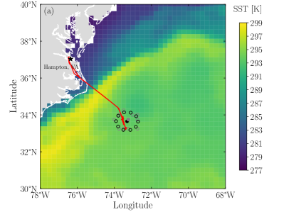
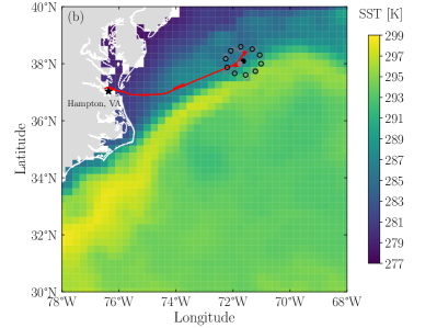
Figure 4 shows the vertical profiles of RH, $q_{v}$, $\theta$, $u$, and $v$ from dropsonde measurements for the two cases. The February 28 case (RF10) is characterized by a deeper boundary layer with a depth of about $2.8\,{\rm km}$ and a drier free troposphere compared to the March 1 case (RF13). Individual RH and $q_{v}$ profiles show more fluctuations from the mean in the free troposphere on March 1 than the February 28 case. The boundary layer for the March 1 case is shallower. The magnitude of $u$ and $v$ increases rapidly with height above the boundary layer, which is more profound on February 28, showing a strong wind shear. The meteorological states evolve substantially during the one-hour sampling time period of both cases, as indicated by the contrast between the first dropsonde (blue curve) and the last one (red curve) that were released roughly at the same location. The boundary layer became deeper (shallower) with time on February 28 (March 1).

Figure 4: Profiles from dropsonde measurements for the February 28 (upper panel) and March 1 cases (lower panel). The gray lines represent vertical profiles measured from 11 dropsondes and the thick black lines represent the corresponding mean profile. The blue and red curves represent the first and last dropsonde, respectively, released at about the same location but one hour apart.

The vertical velocity of airflow regulates the atmospheric water distribution but is difficult to measure (Bony and Stevens 2019). The continuity equation of nearly incompressible airflow with velocity $\bm{u}=\bm{u}(u,v,w)$ is given by

$${\bm{\nabla}}\cdot{\bm{u}}=\frac{\partial u}{\partial x}+\frac{\partial v}{\partial y}+\frac{\partial w}{\partial z}=0.$$ (7)

According to Equation (7), the vertical velocity $w$ can be expressed as

$$w(z)=-\int_{0}^{z}\left(\frac{\partial u}{\partial x}+\frac{\partial v}{\partial y}\right){\rm d}z^{\prime}.$$ (8)

Divergence is defined as

$$D=\frac{\partial u}{\partial x}+\frac{\partial v}{\partial y}.$$ (9)

Thus, Equation (9) can be written as

$$w(z)=-\int_{0}^{z}D{\rm d}z^{\prime}.$$ (10)

Therefore, $w$ can be indirectly obtained from the measured horizontal wind components. In the atmospheric boundary layer, motion of airflow is conventionally decomposed to large and small scales. By applying Reynolds decomposition to Equation (7), we obtain the large-scale divergence,

$$\bar{D}=\frac{\partial\bar{u}}{\partial x}+\frac{\partial\bar{v}}{\partial y}.$$ (11)

We follow the procedure described by Lenschow et al. (2007) to calculate the divergence from dropsonde measurements, details of which are given in Appendix A. Since we use the linear regression method to estimate $\bar{D}$, the standard error $\sigma_{\epsilon}$ can be estimated. The large-scale divergence $\bar{D}$ enters the third term in the r.h.s of Equation (3) and Equation (4) through Equation (10). Thus the effect of $\bar{D}$ is taken into account via vertical motion, $w$, in the vertical component of the advective tendency.

We compare $\bar{D}$ estimated from the dropsonde measurements with the one obtained from ERA5 reanalysis data for both cases as shown in Figure 5. ERA5-$\bar{D}$ profile (red curve) averaged between 16:00 UTC and 17:00 UTC (two vertical profiles) at the dropsonde center is able to capture the sign of $\bar{D}$ vertical-structure measured by dropsonde (black curve) for the February 28 case (Figure 5(a)) within 1 km above the surface. However, it differs from the dropsonde measurements in both signs and magnitude above 1 km, which requires further investigation. More interestingly, ERA5-$\bar{D}$ profile evolves from convergence to divergence within the boundary layer from 16:00 UTC (blue curve) to 17:00 UTC (cyan curve). We also examine the ERA5 $\bar{D}$ averaged between 16:00 UTC and 17:00 UTC at the location of each dropsonde as shown by coral-colored dashed lines in Figure 5, which exhibits large spatial fluctuations. This demonstrates strong spatial inhomogeneity in large-scale vertical motions over this area on February 28, as also indicated by the sensitivity of $\bar{D}$ to different dropsonde subsets as shown in Figure 20. The amplitude of the mean and largest value of dropsonde-$\bar{D}$ for the February 28 case is $\langle|\bar{D}|\rangle=1.38\times 10^{-5}\,{\rm s}^{-1}$ and $|\bar{D}|_{\rm max}=4.06\times 10^{-5}\,{\rm s}^{-1}$, respectively. For the March 1, they are $\langle|\bar{D}|\rangle=2.99\times 10^{-5}\,{\rm s}^{-1}$ and $|\bar{D}|_{\rm max}=7.09\times 10^{-5}\,{\rm s}^{-1}$. These values are about one order of magnitude larger than the ones from non-CAO marine BL cloud regimes. The mean value of $\bar{D}$ inferred from the ensemble of radiosondes during the Atlantic Trade-Wind Experiment (Augstein et al. 1973) and the Barbados Oceanographic and Meteorological Experiment (Holland and Rasmusson 1973) is about $10^{-6}\,{\rm s}^{-1}$. Similar values were used in the case studies during the VAMOS Ocean-Cloud-Atmosphere-Land Study (Rahn and Garreaud 2010; Wang et al. 2010) and Second Dynamics and Chemistry of Marine Stratocumulus field study (DYCOMS II) field campaign (Wang and Feingold 2009). $\bar{D}$ estimated during the NARVAL2 is about $10^{-5}\,\rm{s^{-1}}$ (Bony and Stevens 2019).

Figure 5: Comparison of $\bar{D}$ profiles estimated from dropsonde measurements with the one from ERA5 reanalysis data for the (a): February 28 and (b): March 1 cases. Black dotted lines represent $\bar{D}$ estimated from 10 dropsondes with $\pm\sigma_{\epsilon}$ uncertainty (gray shaded area). Blue lines represent ERA5-$\bar{D}$ profiles at 16:00 UTC for the February 28 and 17:00 UTC for the March 1 cases at the center of dropsondes. Cyan lines represent ERA5-$\bar{D}$ profiles at 17:00 UTC for the February 28 and 16:00 UTC for the March 1 cases at the center of dropsondes. Red solid-dotted lines represent $\bar{D}$ from ERA5 reanalysis data averaged during the measurement time (between blue lines and cyan lines). The dashed coral-colored lines represent ERA5 reanalysis data at the location of individual dropsondes averaged during the measurement time for each case.

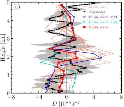
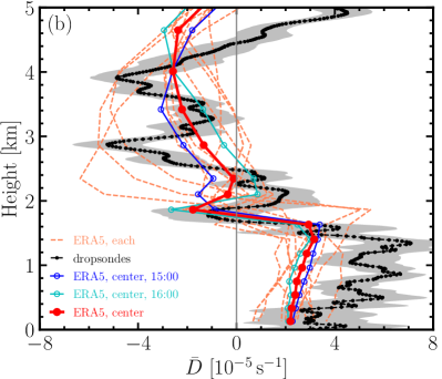
Figure 5(b) shows the same comparison but with the dropsonde measurements conducted on March 1. In this case, $\bar{D}$ obtained from ERA5 reanalysis data (red solid-dotted line) at the center of dropsonde circle is able to capture the general vertical structure of $\bar{D}$ estimated from dropsonde measurements. Similar to the February 28 case, there is a strong spatiotemporal variation in the ERA5 $\bar{D}$.

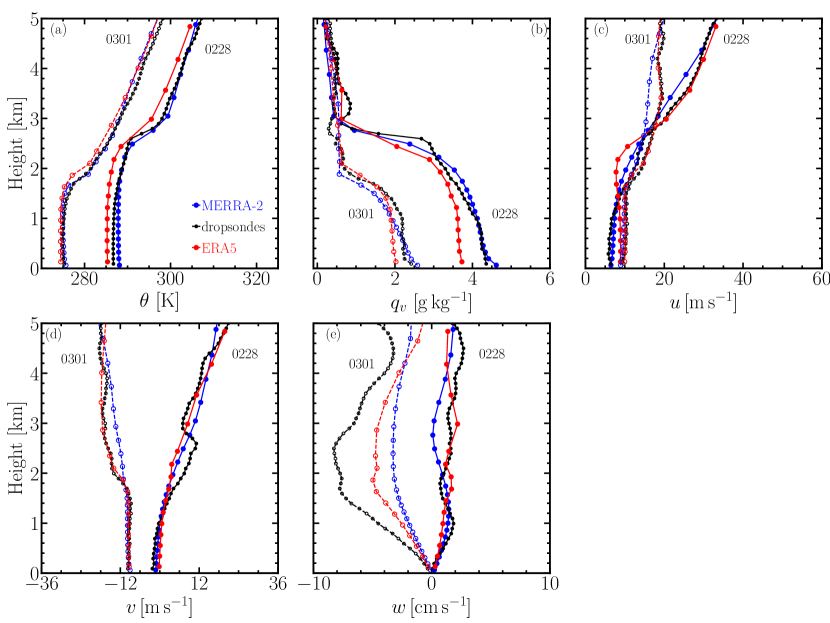
We further compare the large-scale vertical velocity $w$ (subsidence) with MERRA-2 reanalysis data as shown in Figure 6(e) for both cases. For the February 28 case, the $w$ profile from MERRA-2 is averaged between 15:00 UTC and 18:00 UTC and the one from ERA5 is averaged between 16:00 UTC and 17:00 UTC to better match the dropsonde sampling time. Both the ERA5 and MERRA-2 can reasonably capture the vertical profile of $w$ when compared with dropsonde measurements for this case. For the March 1 case, the $w$ profile from MERRA-2 reanalysis data at 15:00 UTC is used to compare with dropsonde measurements while the one from ERA5 reanalysis data is averaged between 15:00 UTC and 16:00 UTC. The ERA5 reanalysis data agree with the dropsonde measurements in the sign but underestimate the magnitude. The MERRA-2 does not capture the structure and magnitude of the vertical profile of $w$ well. Comparison of $\theta$, $q_{v}$, $u$, and $v$ profiles is also shown in Figure 6(a)–(d). MERRA-2 shows a slightly warmer boundary layer for the February 28 case while the ERA5 shows a colder one. Both MERRA-2 and ERA5 data capture the $\theta$ profile well for the March 1 case. ERA5 yields a drier ($q_{v}$ profiles) boundary layer while MERRA-2 capture the $q_{v}$ well compared to the dropsonde measurements for both cases. The $u$ and $v$ profiles within the boundary layer are represented well by MERRA-2 and ERA5 data for both cases, given the large spread among the individual dropsondes for the circled area (see Figure 4). The ERA5 captures those profiles above the boundary layer better than the MERRA-2. Overall, comparing to MERRA-2, ERA5 profiles are more consistent with the dropsonde measurements, as also shown in Chellappan et al. (2021) for the broader WNAO region.

Since we aim to use the divergence as part of the large-scale forcings to drive WRF-LES, the agreement of $\bar{D}$ (and the corresponding $w$) from ERA5 with the estimates from dropsondes for the March 1 case affords confidence to use the hourly ERA5 divergence to test the sensitivity of WRF-LES to time-varying large-scale forcings.

Figure 6: Comparison among dropsonde measurements (black curves), ERA5 (red curves), and MERRA-2 (blue curves) at the dropsonde center for both cases. Solid symbols represent the February 28 case (ERA5 data averaged between 16:00 and 17:00 UTC and MERRA-2 averaged between 15:00 and 18:00 UTC) and the open circles mark the March 1 case (ERA5 averaged between 15:00 and 16:00 UTC and MERRA-2 at 15:00 UTC). Large-scale vertical velocity $w$ from ERA5 corresponds to ERA5-$\bar{D}$ in Figure 5.

3.2 Surface heat fluxes

Turbulent sensible and latent heat fluxes at the surface are important flux boundary conditions to drive LES of boundary layer clouds. They are responsible for the heat and moisture exchange between the ocean and atmosphere. Surface heat fluxes are challenging to measure and estimate due to the nonlinear processes involved. Therefore the so-called bulk aerodynamics parameterization has been used to estimate surface heat fluxes. Bulk aerodynamics algorithms parameterize the turbulence instability as well as the roughness length of the wind speed, temperature and the water vapor mixing ratio (Zeng et al. 1998). The surface sensible heat flux (SHF) and latent heat flux (LHF) are given by (Smith 1988)

$${\rm SHF}=C_{T}\rho c_{\rm p}U(T_{\rm s}-\theta),$$ (12)

$${\rm LHF}=C_{E}L_{v}\rho U(q_{\rm s}-q_{v}),$$ (13)

where $\rho$ is the air mass density, $c_{\rm p}$ is the specific heat of air, $U$ is the mean wind speed at a particular reference height, $T_{\rm s}$ is the SST, $\theta$ is the potential temperature at the reference height, $q_{\rm s}$ is the saturated water vapor mixing ratio, $q_{v}$ is the water vapor mixing ratio, and $L_{v}$ is the latent heat of evaporation. The sensible heat flux coefficient $C_{T}$ and evaporation coefficient $C_{E}$ are determined by the empirical Monin–Obukhov (MO) similarity theory. In this study, we adopt the bulk aerodynamics algorithms developed by Zeng et al. (1998) to calculate heat fluxes for comparison between ERA5 and dropsonde measurements, which we refer to as “Z98” hereafter. The Z98 algorithm calculates $C_{T}$ and $C_{E}$ based on instability analysis. Equation (12) and Equation (13) are used to calculate SHF and LHF after $C_{T}$ and $C_{E}$ are obtained. The input parameters of the Z98 algorithm are $T_{\rm s}$, 10-m (reference height) wind speed $U_{10\rm m}$, temperature $T_{10\rm m}$ (to calculate $\theta_{10\rm m}$), and the water vapor mixing ratio $q_{v,10\rm m}$.

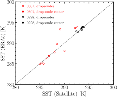
To derive the surface heat fluxes using dropsonde measurements and evaluate ERA5 reanalysis data, we first compare the ERA5 SST to satellite measurement for the two cases as a quality check. As shown in Figure 7, for both 28 February 2020 (black symbols) and 1 March 2020 cases (red symbols), SST from ERA5 and the satellite measurement matches well at the center of dropsonde circle. At the location of individual dropsondes the agreement is reasonable on February 28 while several points on March 1 are quite off, which is likely because of the location mismatch due to the resolution difference and sampling area being near strong SST gradients (shown in Figure 3). The Normalized Root-Mean-Square Error (NRMSE) is $0.1\%$ for the February 28 case and is $0.6\%$ for the March 1 case. This comparison suggests that the SST from ERA5 can also be used as the initial input for our WRF-LES. ERA5 has assimilated the Operational Sea Surface Temperature and Sea Ice Analysis (OSTIA) system for hourly SST starting from 2007 (Hirahara et al. 2016). The OSTIA assimilated the MW-IR measurements. Thus, the agreement between ERA5 and the satellite retrievals is expected.

Figure 7: Comparison of SST from satellite retrievals and ERA5 reanalysis data for both February 28 (black) and March 1 (red) cases . Open symbols represent SST at the position of each dropsonde. The two solid dots represent SST at the center of dropsonde circles.

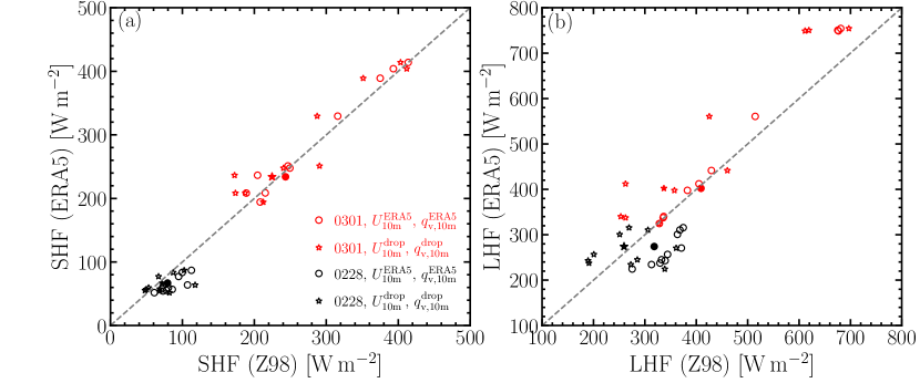
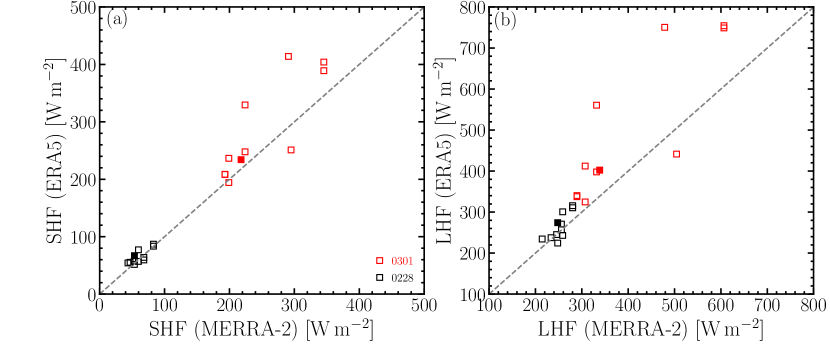
Next, we compare surface heat fluxes directly obtained from ERA5 reanalysis data and the ones estimated from ACTIVATE measurements. Since the SST obtained from ERA5 agrees with the satellite measurement, we try to examine if the ERA5 heat-fluxes can be reproduced from ERA5 SST and dropsonde measurements. First, we use the Z98 algorithm to calculate heat fluxes based on $T_{\rm s}^{\rm ERA5}$, $U_{\rm 10m}^{\rm ERA5}$, $q_{v,{\rm 10m}}^{\rm ERA5}$ from ERA5 and $T_{\rm 10m}^{\rm drop}$ from dropsonde. Figure 8(a) shows the comparison between the estimated SHF and the ERA5 reanalysis data (red and black circles). The corresponding NRMSE is $5.1\%$ and is $36.4\%$ for the March 1 and February 28 case, respectively. The comparison of LHF is shown in Figure 8(b) with NRMSE of $8.5\%$ and $30.0\%$ for the March 1 (red circles) and February 28 case (black circles), respectively. These demonstrate a good agreement between the estimated heat fluxes and the ERA5 reanalysis data on March 1 case, given the large spread within the dropsonde circle. The agreement is particularly good at the circle center (solid symbols). This suggests that the Z98 algorithm can be used to calculate heat fluxes and the use of $T_{\rm 10m}^{\rm drop}$ is justified in this study. It is evident that SHF and LHF calculated using Z98 are underestimated compared to ERA5 for the February 28 case. This is because ERA5-$\theta$ is smaller than the dropsonde-$\theta$ within the boundary layers as shown in Figure 6(a). We then use $U_{\rm 10m}^{\rm drop}$ and $q_{v,{\rm 10m}}^{\rm drop}$ obtained from dropsonde measuremens to estimate the fluxes (stars in Figure 8), which yields a NRMSE value of $11.5\%$ for SHF and $19.3\%$ for LHF for the March 1 case, further indicating that ERA5 gives a good estimate of turbulent heat fluxes for the March 1 case. For the February 28 case, NRMSE of SHF and LHF calculated using $U_{\rm 10m}^{\rm drop}$ and $q_{v,{\rm 10m}}^{\rm drop}$ are $33.2\%$ and $23.1\%$, respectively. This underestimation is because that $q_{v}$ from ERA5 is smaller than the one from dropsonde measurements within the boundary layer as shown in Figure 6(b). We also compare heat fluxes between the ERA5 and MERRA-2 reanalysis data. Both SHF and LHF agree well between MERRA-2 and ERA5 for the February 28 case. However, MERRA-2 underestimates SHF and LHF compared to ERA5 for the March 1 case (see appendix B).

Overall, by adopting $T_{\rm s}^{\rm ERA5}$, $U_{\rm 10m}$, $q_{\rm v,10m}$, and $T_{\rm 10m}^{\rm drop}$ from dropsonde measurements to estimate heat fluxes using Z98 algorithm, we are able to evaluate the heat fluxes from ERA5. The time-varying ERA5 heat fluxes are then used in the WRF-LES sensitivity tests. The method of using dropsonde measurements to estimate surface heat fluxes was also adopted for studying the tropical cyclones (Powell et al. 2003; Holthuijsen et al. 2012; Richter et al. 2016). These studies show that the accuracy of estimated coefficients based on MO similarity theory decreases with increasing wind speed. In the present study, the wind speed is orders of magnitude smaller than that of tropical cyclones, which ensures the accuracy of using dropsonde measurement to estimate surface heat fluxes.

Figure 8: Comparison between the estimated heat fluxes and the one from ERA5 reanalysis data at 16:00 UTC for the February 28 case (black symbols) and 15:00 UTC for the March 1 case (red symbols). $T_{\rm s}^{\rm ERA5}$ is adopted for the calculation. Open symbols represent $T_{\rm s}^{\rm ERA5}$ at the position of individual dropsondes and solid symbols represent the center of the dropsonde circle. Two sets of input variables are adopted to calculate the surface heat fluxes: $U_{10\rm m}^{\rm ERA5}$ and $q_{v,10\rm m}^{\rm ERA5}$ (circles) and $U_{10\rm m}^{\rm drop}$ and $q_{v,10\rm m}^{\rm drop}$ (stars).

4 WRF-LES sensitivities to large-scale forcings and contrast between the two CAO cases

4.1 Sensitivities to large-scale advective tendencies and relaxation

In this section, we investigate how to better represent time-varying meteorological states in idealized WRF-LES applying either advective tendencies to $\theta$ and $q_{v}$, relaxation to $u$ and $v$, or both. Simulations are driven by constant surface fluxes ${\rm SHF}(t_{0})$ and ${\rm LHF}(t_{0})$. Here $t_{0}$ denotes the starting time of simulations. Since we have shown in the previous section that ERA5 reanalysis data agree well with the dropsonde measurements during the sampling time periods of the two CAO cases, we adopt hourly $\theta$, $q_{v}$, $u$, and $v$ vertical profiles from ERA5 reanalysis data and derive the corresponding vertical profiles of advective tendencies and relaxation adjustments. The hourly meteorological states simulated in WRF-LES are then compared to ERA5 reanalysis data that are partly validated against dropsonde measurements.

Figure 9 shows the hourly (rainbow-colored lines) input meteorological forcing being obtained from ERA5 reanalysis data for the WRF-LES simulations. The evolution of vertical profiles are averaged over a $2^{\circ}\times 2^{\circ}$ area centered at the middle of the dropsonde circle of each case. This selected area sufficiently covers the dropsonde circle. Vertical profiles of $\theta$, $q_{v}$, $u$, $v$, and $w$ obtained from ERA5 reanalysis data averaged during the measurement time (black solid lines) agree reasonably well with the dropsonde measurements (gray dashed lines) for the February 28 case (upper row) and for the March 1 case (lower row). Vertical profiles of advective tendencies of $\theta$ and $q_{v}$ (i.e., $\partial\bar{\theta}/\partial t$ and $\partial\bar{q}_{v}/\partial t$) are calculated from $\theta_{\rm ERA5}$ and $q_{v,\rm ERA5}$. Vertical profiles of $\theta_{\rm ERA5}$, $q_{v,\rm ERA5}$, $u_{\rm ERA5}$, and $v_{\rm ERA5}$ at 06:00 UTC are taken as the input sounding for WRF-LES when the simulation starts. We note that $w_{\rm ERA5}$ averaged over the $2^{\circ}\times 2^{\circ}$ area at 15:00 UTC differs slightly from the one at the dropsonde center shown by the red curve in Figure 6 as expected. This is because of the strong spatial variation of $\bar{D}$ as shown in Figure 5. We have tested the relaxation time scale $\tau$ of $u$ and $v$ for the February 28 case and found that WRF-LES with $\tau$=30 min, 1 h, and 3 h reveal almost identical vertical profiles and liquid water path (LWP). Therefore we adopt $\tau$=1 h for all the simulations as the ERA5 reanalysis data has a time resolution of one hour. The relaxation is applied to all vertical layers of the LES domain.

Figure 9: Hourly meteorological state and forcing profiles for the February 28 case (simulation 0228A, upper panel) and March 1 case (simulation 0301A, lower panel) from ERA5 reanalysis data averaged over a $2^{\circ}\times 2^{\circ}$ domain. The rainbow color scheme represents the time evolution (06:00-21:00 UTC): from purple to red. The averaged ERA5 reanalysis data over the measurement time period are marked by black lines, which are compared with the dropsonde measurements (dashed gray lines).

We first perform a simulation without applying advective tendencies of $\theta$ and $q_{v}$ and relaxation of $u$ and $v$ (simulation 0228D) for the February 28 case. It is shown by the blue curves in Figure 10 that such a configuration yields vertical profiles that have a large deviation from the ERA5 reanalysis data (cyan curves) and dropsonde measurements (grey curves). The $\theta$ profile from WRF-LES differs considerably from ERA5 above the boundary layer and the $q_{v}$ profile shows a more humid boundary layer than the ERA5 (the ratio of $q_{v}$ from “Both” to that from “ERA5” is 1.32 averaged within the boundary layer with a depth of 2.4 km during the measurement time). The $u$ and $v$ profiles from WRF-LES deviate from the ERA5 and dropsonde measurements. When $\partial\bar{\theta}/\partial t$ and $\partial\bar{q}_{v}/\partial t$ are applied (simulation 0228C), $\theta$ and $q_{v}$ profiles from WRF-LES agree well with the dropsonde measurements as shown by the red curves in Figure 10. However, $u$ and $v$ profiles still deviate from the ERA5 reanalysis data. We then only apply the $u$ and $v$ relaxation to the WRF-LES (simulation 0228B). As shown by the green curves of Figure 10, $u$ and $v$ profiles from WRF-LES are in good agreement with dropsonde measurements even though $\theta$ and $q_{v}$ profiles differ from the measurements. This naturally leads to the configuration of applying advective tendencies of $\theta$ and $q_{v}$ together with $u$ and $v$ relaxation to $u_{\rm ERA5}$ and $v_{\rm ERA5}$ (simulation 0228A). Such a configuration leads to vertical profiles ($\theta$, $q_{v}$, $u$, and $v$) that are comparable to ERA5 reanalysis data and dropsonde measurements as shown by the black curves of Figure 10. Therefore, this combined forcing and relaxation scheme is justified to simulate the two CAO cases. Evolution of the vertical profiles for simulations 0228A, 0228B, 0228C, and 0228D are shown in section D. As also shown in Figure 10, the magnitude and time evolution of cloud water simulated by WRF-LES are sensitive to the boundary layer meteorological conditions.

Figure 10: Domain-averaged vertical profiles for simulation 0228A (black curve), 0228B (green curve), 0228C (red curve), and 0228D (blue curve) with the corresponding input forcings shown in Figure 9 for the February 28 case during the measurement time listed in Table 1. The cyan curve represent profiles from the ERA5 reanalysis data averaged during the measurement time and the grey curve represent the ones from dropsonde measurements. Heat fluxes are from ERA5 reanalysis data: ${\rm SHF}(t_{0})=79.91\,\rm{W\,m}^{-2}$ and ${\rm LHF}(t_{0})=305.02\,\rm{W\,m}^{-2}$.

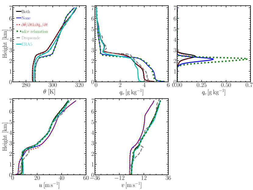
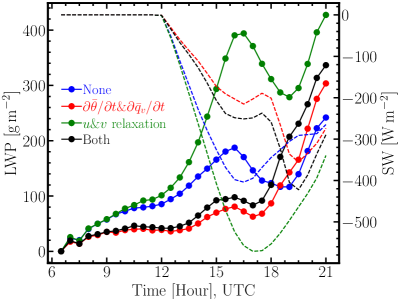
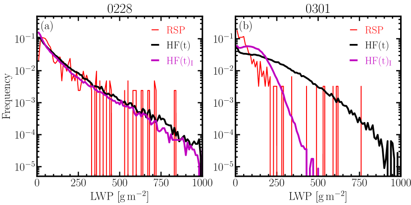
Applying $\partial\bar{\theta}/\partial t$ and $\partial\bar{q}_{v}/\partial t$ leads to a colder and less humid boundary layer (compare simulation 0228C and 0228D) but allows the boundary layer to grow higher. This results in a deeper cloud layer with a reduced amount of the liquid water content $q_{c}$, which is enhanced by a factor of two by applying $u$ and $v$ relaxation (compare simulation 0228B to 0228D). We then examine the time evolution of LWP. LWP peaks around 16:00 UTC and then starts to decrease as shown in Figure 11, which could be due to the solar heating. The short-wave (SW) cloud forcing at the top of atmosphere increases with increasing LWP at a fixed time as indicated by the dashed lines in Figure 11. To validate the simulated LWP, we compare it with the RSP retrievals during the ACTIVATE field campaign. As shown in Figure 12(a), the WRF-LES (shown as the black line, averaged over the measurement time) agrees reasonably well with the RSP measurement. This further illustrates that the WRF-LES is able to capture the cloud formation and evolution in this case study. We also tested the tendencies and relaxation forcing for the March 1 case, which yields the same conclusion as for the February 28 case. Figure 12(b) shows that the WRF-LES underestimates the frequency of lower LWP values (less than $100\,{\rm g\,m}^{-2}$) but overestimates the frequency between $200-400\,{\rm g\,m}^{-2}$ for the March 1 case.

Figure 11: Time series of domain-averaged LWP (liquid cloud and rain, solid symbols) and short-wave (SW) cloud forcing at the top of atmosphere (dashed lines) of simulations (blue:0228D, red:0228B, green:0228C, black:0228A) with different forcing options as shown in Figure 10.

Figure 12: Comparison of frequency distribution of LWP between RSP measurements and WRF-LES for (a): February 28 (0228E) and (b): March 1 (0301E) cases. ${\rm HF(t)_{I}}$ denotes heat fluxes calculated interactively (0228F and 0301F) from WRF-LES. The frequency for WRF-LES LWP is calculated from 3 snapshots (every 30 minutes) during the measurement time. Note that the boundary layer evolves as shown in the last row of Figure 27. LWP samples are binned into 100 bins with a uniform width of $10\,\rm{g\,m}^{-2}$. The minimum value of LWP from the RSP measurement ($2.4\,\rm{g\,m}^{-2}$ and $0.6\,\rm{g\,m}^{-2}$ for the February 28 and March 1 cases, respectively) is taken as a lower cutoff for the simulated LWP.

4.2 Sensitivities to large-scale divergence $\bar{D}$

We have shown that applying $\partial\bar{\theta}/\partial t$, $\partial\bar{q}_{v}/\partial t$, $u$ relaxation to $u_{\rm ERA5}$, and $v$ relaxation to $v_{\rm ERA5}$ is essential to reproduce the time evolution of meteorological states for the two CAO cases considered in this study. This configuration is adopted to further test the sensitivities of WRF-LES results to $\bar{D}$. We focus on the March 1 since it is more challenging to simulate due to the large surface heat fluxes.

We perform two WRF-LES with or without the large-scale vertical velocity as a forcing (third term on the r.h.s of Equations (3) and (4)) for the March 1 case. The forcing configuration for the baseline simulation 0301A is the same as simulation 0228A. To examine the impact of large-scale divergence separately, we conduct a simulation (0301D in Table 2) that excludes the forcing term related to $\bar{D}$ (vertical component of the advective tendencies) but keeps all other forcings the same as the baseline (0301A). As shown in Figure 13, the initial model spin-up time (06:00-08:00 UTC) is characterized by a sharp increase of LWP from 0 to about $200\,\rm{g\,m}^{-2}$ for the baseline simulation (blue). Without the time varying large-scale divergence (cyan), LWP and Ice Water Path (IWP) experience a larger increase compared to the baseline (blue) during the initial time steps because of the lack of subsidence that tends to suppress the growth of BL. LWP from simulation 0301D decreases and becomes smaller compared to the one from simulation 0301A. This is because IWP from 0301D are about 10 times more than the ones from 0301A. In the absence of $\bar{D}$, the updraft cooling is more profound. Thus, the ice formation is enhanced. The cyan curve in Figure 14 shows the deviation of vertical profiles of the simulation 0301D to 0301A averaged over the measurement time. As expected from a positive $w$, a much deeper boundary layer is developed in the simulation without subsidence. The moist air is mixed to over 3 km. This can be explained by the fact that the lack of divergence breaks the balance between the BL growth driven by surface fluxes and suppression due to subsidence. Figure 15 shows the contribution of horizontal and vertical advective tendencies to $\partial\theta/\partial t$ (upper row) and $\partial q_{v}/\partial t$ (lower row) for simulation 0301A and 0301D, respectively. When $\bar{D}=0$ (simulation 0301D), only horizontal advective tendencies contribute to $\partial\theta/\partial t$ by comparing the solid cyan curves in Figure 15(a)–(c). When $\bar{D}\neq 0$, it is evident that the vertical advective term ($\bar{D}$) dominates the temperature and humidity changes due to large-scale tendencies, especially near the inversion layer. The contribution from horizontal terms are small when comparing simulations 0301A and 0301D. The vertical profiles of $\partial\theta/\partial t$ and $\partial q_{v}/\partial t$ only evolve slightly from 15:00 to 16:00 UTC because $\bar{D}$ does not vary much for the March 1 case. Recall that for the February 28 case, $\bar{D}$ evolves from convergence to divergence from 16:00 to 17:00 UTC (Figure 5(a)). Consequently, the vertical profiles of $\partial\theta/\partial t$ and $\partial q_{v}/\partial t$ are nealry zero as shown in Figure 15. When comparing vertical profiles of $\partial\theta/\partial t$ and $\partial q_{v}/\partial t$ for the March 1 (blue lines) and February 28 (black lines) cases, we see that $\bar{D}$ has a more profound impact for the March 1 case.

Figure 13: Time series of domain-averaged (a): LWP (in-cloud liquid water and rain) and (b): IWP (ice, graupel, and snow) from WRF-LES (blue: 0301A, red: 0301B, green: 0301C, cyan: 0301D, black: 0301E) with different heat fluxes and large-scale divergence as indicated by the legends for the March 1 case. Heat fluxes are from ERA5 reanalysis data, the values of which are $\rm{SHF}(t_{0})=231.76\,\rm{W\,m}^{-2}$ and $\rm{LHF}(t_{0})=382.18\,\rm{W\,m}^{-2}$. Here $t_{0}$ denotes the starting time of the WRF-LES, which is 06:00 UTC.

Figure 14: Deviation of vertical profiles of simulation 0301B, 0301C, 0301E, and 0301D from the baseline simulation 0301A averaged over the measurement time (3 snapshots over 15:00 to 16:00 UTC).

Figure 15: Contributions of large-scale forcings to $\partial\theta/\partial t$ (upper row) and $\partial q_{v}/\partial t$ (lower row) for simulation 0301A (blue curves) and 0301D (cyan curves) at 15:00 UTC (solid lines) and 16:00 UTC (dashed lines). Black lines represent the ones for simulation 0228A at 16:00 UTC (solid line) and 17:00 UTC (dashed line). LS, LSHOR, and LSVER denote large-scale forcing due to total, horizontal, and vertical advective tendencies, respectively.

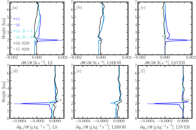
To conclude, $\bar{D}$ likely has a strong control on the time evolution of the boundary layer in WRF-LES of the two CAO events we explored here, especially for the March 1 case. Therefore, including a time-varying $\bar{D}$ profile to drive WRF-LES is necessary for simulating the fast-evolving CAO events over WNAO.

4.3 Sensitivities to surface heat fluxes

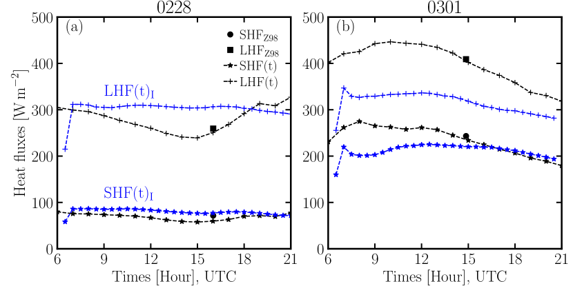
To test the sensitivities to surface fluxes, we perform another three WRF-LES simulations using the same forcing configuration as the baseline simulation 0301A but with temporally varying and spatially uniform surface heat fluxes for the March 1 case. The time series of such surface heat fluxes obtained from ERA5 reanalysis data at the center of dropsonde circle is shown as the black lines in Figure 16. As shown in Figure 13, when the WRF-LES is forced by ${\rm SHF}(t_{0})$ and ${\rm LHF}(t)$ (red curve), LWP evolves in the same pattern as the baseline but with larger values between 10:00-16:00 UTC. This is because ${\rm LHF}(t)$ is larger than ${\rm LHF}(t_{0})$ until 15:00 UTC, as shown in Figure 16. Overall, simulations driven by ${\rm LHF}(t)$ result in more LWP compared with the one by ${\rm LHF}(t_{0})$. Simulations forced by ${\rm SHF}(t)$ and ${\rm LHF}(t_{0})$ (green curve) exhibit the same trend as the one by ${\rm SHF}(t_{0})$ and ${\rm LHF}(t)$. When the time-varying ${\rm SHF}(t)$ and ${\rm LHF}(t)$ are both applied to the WRF-LES (black curve), the initial increase in ${\rm SHF}(t)\,\&\,{\rm LHF}(t)$, as compared to ${\rm SHF}(t_{0})\,\&\,{\rm LHF}(t)$ (red), does not have an impact on the LWP. Since the forcing ${\rm SHF}(t)$ and ${\rm LHF}(t)$ only vary slightly, the mean LWP values do not show a significant difference when comparing the four WRF-LES. We also compare the IWP as shown in Figure 13(b). The evolution of these quantities follow the same trend as LWP. Figure 14 shows the corresponding deviations of vertical profiles of simulation 0301B, 0301C, 0301E, and 0301D from the baseline simulation 0301A. These profiles are averaged over the measurement time (3 snapshots over 15:00 to 16:00 UTC). Differences at the inversion layer (about 2 km) are the most pronounced. The green curves (${\rm SHF}(t)$, ${\rm LHF}(t_{0})$) deviate the least from the blue curves (baseline simulation) while the red (${\rm SHF}(t_{0})$, ${\rm LHF}(t)$) and black (${\rm SHF}(t)$, ${\rm LHF}(t)$) curves diverge the most within the boundary layer. The red and black curves are almost identical except for the slight difference in $q_{c}$.

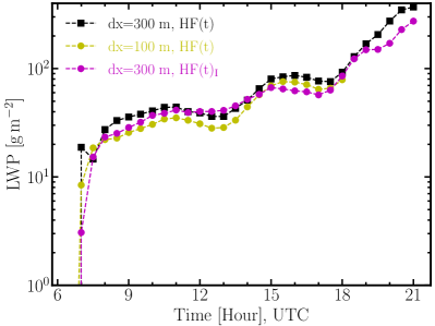
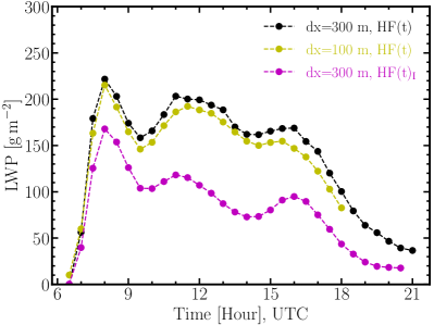
We also perform WRF-LES with interactive surface heat fluxes estimated from a prescribed constant SST from ERA5 and model simulated atmospheric states for both cases. A constant ERA5-SST is used here because ERA5-SST does not vary at the location of dropsonde center from 06:00 UTC to 21:00 UTC. Figure 16(a) shows that surface heat fluxes ($\rm{SHF_{\rm I}}$ and $\rm{LHF_{\rm I}}$) calculated within the WRF-LES surface scheme (Beljaars 1995; Chen and Dudhia 2001) are close to the ones from ERA5, leading to a similar LWP (Figure 24) and meteorological states (Figure 25) for the February 28 case. The frequency of LWP from simulation 0228E (prescribed $\rm{HF}(t)$ from ERA5) and 0228F ($\rm{HF}(t)$ calculated interactively within WRF-LES) agree excellently with the RSP measurement as shown in Figure 12(a). For the March 1 case, the surface latent heat flux from WRF-LES is substantially weaker than the one from ERA5 (Figure 16(b)), resulting in a drier BL (Figure 25) and smaller LWP (Figure 24). The frequency of LWP from simulation 0301F agrees better with RSP than that from 0301E. Nevertheless, we use prescribed surface heat fluxes from ERA5 in our LES because there is no direct measurement of surface heat fluxes from the ACTIVATE campaign. We aim to unravel aerosol-meteorology-cloud interactions and to improve its parameterizations in the Earth System Models by using LES constrained by ACTIVATE measurements and reanalysis data.

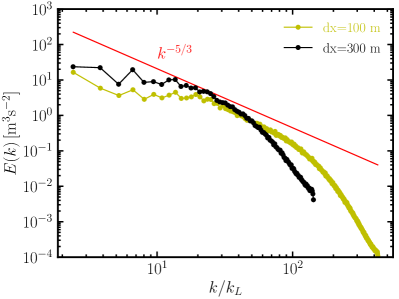
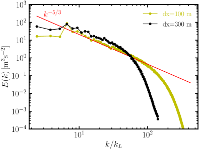
Simulations with finer horizontal resolution ($dx=100\,\rm{m}$) yields similar LWP (Figure 24) and almost identical vertical profiles (Figure 25) as the ones with $dx=300\,\rm{m}$ for both cases. The energy power spectra at 1 km height during the measurement time is shown in Figure 26. As expected, a larger inertial range is observed for simulation with $dx=100\,\rm{m}$. Nevertheless, this does not affect the simulated LWP and BL thermodynamics, which justifies our use of $dx=300\,\rm{m}$.

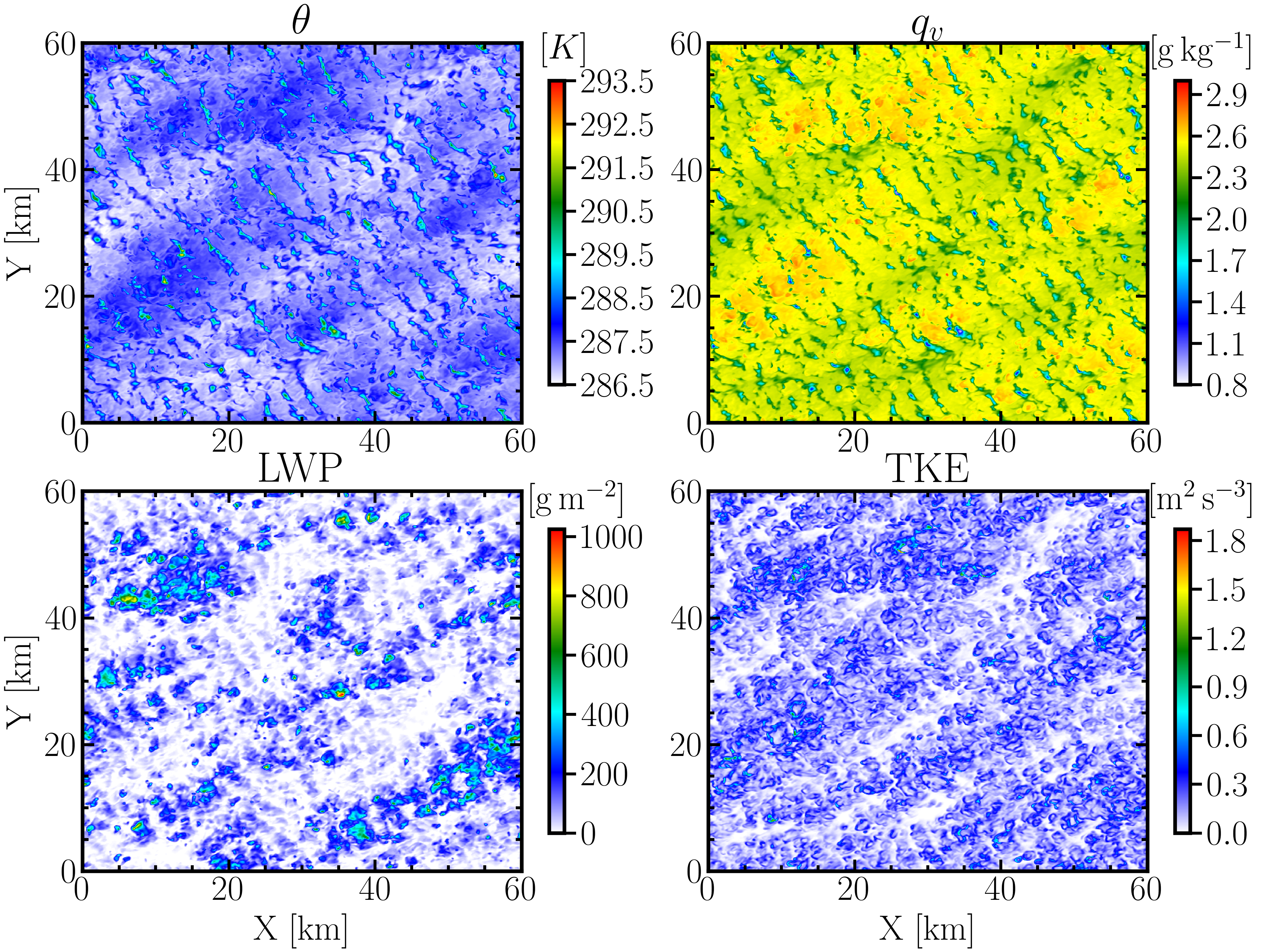
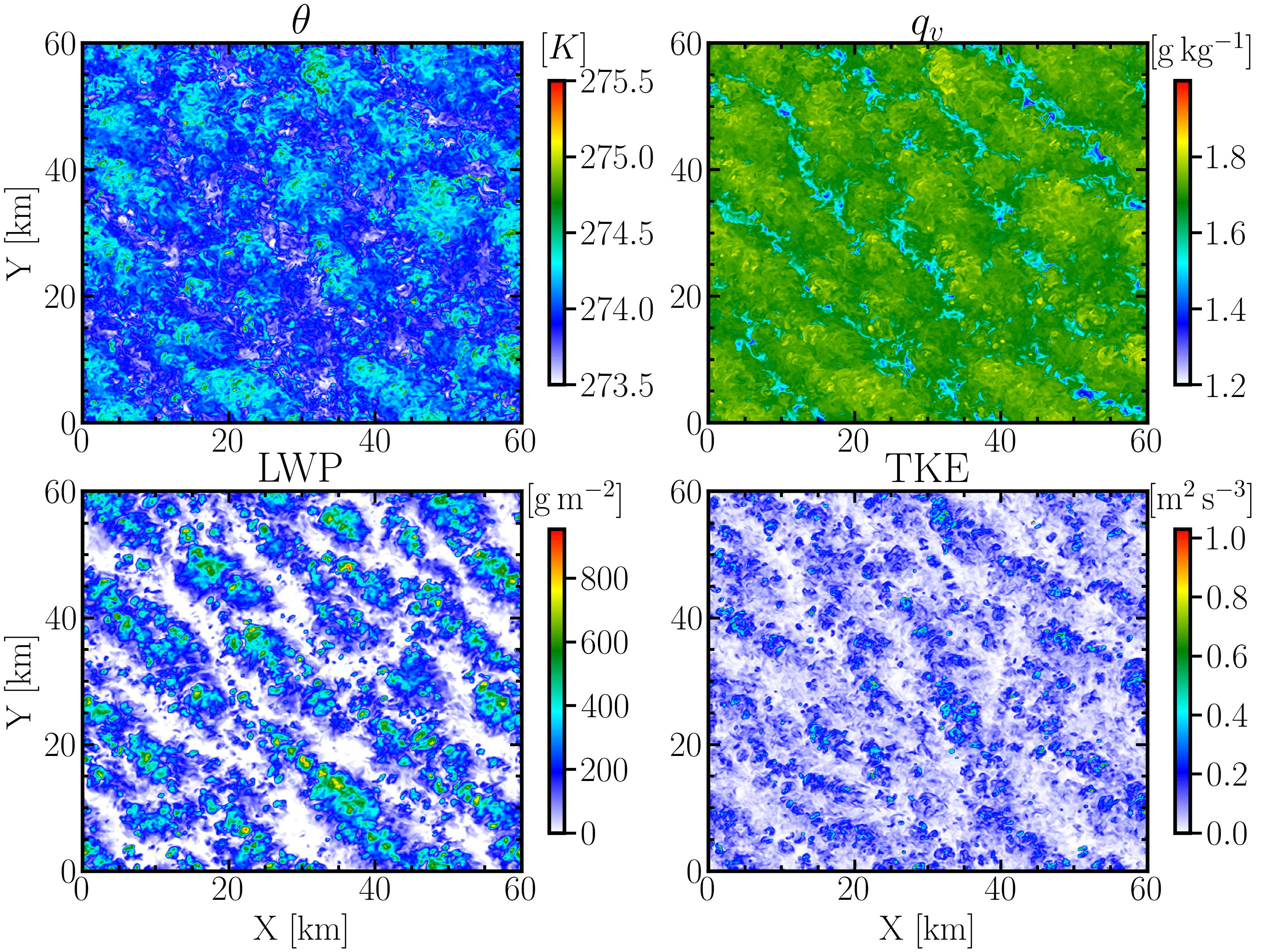
Figure 28 shows the instantaneous field of $\theta$, $q_{v}$, $q_{c}$, and TKE at UTC 16:00 and 2.5 km (near cloud top) for the February 28 case (simulation 0228G with dx=100 m). The thermodynamics fields exhibits same spatial patterns as TKE. Same for the March 1 case (simulation 0301G with dx=100 m) at 1.5 km as shown in Figure 29.

Figure 16: Surface heat fluxes from ERA5 (black lines) reanalysis data at the center of dropsonde circle on (a) February 28 and (b) March 1. Solid dots and squares represent heat fluxes at the center of dropsonde circles calculated based on the Z98 algorithm. Blue stars and pluses represent surface sensible $\rm{SHF(t)_{I}}$ and latent heat $\rm{LHF(t)_{I}}$ fluxes output from WRF-LES (0228F and 0301F), respectively.

Table 3: Surface heat fluxes during the dropsonde measurement time. “Flux” represents moisture and heat fluxes calculated from LES $\overline{w^{\prime}q_{v}^{\prime}}$ and $\overline{w^{\prime}\theta^{\prime}}$ (0228E and 0301E) at the bottom model layer, respectively.

Case	SHF [$\rm{W\,m}^{-2}$]				LHF [$\rm{W\,m}^{-2}$]
	ERA5	Z98	I	Flux	ERA5	Z98	I	Flux
0228	59.7	71.7	77.2	64.4	250.7	259.5	306.6	273.1
0301	234.1	243.4	220.3	232.2	402.3	409.2	318.4	406.7

5 Turbulent fluxes: validating LES against aircraft in-situ measurements

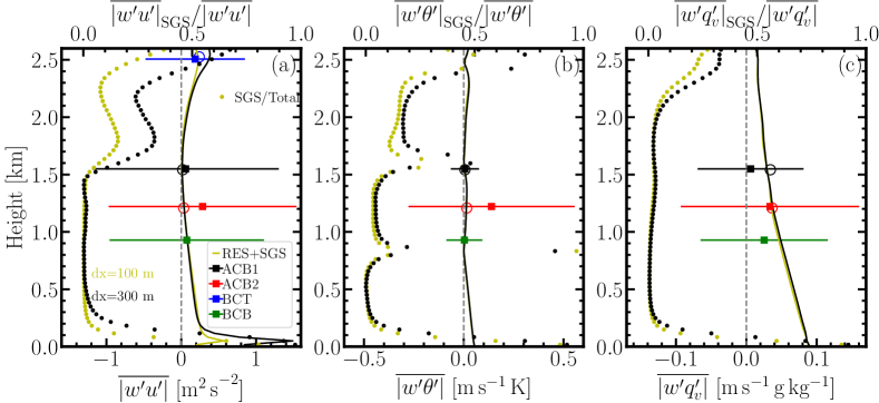
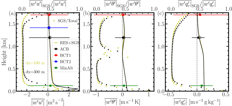
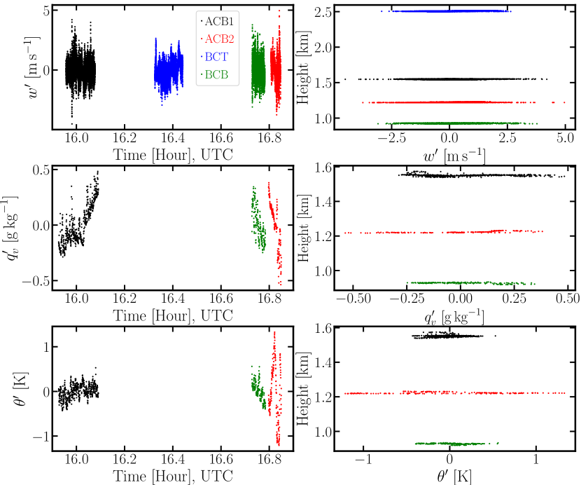
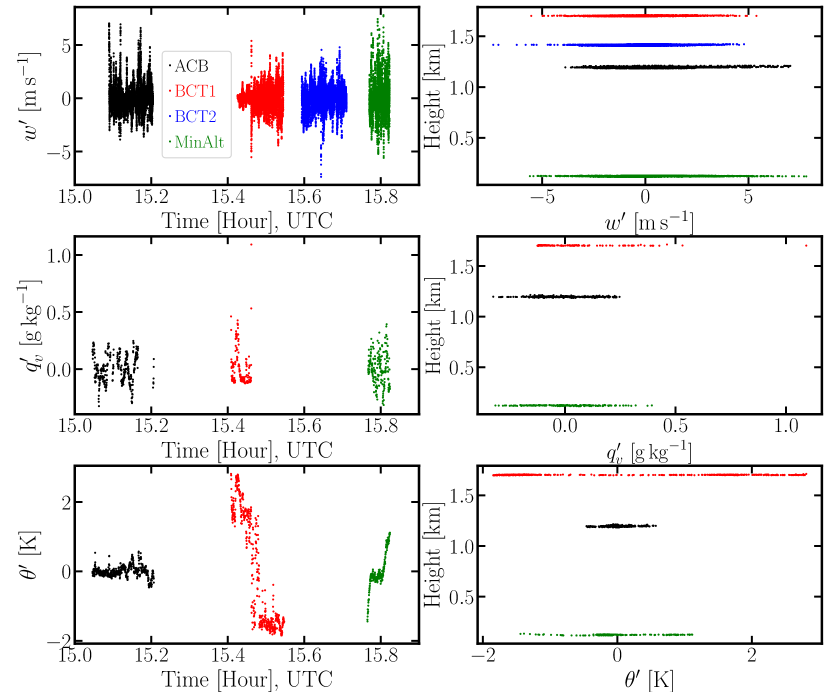
To validate LES against in-situ measurements during the ACTIVATE campaign, we compare the measured turbulent fluxes from the Falcon aircraft flying in the BL to the ones from LES. We select two above cloud-base (ACB), one below cloud-top (BCT), and one below cloud-base (BCB) flight legs during the dropsonde measurement time (16:00-17:00 UTC) on February 28. The time series and vertical profiles of $w^{\prime}$, $q_{v}^{\prime}$ and $\theta^{\prime}$ from the four flight legs (ACB1, ACB2, BCT, BCB) are shown in Figure 30. The sampling time and altitude variation of each flight leg is about 10 minutes or less and about 17 m (Table 4), respectively. Since the vertical layer thickness of LES is about 33 m within BL, we compare turbulent fluxes at the LES layer center that is closest to the height of each flight leg. The closest LES snapshot (every 30 minutes) to the flight sampling time is used for comparison. To calculate turbulent fluxes from measurements, the sampling time of $T$ and $q_{v}$ are mapped to that of averaged wind speed, which has 20 times higher sampling frequency. Figure 17 shows the comparison of turbulent fluxes between the Falcon measurements and LES. The sampling frequency of $T$ and $q_{v}$ is 1 Hz, which is equivalent to a spatial distance of $100\,\rm{m}$ given that the flight speed is about $100\,{\rm m\,s}^{-1}$. Such a spatial distance is comparable to the mesh size of LES. The LES is able to reproduce $\overline{w^{\prime}u^{\prime}}$ and $\overline{w^{\prime}\theta^{\prime}}$ measured during flight legs ACB1, BCT, and BCB. It captures the measured $\overline{w^{\prime}q_{v}^{\prime}}$ at flight leg ACB2. The measured $\overline{w^{\prime}u^{\prime}}$, $\overline{w^{\prime}\theta^{\prime}}$ and $\overline{w^{\prime}q_{v}^{\prime}}$ agree well with the ones from LES for the March 1 case, as shown in Figure 18.

Comparison of turbulent fluxes between simulation 0228E ($dx=300\,\rm{m}$) and 0228G ($dx=100\,\rm{m}$) is also shown in Figure 17. The parameterized subgrid-scale (SGS) turbulent fluxes are strong within the surface layer for both simulations, above which all the eddies are resolved by LES as suggested by the ratio between SGS and the total fluxes (i.e. yellow and black dots). $\overline{w^{\prime}u^{\prime}}$ within the surface layer is strongly mesh-size dependent, which is not the case for $\overline{w^{\prime}\theta^{\prime}}$ and $\overline{w^{\prime}q_{v}^{\prime}}$. Therefore, the simulation with dx=300 m yields the same LWP as the one with dx=100 m as discussed in section 4.4.3. The same conclusion can be drawn for the March 1 case as shown in Figure 18.

Figure 17: (a) momentum, (b) heat, and (c) moisture fluxes within BL during dropsonde measurement time for the February 28 case. Open circles represent total fluxes, i.e., resolved (RES) plus sub-grid scale (SGS) fluxes, from simulation 0228G. Solid squares represent the ones from different flight legs (“ACB”, “BCT” and “BCB” denotes above cloud-base, below cloud-top,and below cloud-base, respectively). The error bars represent one standard deviation of fluxes. Solid and dotted lines represent the total fluxes and the ratio between SGS and the total fluxes from LES, respectively. The closest snapshots in both time and height from simulation 0228G are used to compare to the measurements. $\overline{w^{\prime}\theta^{\prime}}$ and $\overline{w^{\prime}q_{v}^{\prime}}$ from Falcon measurements are calculated by matching the sampling time of $q_{v}$ and $\theta$ to the averaged $w$, respectively. The time series and vertical profiles of $w^{\prime}$, $q_{v}^{\prime}$ and $\theta^{\prime}$ from the measurements are shown in Figure 30. Flight time and height of the four flight legs are listed in Table 4. $\overline{w^{\prime}q_{v}^{\prime}}$ and $\overline{w^{\prime}\theta^{\prime}}$ from the BCT leg is not shown due to limited sampling. Vertical profiles from LES are averaged during the dropsonde measurement time. Moisture and heat fluxes calculated from the bottom layer of LES $\overline{w^{\prime}q_{v}^{\prime}}$ and $\overline{w^{\prime}\theta^{\prime}}$ (0228E and 0301E), respectively, are listed in Table 3.

Figure 18: Same as Figure 17 but for the March 1 case (simulation 0301G and 0301E). $\overline{w^{\prime}q_{v}^{\prime}}$ is not shown for the flight leg BCT2 because $q_{v}$ was not measured. “MinAlt” denotes minimum altitude ($\sim 150\,{\rm m}$). The corresponding time series and vertical profiles of the measured $w^{\prime}$, $\theta^{\prime}$, and $q_{v}^{\prime}$ are shown in Figure 31.

6 Discussion and conclusions

We have reported two contrasting cold air outbreak (CAO) cases observed during the ACTIVATE field campaign and the corresponding WRF-LES modeling of them. The February 28 case is characterized by weaker turbulent surface heat fluxes (${\rm SHF=79.91\,W\,m}^{-2}$ and ${\rm LHF=305.02\,W\,m}^{-2}$) than those of the March 1 case (${\rm SHF=231.76\,W\,m}^{-2}$ and ${\rm LHF=382.18\,W\,m}^{-2}$). The divergence is on the order of $10^{-5}\,{\rm s}^{-1}$ for both cases, which is about 10 times larger than common marine cases (e.g., $\bar{D}\approx 10^{-6}\,{\rm s}^{-1}$ in the DYCOMS-II case simulated by Wang and Feingold (2009)) and about two times larger than the CAO case in de Roode et al. (2019). A deeper, warmer, and more humid boundary layer was observed for the February 28 event than the one on March 1.

To examine and validate different prescribed forcing options to drive WRF-LES, we first evaluate divergence obtained from the ERA5 reanalysis data against the one derived from dropsonde measurements for the two CAO cases. The divergence profile and the corresponding vertical velocity obtained from ERA5 reanalysis data at the center of dropsonde circle are able to capture the structure of the ones estimated from dropsonde measurements for the March 1 case. This gives us the confidence to adopt the time-varying divergence profiles from ERA5 to drive our WRF-LES.

Since the surface turbulent heat fluxes are partly determined by SST, we compare SST from ERA5 to the one from satellite retrievals. They agree very well for both February 28 and March 1 cases. Therefore, SST from ERA5 together with the 10 m temperature, water vapor mixing ratio, and wind speed from dropsonde measurements are used to calculate heat fluxes for the March 1 case and those from ERA5 for the February 28 case using the bulk aerodynamic algorithms from Zeng et al. (1998). The estimated sensible and latent heat fluxes agree well with the ones directly obtained from ERA5 reanalysis data for the March 1 case case. They are underestimated by about $30\%$ compared to the ERA5 heat fluxes for the February 28 case.

By applying the surface heat fluxes, large-scale temperature and moisture advective tendencies, and wind relaxation adjustments from ERA5 to the WRF-LES, the simulated meteorological states for both CAO cases match the ERA5 reanalysis data and the ACTIVATE field campaign measurements. We also conduct WRF-LES sensitivity simulations on the surface fluxes and divergence and find that the divergence is important in suppressing the evolution of the boundary layer and achieves the observed states of the boundary layer for this case, while surface heat fluxes are more influential for the simulated LWP. The frequency of LWP produced from our WRF-LES agrees reasonably well with the measured ones from the ACTIVATE campaign for both the February 28 case. Since the large-scale tendencies profiles vary with time for the two CAO cases, it is important to apply time-varying tendencies to the WRF-LES instead of constant ones.

In summary, with initial conditions, large-scale forcings, and turbulent surface heat fluxes obtained from ERA5 and validated by ACTIVATE airborne measurements, WRF-LES is able to reproduce the observed boundary-layer meteorological states and LWP for two contrasting CAO cases. This manifests the meteorological impact on marine boundary layer and clouds associated with CAO over WNAO. This study (Part 1) paves the path to further investigation of aerosol effects on cloud microphysics during the CAO events to be reported in the forthcoming companion paper (Part 2).

Appendix A Dropsonde measurements

This appendix is to review the method being adopted to calculate divergence $D$ from the dropsonde measurements and to test statistical convergence of $D$ to the number of dropsondes used in the calculation.

The integral form of Equation (7) is

$$\int{\bm{\nabla}}\cdot{\bm{u}}{\rm d}S=0.$$ (14)

Thus,

$$\int\left(\frac{\partial u}{\partial x}+\frac{\partial v}{\partial y}\right){\rm d}S=-\int\frac{\partial w}{\partial z}{\rm d}S=-A\frac{\partial w}{\partial z}.$$ (15)

According to the Stokes theorem, Equation (15) can be written as

$$\frac{\partial w}{\partial z}=-D=-\frac{1}{A}\oint_{l}v_{n}{\rm d}l.$$ (16)

Based on Equation (16), Lenschow et al. (2007) noted that the most efficient flight track is a circle-like shape since the circle has the largest enclosed area of any closed curve and the turning rate of flight is slow. Such a method to calculate $D$ is called the “linear integral method”. This method requires a closed and circular flight track and a linearly evolving wind speed, none of which can be satisfied. Therefore, Lenschow et al. (2007) developed the “regression method”, which can alleviate the requirements of the linear integral method. The first order Taylor expansion of horizontal wind velocity ${\bm{v}}={\bm{v}}(u,v)$ at the dropsondes center is

$${\bm{v}}={\bm{v}_{0}}+\frac{\partial{\bm{v}}}{\partial x}\Delta x+\frac{\partial{\bm{v}}}{\partial y}\Delta y+\frac{\partial{\bm{v}}}{\partial t}\Delta t,$$ (17)

where $\Delta x$ and $\Delta y$ are the eastward and northwest displacements from the center of dropsondes. Assuming a stationary state, the term $\frac{\partial{\bm{v}}}{\partial t}\Delta t$ can be neglected. This assumption suggests that all the dropsondes should be released simultaneously, which is not feasible experimentally. The sampling lag in space and time between different dropsondes may cause error of calculating $\bar{D}$. However, Bony and Stevens (2019) demonstrated that the stationarity assumption is not bad.

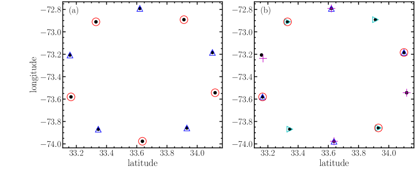
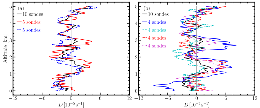
We then test the sensitivity of $\bar{D}$ to the number of dropsondes used in the calculation. Figure 19 shows the circular distribution of 10 dropsondes (black solid dots) for the February 28 case. Here, only 10 dropsondes are used to calculate the divergence because two (out of the 11 dropsondes) were released at the same location. We select two subsets as shown in Figure 19(a). The corresponding $\bar{D}$ is shown in Figure 20(a). $\bar{D}$ derived from the 5-dropsonde circle agrees with that from the 10-dropsonde circle. We also test four subsets of 4-dropsonde circles, as shown in Figure 19(b), and the corresponding $\bar{D}$ is shown in Figure 20(b). Same as the 5-dropsonde circles, 4-dropsonde subset agree with the 10-dropsonde circle even though the individual subsets exhibit differences.

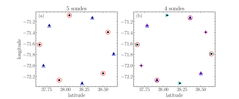
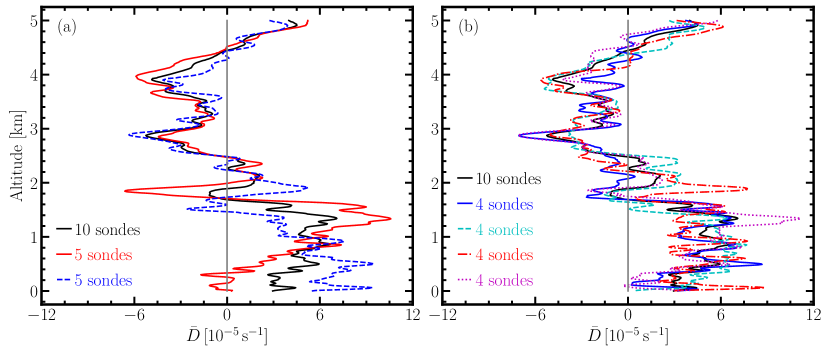
We also apply the same analysis to dropsonde measurements being carried out on the March 1 case as shown in Figure 21 and Figure 22. $\bar{D}$ derived from the 5-dropsonde circle agrees with that from the 10-dropsonde circle above the inversion layer but differs within the boundary layer. The difference is even larger between the two different sets of 5-dropsonde circles (red and blue curves in Figure 22(a)) in the boundary layer. Interestingly, $\bar{D}$ from the 4-dropsonde subset (Figure 22(b)) is closer to the one derived from the 10-dropsonde. Therefore, reducing the total number of dropsondes in a circle results in statistical uncertainties. Bony and Stevens (2019) suggested that at least 12 dropsondes are needed to estimate $\bar{D}$. More dropsondes can indeed improve the accuracy of the estimation in the tropics as shown in Figure 5 of Bony and Stevens (2019). However, the additional two dropsondes are not expected to make a big difference.

Figure 19: Latitude and longitude coordinates of dropsondes released on February 28 case. Black dots represent the 10 dropsondes. (a): Red circles and blue triangles represent two subsets of 5 dropsondes, respectively. (b): Red circles, blue triangles, cyan triangles, and red crosses represent four subsets of 4 dropsondes, respectively.

Figure 20: Corresponding $\bar{D}$ profiles derived from dropsonde measurements shown in Figure 19.

Figure 21: Same as Figure 19 but for the March 1 case.

Figure 22: Corresponding $\bar{D}$ profiles derived from groups of dropsondes shown in Figure 21.

Appendix B Surface heat fluxes: ERA5 versus MERRA-2

Figure 23 shows the comparison of heat fluxes between ERA5 and MERRA-2 reanalysis data. MERRA-2 underestimates the heat fluxes compared to ERA5.

Figure 23: Comparison of heat fluxes between ERA5 and MERRA-2 reanalysis data at 15:00 UTC for the February 28 case (black squares) anad 16:00 UTC for the March 1 case (red squares). Heat fluxes from the MERRA-2 reanalysis data are averaged between 16:30 and 17:30 for the February 28 case and between 14:30 and 15:30 for the March 1 case.

Appendix C Horizontal resolution and interactive surface heat fluxes

Figure 24 and Figure 25 shows the horizontal resolution and interactive surface heat fluxes dependency for both cases. The interactive heat fluxes result in smaller LWP and IWP. This is due to smaller heat fluxes shown in Figure 16.

Figure 24: Horizontal resolution and interactive surface heat fluxes dependency for the February 28 (left-hand side) and March 01 cases (right-hand side). $\rm{SHF}(t)$ and $\rm{LHF}(t)$ from ERA5 are adopted. $\rm{HF(t)_{I}}$ denotes the heat fluxes calculated interactively with ERA5-SST as input. Black, yellow, and magenta lines represent simulation 0228E (0301E), 0228G (0301G), and 0228F (0301F), respectively.

Figure 25: Vertical profiles for the February 28 (upper row) and March 1 (lower row) case during the dropsonde measurement. Same simulations as in Figure 24.

Figure 26: Energy power spectra at $H=1{\rm km}$ averaged during the measurement time for the February 28 (left-hand side, 16:00-17:00 UTC) and March 1 (right-hand side, 15:00-16:00 UTC) case. The abscissa is normalized by $k_{L}=2\pi/L_{x}$ to demonstrate at which length scale the eddies are not resolved, i.e., $E(k)$ deviates away from the Kolmogorov scaling $k^{-5/3}$ (red curve). Black and red yellow lines represent simulation 0228E (0301E) and 0228G (0301G), respectively.

Appendix D Vertical profiles for LES with different forcing

Figure 27 shows the evolution of vertical profiles of the meteorological state for simulations shown in Figure 10.

Figure 27: Evolution of domain-averaged vertical profiles from the WRF-LES simulation with the corresponding input forcings shown in Figure 9 for the February 28 case. The rainbow color scheme represents the time evolution (06:00-21:00 UTC): from purple to red. The solid black line represents the ERA5 reanalysis data and the dashed one represent the WRF-LES averaged during the measurement time. The grey curve represents the dropsonde measurement. From the top to the bottom, rows represent the simulation with no forcing, only advective tendencies ($\partial\bar{\theta}/\partial t$ and $\partial\bar{q}_{v}/\partial t$), only relaxation of $u$ and $v$, and advective tendencies ($\partial\bar{\theta}/\partial t$ $\partial\bar{q}_{v}/\partial t$) plus $\bar{u}$ and $\bar{v}$ relaxation to $u_{\rm ERA5}$ and $v_{\rm ERA5}$, respectively.

Figure 28 shows horizontal cross-section of $\theta$, $q_{v}$, $q_{c}$, and TKE at UTC 16:00 and a height of 2.5 km for the February 28 case (simulation 0228G). Those for the March 1 case (simulation 0301G) are shown in Figure 29.

Appendix E Instantaneous fields and in-situ measurements

Figure 28 and Figure 29 show instantaneous fields for the February 28 and March 1 cases, respectively. Time series and vertical profiles of $w^{\prime}$, $q_{v}^{\prime}$, and $\theta^{\prime}$ from the Falcon measurements are shown in Figure 30 and Figure 31 for the two cases.

Figure 28: Horizontal cross-section of $\theta$, $q_{v}$, $q_{c}$, and TKE at UTC 16:00 and 2.5 km (near cloud top) for the February 28 case (simulation 0228G).

Figure 29: Same as Figure 28 but for the March 1 case (simulation 0301G) at 1.5 km.

Table 4: Falcon flight legs for the February 28 and March 1 cases. “ACB”, “BCT”, “BCB”, “MinAlt” denotes above cloud-base, below cloud-top, below cloud-base, and minimum altitude, respectively.

Case	Flight legs	Time [s], UTC	Height [m]
	ABC1	15:55:35-16:05:28	1538.37-1555.35
0228	ABC2	16:47:51-16:51:00	1217.93-1230.76
	BCT	16:18:41-16:26:56	2496.92-2514.76
	BCB	16:43:41-16:47:03	918.58-934.12
	ABC	15:02:47-15:12:24	1185.53-1210.00
0301	BCT1	15:24:31-15:32:51	1697.50-1708.11
	BCT2	15:34:07-15:42:44	1405.56-1423.46
	MinAlt	15:45:54-15:49:26	116.56-128.13

Figure 30: Time series and vertical profiles of $w^{\prime}$, $q_{v}^{\prime}$, and $\theta^{\prime}$ from the Falcon measurements for the February 28 case. Flight time and height of each leg are listed in Table 4.

Figure 31: Same as Figure 30 but for the March 1 case. Flight time and height of each leg are listed in Table 4.

References

- Ackerman et al. (2009) Ackerman, A. S., and Coauthors, 2009: Large-eddy simulations of a drizzling, stratocumulus-topped marine boundary layer. Monthly Weather Review, 137 (3), 1083–1110.
- Agee (1987) Agee, E. M., 1987: Mesoscale cellular convection over the oceans. Dynamics of atmospheres and oceans, 10 (4), 317–341.
- Alexandrov et al. (2012) Alexandrov, M. D., B. Cairns, C. Emde, A. S. Ackerman, and B. van Diedenhoven, 2012: Accuracy assessments of cloud droplet size retrievals from polarized reflectance measurements by the research scanning polarimeter. Remote sensing of environment, 125, 92–111.
- Alexandrov et al. (2018) Alexandrov, M. D., and Coauthors, 2018: Retrievals of cloud droplet size from the research scanning polarimeter data: Validation using in situ measurements. Remote Sensing of Environment, 210, 76–95.
- Augstein et al. (1973) Augstein, E., H. Riehl, F. Ostapoff, and V. Wagner, 1973: Mass and energy transports in an undisturbed atlantic trade-wind flow. Monthly Weather Review, 101 (2), 101–111.
- Beljaars (1995) Beljaars, A. C., 1995: The parametrization of surface fluxes in large-scale models under free convection. Quarterly Journal of the Royal Meteorological Society, 121 (522), 255–270.
- Bony and Stevens (2019) Bony, S., and B. Stevens, 2019: Measuring area-averaged vertical motions with dropsondes. Journal of the Atmospheric Sciences, 76 (3), 767–783.
- Bony et al. (2017) Bony, S., B. Stevens, and D. Carlson, 2017: WMO Bulletin, 66, 8–11.
- Boucher et al. (2013) Boucher, O., and Coauthors, 2013: Clouds and aerosols. Climate change 2013: the physical science basis. Contribution of Working Group I to the Fifth Assessment Report of the Intergovernmental Panel on Climate Change, Cambridge University Press, 571–657.
- Bretherton and Blossey (2017) Bretherton, C., and P. Blossey, 2017: Understanding mesoscale aggregation of shallow cumulus convection using large-eddy simulation. Journal of Advances in Modeling Earth Systems, 9 (8), 2798–2821.
- Bretherton et al. (1999) Bretherton, C. S., S. K. Krueger, M. C. Wyant, P. Bechtold, E. Van Meijgaard, B. Stevens, and J. Teixeira, 1999: A gcss boundary-layer cloud model intercomparison study of the first astex lagrangian experiment. Boundary-Layer Meteorology, 93 (3), 341–380.
- Brilouet et al. (2020) Brilouet, P.-E., P. Durand, G. Canut, and N. Fourrié, 2020: Organized turbulence in a cold-air outbreak: Evaluating a large-eddy simulation with respect to airborne measurements. Boundary-Layer Meteorology, 1–35.
- Brown et al. (2002) Brown, A., and Coauthors, 2002: Large-eddy simulation of the diurnal cycle of shallow cumulus convection over land. Quarterly Journal of the Royal Meteorological Society: A journal of the atmospheric sciences, applied meteorology and physical oceanography, 128 (582), 1075–1093.
- Chellappan et al. (2021) Chellappan, S., and Coauthors, 2021: On assessing era5 and merra2 representations of cold-air outbreaks across the gulf stream. Geophysical Research Letters.
- Chen and Dudhia (2001) Chen, F., and J. Dudhia, 2001: Coupling an advanced land surface–hydrology model with the penn state–ncar mm5 modeling system. part i: Model implementation and sensitivity. Monthly weather review, 129 (4), 569–585.
- Corral et al. (2021) Corral, A. F., and Coauthors, 2021: An overview of atmospheric features over the western north atlantic ocean and north american east coast–part 1: Analysis of aerosols, gases, and wet deposition chemistry. Journal of Geophysical Research: Atmospheres, e2020JD032592.
- de Roode et al. (2019) de Roode, S. R., and Coauthors, 2019: Turbulent transport in the gray zone: A large eddy model intercomparison study of the constrain cold air outbreak case. Journal of Advances in Modeling Earth Systems, 11 (3), 597–623.
- Endo et al. (2015) Endo, S., and Coauthors, 2015: RACORO continental boundary layer cloud investigations: 2. large-eddy simulations of cumulus clouds and evaluation with in situ and ground-based observations. Journal of Geophysical Research: Atmospheres, 120 (12), 5993–6014.
- Gelaro et al. (2017) Gelaro, R., and Coauthors, 2017: The modern-era retrospective analysis for research and applications, version 2 (merra-2). Journal of climate, 30 (14), 5419–5454.
- Global Modeling and Assimilation Office (2015) (GMAO) Global Modeling and Assimilation Office (GMAO), 2015: Merra-2 inst33dasmnv: 3d, 3-hourly, instantaneous, model-level, assimilation, assimilated meteorological fields v5.12.4. Greenbelt, MD, USA, Goddard Earth Sciences Data and Information Services Center (GES DISC), URL https://disc.gsfc.nasa.gov/datasets/M2I3NVASM˙5.12.4/summary, accessed March 10, 2021, 10.5067/WWQSXQ8IVFW8.
- Gryschka et al. (2014) Gryschka, M., J. Fricke, and S. Raasch, 2014: On the impact of forced roll convection on vertical turbulent transport in cold air outbreaks. Journal of Geophysical Research: Atmospheres, 119 (22), 12–513.
- Gryschka and Raasch (2005) Gryschka, M., and S. Raasch, 2005: Roll convection during a cold air outbreak: A large eddy simulation with stationary model domain. Geophysical research letters, 32 (14).
- Heinze et al. (2017) Heinze, R., C. Moseley, L. N. Böske, S. K. Muppa, V. Maurer, S. Raasch, and B. Stevens, 2017: Evaluation of large-eddy simulations forced with mesoscale model output for a multi-week period during a measurement campaign. Atmospheric Chemistry and Physics, 17 (11), 7083–7109.
- Hersbach et al. (2020) Hersbach, H., and Coauthors, 2020: The era5 global reanalysis. Quarterly Journal of the Royal Meteorological Society, 146 (730), 1999–2049, https://doi.org/10.1002/qj.3803, URL https://rmets.onlinelibrary.wiley.com/doi/abs/10.1002/qj.3803.
- Hirahara et al. (2016) Hirahara, S., M. A. Balmaseda, E. de Boisseson, and H. Hersbach, 2016: 26 sea surface temperature and sea ice concentration for era5.
- Holland and Rasmusson (1973) Holland, J. Z., and E. M. Rasmusson, 1973: Measurements of the atmospheric mass, energy, and momentum budgets over a 500-kilometer square of tropical ocean. Monthly Weather Review, 101 (1), 44–55.
- Holthuijsen et al. (2012) Holthuijsen, L. H., M. D. Powell, and J. D. Pietrzak, 2012: Wind and waves in extreme hurricanes. Journal of Geophysical Research: Oceans, 117 (C9).
- Knop et al. (2021) Knop, I., S. E. Bansmer, V. Hahn, and C. Voigt, 2021: Comparison of different droplet measurement techniques in the braunschweig icing wind tunnel. Atmospheric Measurement Techniques, 14 (2), 1761–1781.
- Lenschow et al. (1999) Lenschow, D. H., P. B. Krummel, and S. T. Siems, 1999: Measuring entrainment, divergence, and vorticity on the mesoscale from aircraft. Journal of atmospheric and oceanic technology, 16 (10), 1384–1400.
- Lenschow et al. (2007) Lenschow, D. H., V. Savic-Jovcic, and B. Stevens, 2007: Divergence and vorticity from aircraft air motion measurements. Journal of atmospheric and oceanic technology, 24 (12), 2062–2072.
- Li et al. (2018) Li, X.-Y., A. Brandenburg, G. Svensson, N. E. Haugen, B. Mehlig, and I. Rogachevskii, 2018: Effect of turbulence on collisional growth of cloud droplets. Journal of the Atmospheric Sciences, 75 (10), 3469–3487.
- Li et al. (2020) Li, X.-Y., A. Brandenburg, G. Svensson, N. E. Haugen, B. Mehlig, and I. Rogachevskii, 2020: Condensational and collisional growth of cloud droplets in a turbulent environment. Journal of the Atmospheric Sciences, 77 (1), 337–353.
- Li et al. (2019) Li, X.-Y., G. Svensson, A. Brandenburg, and N. E. Haugen, 2019: Cloud-droplet growth due to supersaturation fluctuations in stratiform clouds. Atmospheric Chemistry and Physics, 19 (1), 639–648.
- Liu et al. (2004) Liu, A., G. Moore, K. Tsuboki, and I. Renfrew, 2004: A high-resolution simulation of convective roll clouds during a cold-air outbreak. Geophysical Research Letters, 31 (3).
- Morrison et al. (2009) Morrison, H., G. Thompson, and V. Tatarskii, 2009: Impact of cloud microphysics on the development of trailing stratiform precipitation in a simulated squall line: Comparison of one-and two-moment schemes. Monthly weather review, 137 (3), 991–1007.
- National Center for Atmospheric Research (2021) National Center for Atmospheric Research, 2021: Avaps dropsondes. URL https://www.eol.ucar.edu/content/avaps-dropsondes, accessed March 16, 2021.
- National Centers for Environmental Information (2008) National Centers for Environmental Information, 2008: Remote sensing systems (remss). ghrsst level 4 mwiroi global foundation sea surface temperature and analysis version 5.0 from remss (gds versions 1 and 2). URL https://www.ncei.noaa.gov/archive/accession/GHRSST-MW˙IR˙OI-REMSS-L4-GLOB, accessed March 16, 2021.
- Neggers et al. (2012) Neggers, R. A., A. Siebesma, and T. Heus, 2012: Continuous single-column model evaluation at a permanent meteorological supersite. Bulletin of the American Meteorological Society, 93 (9), 1389–1400.
- Painemal et al. (2021) Painemal, D., and Coauthors, 2021: An overview of atmospheric features over the western north atlantic ocean and north american east coast–part 2: Circulation, boundary layer, and clouds. Journal of Geophysical Research: Atmospheres, e2020JD033423.
- Papritz et al. (2015) Papritz, L., S. Pfahl, H. Sodemann, and H. Wernli, 2015: A climatology of cold air outbreaks and their impact on air–sea heat fluxes in the high-latitude south pacific. Journal of Climate, 28 (1), 342–364.
- Powell et al. (2003) Powell, M. D., P. J. Vickery, and T. A. Reinhold, 2003: Reduced drag coefficient for high wind speeds in tropical cyclones. Nature, 422 (6929), 279–283.
- Quinn et al. (2021) Quinn, P. K., and Coauthors, 2021: Measurements from the rv ronald h. brown and related platforms as part of the atlantic tradewind ocean-atmosphere mesoscale interaction campaign (atomic). Earth System Science Data, 13 (4), 1759–1790.
- Rahn and Garreaud (2010) Rahn, D. A., and R. Garreaud, 2010: Marine boundary layer over the subtropical southeast pacific during vocals-rex–part 1: Mean structure and diurnal cycle. Atmospheric Chemistry and Physics, 10 (10), 4491–4506.
- Ramanathan et al. (1989) Ramanathan, V., R. D. Cess, E. F. Harrison, P. Minnis, B. R. Barkstrom, E. Ahmad, and D. Hartmann, 1989: Science, 243 (4887), 57–63.
- Randall and Cripe (1999) Randall, D. A., and D. G. Cripe, 1999: Alternative methods for specification of observed forcing in single-column models and cloud system models. Journal of Geophysical Research: Atmospheres, 104 (D20), 24 527–24 545.
- Richter et al. (2016) Richter, D. H., R. Bohac, and D. P. Stern, 2016: An assessment of the flux profile method for determining air–sea momentum and enthalpy fluxes from dropsonde data in tropical cyclones. Journal of the Atmospheric Sciences, 73 (7), 2665–2682.
- Schneider et al. (2017) Schneider, T., J. Teixeira, C. S. Bretherton, F. Brient, K. G. Pressel, C. Schär, and A. Siebesma, 2017: Nature Climate Change, 7 (1), 3–5.
- Seifert et al. (2015) Seifert, A., T. Heus, R. Pincus, and B. Stevens, 2015: Large-eddy simulation of the transient and near-equilibrium behavior of precipitating shallow convection. Journal of Advances in Modeling Earth Systems, 7 (4), 1918–1937.
- Shaw (2003) Shaw, R. A., 2003: Particle-turbulence interactions in atmospheric clouds. Annu. Rev. Fluid Mech., 35 (1), 183–227.
- Siebesma and Cuijpers (1995) Siebesma, A., and J. Cuijpers, 1995: Evaluation of parametric assumptions for shallow cumulus convection. Journal of Atmospheric Sciences, 52 (6), 650–666.
- Skamarock et al. (2019) Skamarock, W. C., and Coauthors, 2019: A description of the advanced research wrf model version 4. National Center for Atmospheric Research: Boulder, CO, USA, 145.
- Smith (1988) Smith, S. D., 1988: Coefficients for sea surface wind stress, heat flux, and wind profiles as a function of wind speed and temperature. Journal of Geophysical Research: Oceans, 93 (C12), 15 467–15 472.
- Sorooshian et al. (2019) Sorooshian, A., and Coauthors, 2019: Aerosol–cloud–meteorology interaction airborne field investigations: Using lessons learned from the us west coast in the design of activate off the us east coast. Bulletin of the American Meteorological Society, 100 (8), 1511–1528.
- Sorooshian et al. (2020) Sorooshian, A., and Coauthors, 2020: Atmospheric research over the western north atlantic ocean region and north american east coast: a review of past work and challenges ahead. Journal of Geophysical Research: Atmospheres, 125 (6), e2019JD031 626.
- Stevens and Bony (2013) Stevens, B., and S. Bony, 2013: Science, 340 (6136), 1053–1054.
- Stevens et al. (2019) Stevens, B., and Coauthors, 2019: A high-altitude long-range aircraft configured as a cloud observatory: The narval expeditions. Bulletin of the American Meteorological Society, 100 (6), 1061–1077.
- Stevens et al. (2002) Stevens, D. E., A. S. Ackerman, and C. S. Bretherton, 2002: Effects of domain size and numerical resolution on the simulation of shallow cumulus convection. Journal of the atmospheric sciences, 59 (23), 3285–3301.
- Taylor et al. (2019) Taylor, J. W., and Coauthors, 2019: Aerosol influences on low-level clouds in the west african monsoon. Atmospheric Chemistry and Physics, 19 (13), 8503–8522.
- Tomassini et al. (2017) Tomassini, L., P. R. Field, R. Honnert, S. Malardel, R. McTaggart-Cowan, K. Saitou, A. T. Noda, and A. Seifert, 2017: The “grey zone” cold air outbreak global model intercomparison: A cross evaluation using large-eddy simulations. Journal of Advances in Modeling Earth Systems, 9 (1), 39–64.
- Tornow et al. (2021) Tornow, F., A. S. Ackerman, and A. M. Fridlind, 2021: Preconditioning of overcast-to-broken cloud transitions by riming in marine cold air outbreaks. Atmospheric Chemistry and Physics, 21 (15), 12 049–12 067, 10.5194/acp-21-12049-2021.
- Van der Dussen et al. (2013) Van der Dussen, J., and Coauthors, 2013: The gass/euclipse model intercomparison of the stratocumulus transition as observed during astex: Les results. Journal of Advances in Modeling Earth Systems, 5 (3), 483–499.
- van Laar et al. (2019) van Laar, T. W., V. Schemann, and R. A. Neggers, 2019: Investigating the diurnal evolution of the cloud size distribution of continental cumulus convection using multiday les. Journal of the Atmospheric Sciences, 76 (3), 729–747.
- Wang and Feingold (2009) Wang, H., and G. Feingold, 2009: Modeling mesoscale cellular structures and drizzle in marine stratocumulus. part i: Impact of drizzle on the formation and evolution of open cells. Journal of the Atmospheric Sciences, 66 (11), 3237–3256.
- Wang et al. (2010) Wang, H., G. Feingold, R. Wood, and J. Kazil, 2010: Modelling microphysical and meteorological controls on precipitation and cloud cellular structures in southeast pacific stratocumulus. Atmospheric Chemistry and Physics, 10 (13), 6347–6362.
- Wang and McFarquhar (2008) Wang, H., and G. M. McFarquhar, 2008: Modeling aerosol effects on shallow cumulus convection under various meteorological conditions observed over the indian ocean and implications for development of mass-flux parameterizations for climate models. Journal of Geophysical Research: Atmospheres, 113 (D20).
- Wang et al. (2009) Wang, H., W. C. Skamarock, and G. Feingold, 2009: Evaluation of scalar advection schemes in the advanced research wrf model using large-eddy simulations of aerosol–cloud interactions. Monthly Weather Review, 137 (8), 2547–2558.
- Zeng et al. (1998) Zeng, X., M. Zhao, and R. E. Dickinson, 1998: Intercomparison of bulk aerodynamic algorithms for the computation of sea surface fluxes using toga coare and tao data. Journal of Climate, 11 (10), 2628–2644.