Dark Energy Survey Year 3 Results: Galaxy Sample for BAO Measurement

Abstract

In this paper we present and validate the galaxy sample used for the analysis of the Baryon Acoustic Oscillation signal (BAO) in the Dark Energy Survey (DES) Y3 data. The definition is based on a colour and redshift-dependent magnitude cut optimized to select galaxies at redshifts higher than 0.5, while ensuring a high quality determination. The sample covers ${\sim}\,4100$ square degrees to a depth of $i=22.3\ (AB)$ at $10\sigma$. It contains 7,031,993 galaxies in the redshift range from $z$= 0.6 to 1.1, with a mean effective redshift of 0.835. Redshifts are estimated with the machine learning algorithm DNF, and are validated using the VIPERS PDR2 sample. We find a mean redshift bias of $z_{\mathrm{bias}}{\sim}\,0.01$ and a mean uncertainty, in units of $1+z$, of $\sigma_{68}{\sim}\,0.03$. We evaluate the galaxy population of the sample, showing it is mostly built upon Elliptical to Sbc types. Furthermore, we find a low level of stellar contamination of $\lesssim 4\%$. We present the method used to mitigate the effect of spurious clustering coming from observing conditions and other large-scale systematics. We apply it to the BAO sample and calculate weights that are used to get a robust estimate of the galaxy clustering signal. This paper is one of a series dedicated to the analysis of the BAO signal in DES Y3. In the companion papers we present the galaxy mock catalogues used to calibrate the analysis and the angular diameter distance constraints obtained through the fitting to the BAO scale.

1 Introduction

Baryon Acoustic Oscillations (BAO) is one of the most remarkable predictions of the formation of structures in the Universe (Peebles & Yu, 1970; Sunyaev & Zeldovich, 1970; Bond & Efstathiou, 1984, 1987). Since its confirmation in the distribution of galaxies in 2005 (Eisenstein et al., 2005), BAO measurement has been one of the main scientific drivers in the design and construction of galaxy surveys.

BAO has already been detected several times in spectroscopic (Cole et al., 2005; Percival et al., 2007; Gaztañaga et al., 2009; Percival et al., 2010; Beutler et al., 2011; Blake et al., 2011; Ross et al., 2015; Alam et al., 2017) and photometric (Padmanabhan et al., 2007; Estrada et al., 2009; Hütsi, 2010; Crocce et al., 2011; Carnero et al., 2012; Abbott et al., 2019) data-sets, for galaxies, but also in the distribution of QSOs (Ata et al., 2018) and Lyman-alpha absorbers (Bautista et al., 2017), in a wide variety of redshifts, from $z=0.2$ to $z<3$. Estimates of the evolution of the BAO scale with time is a direct measurement of the expansion of the Universe and therefore, an excellent cosmology observable. All these measurements are compatible with the $\Lambda$CDM cosmological model and the existence of Dark Energy.

In this context, the Dark Energy Survey (DES: Flaugher 2005; DES Collaboration 2016) set as one of its main objectives to measure the BAO scale in the distribution of galaxies. In a previous release, in DES Year 1 (Abbott et al., 2019) we measured the BAO scale at an effective redshift of 0.81. This sample covered approx. 1400 square degrees; given the limited area, this detection had a low significance. In DES Year 3 (Y3), the data-set analysed here, the nominal footprint of approx. 5000 square degrees for the complete survey is covered, and we expect to reach a sensitivity to BAO of the same order as concurrent spectroscopic and photometric surveys. Furthermore, this measurement will be combined with the other DES cosmological observables to estimate the most precise measurements on Dark Energy by combination of BAO with Weak Lensing, Supernova Ia and Galaxy Clusters number counts.

One of the main difficulties in detecting BAO in photometric surveys is the smearing in the signal produced by the poor redshift determination. In this context, it is necessary to select a galaxy population that presents a prominent spectral feature that can be captured with broadband filters. Generally, the best practice is to select old, well-evolved galaxies with a significant Balmer break (Eisenstein et al., 2001; Vakili et al., 2019; Crocce et al., 2019; Zhou et al., 2020). This feature makes galaxies look very red, and they usually drive the target selection in galaxy surveys.

In Crocce et al. (2019), we developed a colour selection to select galaxies in the DES Y1 sample, calibrated through a set of synthetic SED distributions, optimized for redshifts $z>0.5$. In this new release, we apply the same colour selection, but put the focus in the improvement of ameliorating spurious clustering due to observing conditions. Since the sample now covers more than 4000 square degrees, with observations taken during three different years, variations on conditions like seeing, airmass, sky brightness, stellar density, or galactic extinction are expected to leave significant imprints in the galaxy clustering and therefore, robust corrections are needed. In DES Y3 we compute weights to correct for these effects, following the procedure developed in Elvin-Poole et al. (2018) for the DES Y1 lens sample, but to the DES Y3 BAO sample. Similar methods have also been applied to BOSS (Ross et al., 2011; Ross et al., 2017), eBOSS (Ross et al., 2020; Laurent et al., 2017) and DESI (Kitanidis et al., 2020) targets.

The structure of the paper is as follows: In Section 2 we present the parent DES Y3 data and next, in Section 3 we describe the BAO sample selection. In Section 4 we present the selection of the footprint. In Section 5 we present the photometric redshift (photo-$z$) definition and validation. In Section 6 we validate the sample. In Section 7 we summarize the blinding procedure, which is largely shared with other DES analyses. In Section 8 we present the analysis of mitigation of observational systematic effects and in Section 9 we show the 2-pt clustering signal in real space after the unblinding of the sample. Finally, we show our conclusions in Section 10. The BAO sample will be eventually released at https://des.ncsa.illinois.edu/releases together with all the DES Y3 products.

This paper accompanies a series of papers focused on the analysis of BAO distance in DES Y3 analysis. In Ferrero et al. (2021) we construct precise galaxy mocks for the BAO sample, that are used to validate and optimise the analysis. Finally, in Abbott et al. (2021) we measure the BAO scale as a function of redshift, both in real and in harmonic space and determine the best fit cosmological parameters for the BAO sample.

It is worth noting that the study of the largest scales in galaxy clustering (through the angular correlation function and the angular power spectrum), not only allows the determination of the BAO scale, but the same observables can be used to study, for example, primordial non-gaussianities and neutrino mass, which will be the focus of future analyses.

2 DES Y3 Data

The Dark Energy Survey operations ended in 2019, after six years. DES used the Blanco 4m telescope at Cerro Tololo Inter-American Observatory (CTIO) in Chile, and observed ${\sim}\,5000\mathrm{\,deg}^{2}$ of the southern sky in five broadband filters, $grizY$, ranging from ${\sim}\,400\mathrm{\,nm}$ to ${\sim}\,1060\mathrm{\,nm}$ (Li et al., 2016a; Burke et al., 2018), using the DECam (Flaugher et al., 2015) camera. Finally, images are processed at DES Data Management in NCSA (Morganson et al., 2018).

The BAO sample was selected based on the Y3 GOLD catalogue (Sevilla-Noarbe et al., 2021), an improved version of the public DR1 data (DES Collaboration, 2018). It includes observations from the first three years of operations. In comparison with the DR1 public release, Y3 GOLD includes improved photometric zero-point corrections, several observing condition maps, more advanced photometry extraction, morphological star/galaxy separation, and extra quality flags not included in DR1. For details in the construction of the Y3 GOLD catalogue, we refer to Sevilla-Noarbe et al. (2021). In this section, we briefly detail those quantities that are of importance to the selection of the BAO sample.

Photometric information is obtained through the multi-epoch, multi-band fit to objects based on the ngmix software (Drlica-Wagner et al., 2018). In DES Y3, we run in a simplified mode that eliminates the multi-object light subtraction step. This speeds the process as well as ensures fewer objects have fit failures. This mode is called SOF (single-object-fitting), and it is the base for the BAO sample. So far, SOF photometry was only calculated for $griz$ but not the $Y$ band. Internal studies showed that the $Y$ band’s use did not improve redshift estimations in Y3 and therefore the band is not used for the BAO sample. Furthermore, using SOF morphological information, a star/galaxy classification method is developed, by grouping objects according to their similarity with a point-like or extended source.

Several zero-point corrections are applied to the grey calibration presented in DR1: additional corrections based on observations from up to Y4 observations and chromatic corrections, which are spectral energy distribution (SED) dependent zero-point corrections to correct for differences to the standard star used in calibration (Li et al., 2016b). Furthermore, galactic reddening is also corrected as a function of the SED of the source.

Photo-$z$’s are calculated using $griz$ SOF corrected fluxes, trained on a large spectroscopic sample that includes public as well as private spectral references (Gschwend et al., 2018). During the creation of the BAO sample, we tried other photometric redshift estimates using SourceExtractor AUTO fluxes for photo-$z$, as well as using different photo-$z$ codes, but SOF based DNF gave the best metrics in all cases, using an independent validation sample.

Finally, depth maps were also built for galaxies for SOF corrected magnitudes, used along with several observing conditions maps to select the effective area of DES Y3 analysis and for mitigation of spurious clustering due to observing conditions.

2.1 Changes with respect to DES Y1

Several changes have been applied to the DES Y3 data processing pipeline improving over Y1 reduction. This leads to a greater number density of galaxies in Y3 compared to Y1, and allows the extension of the BAO sample to $z>1.0$. Even though the mean number of exposures in each position is similar to Y1 (around four exposures in $griz$), the homogeneity is larger for Y3, resulting in a slight increase in depth ($\sim 0.02\mathrm{\,mag}$ in the bluest bands to $\sim 0.2\mathrm{\,mag}$ in the reddest at $snr=10$). Also, modifications in SourceExtractor settings have altered the number of objects detected, reaching lower signal-to-noise than in Y1.

As previously stated, these changes make Y3 galaxy samples denser, as can be seen in Figure 1, with an increase of a factor $\approx 1.3$ in galaxies per $h^{3}Mpc^{-3}$.

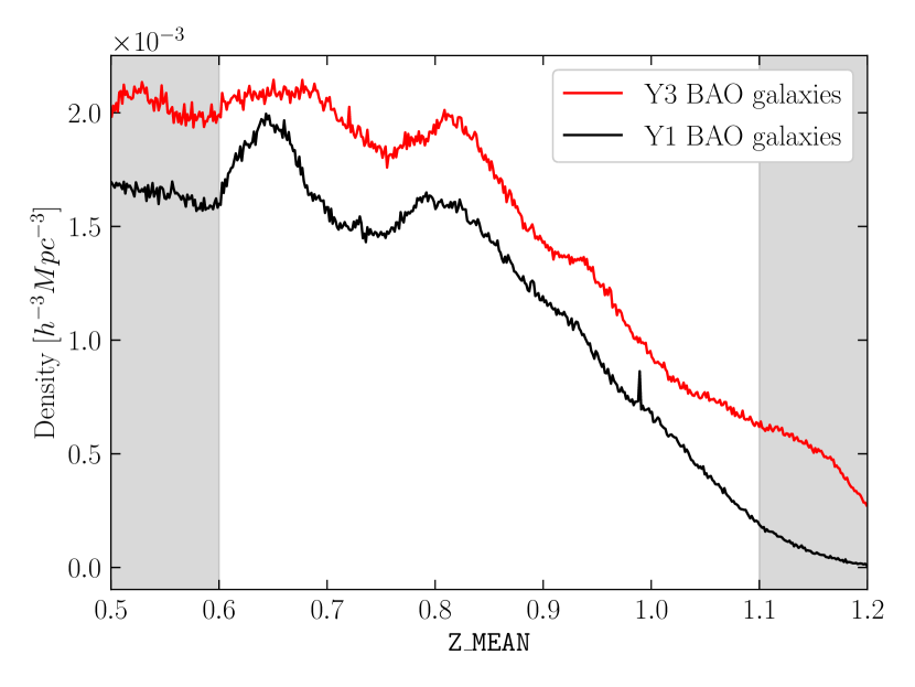
Figure 1: Number density of galaxies found in Y1 GOLD (black) and Y3 GOLD (red). The increase is mostly due to changes in the data reduction process. This increased justified the extension of the galaxy sample to redshift $z=1.1$.

3 Sample selection

The BAO sample has been selected following the same procedure as that of DES Y1 BAO analysis. We first apply the following quality cuts to Y3 GOLD data (Sevilla-Noarbe et al., 2021):

• FLAGS_GOLD: we remove, for all bands $griz$, any source with $\texttt{{FLAGS\_SOF}}\ !=0$, with SourceExtractor $\texttt{{FLAGS}}>3$, or $\texttt{{IMAFLAGS\_ISO}}\ !=0$. As well as any object defined as Bright Blue artifact or Bright objects with nonphysical colors and possible transients.

• FLAGS_FOOTPRINT. We require sources to be defined inside the footprint and to have $\texttt{{NITER\_MODEL\_}}>0$ in all $griz$ bands to ensure that the object has been observed. The footprint is defined as those regions with at least one exposure in all $griz$ bands, with a coincident effective coverage greater than 50% in all bands.

• We further impose sources to be within the angular mask, defined in Section 4.

Once we apply the quality cuts defined above, we select secure galaxies using the EXTENDED_CLASS_MASH_SOF_ classifier, which classifies how much a source differs from a point-like morphology (Sevilla-Noarbe et al., 2021). For photo-$z$ estimates (see Section 5) and for the galaxy colour selection, we use SOF magnitudes corrected by SED-dependent extinction based on SFD98 (Schlegel et al., 1998), chromatic corrections and Y3 GOLD zero-point corrections.

We next apply the colour selection:

$$(i-z)+2\times(r-i)>1.7\ ,$$ (1)

and also the flux-limit cut:

$$i<19.+(3\times\texttt{Z\_MEAN})\ ,$$ (2)

in the magnitude range $17.5<i<22.3$. Finally we select galaxies in the redshift range:

$$0.6<\texttt{Z\_MEAN}<1.1\ .$$ (3)

The flux-limit cut, in the presence of large photo-$z$ scatter, could lead to unwanted correlations with other survey conditions and to an amplification of systematic effects. In our case, the BAO sample is, by definition, designed to avoid large photo-$z$ scatters and therefore, these correlations will be small. Likewise, this effect should be corrected by the amelioration of survey conditions correlations described in Section 8.

Comparing our selection algorithm with the one used for the DES Y1 (see equation 3 in Crocce et al. 2019), we have increased the depth limit up to 22.3$\mathrm{\,mag}$ to reach redshifts $z\leq 1.1$ after considering Equation 2. This, in turn, implies a reduction of an area of 100 square degrees, in comparison with a sample with a depth limit of 22$\mathrm{\,mag}$, reaching redshifts up to $z=1$. Based on cosmological forecasts, adding this extra bin at $z<1.1$ at the expense of losing 100 square degrees results in better constraining power. We predict a gain of 10% in the precision of the BAO scale and a higher mean redshift.

Table 1: Summary of the selection process. Starting from the Y3 GOLD catalogue, we apply the same colour selection as in Y1 GOLD, but we extend the analysis to redshift $z=1.1$. We also need to extend the magnitude limit to $i<22.3$, ensuring completeness through the entire footprint.

Keyword	Cut	Description
Gold	observations present in the Y3 GOLD catalogue	Sevilla-Noarbe et al. (2021)
Quality	FLAGS_GOLD	Section 3
Footprint	4108.47 $deg^{2}$	Section 4
Colour selection	$(i-z)+2\times(r-i)>1.7$	Section 3
Flux Selection	$17.5<i<19.+3.\times\texttt{Z\_MEAN}$	Section 3
Star-galaxy separation	$\texttt{{EXTENDED\_CLASS\_MASH\_SOF\_}}=3$	Section 3
Photo-$z$ range	[$0.6-1.1$]	Section 5

In Table 1, we list all the selections done in the Y3 GOLD sample to select the BAO sample. In Table 2 we summarize the main properties of the BAO sample for each tomographic redshift bin. Redshift properties are explained in Section 5. The galaxy bias estimates of this table have been obtained following the blinding procedure explained in Section 7 and serve as initial values for subsequent analyses.

Table 2: Main properties of the BAO sample in each tomographic bin. Redshift properties are given for the VIPERS sample estimation, namely, the mean redshift ($\bar{z}$), the width of the $N(z)$ ($W_{68}$) and the dispersion on the photo-$z$ error ($\sigma_{68}$). Sample variance are estimated based on MICE simulation. The so-called blind galaxy bias has been obtained following the collaboration’s blinding procedure and serve as initial values needed to mitigate systematic observational effects.

Redshift limits	$\bar{z}$	$W_{68}$	$\sigma_{68}$	Number of galaxies	blind galaxy bias
0.6 < z < 0.7	0.648 $\pm$ 0.003	0.0455 $\pm$ 0.003	0.021 $\pm$ 0.001	1,478,178	1.79 $\pm$ 0.09
0.7 < z < 0.8	0.742 $\pm$ 0.003	0.0522 $\pm$ 0.002	0.025 $\pm$ 0.002	1,632,805	1.83 $\pm$ 0.10
0.8 < z < 0.9	0.843 $\pm$ 0.003	0.0629 $\pm$ 0.003	0.029 $\pm$ 0.002	1,727,646	2.02 $\pm$ 0.12
0.9 < z < 1.0	0.932 $\pm$ 0.004	0.0633 $\pm$ 0.003	0.030 $\pm$ 0.003	1,315,604	2.09 $\pm$ 0.14
1.0 < z < 1.1	1.020 $\pm$ 0.006	0.0808 $\pm$ 0.006	0.040 $\pm$ 0.005	877,760	2.4 $\pm$ 0.08

4 Angular Mask

Apart from the object-to-object selection of the BAO sample, we need to define the effective area of the sample, ensuring we remove areas of dubious quality and that are complete given the magnitude limit of the BAO sample. In DES, the exact image footprint information is delivered as mangle products (Swanson et al., 2008), which are later transformed into HEALPix maps (Górski et al., 2005) of resolution nside =4096. This translation facilitates merging several information maps, which can then be combined to generate the sample’s footprint.

The BAO sample is only defined in the Wide Survey area, excluding the Supernova Fields (see Sevilla-Noarbe et al. 2021 for details). To create the footprint mask, we impose the following requirements in the input HEALPix maps. For details about the maps we refer to Sevilla-Noarbe et al. (2021):

• At least one exposure in each of the $griz$ bands.

• The effective area of each pixel must be greater than 0.8 in $griz$. This cut removes HEALPix pixels lying at the edge of the survey area, or containing significantly masked area.

• Pixels must not be affected by foreground sources, like regions around bright stars or extended galaxies.

• An extra cleaning is done in very obvious pixels affected by scattered light and unmasked streaks.

• Pixel must have a SOF corrected $10\sigma$ depth in $griz$ greater than 22, 22, 22.3, 21$\mathrm{\,mag}$, respectively.

• The depths in $r$ and $z$ bands must follow the condition, $(2\times r_{\mathrm{lim}}-z_{\mathrm{lim}})>24$. This condition is to ensure that our sample selection in Equation (1) remains complete and applicable following the minimum depth cut in $i$-band ($i>22.3$).

After combining all these conditions, we end up with the final BAO sample mask, which covers 4108.47 square degrees. The footprint and density distribution can be seen in Figure 2. Here, the effective area of the pixels are considered. In this figure we also show in red the W1 and W4 VIPERS regions, used for photo-$z$ calibration in Section 5.1.

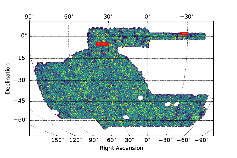
Figure 2: BAO sample angular distribution, covering 4108.47 square degrees of the sky accessible at CTIO. In red squares, VIPERS W1 and W4 regions, used for photo-$z$ validation.

5 Photometric redshifts

Photo-$z$’s used for the BAO sample are derived using the Directional Neighborhood Fitting (DNF) algorithm (De Vicente et al., 2016). We use the photo-$z$ estimates described in Y3 GOLD (Sevilla-Noarbe et al., 2021). In summary, DNF was trained using the most updated spectroscopic sample available for the collaboration by May 2018. This sample contains public spectroscopic but also some DES proprietary spectroscopic data, including the collection from the OzDES collaboration (Lidman et al., 2020). From this sample, we randomly selected half of the objects for training, while the rest was left for general validation purposes. Furthermore, we also removed the whole VIPERS spectroscopic sample from the training sample, and we left it for validation purposes, as explained in the following subsection. To estimate photo-$z$’s, we used SOF corrected fluxes, using $griz$ bands.

In internal analyses, we also tested BPZ code (Benítez, 2000) and Annz2 (Sadeh et al., 2015), but DNF always gave better photo-$z$ bias and $\sigma_{68}$ metrics, and therefore, we use it to estimate redshifts for our BAO sample.

In addition to the predicted best-value in the fitted hyper-plane (Z_MEAN), DNF also returns the redshift of the nearest neighbour (Z_MC). This quantity, stacked for all galaxies in a given tomographic bin, has proven to give a fair description of the true $N(z)$ (Crocce et al., 2019). Likewise, DNF produces redshift probability distributions (PDF) for each source, that can also be used to estimate the $N(z)$ of a given tomographic bin if we stack the PDF of all the selected sources. Both estimates will be used to validate our fiducial $N(z)$, based on the VIPERS spectroscopic survey.

To estimate the $N(z)$ of the BAO sample we use the second public data release (Scodeggio et al., 2018, PDR2) from the “VIMOS Public Extragalactic Redshift Survey” (Guzzo et al., 2014, VIPERS). Unlike with the DES Y1 analysis, where we used the COSMOS sample (Laigle et al., 2016), we employ VIPERS, which is a larger sample and, therefore, less affected by cosmic variance. Likewise, VIPERS is complete up to $i_{AB}\approx 22.5$ for redshifts above 0.5, where the BAO sample is defined.

5.1 VIPERS Validation

The VIPERS sample consists of 91,507 sources, from which 86,775 are galaxies. VIPERS observed in two fields, named W1 and W4, both overlapping DES. W1 is the largest area, centred at ${\alpha_{2000}}=34.495^{\circ}$ and ${\delta_{2000}}=-5.076^{\circ}$, and covers an effective area of 11.012 square degrees, while W4 is centred at ${\alpha_{2000}}=332.7^{\circ}$ and ${\delta_{2000}}=1.61^{\circ}$, and covers 5.312 square degrees. The total overlap area is 16.324 square degrees (seen in Figure 2).

The sample was defined to be statistically complete above redshift 0.5, at least up to $i_{AB}<22.5$ (Scodeggio et al., 2018). Considering that the BAO sample is defined above redshift 0.6 and up to $i_{AB}<22.3$ makes VIPERS an excellent reference sample for the photo-$z$ validation.

As recommended by  Scodeggio et al. (2018), we apply the following quality cuts on the VIPERS data:

• $2\leq zflag<10$: ensures a good quality spectroscopic redshift with more than 90% confidence and eliminates AGNs and duplicated objects.

• The Target Sampling Rate ($tsr$), the Spectroscopic Success Rate ($ssr$) and the Colour Sampling Rate ($csr$) must be greater than zero.

• $classFlag==1$: selects from the main catalog, galaxies with colours compatible with $z>0.5$.

• $photoMask==1$ ensures that galaxies fall within the photometric mask.

These quality cuts are more than sufficient for our analysis, since cosmological constraints coming from the BAO scale measurement are robust against a small number of wrong redshifts in the determination of the $N(z)$.

After applying these cuts, we end up with 74,591 galaxies available for photo-$z$ validation and estimation of our $N(z)$’s. Furthermore, VIPERS statistics must be weighted to account for the various sampling rates. The galaxy weight for each VIPERS galaxy is $w=1./ssr/tsr/csr$.

We then match the VIPERS sample to the BAO sample in separated redshift bins. In total, we have 8362 galaxies matched within 1 $\mathrm{\,arcsec}$, divided into tomographic redshift bins the number of galaxies available for calibration is $1934,~{}2107,~{}2167,~{}1416,~{}738$ respectively. This represents ${\sim}\,12\%$ of the VIPERS galaxy sample. The reduction of the sample comes mostly from the colour selection and the flux selection which by themselves eliminates 82% of the VIPERS catalogue. Despite this reduction, the mean value of $ssr\times tsr\times csr$ in each redshift bin is 0.47, 0.47, 0.45, 0.42, 0.39 respectively, which reflect the completeness of the validation sample with respect to the complete VIPERS sample. We further confirmed the VIPERS sample covers the same colour-colour space as the BAO sample (cf. Appendix A).

We estimate the BAO sample $N(z)$ in each tomographic bin by stacking the VIPERS redshifts for all the matches in the given redshift bin, but before, we validate DNF photo-$z$ point estimates (used to assign galaxies to each tomographic bin) using the VIPERS redshifts (see Section 5.3). The variance in the validation metrics and in the $N(z)$’s are obtained based on $\approx 316$ BAO sample photo-$z$ realizations using the MICE simulation (Fosalba et al., 2015; Crocce et al., 2015), as described in the following subsection.

5.2 Photo-$z$ variance

To estimate the uncertainties of the photo-$z$ metrics and of the $N(z)$’s, we rely on the MICE simulation to create several realizations of the VIPERS-BAO sample. The MICE simulation covers $~{}{\sim}\,5150$ square degrees. Based on the method of Lima et al. (2008), we create a MICE catalogue with the same photometric properties as the Y3 GOLD. From here, we divide the MICE simulation in a total of 316 equal-area sub-samples of 16.3 square degrees, each consisting of two independent regions of 11 and 5.3 square degrees. From here, we select galaxies with the same cuts as in the BAO sample. In each realization, we calculate the $N(z)$ ($316$ $N(z)$ for each redshift bin). Since MICE’s galaxy density is a little higher than VIPERS density, in each of these sub-samples, we randomly pick as many objects as the VIPERS catalogue has, independently for each tomographic bin.

In Appendix A, we show a comparison of the properties of the BAO sample and MICE simulation, confirming the simulation reproduce the photometry of the VIPERS-BAO sample correctly (Figures A.1 and A.2). Hence, we can use MICE to estimate errors of the photo-$z$ metrics and of the $N(z)$’s, as shown in Figures 3, 4, 5 and 6.

5.3 Photo-$z$ validation

We assess the quality of the DNF point photo-$z$ estimates by measuring the photo-$z$ bias and $\sigma_{68}$ in each tomographic bin. These two quantities are the most important ones to estimate the correct angular distance to the BAO. The outlier fraction, a standard metric given when assessing photo-$z$’s in generic studies, does have a negligible effect on BAO measurements, for example.

We then calculate these two metrics for our photo-$z$ choice, based on VIPERS, and also for those estimates based on Z_MC. Z_MC is estimated for each BAO sample source according to its nearest neighbour in the training sample. But the training sample is not constructed to represent the BAO sample and therefore, their metrics are expected to be not as representatives as the VIPERS estimates.

The photo-$z$ bias is defined, averaged over all the available galaxies $N$, as:

$$z_{\mathrm{bias}}=\frac{1}{N}\sum_{i=1}^{N}(\texttt{Z\_MEAN}^{i}-z^{i}_{\mathrm{spec}})$$ (4)

and $\sigma_{68}$ is defined as the value such as 68% of the galaxies have $\lvert\texttt{Z\_MEAN}-z_{\mathrm{spec}}\rvert/(1+z_{\mathrm{spec}})<\sigma_{68}$.

In Figures 3 and 4 we show the evolution of $z_{\mathrm{bias}}$ and $\sigma_{68}$ as a function of $\bar{z}_{\mathrm{spec}}$. Error bars are the sample variance calculated as the standard deviation from the MICE realizations. The level of $\sigma_{68}$ is below 0.1 and the mean bias is below 0.04 in all the redshift ranges, confirming the good quality of the photo-$z$ estimate, as expected by design of the sample selection.

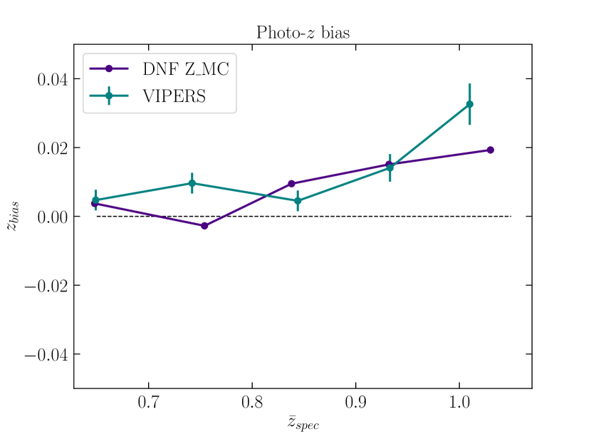
Figure 3: $z_{\mathrm{bias}}$ as a function of $\bar{z}_{\mathrm{spec}}$, for the two $z_{\mathrm{spec}}$ estimates (VIPERS and Z_MC). $z_{\mathrm{bias}}$ is defined as the average difference between Z_MEAN and the given redshift. After finding a good agreement between independent estimates, we assume the VIPERS validation as our default choice. Errors only apply to the VIPERS sample, and they are estimated as the standard deviation from realizations (see Section 5.2).

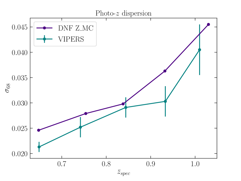
Figure 4: Redshift bias scatter for the two redshift estimates (VIPERS and Z_MC) as a function of $\bar{z}_{\mathrm{spec}}$. $\sigma_{68}$ is defined as the value where 68% of the objects have $\lvert\texttt{Z\_MEAN}-z_{\mathrm{spec}}\rvert/(1+z_{\mathrm{spec}})<\sigma_{68}$.

Once we confirm the quality of the DNF photo-$z$ estimates, we proceed to estimate the true $N(z)$’s in each bin. In Figure 5 we present the $N(z)$ for each tomographic bin estimated with VIPERS, DNF Z_MC and DNF PDF. The variance is obtained based on the standard deviation estimated with MICE simulation. Finally, in Figure 6, we present $W_{68}$, defined as the width containing 68% of the $N(z)$ distribution, and the mean of $N(z)$ as a function of redshift for each calibration sample.

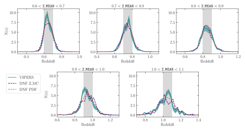
Figure 5: Redshift distributions, $N(z)$, estimated using three different data-sets. We first use DNF Z_MEAN to select galaxies in tomographic bins and then, we estimate the true $N(z)$ using the VIPERS sample. Errors are estimated as the standard deviation from 316 realizations (see Section 5.2). The Z_MC and DNF PDF estimates are only shown for comparison.

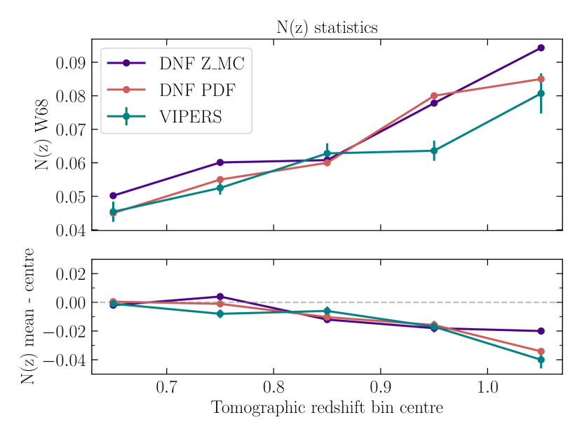
Figure 6: Summary statistics for the $N(z)$ distributions shown in Figure 5. On the top panel, the width of the distribution, $W_{68}$, as a function of the centre of the tomographic redshift bin. $W_{68}$ defines the width containing 68% of the $N(z)$ distribution. On the bottom panel, the difference between the mean of the $N(z)$ and the centre of the bin. Errors only apply to the VIPERS sample, and they are estimated as the standard deviation from 316 mock realizations from MICE (see Section 5.2).

In general, DNF behaves well, confirming Z_MC is a good tracer of the VIPERS redshifts. As already said, several internal tests showed that the choice of one or another $N(z)$ does not change our results.

6 Sample validation

In this section we validate the photometric properties of the BAO sample and estimate the purity of the sample.

6.1 Photometry

The colour selection for the BAO sample was defined to select galaxies beyond $z=0.5$, following the SED for elliptical galaxies. Details about the selection can be found in Figure 5 from Crocce et al. (2019). There we estimated the colours of a set of SED templates as a function of redshift seen through the DES filter passbands. To confirm that the colour selection is still valid for Y3, we run the BAO sample through the SED template fitting code LePhare (Arnouts & Ilbert, 2011), with the same SED templates as in Y1 (Benítez, 2000) and using the most updated versions of the DES filters passbands.

We run LePhare with fixed redshifts to Z_MEAN (we also tested allowing redshifts to vary freely, and results were the same). With the best fitting model for each galaxy, we can examine the proportions of the different spectral type populations within the BAO sample. After running LePhare, we find that 44% of the sample are actually elliptical galaxies, 34% Sbc types, and 22% other types of galaxies. Furthermore, the colours reproduce well the expected locus for each spectral type. This can be seen in Figure 7, where we show the colour evolution of the Elliptical and Sbc galaxies in the BAO sample as a function of redshift. We further show the Y3 GOLD stellar locus for main-sequence stars. This highlights the possible colour confusion between galaxies and stars in our sample in the first redshift bins. Nonetheless, these regimes are where the morphological star/galaxy separation quantity in DES will work better.

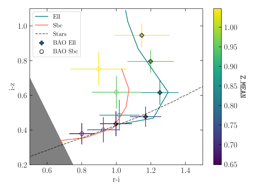
Figure 7: Median colour-colour distributions for the BAO sample, divided into spectral types, as a function of Z_MEAN redshift, compared with the expected colour-colour evolution of Elliptical and Sbc SEDs (solid lines). In dashed line, the Y3 GOLD stellar locus. The white area defines the colour-colour cut applied to select the BAO sample. Error bars are the colour standard deviations of each sub-sample.

6.2 Star contamination

Several studies have shown that star contamination can significantly affect the measurement of clustering of galaxies if not taken care of. On the one hand, they can damp the signal-to-noise ratio of the BAO signal (Carnero et al., 2012), but they can also introduce spurious power at large scales (Ross et al., 2011), which could mimic the effect of primordial non-gaussianities. However, the effect on the angular position of the BAO is negligible. Therefore, some contamination level is allowed, especially since residual stellar contamination in the clustering is removed using the mitigation scheme presented in Section 8.

In this work, as explained in Section 3, we use the EXTENDED_CLASS_MASH_SOF_ classifier to select secure galaxies, which should be a reliable star-galaxy separator in the range of $i=[19,22.5]$, with expected contamination in these magnitude ranges below $2\%$ (Sevilla-Noarbe et al., 2021). Another effect is the possible obscuration of galaxies due to stars in the foreground. This effect is taken care of by the Y3 GOLD foreground mask, which is applied to the BAO sample and should account for the most obscured regions around stars; nonetheless, we can always expect that for low-brightness surface galaxies, this effect might be important, especially as we go to higher redshifts.

We estimate the star contamination level by looking at the purity of the sample, defined as:

$$\mathrm{Purity\ [\%]}=\left(1-\frac{\mathrm{n_{stars}}}{(\mathrm{n_{stars}}+\mathrm{n_{gals}})}\right)\times 100$$ (5)

where $\frac{\mathrm{n_{stars}}}{(\mathrm{n_{stars}}+\mathrm{n_{gals}})}$ is the contamination.

We start by applying the same algorithm as in Y1 (Crocce et al., 2019). There we measured the galaxy density in the BAO sample as a function of stellar density and extrapolate the relation to where stellar density = 0. This way, we can infer the sample purity by looking at the sample density in the absence of stars with respect to the mean density. We do this analysis separately for each tomographic bin to assess the sample’s purity as a function of redshift. The result of this analysis can be found in Figure 8.

The contamination is small but somewhat larger than the average for Y3 GOLD. The highest contamination is found in the second and third bin ($\mathrm{photo-}z\ =[0.7,0.9]$). This is confirmed in Figure 9. Here we show the photo-$z$ distribution if we assume that secure stars are galaxies, given the same colour cut applied to the BAO sample. We can clearly see the distribution peaks in this redshift range. This is because of all stars will colours larger than $r$-$i$ $\gtrsim 1.3$, for which the best photo-$z$ will be that of the galaxies in the turn of the galaxy colour locus ($r$-$i$ $\approx 1.3$, $i$-$z$ $\approx 0.5$, cf. Figure 7). Consequently, for those stars the likelihood of the photo-$z$ fit worsen as they move away of the turn.

The contamination is probably overestimated due to obscuration effects in the borders of field stars. As already commented, this effect might be important in the highest redshift bins, and we see this effect in the last redshift bin ($\mathrm{photo-}z=[1.0,1.1]$). Here we expect very little contamination, but different from the other bins, we see a negative trend in galaxies’ density as a function of stellar density. Internal studies ruled-out the possibility that an over-agressive star-galaxy separation was causing this effect. This warns us that the foreground mask developed for the Y3 GOLD might be insufficient at the faint end and also, that purity might be over-estimated in the second to last redshift bin. Nonetheless, we expect this effect to have a negligible effect on the BAO measurement; likewise, we treat this effect on the mitigation of observing conditions in Section 8.

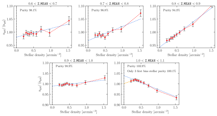
Figure 8: Normalized density versus stellar density (in red). Apart from the last redshift bin, the number of objects in the BAO sample increases with stellar density, expected if we consider contamination by stars. In the last bin, we see the effects of stellar obscuration, and therefore, the purity estimate is not reliable. Nonetheless, it is in this redshift bin where we expect less contamination. In blue, the fit to the distribution. Extrapolating to Stellar density = 0, we can infer the purity of our sample (Equation 5). In the last redshift bin, we also show the linear fit, including only the first three points.

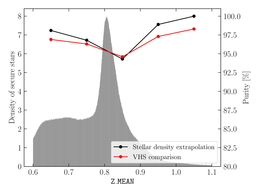
Figure 9: In gray and on the left y-axis, the normalized density of secure stars if they were treated as galaxies that pass the BAO sample colour cut versus DNF photo-$z$. The peak at photo-$z$ $\approx 0.8$ comes from all the stars with colour $r$-$i\gtrsim 1.3$. In lines and on the right y-axis, estimates of galaxy purity by two independent methods as a function of photo-$z$. In black, we show the estimate based on the galaxy density as a function of stellar density, and in red, the purity based on the matched DES-VHS sample. Both estimates agree well and also with the trend seen in the gray distribution.

To confirm our estimates, we further estimate the star contamination by comparing the BAO sample with a different star/galaxy separation scheme, done in a subsample that combines DES photometry with near-infrared (NIR) data. It has been shown in Sevilla-Noarbe et al. (2018) that a combination of optical plus NIR data is excellent to discriminate between stars and galaxies. Therefore we match the BAO sample to the DR4 Vista Hemisphere Survey (McMahon et al., 2013, VHS). The overlap is ${\sim}\,2000$ square degrees, and Our sample contains 987254 of their sources. Unfortunately, VHS is only complete in DES up to $i{\sim}\,21$ so that we can expect some selection bias, especially at high redshifts. We estimate the percentage of stars in the BAO sample following the colour separation seen in Figure 10 from Sevilla-Noarbe et al. (2021). Therefore, we define as stars those sources with $J-Ks<0.2\times(g-i)+0.55$. Applying this cut to each redshift bin in the BAO sample, we find the following purity levels: 96.96%, 96.3%, 94.6%, 97.3%, and 98.3%. They are very similar to the ones found with the previous method, as can be seen in Figure 9. In this case, the incompleteness of VHS at the fainter end is not important because it is here where less contamination is expected.

7 Analysis blinding procedure

To avoid confirmation bias, DES follows strict blinding procedures. In general, we apply the same blinding guidelines for all the LSS samples. Here, the main rule is to avoid the calculation and visual inspection of the angular correlation function, $\omega(\theta)$, or the angular power spectrum before estimating the final cosmological constraints. Clustering statistics are only allowed to be calculated following these rules:

• Clustering measurements for any sample are allowed to be produced for a 10% sub-sample of the area only, in up to 3 angular bins.

• Bias values can be obtained for these measurements, only using the halofit prediction of $\omega(\theta)$ for a fixed cosmology. These bias measurements are only meant to inform either the production of mocks or the forecast to optimized science analysis but not for parameter estimations.

In addition, we apply the blinding rules applied in Y1:

• We cannot over-plot theory and data until the catalogues are frozen and all blinding tests have been approved.

• No maximum likelihood values of any fits to data vectors will be reported until the catalogues are finalized. The width of a confidence interval may be, as well as the shape of the likelihood, as long as it is always centred on a fiducial value.

7.1 Blind galaxy bias

Based on these guidelines, we estimate the galaxy bias for the BAO sample. These values are needed to construct the log-normal mocks used in the mitigation of observational systematic effects explained in Section 8.2.2. We measure $\omega(\theta)$ for 3 angular bins from $\theta{\sim}\,0.58$ to $\theta{\sim}\,0.92$ degrees in a 10% sub-sample, selecting a list of consecutive HEALPix pixels, randomly selected within the footprint, but with preliminary weights defined from the whole footprint. We estimate a Gaussian+shot noise covariance matrix with input $C_{\ell}$ evaluated at MICE $\Lambda$CDM cosmology (Fosalba et al., 2015; Crocce et al., 2015). First, we fit $\omega(\theta)$ with a covariance with galaxy bias $b=1$ in all redshift bins; then, we obtain the first set of temporary galaxy biases that are used to estimate the final covariance matrix. With this new covariance, we obtain the stated galaxy bias per redshift bin. In the process, we include the $N(z)$’s from Section 5 and a first set of weights from the mitigation of systematics (using the Y1 BAO sample bias as starting point). ‘Blind’ galaxy bias values are given in Table 2.

In Figure 10 we compare the BAO sample $\omega(\theta)$ with the average clustering signal from the log-normal mocks (see Section 8.2.2) and the theoretical model with the fitted galaxy biases.

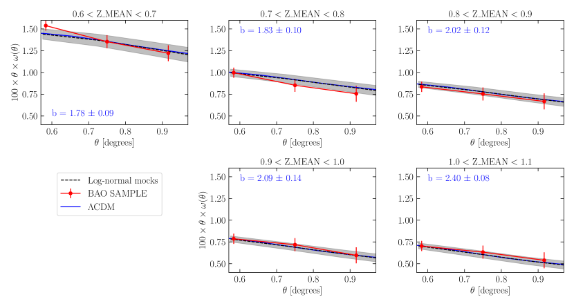
Figure 10: In red is $100\times\theta\times\omega(\theta)$ for the BAO sample. These are the only data points allowed by the blinding procedure to be inspected. These 3 points are used to estimate a “blind galaxy bias” used to construct the log-normal mocks in Section 8.2.2. In blue, the best fit prediction with fixed MICE $\Lambda$CDM cosmology, with $\Omega_{\mathrm{M}}=0.25$, $h=0.7$, $\Omega_{\mathrm{b}}=0.044$ and $n_{\mathrm{s}}=0.95$ (Fosalba et al., 2015). The fit is done using the full covariance between points. In grey, the average $\omega(\theta)$ from the log-normal mocks.

8 Mitigation of Observational Systematic Effects

This paper is based on observations taken during three years of operations at the Blanco telescope in Chile. On average, each position on the sky was observed four times (excluding the Supernova Fields), although the scatter is large, with some regions observed once, with other regions observed up to 10 times (cf. Figure 2 from DES Collaboration 2018). Even though we impose for the BAO sample that we have observed at least once in each band, the heterogeneous survey strategy implies fluctuations in seeing, exposure time, sky brightness, photometric calibrations, and other survey conditions, that, if not treated correctly, can imprint non-cosmological clustering in the density field.

To correct these effects, we apply the iterative decontamination method presented in Elvin-Poole et al. (2018), already applied to the Y1 lensing samples. In Y3, we decided to apply the same methodology to all clustering catalogues, including the BAO sample, redMaGiC (Rozo et al., 2016) and MagLim (Porredon et al., 2021) samples. We have called the method Iterative Systematic Decontamination (ISD) method.

Details about the ISD method and results for the redMaGiC and MagLim  samples are given in Rodríguez-Monroy et al. (2021). In this paper, we explain the methodology and document the results for the BAO sample only.

8.1 ISD Method

The number density of galaxies is expected to fluctuate with the survey’s imaging quality, both due to fluctuations in the noise and due to limitations of the selection process. The method developed in  Elvin-Poole et al. (2018) consists of assessing how much the galaxy density varies with respect to a given survey property, given that the natural variations in number density do not correlate with survey properties. When a significant relationship is found, for example, when the galaxy density increases or decreases with seeing or airmass, a weight is assigned to each galaxy as a function of the observing condition’s value at its position to correct for this fluctuation. In a real case, we have hundreds of survey conditions correlated with each other and for several bands. For this reason, a robust and automatic methodology is needed to correct for observing condition fluctuations.

The ISD method is an iterative method. It starts by estimating the significance of the galaxy density versus each survey property. The method uses HEALPix maps for each survey property as well as to estimate galaxy densities, where we consider the effective area of the pixels given by the Y3 GOLD FOOTPRINT map (Sevilla-Noarbe et al., 2021).

To measure the significance, we start by minimizing $\chi^{2}_{\mathrm{model}}$ for each ith survey property map (SP map), where the model is:

$$\frac{n_{i}}{\langle n\rangle}=m\cdot s_{i}+c\ ,$$ (6)

with $n_{i}$ the number of galaxies as a function of the SP map and $\langle n\rangle$ the average. Finally we estimate a $\Delta\chi^{2}$ as:

$$\Delta\chi^{2}=\chi^{2}_{null}-\chi^{2}_{model}\ ,$$ (7)

between the best-fit linear parameters and a null test with $\frac{n_{i}}{\langle n\rangle}=1$. The covariance used to calculate these $\chi^{2}$ values is given by the dispersion of the same galaxy density - SP map relation measured on the uncontaminated log-normal mocks (see Section 8.2.2).

If $\Delta\chi^{2}$ is actually significant or not, will depend on the noise properties of the sample. Therefore, in order to assess the degree of significance of each SP map, we compare the $\Delta\chi^{2}$ obtained from the data with the probability distribution of $\Delta\chi^{2}$ obtained from a set of galaxy mocks, representing the same numbers, areas, and redshift distributions as the data. From the mocks probability distribution we define $\Delta\chi^{2}(68)$ as the impact degree below which $68\%$ of the $\Delta\chi^{2}$ from the mocks are. Finally, we define the significance of each map SP map as:

$$S_{1D}=\frac{\Delta\chi^{2}}{\Delta\chi^{2}(68)}\ .$$ (8)

The second step is to remove the galaxy density vs survey property relation for a given map by weighting galaxies according to the inverse of the linear relation fit for that map. At each iteration we use the SP map with the highest significance, $S_{1D}$, for this step. Finally, we move to the next iteration, once galaxies have been weighted (corrected).

The method ends when all the $S_{1D}$ are below a given, user pre-defined threshold, $T_{1D}$. The choice of $T_{1D}$ should balance the levels of residual contamination and of over-correction. The final weight is defined as the multiplication of all the weights computed in each iteration and is normalized such that $\langle w\rangle=1$ (average over footprint).

In general, it is not necessarily true that the map to weight for at a given iteration j will be the map with j-th highest $S_{1D}$ at iteration 0, because the existing correlations between SP maps make weighting for a given map to have an effect on others’ significance. This correlation is dealt naturally by the ISD method.

Each iteration step of the ISD method is summarized in Figure 11, given the results for the first redshift bin in the first iteration. On the left, we see the galaxy density as a function of sky-brightness in the $i$-band; as we go to higher sky-brightness regions, the density of galaxies decreases. To assess if this is significant or not, we compare $\Delta\chi^{2}$ from the data to that from 1000 mocks (right-hand side plot). In this case, this relation is the most significant of all the SP maps, and therefore, we will correct the galaxy density by this survey property first and continue to the second iteration.

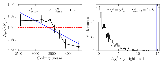
Figure 11: Summary of one iteration in the ISD method. First, we calculate the minimum $\chi^{2}$ value given a linear polynomial fit, and also, by a constant relation. We estimate $\Delta\chi^{2}$ between both and compare it with the probability distribution of $\Delta\chi^{2}$ in a set of mocks. If $\frac{\Delta\chi^{2}}{\Delta\chi^{2}(68)}$ is above a given threshold ($T_{1D}$) and it is the largest from the list of SP maps available, we will use it to create weights following the linear relation found. We repeat this procedure for the remaining maps until all are below $T_{1D}$. In the case of the BAO sample, we chose a $T_{1D}=4$, equivalent to a confidence level $\geq 99\%$.

Recently, other methods have been proposed for the correction of observational systematics in DES Y3 data (Weaverdyck & Huterer, 2021; Rezaie et al., 2020; Wagoner et al., 2021). Moreover, ISD has also been used with alternative configurations, such as using a PCA of the SP maps. A comparison of some of these methods and configurations applied to the REDMAGIC sample is shown in Rodríguez-Monroy et al. (2021). For the BAO sample, none of these methods were available by the time of the freeze of the sample that followed the blinding procedure. The differences between these methods, though small, mostly affect the clustering amplitude but they have a marginal impact on the position of the BAO peak. We checked this impact by comparing the results from our fiducial weights with those from PCA (Rodríguez-Monroy et al., 2021), observing negligible differences.

8.2 Input ingredients

Before running the ISD method, we need to define several inputs. For example, we need to define the threshold $T_{1D}$ below which we demand all SP maps to be below at end of the run. Furthermore, we have assumed a linear fit to model the galaxy density vs. SP map relationship, but nothing prevent us from using higher-order functions. Nonetheless, internal tests have shown that a linear fit is more than sufficient to cope with galaxy density variations for all survey conditions, at least for the level of precision we need for galaxy clustering in the BAO sample. Moreover, higher order fits could lead to over-fitting.

8.2.1 Observing condition maps

DES produces hundreds of observing condition maps for each band in HEALPix format. The definition of these maps are detailed in Sevilla-Noarbe et al. (2021). For convenience, since several of these maps are correlated, we reduce the list to a set of 32 maps (8 in each $griz$ band). Details about the SP maps list reduction is given in Appendix B. Besides, we also create a stellar density map (based on DES morphological classification) and include a galactic extinction map, in this case, the SFD98 map of (Schlegel et al., 1998). Details about the creation of these maps are given in Sevilla-Noarbe et al. (2021). Finally, the list of SP maps used for the BAO sample is (weighted quantities use inverse-variance weights of the single-epoch photometric errors):

• AIRMASS ($griz$): weighted mean airmass from all exposures.

• SKYBRITE ($griz$): weigthed mean sky brightness from all exposures.

• SKYVAR_UNCERT ($griz$): weighted Sky variance with flux scaled by zero point.

• FWHM_FLUXRAD ($griz$): Twice the average half-light radius from the sources used for determining the PSF.

• FGCM_GRY calibration ($griz$): residual ‘grey’ correction to the zero-point.

• SOF_DEPTH ($griz$): galaxy depth at $10\sigma$ for SOF, corrected for zero-points and galactic extinction.

• SIGMA_MAG_ZERO ($griz$): Quadrature sum of zero-point uncertainties.

• T_EFF_EXPTIME ($griz$): exposure time weighted by the effective time of observation.

• STELLAR_DENS: density of stars.

• SFD98: extinction map from Schlegel et al. (1998).

8.2.2 Galaxy mocks

To assess if the density relations in the ISD method are significant or not, we rely on a set of mocks. Given the method’s flexibility, we rely on the log-normal formalism of Coles & Jones (1991) to create a set of 1000 mocks for our analysis. We checked that 1000 mocks were sufficient.

The method is the following: the first step is to log-normalize the real-space $C_{\ell}$’s (see equation 21 in Xavier et al. 2016). After this transformation, $C_{\ell}$’s can be used to create gaussian fields for the matter overdensities. The generated log-normal overdensity maps are then masked and normalized to the input number of galaxies, so the total density is equal to the sample’s density. Finally, we draw random galaxies following a Poissonian distribution to mock the shot-noise on our galaxy sample in the survey masks. The final products of these mocks are HEALPix density maps. We can produce maps in any given resolution. Tests showed that an nside =512 was sufficient without degrading the results.

In our analysis, we run the method twice: first to get a preliminary set of weights that we use to estimate the blind galaxy bias explained in Section 7.1. Using these results, we are able to compute theoretical $C_{\ell}$’s matching the clustering amplitude, that are used both to feed the log-normal mocks and also the COLA mocks in Ferrero et al. (2021). Finally, using the new theoretical $C_{\ell}$’s, we compute 1000 log-normal mocks to feed the mitigation of observational systematics.

Several internal tests showed that changing the fiducial cosmology, $N(z)$, or galaxy biases did not affect the mitigation of systematic effects. This is expected since the general form of the clustering is not important here.

Later in Section 8.4 we will validate the weights over a set of “contaminated” mocks, contaminated with the same observational effects seen in the data. To do so, we will vary the number density according to the BAO sample weights from the same Poisson noise distribution as the “non-contaminated” mocks, therefore, drawing non-contaminated and contaminated mocks from the same random distribution. This is slightly different from the method applied in Rodríguez-Monroy et al. (2021) to the other LSS samples where the “contaminated” mocks are drawn from independent Poisson noise realizations.

8.2.3 Choice of threshold

Unlike the other LSS samples, for the BAO sample, we use a $T_{1D}=4$, equivalent to a confidence level $\geq 99\%$. Our forecasts showed the choice of a strict or loose $T_{1D}$ has almost a negligible effect on BAO measurement (cf. Figure C.1). Therefore, to avoid over-corrections and uncertainties propagation’s in cosmological estimates, we selected a $T_{1D}=4$ as our choice. More details are given in Section 8.4 and Appendix C. Likewise, the mitigation corrections are, at first approximation, flat. Therefore, any remaining systematic not corrected for will be absorbed by the galaxy bias. In the case of BAO measurement, it means that it will have a negligible effect in cosmology, independently of how much we correct. However, some caution must be taken in the case of studying primordial non-gaussianities or other large-scale observables.

8.3 Results for systematic mitigation

We run the ISD method on the BAO sample, with $T_{1D}=4$. In Table 3 we present the maps that we need to correct for in each redshift bin. We find that in most redshift bins, we need to correct by seeing and sky-variance uncertainty, and in some cases, by stellar density. In Figure 12, Figures 13 and 14 we show the ordered list of maps before starting the iterative process, in decreasing order of significance. Also, in these figures, we show the significance level for all SP maps once we stop the process.

BAO sample
photo-$z$ bin	SP maps used to estimate the systematic weights given a tolerance in the method of $T_{1D}=4$
$0.6<z<0.7$	skybrite-i
$0.7<z<0.8$	fwhm_fluxrad-r, fwhm_fluxrad-i, stellar_dens, skyvar_uncert-i
$0.8<z<0.9$	stellar_dens, fwhm_fluxrad-r, fwhm_fluxrad-g,
	fwhm_fluxrad-z, sof_depth-i
$0.9<z<1.0$	skyvar_uncert-r, sfd98, fwhm_fluxrad-g, fwhm_fluxrad-r, airmass-z,
	sof_depth-r, fwhm_fluxrad-z
$1.0<z<1.1$	skyvar_uncert-r, fwhm_fluxrad-i, fwhm_fluxrad-g, stellar_dens,
	fwhm_fluxrad-r, fwhm_fluxrad-z, skyvar_uncert-g, sfd98, airmass_z, t_eff_exptime-z

Table 3: List of SP maps found to have impact on the BAO sample sample at each redshift bin. The rows should be read from left to right in order of importance.

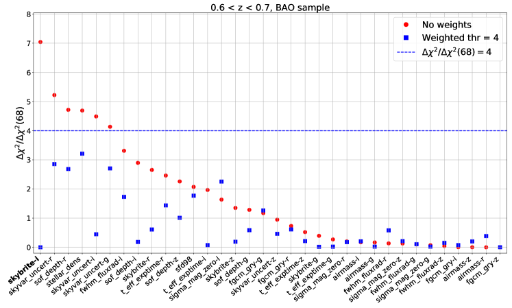
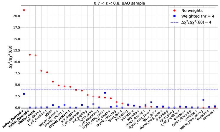
Figure 12: Significance of each SP map with respect to the BAO sample for the first two redshift bins. Figures show the significance of each SP map before starting the method (in red circles) and also, after the method ends once all SP maps are under $T_{1D}=4$ (blue squares). The horizontal dashed line correspond to the significance threshold. The bold labels on the x-axis list the SP maps that have effectively being used to create the final weights.

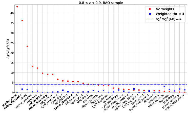
Figure 13: Significance of each SP map with respect to the BAO sample for the third and forth redshift bin. Figures show the significance of each SP map before starting the method (in red circles) and also, after the method ends once all SP maps are under $T_{1D}=4$ (blue squares). The horizontal dashed line correspond to the significance threshold. The bold labels on the x-axis list the SP maps that have effectively being used to create the final weights.

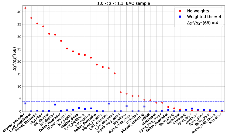
Figure 14: Significance of each SP map with respect to the BAO sample for the last redshift bin. Figures show the significance of each SP map before starting the method (in red circles) and also, after the method ends once all SP maps are under $T_{1D}=4$ (blue squares). The horizontal dashed line correspond to the significance threshold. The bold labels on the x-axis list the SP maps that have effectively being used to create the final weights.

Once we calculate the weights (see Figure 15), we evaluate the impact on $\omega(\theta)$ by measuring the difference before and after applying weights, showed in Figure 15. This comparison follows the blinding procedure described in Section 7. As we move to higher redshifts the correction increases, reaching a level which is several times the statistical error. At the start, this was a puzzling result, and an intense analysis was devoted to optimize the galaxy mask in order to reduce these levels. Still, after eliminating regions with the highest levels of variations in observing conditions, we did not find a significant reduction to propose a decrease in the survey area. In these tests, we concluded it was naturally occurring due to the broad area of the survey and to the larger list of observing conditions with respect to Y1.

At this point is worth noting what happens if we do not correct at all by these effects in cosmological forecasts. In Appendix C we apply the template-based method used by DES (Abbott et al., 2021) to recover the BAO scale, for both contaminated and uncontaminated log-normal mocks. We find that the template-based method is insensitive to these effects and we recover the true BAO scale in both cases. Therefore, the method is robust against the amplitude of the weights. In any case, since the 2-pt statistics (angular correlation function and power spectrum) can be used beyond the estimate of the BAO scale, it is worth applying the weights to measure the unbiased estimates.

Finally, after passing all the validation tests presented in the next section, we conclude the effect is well-characterized and, therefore, not prone to systematic errors beyond the $\omega(\theta)$ statistical error.

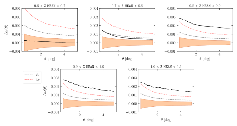
Figure 15: Difference between $\omega(\theta)$ before and after applying the weights, in black. In shaded region, the statistical error calculated as the standard deviation of the 1000 log-normal mocks. In dashed lines the $2\sigma$ and $4\sigma$ error level.

8.4 ISD method validation

We have performed several validation tests on the ISD method, designed to estimate the bias we are introducing in $\omega(\theta)$ after the de-contamination process. More details about the methodology are described in Rodríguez-Monroy et al. (2021). There we validate the methodology for the other LSS samples, using a different list of SP maps (based on principal components). Here we present the results for the BAO sample, using the list of 34 SP maps presented in Section 8.2.1. It is worth noting that we tested the use of the principal components SP maps after unblinding but we did not find any major difference.

These validation tests are run over the mock realizations (the log-normal mocks presented in Section 8.2.2). A negative bias value will mean that we are “over-correcting” $\omega(\theta)$, a positive value that we are not correcting completely. Here we summarize our findings:

• False correction bias: this effect measures the level of bias in $\omega(\theta)$ that we introduce when a chance correlation of a given realization of a SP map correlates with the cosmological structure. For this reason, we run the ISD method on uncontaminated mocks to evaluate how often this occurs, and it depends on the threshold used. A very strict threshold might imply that we will end correcting a spurious correlation. In Figure 16 we show the result for $T_{1D}=4$ and $T_{1D}=2$. In the case of $T_{1D}=2$, we find a bias that for some cases is ${\sim}\,10\%$ the statistical error, while for the case of $T_{1D}=4$, the false correction bias is negligible, justifying the choice of $T_{1D}=4$. These tests are done by applying the ISD method over the “true” un-contaminated mocks.

• Method bias: this effect measures the bias we introduce in $\omega(\theta)$ after correcting for the SP maps defined in the BAO sample, compared to the “true” $\omega(\theta)$. It starts by contaminating the mocks with the same weight found in the data, and then apply the ISD method in each mock, recovering a de-contaminated set of mocks. It is defined as the mean difference between the de-contaminated and the “true” $\omega(\theta)$ from all mocks. We find the method bias to be $\lesssim 10\%$ the statistical error at all scales and redshifts (cf. Figure 17).

• Residual bias: in the method bias, we fixed the list of SP maps used to those found in the data. In the residual bias test, we apply the same method, but this time, without fixing the list of SP maps, i.e.: each mock is free and independent with respect to the SP maps needed. As seen in Figure 18, the bias amplitude reaches ${\sim}\,20\%$ the statistical error in the highest redshift bin, and it is below 10% for the others.

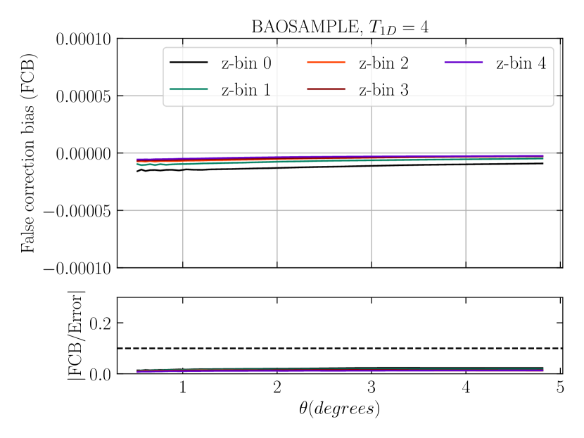
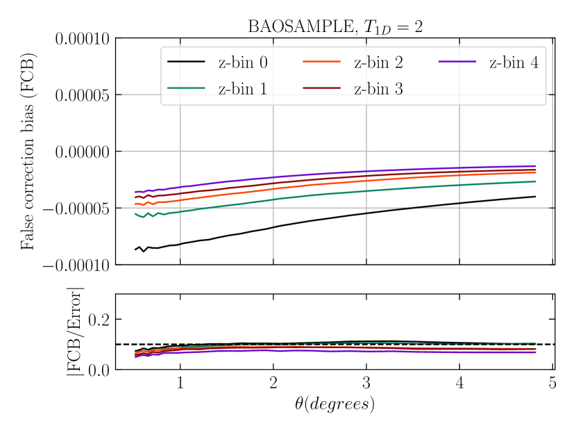
Figure 16: False correction bias for $T_{1D}=4$ (top panel) and $T_{1D}=2$ (bottom panel). It measures the level of bias in $\omega(\theta)$ that might be introduced when we mistake statistical variations in the mocks by a true correlation with the SP maps. We also show the amplitude of the bias with respect to the statistical error. The comparison between different thresholds is one of the arguments used to define $T_{1D}=4$ (equivalent to a confidence level $\geq 99\%$) for the BAO sample. The dashed horizontal line marks the 10% level.

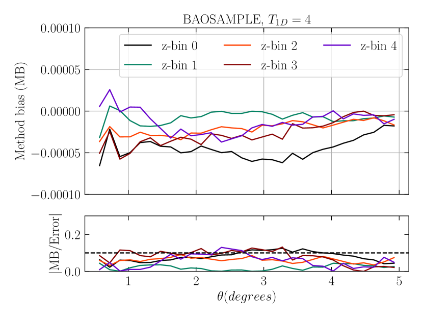
Figure 17: Method bias results, which measure the bias we introduce in $\omega(\theta)$ after correcting for the weights, compared to the “true” $\omega(\theta)$. Bottom plot is the amplitude of the bias with respect to the statistical error. The dashed horizontal line marks the 10% level.

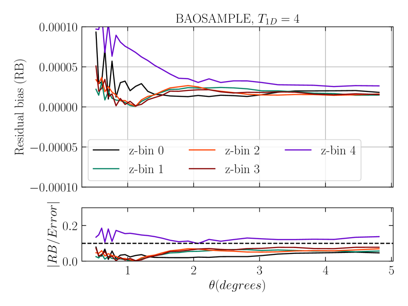
Figure 18: Residual bias for $T_{1D}=4$. In the method bias, we fixed the list of SP maps used to run the method on the contaminated mocks, in the residual bias, we apply the same method, but this time, without choosing a pre-defined list of SP maps to correct for. Bottom plot is the amplitude of the bias with respect to the statistical error. The dashed horizontal line marks the 10% level.

The low level of bias found in all these tests validate the goodness of the method and, even if the correction level is high (as seen in Figure 15) we have demonstrated that the error introduced by the method is always below the statistical one. We conclude that the high correction introduced by observing conditions is due simply to the wide area of the survey, but that there are no pathological issues in the sample.

9 Unblinding $\omega(\theta)$

At this point in the analysis, once we validated the systematic weights and characterized the photo-$z$ distributions, we freeze the BAO sample and prepare for the unblinding of the 2-pt clustering measurements. To do so, we require the BAO sample to pass a series of robustness tests (see Abbott et al. 2021). If all tests are passed, we are ready to unblind the sample and measure the BAO scale. The sample presented in this paper passed all the robustness tests and therefore, it is the base for the BAO distance measurement in DES Y3.

We present the angular correlation function $\omega(\theta)$, split into five redshift bins in Figure 19. These measurements have been obtained using the standard Landy-Szalay estimator (Landy & Szalay, 1993) with CUTE  (Alonso, 2012). Errors in these figures are estimated using the COLA mocks (Ferrero et al., 2021).

In Abbott et al. (2021), the BAO sample is used to estimate the BAO scale at a mean effective redshift of 0.835, both in real and in configuration space, and we calculate the best-fit cosmology to it. Eventually, the BAO scale measurement will also be combined with other DES Y3 cosmological probes to obtain the most precise cosmological constraints from the combination of galaxy clustering and weak lensing.

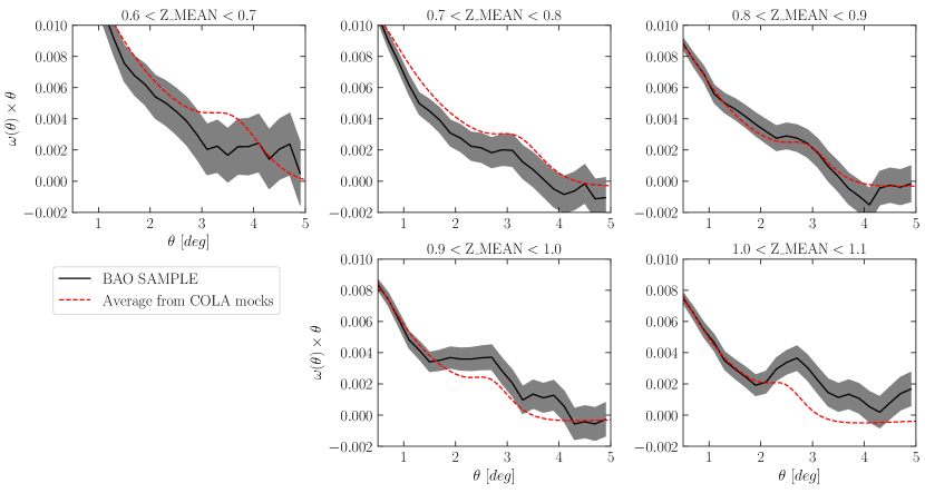
Figure 19: $w(\theta)$ for the 5 tomographic redshift bins (shaded region). Errors are given by the diagonal elements of the covariance matrix coming from the COLA mocks (Ferrero et al., 2021), whose average value is shown in dashed red line. Cosmological implications from the position of the BAO peak are detailed in Abbott et al. (2021).

10 Conclusions

In this paper we describe the data used in DES Y3 for cosmological constraints from the BAO distance scale. Unlike Y1, and thanks to improvements of Y3 data, we have a larger density of galaxies that allows the extension of the analysis to redshift 1.1, increasing the effective redshift of the sample from 0.81 to 0.835. The sample covers 4100 square degrees to a depth of $i_{AB}\leq 22.3$ for galaxies with signal-to-noise greater than $10\sigma$. The galaxy selection is done based on the same colour scheme applied in Y1. This selection ensures a good photo-$z$ estimate, as attested by our photo-$z$ validation for galaxies with photo-$z$ $>0.5$. Also, good quality photo-$z$’s ensure the $N(z)$ of the samples are well characterized. In the Y3 sample, we mitigate spurious clustering that arises from observing conditions with the same methodology used in the Y1 lensing samples. These weights are later applied to the BAO sample in order to obtain un-biased angular correlation functions and power spectra. Cosmological implications of these results are later discussed in Abbott et al. (2021).

Data availability

A general description of DES data releases is available on the survey website at https://www.darkenergysurvey.org/the-des-project/data-access/. BAO sample is available on the DES Data Management website hosted by the National Center for Supercomputing Applications at https://des.ncsa.illinois.edu/releases/y3a2.

11 Affiliations

¹ Instituto de Astrofísica de Canarias, E-38205 La Laguna, Tenerife, Spain
² Universidad de La Laguna, Dpto. Astrofísica, E-38206 La Laguna, Tenerife, Spain
³ Laboratório Interinstitucional de e-Astronomia - LIneA, Rua Gal. José Cristino 77, Rio de Janeiro, RJ - 20921-400, Brazil
⁴ Centro de Investigaciones Energéticas, Medioambientales y Tecnológicas (CIEMAT), Madrid, Spain
⁵ Institut d’Estudis Espacials de Catalunya (IEEC), 08034 Barcelona, Spain
⁶ Institute of Space Sciences (ICE, CSIC), Campus UAB, Carrer de Can Magrans, s/n, 08193 Barcelona, Spain
⁷ Center for Cosmology and Astro-Particle Physics, The Ohio State University, Columbus, OH 43210, USA
⁸ Department of Physics, The Ohio State University, Columbus, OH 43210, USA
⁹ Institute of Theoretical Astrophysics, University of Oslo. P.O. Box 1029 Blindern, NO-0315 Oslo, Norway
¹⁰ Physics Department, 2320 Chamberlin Hall, University of Wisconsin-Madison, 1150 University Avenue Madison, WI 53706-1390
¹¹ Department of Physics, University of Michigan, Ann Arbor, MI 48109, USA
¹² Instituto de Física Teórica, Universidade Estadual Paulista, São Paulo, Brazil
¹³ Instituto de Física Teórica UAM/CSIC, Universidad Autónoma de Madrid, 28049 Madrid, Spain
¹⁴ Departamento de Física Teórica, Facultad de Ciencias, Universidad Autónoma de Madrid, E-28049 Cantoblanco, Madrid, Spain
¹⁵ Instituto de Física Gleb Wataghin, Universidade Estadual de Campinas, 13083-859, Campinas, SP, Brazil
¹⁶ Jet Propulsion Laboratory, California Institute of Technology, 4800 Oak Grove Dr., Pasadena, CA 91109, USA
¹⁷ Kavli Institute for Particle Astrophysics & Cosmology, P. O. Box 2450, Stanford University, Stanford, CA 94305, USA
¹⁸ ICTP South American Institute for Fundamental Research, Instituto de Física Teórica, Universidade Estadual Paulista, São Paulo, Brazil
¹⁹ Department of Astronomy, University of Geneva, ch. d’Écogia 16, CH-1290 Versoix, Switzerland
²⁰ Cerro Tololo Inter-American Observatory, NSF’s National Optical-Infrared Astronomy Research Laboratory, Casilla 603, La Serena, Chile
²¹ Fermi National Accelerator Laboratory, P. O. Box 500, Batavia, IL 60510, USA",0000-0002-7069-7857
²² CNRS, UMR 7095, Institut d’Astrophysique de Paris, F-75014, Paris, France
²³ Sorbonne Universités, UPMC Univ Paris 06, UMR 7095, Institut d’Astrophysique de Paris, F-75014, Paris, France
²⁴ Department of Physics & Astronomy, University College London, Gower Street, London, WC1E 6BT, UK
²⁵ Department of Astronomy and Astrophysics, University of Chicago, Chicago, IL 60637, USA
²⁶ SLAC National Accelerator Laboratory, Menlo Park, CA 94025, USA
²⁷ School of Mathematics and Physics, University of Queensland, Brisbane, QLD 4072, Australia
²⁸ INAF, Astrophysical Observatory of Turin, I-10025 Pino Torinese, Italy
²⁹ Center for Astrophysical Surveys, National Center for Supercomputing Applications, 1205 West Clark St., Urbana, IL 61801, USA
³⁰ Department of Astronomy, University of Illinois at Urbana-Champaign, 1002 W. Green Street, Urbana, IL 61801, USA
³¹ Institut de Física d’Altes Energies (IFAE), The Barcelona Institute of Science and Technology, Campus UAB, 08193 Bellaterra (Barcelona) Spain
³² Jodrell Bank Center for Astrophysics, School of Physics and Astronomy, University of Manchester, Oxford Road, Manchester, M13 9PL, UK
³³ University of Nottingham, School of Physics and Astronomy, Nottingham NG7 2RD, UK
³⁴ Astronomy Unit, Department of Physics, University of Trieste, via Tiepolo 11, I-34131 Trieste, Italy
³⁵ INAF, Observatorio Astronomico di Trieste, via G. B. Tiepolo 11, I-34143 Trieste, Italy
³⁶ Institute for Fundamental Physics of the Universe, Via Beirut 2, 34014 Trieste, Italy
³⁷ Observatório Nacional, Rua Gal. José Cristino 77, Rio de Janeiro, RJ - 20921-400, Brazil
³⁸ School of Mathematics and Physics, University of Queensland, Brisbane, QLD 4072, Australia
³⁹ Department of Physics, IIT Hyderabad, Kandi, Telangana 502285, India
⁴⁰ Kavli Institute for Cosmological Physics, University of Chicago, Chicago, IL 60637, USA
⁴¹ Department of Physics and Astronomy, University of Pennsylvania, Philadelphia, PA 19104, USA
⁴² Santa Cruz Institute for Particle Physics, Santa Cruz, CA 95064, USA
⁴³ Department of Astronomy, University of Michigan, Ann Arbor, MI 48109, USA
⁴⁴ Institute of Astronomy, University of Cambridge, Madingley Road, Cambridge CB3 0HA, UK
⁴⁵ Kavli Institute for Cosmology, University of Cambridge, Madingley Road, Cambridge CB3 0HA, UK
⁴⁶ Centre for Astrophysics & Supercomputing, Swinburne University of Technology, Victoria 3122, Australia
⁴⁷ Faculty of Physics, Ludwig-Maximilians-Universit"̈at, Scheinerstr. 1, 81679 Munich, Germany
⁴⁸ Center for Astrophysics $|$ Harvard & Smithsonian, 60 Garden Street, Cambridge, MA 02138, USA
⁴⁹ Lawrence Berkeley National Laboratory, 1 Cyclotron Road, Berkeley, CA 94720, USA
⁵⁰ Department of Astronomy/Steward Observatory, University of Arizona, 933 North Cherry Avenue, Tucson, AZ 85721-0065, USA
⁵¹ Australian Astronomical Optics, Macquarie University, North Ryde, NSW 2113, Australia
⁵² Lowell Observatory, 1400 Mars Hill Rd, Flagstaff, AZ 86001, USA
⁵³ Sydney Institute for Astronomy, School of Physics, A28, The University of Sydney, NSW 2006, Australia
⁵⁴ Centre for Gravitational Astrophysics, College of Science, The Australian National University, ACT 2601, Australia
⁵⁵ The Research School of Astronomy and Astrophysics, Australian National University, ACT 2601, Australia
⁵⁶ Departamento de Física Matemática, Instituto de Física, Universidade de São Paulo, CP 66318, São Paulo, SP, 05314-970, Brazil
⁵⁷ George P. and Cynthia Woods Mitchell Institute for Fundamental Physics and Astronomy, and Department of Physics and Astronomy, Texas A&M University, College Station, TX 77843, USA
⁵⁸ Institució Catalana de Recerca i Estudis Avançats, E-08010 Barcelona, Spain
⁵⁹ Max Planck Institute for Extraterrestrial Physics, Giessenbachstrasse, 85748 Garching, Germany
⁶⁰ Université Clermont Auvergne, CNRS/IN2P3, LPC, F-63000 Clermont-Ferrand, France
⁶¹ Department of Physics and Astronomy, University of Waterloo, 200 University Ave W, Waterloo, ON N2L 3G1, Canada
⁶² Perimeter Institute for Theoretical Physics, 31 Caroline St. North, Waterloo, ON N2L 2Y5, Canada
⁶³ Department of Astrophysical Sciences, Princeton University, Peyton Hall, Princeton, NJ 08544, USA
⁶⁴ Brookhaven National Laboratory, Bldg 510, Upton, NY 11973, USA
⁶⁵ School of Physics and Astronomy, University of Southampton, Southampton, SO17 1BJ, UK
⁶⁶ Computer Science and Mathematics Division, Oak Ridge National Laboratory, Oak Ridge, TN 37831
⁶⁷ Institute of Cosmology and Gravitation, University of Portsmouth, Portsmouth, PO1 3FX, UK
⁶⁸ Department of Physics, Stanford University, 382 Via Pueblo Mall, Stanford, CA 94305, USA
⁶⁹ McDonald Observatory, The University of Texas at Austin, Fort Davis, TX 79734

Appendix A MICE photometric validation

In Section 5.2 we measured the standard deviation of our $N(z)$’s by comparing the BAO sample-VIPERS distribution to that from several realizations of the MICE simulation. To do so, we must be certain that the photometric properties of the MICE simulation match those from VIPERS and the BAO sample.

In this Appendix we show the photometric comparisons between the BAO sample and the MICE mocks. In Figure A.1 we show the magnitude distribution of the samples in $griz$. In Figure A.2 we show the comparison in colour-colour space.

The photometric properties of MICE, BAO sample and VIPERS are very similar, hence, we can use this simulation to estimate errors in our $N(z)$’s.

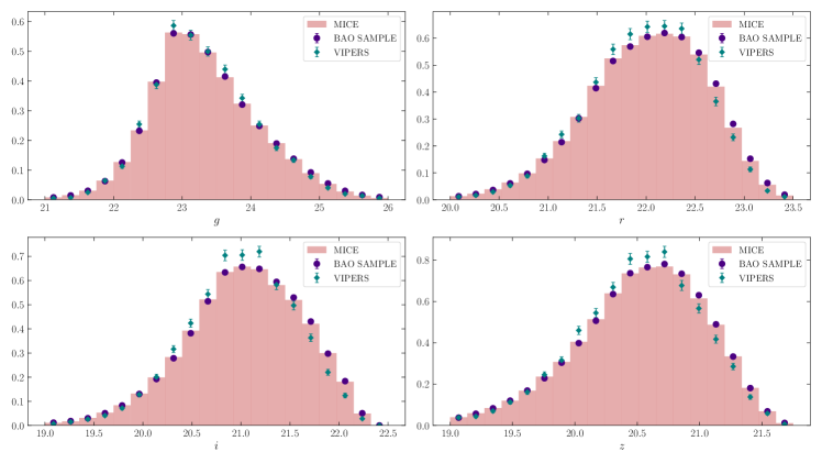
Figure A.1: Normalized distribution of the magnitudes in the different bands (top left: $g$, top right: $r$, bottom left: $i$, bottom right: $z$). Blue histogram: MICE data, orange points: DES data, green points: VIPERS data.

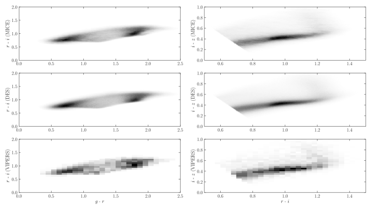
Figure A.2: Color-color distribution $g-r$ vs $r-i$ for MICE (top left panel), BAO sample (middle left panel) and VIPERS (bottom left panel). Color-color distribution $r-i$ vs $i-z$ for MICE (top right panel), BAO sample (middle right panel) and VIPERS (bottom right panel).

Appendix B Selection of representative SP maps

As explained in Section 8, ISD is an iterative process that evaluates the significance of each SP map at each redshift bin of the BAO sample. Moreover, the 1D relations are calculated on a set of 1000 log-normal mocks, also at each redshift bin. This leads to a huge amount of computing time. For this reason, in order to optimize the iterative process that we applied to decontaminate the data, we reduce the number of SP maps that the pipeline has to run over. For this purpose, we look at their Pearson’s correlation coefficients and set a lower limit $r_{l}$ for them. This way, we identify groups of highly correlated SP maps by looking at those maps with $\lvert r_{P}\rvert\geq r_{l}$ (cf. Figure B.1).

To check the stability of these groups with respect to the selection of $r_{l}$, we evaluate the correlation matrix ranging the value of $r_{l}$ from $0.5$ to $0.9$. Below $r_{l}=0.5$ many SP maps are considered correlated (in the extreme case of a very low $r_{l}$ the whole matrix is considered a single group, so in that case an alternative would be to perform a PCA of the SP maps), while above $r_{l}=0.9$ most of the maps are considered independent (there are almost no off-diagonal elements), not allowing us to reduce the number of maps, as desired. We observe a stable group structure between $r_{l}=0.5$ and $0.7$, finally taking the highest value as our limit. Once we identify the SP map groups from the correlation matrix, we select a representative map from each of them. The representative SP maps chosen are listed in Section 8.2.1.

We use the weighted average SP maps in all cases with the exception of the zero point residues, for which we use the total SP maps. To further ensure the stability of our results under the choice of these representative maps, we run ISD with slightly different lists of representative maps using different statistics within each SP map group. Since the number of maps needed to weight for is similar in all cases, we conclude that our results are stable under this choice. Furthermore, we apply this process for each photometric band separately, and we check that the same list of representative SP maps works for the four of them.

In Figure B.2 we show the correlation matrix for the final representative SP maps in $i$-band and the correlation of these sets of maps in the four bands that we work with, respectively. The remaining correlations at the same photometric band or among them are finally dealt by the correction pipeline.

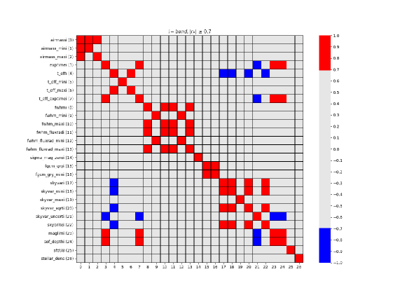
Figure B.1: Pearson’s correlation matrix for the $i$-band SP maps. Red (blue) cells correspond to the SP map pairs with correlation coefficient higher (lower) than $r_{l}=0.7$. This helps us not only to identify SP map groups formed by the different statistics of the same observing condition, but also correlations among maps out of these groups, as for example the expected correlation between depth and exposure time.

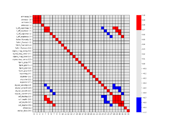
Figure B.2: Correlation matrix for the representative SP maps in all photometric bands. The structures are similar equivalent to those seen in the case of individual photometric bands.

Appendix C Effect of weighting in BAO measurement

We run forecasts on BAO measurement using the log-normal mocks, applying a template-based method to recover the BAO scale (Seo et al., 2012; Xu et al., 2012; Anderson et al., 2014; Ross et al., 2017). This method estimates how different the BAO position is with respect to an assumed template cosmology. The difference is encoded in the parameter $\alpha$, which re-scales the separation between the BAO scale position in the theory and observation.

We run it for uncontaminated mocks (without any systematic effect), in contaminated mocks with weights obtained at $T_{1D}=2$, and also, for de-contaminated mocks after applying the ISD scheme with $T_{1D}=4$ on the previous mocks, i.e., with a more relaxed threshold than the input contamination. The summary of this test can be found in Figure C.1. Interestingly, we find the measurement works very well independent of whether we correct or not for observational systematics, as well as for the decontaminated mocks. In Table C.1 we show the recovered $\alpha$ in each case. This result is due to the fact that the contamination in the $\omega(\theta)$ is flat and does not affect the BAO scale. This finding is another argument to select the $T_{1D}=4$ in the analysis, instead of $T_{1D}=2$.

Table C.1: Mean $\alpha$ value and standard deviation from 1000 mocks. We recover the true cosmology in all cases and with the same precision. $\alpha$ encodes the BAO scale position difference between observations and theory.

	uncontaminated	contaminated	decontaminated
$\bar{\alpha}\pm\ std$	$1.01\pm 0.02$	$1.01\pm 0.02$	$1.01\pm 0.02$

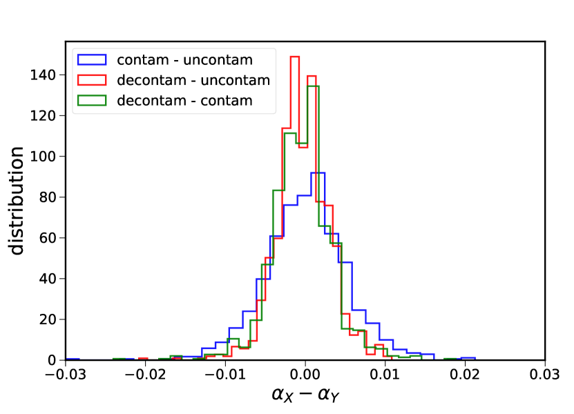
Figure C.1: Difference in $\alpha$ found in three sets of mocks: uncontam are uncontaminated mocks, with no systematic effects. contam are the same mocks, contaminated with weights obtained at $T_{1D}=2$ and decontam are the same contaminated mocks, after applying the ISD method at $T_{1D}=4$. The differences are compatible, confirming that the effect of weighting is small in BAO measurement.

References

- Abbott et al. (2019) Abbott T. M. C., et al., 2019, MNRAS, 483, 4866
- Abbott et al. (2021) Abbott T. M. C., et al., 2021, Dark Energy Survey Year 3 Results: A 2.7% measurement of Baryon Acoustic Oscillation distance scale at redshift 0.835 (arXiv:2107.04646)
- Alam et al. (2017) Alam S., et al., 2017, MNRAS, 470, 2617
- Alonso (2012) Alonso D., 2012, arXiv e-prints, p. arXiv:1210.1833
- Anderson et al. (2014) Anderson L., et al., 2014, MNRAS, 441, 24
- Arnouts & Ilbert (2011) Arnouts S., Ilbert O., 2011, LePHARE: Photometric Analysis for Redshift Estimate, Astrophysics Source Code Library (ascl:1108.009)
- Ata et al. (2018) Ata M., et al., 2018, MNRAS, 473, 4773
- Bautista et al. (2017) Bautista J. E., et al., 2017, A&A, 603, A12
- Benítez (2000) Benítez N., 2000, ApJ, 536, 571
- Beutler et al. (2011) Beutler F., et al., 2011, MNRAS, 416, 3017
- Blake et al. (2011) Blake C., et al., 2011, MNRAS, 415, 2892
- Bond & Efstathiou (1984) Bond J. R., Efstathiou G., 1984, ApJ, 285, L45
- Bond & Efstathiou (1987) Bond J. R., Efstathiou G., 1987, MNRAS, 226, 655
- Burke et al. (2018) Burke D. L., et al., 2018, AJ, 155, 41
- Carnero et al. (2012) Carnero A., Sánchez E., Crocce M., Cabré A., Gaztañaga E., 2012, MNRAS, 419, 1689
- Cole et al. (2005) Cole S., et al., 2005, MNRAS, 362, 505
- Coles & Jones (1991) Coles P., Jones B., 1991, Monthly Notices of the Royal Astronomical Society, 248, 1
- Crocce et al. (2011) Crocce M., Gaztañaga E., Cabré A., Carnero A., Sánchez E., 2011, MNRAS, 417, 2577
- Crocce et al. (2015) Crocce M., Castander F. J., Gaztañaga E., Fosalba P., Carretero J., 2015, Monthly Notices of the Royal Astronomical Society, 453, 1513
- Crocce et al. (2019) Crocce M., et al., 2019, Monthly Notices of the Royal Astronomical Society, 482, 2807
- DES Collaboration (2016) DES Collaboration 2016, MNRAS, 460, 1270
- DES Collaboration (2018) DES Collaboration 2018, ApJS, 239, 18
- De Vicente et al. (2016) De Vicente J., Sánchez E., Sevilla-Noarbe I., 2016, MNRAS, 459, 3078
- Drlica-Wagner et al. (2018) Drlica-Wagner A., et al., 2018, ApJS, 235
- Eisenstein et al. (2001) Eisenstein D. J., et al., 2001, AJ, 122, 2267
- Eisenstein et al. (2005) Eisenstein D. J., et al., 2005, ApJ, 633, 560
- Elvin-Poole et al. (2018) Elvin-Poole J., et al., 2018, Phys. Rev. D, 98, 042006
- Estrada et al. (2009) Estrada J., Sefusatti E., Frieman J. A., 2009, ApJ, 692, 265
- Ferrero et al. (2021) Ferrero I., et al., 2021, Dark Energy Survey Year 3 Results: Galaxy mock catalogs for BAO analysis (arXiv:2107.04602)
- Flaugher (2005) Flaugher B., 2005, International Journal of Modern Physics A, 20, 3121
- Flaugher et al. (2015) Flaugher B., Diehl H. T., Honscheid K., et al., 2015, AJ, 150, 150
- Fosalba et al. (2015) Fosalba P., Crocce M., Gaztañaga E., Castander F. J., 2015, MNRAS, 448, 2987
- Gaztañaga et al. (2009) Gaztañaga E., Cabré A., Hui L., 2009, MNRAS, 399, 1663
- Górski et al. (2005) Górski K. M., Hivon E., Banday A. J., Wandelt B. D., Hansen F. K., Reinecke M., Bartelmann M., 2005, ApJ, 622, 759
- Gschwend et al. (2018) Gschwend J., et al., 2018, Astronomy and Computing, 25, 58
- Guzzo et al. (2014) Guzzo L., et al., 2014, A&A, 566, A108
- Hütsi (2010) Hütsi G., 2010, MNRAS, 401, 2477
- Kitanidis et al. (2020) Kitanidis E., et al., 2020, Monthly Notices of the Royal Astronomical Society, 496, 2262
- Laigle et al. (2016) Laigle C., et al., 2016, ApJS, 224, 24
- Landy & Szalay (1993) Landy S. D., Szalay A. S., 1993, ApJ, 412, 64
- Laurent et al. (2017) Laurent P., et al., 2017, Journal of Cosmology and Astroparticle Physics, 2017, 017
- Li et al. (2016a) Li T. S., DePoy D. L., Marshall J. L., Tucker D., Kessler R., Annis J., et al., 2016a, AJ, 151, 157
- Li et al. (2016b) Li T. S., et al., 2016b, The Astronomical Journal, 151, 157
- Lidman et al. (2020) Lidman C., et al., 2020, MNRAS, 496, 19
- Lima et al. (2008) Lima M., Cunha C. E., Oyaizu H., Frieman J., Lin H., Sheldon E. S., 2008, MNRAS, 390, 118
- McMahon et al. (2013) McMahon R. G., Banerji M., Gonzalez E., Koposov S. E., Bejar V. J., Lodieu N., Rebolo R., VHS Collaboration 2013, The Messenger, 154, 35
- Morganson et al. (2018) Morganson E., et al., 2018, Publications of the Astronomical Society of the Pacific, 130, 074501
- Padmanabhan et al. (2007) Padmanabhan N., et al., 2007, MNRAS, 378, 852
- Peebles & Yu (1970) Peebles P. J. E., Yu J. T., 1970, ApJ, 162, 815
- Percival et al. (2007) Percival W. J., Cole S., Eisenstein D. J., Nichol R. C., Peacock J. A., Pope A. C., Szalay A. S., 2007, MNRAS, 381, 1053
- Percival et al. (2010) Percival W. J., et al., 2010, MNRAS, 401, 2148
- Porredon et al. (2021) Porredon A., et al., 2021, Phys. Rev. D, 103, 043503
- Rezaie et al. (2020) Rezaie M., Seo H.-J., Ross A. J., Bunescu R. C., 2020, MNRAS, 495, 1613
- Rodríguez-Monroy et al. (2021) Rodríguez-Monroy M., et al., 2021, Dark Energy Survey Year 3 Results: Galaxy clustering and systematics treatment for lens galaxy samples (arXiv:2105.13540)
- Ross et al. (2011) Ross A. J., et al., 2011, MNRAS, 417, 1350
- Ross et al. (2015) Ross A. J., Samushia L., Howlett C., Percival W. J., Burden A., Manera M., 2015, MNRAS, 449, 835
- Ross et al. (2017) Ross A. J., et al., 2017, MNRAS, 464, 1168
- Ross et al. (2020) Ross A. J., et al., 2020, MNRAS, 498, 2354
- Rozo et al. (2016) Rozo E., et al., 2016, MNRAS, 461, 1431
- Sadeh et al. (2015) Sadeh I., Abdalla F. B., Lahav O., 2015, preprint, (arXiv:1507.00490)
- Schlegel et al. (1998) Schlegel D. J., Finkbeiner D. P., Davis M., 1998, ApJ, 500, 525
- Scodeggio et al. (2018) Scodeggio M., et al., 2018, A&A, 609, A84
- Seo et al. (2012) Seo H.-J., et al., 2012, The Astrophysical Journal, 761, 13
- Sevilla-Noarbe et al. (2018) Sevilla-Noarbe I., et al., 2018, MNRAS, 481, 5451
- Sevilla-Noarbe et al. (2021) Sevilla-Noarbe I., et al., 2021, ApJS, 254, 24
- Sunyaev & Zeldovich (1970) Sunyaev R. A., Zeldovich Y. B., 1970, Ap&SS, 7, 3
- Swanson et al. (2008) Swanson M. E. C., Tegmark M., Hamilton A. J. S., Hill J. C., 2008, MNRAS, 387, 1391
- Vakili et al. (2019) Vakili M., et al., 2019, MNRAS, 487, 3715
- Wagoner et al. (2021) Wagoner E. L., Rozo E., Fang X., Crocce M., Elvin-Poole J., Weaverdyck N., Collaboration) D., 2021, Monthly Notices of the Royal Astronomical Society, 503, 4349
- Weaverdyck & Huterer (2021) Weaverdyck N., Huterer D., 2021, MNRAS, 503, 5061
- Xavier et al. (2016) Xavier H. S., Abdalla F. B., Joachimi B., 2016, MNRAS, 459, 3693
- Xu et al. (2012) Xu X., Padmanabhan N., Eisenstein D. J., Mehta K. T., Cuesta A. J., 2012, MNRAS, 427, 2146
- Zhou et al. (2020) Zhou R., et al., 2020, Research Notes of the American Astronomical Society, 4, 181