Continuous Time Bandits With Sampling Costs

Abstract

We consider a continuous time multi-arm bandit problem (CTMAB), where the learner can sample arms any number of times in a given interval and obtain a random reward from each sample, however, increasing the frequency of sampling incurs an additive penalty/cost. Thus, there is a tradeoff between obtaining large reward and incurring sampling cost as a function of the sampling frequency. The goal is to design a learning algorithm that minimizes the regret, that is defined as the difference of the payoff of the oracle policy and that of the learning algorithm. We establish lower bounds on the regret achievable with any algorithm, and propose algorithms that achieve the lower bound up to logarithmic factors. For the single arm case, we show that the lower bound on the regret is $\Omega(1/\mu)$, and an upper bound with regret $O((\log(T/\lambda))^{2}/\mu)$, where $\mu$ is the mean of the arm, $T$ is the time horizon, and $\lambda$ is the tradeoff parameter between the payoff and the sampling cost. With $K$ arms, we show that the lower bound on the regret is $\Omega(K\mu[1]/\Delta^{2})$, and an upper bound $O(K(\log(T/\lambda))^{2}\mu[1]/\Delta^{2})$ where $\mu[1]$ now represents the mean of the best arm, and $\Delta$ is the difference of the mean of the best and the second-best arm.

1 Introduction

The classical discrete-time multi-arm bandit (DMAB) is a versatile learning problem Bubeck et al. (2012); Lattimore and Szepesvári (2019) that has been extensively studied in literature. By discrete-time, we mean that there are a total of $T$ discrete slots, and in each slot, a learning algorithm can choose to ‘play’ any one of the possible $K$ arms.

In this paper, we consider a continuous-time multi-arm bandit problem (CTMAB) that is well motivated from pertinent applications discussed later in this section. In particular, in CTMAB, the total time horizon is $T$, and there are $K$ arms. The main distinction between the DMAB and the CTMAB is that with the CTMAB, an arm can be sampled/played at any (continuous) time $t$ before $T$. Once the sampling time $t\in[0,T]$ is selected, similar to the DMAB problem, any one of $K$ arms can be played, and if arm $k$ is played at time $t$, the learning algorithm gets a random reward with mean $\mu[k]$ independent of the time $t$. Without loss of generality, we let $1>\mu[1]>\mu[2]\dots>\mu[K]$.

Without any other restriction, per se, any algorithm can play infinite number of arms in time horizon $T$ by repeatedly playing arms at arbitrarily small intervals. Thus, to make the problem meaningful, we account for the sampling (arm playing) cost that depends on how often any arm is sampled. Specifically, if two consecutive plays (of any two arms) are made at time $t$ and $t+\Delta t$, then the sampling cost for interval $\Delta t$ is $f(\Delta t)$, where $f$ is a decreasing function. The total sampling cost is defined as the sum of sampling cost over the total time horizon $T$. Sampling cost penalizes high frequency sampling i.e., the higher the frequency of consecutive plays, the higher is the sampling cost. Considering sampling cost depending on consecutive plays of a specific arm results in multiple decoupled single arm CTMAB problems, thus a special case of the considered problem.

The overall payoff in CTMAB is then defined as the accumulated random reward obtained from each sample minus $\lambda$ times the total sampling cost over the time horizon $T$. The variable $\lambda$ represents the relative weight of the two costs. The regret is defined as usual, the expected difference between the overall payoff of the oracle policy and that of a learning algorithm. There is a natural tradeoff in CTMAB, higher frequency sampling increases the accumulated reward but also increases the sampling cost at the same time. Compared to DMAB, where an algorithm has to decide which arm to play next at each discrete time, in CTMAB, there are two decisions to be made, given the history of decisions and the current payoff (reward minus the sampling cost); i) which arm to play next, and ii) at what time.

We next discuss some practical motivations for considering the CTMAB. We first motivate the CTMAB in the single arm case ($K=1$) which in itself is non-trivial. Consider that there is a single agent (human/machine) that processes same types of jobs (e.g. working in call center, data entry operation, sorting/classification job etc.) with an inherent random quality of work $q$, and random per-job (unknown) utility $u(q)$. The agent demands a payment depending on how frequently it is asked to accomplish a job Gong and Shroff (2019). Alternatively, as argued in Gopalakrishnan et al. (2016), the quality of agents’ work suffers depending on the speed of operation/load experienced. Thus, the payoff is the total accumulated utility minus the payment or the speed penalty (that depends on the frequency of work), and the objective is to find the optimal speed of operation, to maximize the overall payoff.

To motivate the CTMAB with multiple arms, the natural extension of this model is to consider a platform or aggregator that has multiple agents, each having a random work quality and corresponding per-job utility. The random utility of any agent can be estimated by assigning jobs to it and observing its outputs. The platform charges a cost depending on the speed (frequency) of job arrivals to the platform, that is indifferent to the actual choice of the agent being requested for processing a particular job. Given a large number of jobs to be processed in a finite time, the objective is to maximize the overall payoff; the total accumulated utility minus the payment made to the platform. When the platform cost is the sum of the cost across agents, where each agent cost depends on the rate at which it processes jobs, the problem decouples into multiple single arm CTMAB problems.

In this paper, for the ease of exposition, we assume that the sampling cost function $f$ is $f(x)=\frac{1}{x}$, i.e., if two consecutive plays are made at time $t$ and $t+\Delta t$, then the sampling cost for interval $\Delta t$ is $\frac{1}{\Delta t}$, which is intuitively appealing and satisfies natural constraints on $f$. How to extend results for general functions is discussed in Remark 21. Under this sampling cost function, assuming arm $1$ has the highest mean $\mu[1]$, it turns out (Proposition 2) that the oracle policy always plays the best arm (arm with the highest mean) $N^{\star}_{T}=\Theta\left(\mu[1]T/\lambda\right)$ times at equal intervals in interval $[0,T]$. Importantly, the number of samples (or sampling frequency) obtained by the oracle policy depends on the mean of the best arm.

This dependence of the oracle policy’s choice of the sampling frequency on the mean of the best arm results in two main distinguishing features of the CTMAB compared to the DMAB problem, described as follows. CTMAB is non-trivial even when there is only a single arm unlike the DMAB problem, where it is trivial. The non-triviality arises since the learning algorithm for the CTMAB has to choose the time at which to obtain the next sample that depends on the mean of that arm, which is also unknown. Moreover with CTMAB, it is not enough to identify the optimal arm, the quality of the estimates is equally important as the sampling cost depends on that. In contrast, with DMAB, it is sufficient for an algorithm to identify the right ordering of the arms.

Recall that we have assumed $\mu[1]<1$. The case $\mu[k]\geq 1$ will follow similarly, where it is worth noting that the setting of $\mu[k]\geq 1$ is easier than when $\mu[1]<1$, since estimates of $\mu[1]$ have to be accurately estimated in CTMAB, and that becomes harder as $\mu[1]$ decreases.

Our contributions for the CTMAB are as follows.

1. For the single arm CTMAB, where $\mu=\mu[1]$, we propose an algorithm whose regret is at most $O\left(\frac{1}{\mu}(\log(T/\lambda))^{2}\right)$. In converse, we show that for any online algorithm that uses only unbiased estimators of $\mu$ for making its decisions, its regret is $\Omega\left(\frac{1}{\mu}\right)$. The reason for considering the unbiased restriction is that the sample mean has the minimum variance among all unbiased estimators of the true mean, a fact critically exploited in the proof.

Thus, as a function of $\mu$, the proposed algorithm has the optimal regret, while there is a logarithmic gap in terms of $T/\lambda$. The result has an intuitive appeal since as $\mu<1$ decreases, the regret increases, since for the CTMAB, $\mu$ has to be estimated, and that becomes harder as $\mu$ decreases.

2. For the general CTMAB with multiple arms, we propose an algorithm whose regret is at most $O\left(\frac{\mu[1]K\log^{2}(T/\lambda)}{\Delta^{2}}\right)$ when $\frac{K}{\mu[1]}=O\left(\frac{\mu[1]}{\Delta^{2}}\right)$, which is a practically reasonable regime. The derived results holds more generally and not just for $\frac{K}{\mu[1]}=O\left(\frac{\mu[1]}{\Delta^{2}}\right)$. In converse, we show that for any online algorithm its regret is $\Omega\left(\frac{K\mu[1]}{\Delta^{2}}\right)$ when $\Delta$ is small. To derive this lower bound we do not need the assumption that an online algorithm uses only unbiased estimators of $\mu[k],k=1,\dots,K$ for making its decisions since we are able to exploit the fact that there are multiple arms and an algorithm has to identify the best arm. Similar to the single arm case, as a function of $\mu[1]$ and $\Delta$, the proposed algorithm has the optimal regret, while there is a logarithmic gap in terms of $T/\lambda$.

1.1 Related Works

In prior work, various cost models have been considered for the bandit learning problems. The cost could be related to the consumption of limited resources, operational, or quality of information required.

Cost of resources: In many applications (e.g., routing, scheduling) resource could be consumed as actions are applied. Various models have been explored to study learning under limited resources or cost constraints. The authors in Badanidiyuru et al. (2018) introduce Bandits with Knapsack that combines online learning with integer programming for learning under constraints. This setting has been extended to various other settings like linear contextual bandits Agrawal and Devanur (2016), combinatorial semi-bandits Abinav and Slivkins (2018), adversarial setting Immorlica et al. (2019), cascading bandits Zhou et al. (2018). The authors in Combes et al. (2015) establish lower bound for budgeted bandits and develop algorithms with matching upper bounds. The case where the cost is not fixed but can vary is studied in Ding et al. (2013).

Switching Cost: Another set of works study Bandit with Switching Costs where cost is incurred when learner switches from one arm to another arm Dekel et al. (2014); Cesa-Bianchi et al. (2013). The extension to the case where partial information about the arms is available through feedback graph is studied in Arora et al. (2019). For a detailed survey on bandits with switching cost we refer to Jun (2004).

Information cost: In many applications the quality of information acquired depends on the associated costs (e.g., crowd-sourcing, advertising). While there is no bound on the cost incurred in these settings, the goal is to learn optimal action incurring minimum cost. Hanawal et al. (2015b, a) trade-offs cost and information in linear bandits exploiting the smoothness properties of the rewards. Several works consider the problem of arm selection in online settings (e.g., Trapeznikov and Saligrama (2013); Seldin et al. (2014)) involving costs in acquiring labels Zolghadr et al. (2013).

Variants of bandits problems where rewards of arm are delay-dependent are studied in Cella and Cesa-Bianchi (2020); Pike-Burke and Grunewalder (2019); Kleinberg and Immorlica (2018). In these works, the mean reward of each arm is characterized as some unknown function of time. These setups differ from the CTMAB problem considered in this paper, as they deal with discrete time setup, and do not capture the cost associated with sampling rate of arms. Rested and restless bandit setups Whittle (1988) consider that distribution of each arm changes in each round or when it is played, but do not assign any penalty on rate of sampling.

In this work, our cost accounting is different from the above referenced prior work. The cost is related to how frequently the information/reward is collected. Higher the frequency, higher is the cost. Also, unlike the DMAB problem, there is no limit on the number of samples collected in a given time interval, however, increasing the sampling frequency also increases the cost.

A multi-arm bandit problem, where pulling an arm excludes the pulling of any arm in future for a random amount of time (called delay) similar to our inter-sampling time has been considered in György et al. (2007). However, in György et al. (2007) the delay experienced (inter-sampling time) is an exogenous random variable, while it is a decision variable in our setup. Moreover, the problem considered in György et al. (2007) is trivial with a single arm similar to the usual DMAB, while it is non-trivial in our case as accuracy of the mean estimates play a crucial role.

2 The Model

There are a total of $K$ arms and the total time horizon is $T$. At any time $t\in[0,T]$, any one of the arms can be played/sampled. On sampling arm $i$ at any time $t$, a random binary reward $X_{i}$ is obtained which follows a Bernoulli distribution with mean $\mu[i]$. We consider Bernoulli distribution here, however, all results will hold for bounded distributions. If the time difference between any two consecutive samples is $\Delta t$, then the sampling cost for interval $\Delta t$ is $f(\Delta t)=1/\Delta t$. We make this choice for $f$ to keep the exposition simple, and more general convex functions can be analysed similarly, see Remark 21. The learning algorithm is aware of $T$. More discussion on this assumption is provided in Remark 10. The ordered arms are denoted by $\mu[1]>\cdots>\mu[K]$, where $\mu[1]<1$.

Let the consecutive instants at which any arm is sampled by a learning algorithm, denoted as $\mathcal{A}$, be $t_{0},t_{1},t_{2},\dots,$ where $t_{0}=0$, and the inter-sampling time be $\Delta t_{i}=t_{i}-t_{i-1}$. Let $k(t_{i})$ denote the arm sampled at time $t_{i}$. Then the instantaneous expected payoff of $\mathcal{A}$ from the $i^{th}$ sample is given as ${\mathsf{p}}_{i}=\mathbb{E}\left[X_{k(t_{i})}\right]-\lambda f(\Delta t_{i})=\mu_{k(t_{i})}-\frac{\lambda}{\Delta t_{i}}$, where $\lambda$ is the trade-off parameter between the sampling cost and the reward. The cumulative expected payoff of the algorithm $\mathcal{A}$ is given by

$$P_{\mathcal{A}}(T)=\sum_{i=1}^{N_{T}}{\mathsf{p}}_{i},$$ (1)

where $N_{T}$ is the total number of samples obtained by $\mathcal{A}$ over the horizon $T$. Whenever necessary we also write $P_{\mathcal{A}}(T)$ as $P_{\mathcal{A}}([0,T])$ to specify the interval over which the payoff is being computed.

The oracle policy that knows the mean values $\mu[k],k=1,\dots,K,$ always samples the best arm $\mu[1]$.

Proposition 1

If $N$ samples are obtained in time $[0,t]$ at times $t_{i}$ with $\Delta t_{i}=t_{i}-t_{i-1}$, then the cumulative sampling cost $\sum_{i=1}^{N}\frac{1}{\Delta t_{i}}$ over time horizon $[0,t]$, where $\sum_{j=1}^{N}\Delta t_{i}\leq t,$ is minimized if the $N$ samples are obtained at equal intervals in $[0,t]$ for any $t$, i.e., $\Delta t_{i}=T/N$ $\forall\ i$.

Proof of Proposition 1 is immediate by noticing that $1/x$ is a convex function, and the fact that for a convex function $f$, $x^{\star}_{i}=1/n,\ \forall\ i=1,\dots,n$ is the optimal solution to $\min_{x_{i}}\sum_{i=1}^{n}f(x_{i}),\ \text{such that}$ $\ x_{i}\geq 0$, and $\sum_{i=1}^{n}x_{i}\leq 1.$ Using Proposition 1, we have that the payoff of the oracle policy is

$$P^{\star}(T) =\max_{N^{o}_{T}}\mu[1]N^{o}_{T}-\frac{N^{o}_{T}\lambda}{T/N^{o}_{T}}=\max_{N^{o}_{T}}\mu[1]N^{o}_{T}-\frac{(N^{o}_{T})^{2}\lambda}{T},$$ (2)

where $N^{o}_{T}$ samples are obtained in total by the oracle policy. Directly optimizing (2) over $N^{o}_{T}$, we obtain that the optimal number of samples obtained by the oracle policy and the corresponding optimal payoff is given by Proposition 2, assuming $\frac{\mu[1]T}{2\lambda}$ to be an integer.

Proposition 2

The oracle policy always samples arm $1$, $N^{\star}_{T}=\frac{\mu[1]T}{2\lambda}$ times in time horizon $[0,T]$ at equal intervals, i.e., at uniform frequency of $N^{\star}_{T}/T$. With $N^{\star}_{T}=\frac{\mu[1]T}{2\lambda}$, the optimal payoff (2) is given by $P^{\star}(T)=\frac{\mu[1]^{2}T}{4\lambda}.$

Note that the sampling frequency $N^{\star}_{T}/T$ of the oracle policy depends on the mean of the best arm, which distinguishes the CTMAB from the well studied DMAB.

Remark 3

For fixed $\mu[1],\dots,\mu[K]$, CTMAB problem with parameters $(\lambda,T)$ is equivalent to CTMAB problem with parameters $(c\lambda,cT)$ where $c>0$ is a constant. To see this, if $\Delta t_{i}$ is the sampling duration with parameters $(\lambda,T)$, then using $c\Delta t_{i}$ as the sampling duration with parameters $(c\lambda,cT)$ results in the same payoff. Thus, $\frac{T}{\lambda}$ is an invariant of the considered problem, and for notational simplicity from here on we just write $T$ to mean $\frac{T}{\lambda}$.

The regret for an algorithm $\mathcal{A}$ is defined as

$$\mathcal{R}_{A}(T)=P^{\star}(T)-P_{\mathcal{A}}(T),$$ (3)

and the objective of the algorithm is to minimize $\mathcal{R}_{A}(T)$. We begin our discussion on the CTMAB problem by considering the case when there is only a single arm, which as discussed before is a non-trivial problem.

3 CTMAB with A Single Arm

In this section, we consider the CTMAB, when there is only a single arm with true mean $\mu$, and $\mu<1$. Results when $\mu>1$ can be obtained by using appropriate scaling similar to the usual DMAB problem. With the single arm, we denote the binary random reward obtained by sampling at time $t_{i}$ as $X_{i}$, and ${\mathbb{E}}\{X_{i}\}=\mu,\ \forall\ i$.

3.1 Algorithm CTSAB

In this section, we propose an algorithm that achieves a regret within logarithmic terms of the lower bound derived in Theorem 7.

Algorithm CTSAB: Divide the total time horizon $[0,T]$ in two periods: learning and exploit. Pick $0<\epsilon<1$. The algorithm works in phases, where phase $1$ starts at time $0$ and ends at time $T^{\epsilon}$. Subsequently, phase $i$, $2\leq i\leq i^{\star}$ ($i^{\star}$ is defined in (5)) starts at time $T^{(i-1)\epsilon}$ and ends at $T^{i\epsilon}$ with duration $T^{i\epsilon}-T^{(i-1)\epsilon}$. For each phase $i$, $1\leq i\leq i^{\star}$, the algorithm obtains $N_{i}=\kappa\log(T)T^{2/3i\epsilon}$ samples in phase $i$ equally spaced in time, i.e., at uniform frequency in that phase. At the end of phase $i$, the total number of samples obtained is $N^{i}=\sum_{j\leq i}N_{j}$, and let

$${\hat{\mu}}_{i}=\frac{1}{N^{i}}\sum_{k=1}^{N^{i}}X_{k},$$ (4)

be the empirical average of all the sample rewards obtained until the end of phase $i$.

The absolute difference between the empirical average and the true mean is defined as err.

Remark 4

With abuse of notation, we interchangeably use $\text{err}_{N},\text{err}_{i},\text{err}_{t}$ to denote the error after $N$ samples or after phase $i$ or at time $t$. Thus, the error in estimating $\mu$ at the end of phase $i$ is $\text{err}_{i}=|{\hat{\mu}}_{i}-\mu|$.

We next define $i^{\star}$, and the algorithm to follow after phase $i^{\star}$. For a given $\delta$ (input to the algorithm), let $i^{\star}$ be the earliest phase at which

$$\sqrt{\frac{\log(2/\delta)}{N^{i^{\star}}}}<\frac{{\hat{\mu}}_{i^{\star}}}{2},$$ (5)

where $N^{i^{\star}}=\sum_{j\leq i^{\star}}N_{j}$. If no such $i^{\star}$ is found, then we define that the algorithm fails.

The learning period ends at phase $i^{\star}$, and the exploit period starts from the next phase $i^{\star}+1$. Each phase $i>i^{\star}$ is of the same time duration $T^{i^{\star}\epsilon}$ till the total time horizon $T$ is reached. Starting from phase $i^{\star}+1$ and for all subsequent phases $k\geq i^{\star}+1$, the algorithm assumes ${\hat{\mu}}_{k-1}$ (4) to be the true value of $\mu$, and obtains $N_{k}=\frac{{\hat{\mu}_{k-1}}T^{i^{\star}\epsilon}}{2}$ samples in phase $k$, equally spaced in time, and ${\hat{\mu}_{k}}$ is updated at the end of each phase $k\geq i^{\star}+1$ using all the samples obtained so far since time $t=0$. The pseudo code for the algorithm is given in Algorithm 1 (presented in supplementary material).

The proposed algorithm CTSAB follows the usual approach of exploration and exploitation, however, there are two non-trivial problems being addressed, whose high level idea is as follows. The aim of the learning period is to obtain sufficient number of samples $N$, such that $\text{err}_{N}<\mu$. Since otherwise, the payoff obtained in phases after the learning period cannot be guaranteed to be positive, following Lemma 19. So the first problem is a stopping problem, checking for $\text{err}_{N}<\mu$, which is non-trivial, since $\mu$ is unknown. For this purpose, a surrogate condition (5) is defined, and the learning period is terminated as soon as (5) is satisfied for a particular choice of $\delta$. Choosing $\delta=\frac{1}{T^{2}}$, using Corollary 12 and Lemma 15, we show that whenever (5) is satisfied, $\text{err}_{N}<\mu$ with probability at least $1-\delta$.

The second problem remaining is to bound the time by which the learning period ends, i.e., (5) is satisfied. We need this bound since non-zero payoff can be guaranteed only for phases that belong to the exploit period that starts after the learning period. Towards that end, we show that the length of learning period is $O(T^{p^{\star}+\epsilon})$ with high probability in Lemma 13, where $p^{\star}$ is defined as follows.

$$T^{p^{\star}}=\frac{1}{\mu^{3}}\ \text{for}\ 0\leq p^{\star}\leq 1.$$ (6)

This automatically means that we are assuming that the time horizon $T$ is at least as large as $\frac{1}{\mu^{3}}$. The lower bound on regret in Theorem 7 implies that $T=o(\frac{1}{\mu^{3}})$ is a degenerate regime for the studied problem. The main result of this subsection is as follows.

Theorem 5

The expected regret of algorithm CTSAB while choosing $\delta=\frac{1}{T^{2}}$ is

$$O(\mu^{2}T^{p^{\star}+(4/3)\epsilon}\log(2T^{2})\log(2T))(1-\frac{1}{T^{1+\epsilon}})+\frac{\mu^{2}}{4}\left(\frac{1}{T^{\epsilon}}+\frac{1}{T}\right),$$

for any $\epsilon>0$, where $p^{\star}$ as defined in (6).

All missing proofs can be found in the supplementary material. Given that $T$ is fixed and $\epsilon>0$ is a variable, we choose $\epsilon$ such that $T^{\epsilon}$ is a constant. With this choice, since $\mu<1$, using (6) the regret bound of the CTSAB algorithm (Theorem 5) is $O\left(\frac{(\log(T)^{2}}{\mu}\right)$, that differs from the lower bound to be derived in Theorem 7 only by logarithmic terms.

3.2 Lower Bound

For deriving the lower bound in the single arm case, we consider only those algorithms that satisfy the following assumption.

Assumption 6

For any online algorithm for the single arm CTMAB problem maximizing (1), the decision variables are the sampling times $t_{i}^{\prime}$s. We consider only those online algorithms that at any time make these decisions depending on an unbiased estimate of $\mu$.

Theorem 7

Let $\mu<1/4$. Let the regret of any online algorithm for the single arm CTMAB for which Assumption 6 holds be $g(\mu,T)$. Let $g(\mu,T)$ be expressed as $g(\mu,T)=\mu^{2}T^{p}$ for some $p<1$. Then $p$ must satisfy, $p\geq\min\{p_{1},p_{2}\},$ where

$$T^{p_{1}}\geq\frac{{\mathsf{c}}_{1}}{\mu^{3}}\ \ \text{for}\ \ 0\leq p_{1}\leq 1,\quad\text{and}$$ (7)

$$p_{2}=\min\left\{k\geq 0:\frac{1}{T^{k}}\left(\frac{{\mathsf{c}}_{2}}{\mu^{2}}\right)^{2}=\max\left\{\mu^{2}T^{k},\frac{{\mathsf{c}}_{3}}{\mu}\right\}\right\},$$ (8)

where ${\mathsf{c}}_{1},{\mathsf{c}}_{2},{\mathsf{c}}_{3}$ are constants.

Thus, $p_{1}$ and $p_{2}$ satisfy $T^{p_{1}}=\Omega\left(\frac{1}{\mu^{3}}\right)$ and $T^{p_{2}}=\Omega\left(\frac{1}{\mu^{3}}\right)$, and the regret of any online algorithm satisfying Assumption 6 is $g(\mu,T)=\mu^{2}T^{p}=\Omega\left(\frac{1}{\mu}\right)$.

The main idea to prove Theorem 7 is detailed in Appendix F. Comparing Theorem 5 and Theorem 7, we see that algorithm CTSAB achieves optimal regret up to logarithmic factors of $T$.

4 CTMAB with Multiple Arms

In this section, we consider the general CTMAB problem with $K$ arms that have means $1>\mu[1]>\cdots>\mu[K]$ and $\Delta=\mu[1]-\mu[2]>0$, and the objective is to minimize the regret defined in (3).

4.1 Upper Bound - Algorithm CTMAB

We propose an algorithm for the CTMAB problem, called the CTMAB algorithm, that is neither aware of $\Delta$ or the actual means $\mu[k]$, and show that its regret is within logarithmic terms of the lower bound (Theorem 9). The first part of the algorithm is called the estimation period, that is designed to estimate the mean $\mu[1]$ of the best arm within an error of at most $\mu[1]$ with high probability. The estimation period of algorithm CTMAB is equivalent to the learning period of algorithm CTSAB applied simultaneously to all the $K$ arms.

Similar to algorithm CTSAB’s learning period, the estimation period of algorithm CTMAB ends as soon as the condition $\sqrt{\frac{\log(2/\delta)}{N^{t}[k]}}<\frac{{\hat{\mu}}_{t}[k]}{2}$ is satisfied for some arm $k\in\{1,\dots,K\}$, where $N^{t}[k]$ is the number of samples obtained for arm $k$ by time $t$, and ${\hat{\mu}}_{t}[k]$ is the empirical average of the sample rewards for arm $k$ with $N^{t}[k]$ samples. If this condition is not satisfied at all, we define that the algorithm fails. Note that the estimation period is not trying to identify the best arm, but the objective is to just estimate the mean of the best arm within an error of $\mu[1]$. In particular, we will show that with high probability whenever the algorithm does not fail, $\frac{2}{3}\mu[1]\leq{\hat{\mu}}_{t}[a_{t}]\leq 2\mu[1]$, where ${\hat{\mu}}_{t}[a_{t}]$ is the estimate of $\mu[1]$ output by the algorithm.

Once the estimation period is over, the identification period begins that is used to identify the best arm with high probability. Using the estimate ${\hat{\mu}}[1]$ of the mean of the best arm $\mu[1]$ found in the estimation period, in the identification period, the best arm is identified using the LUCB1 algorithm Kalyanakrishnan et al. (2012), where samples are obtained at speed one sample per $1/{\hat{\mu}}[1]$ time. The speed choice is required to be dependent on $\mu[1]$ to keep the regret low, and that is why we need the estimation period to get a ‘good’ estimate of $\mu[1]$. Once the identification period ends (where the best arm is identified with high probability), the final period called exploit begins that only considers the arm identified in the identification period as the best, and executes the exploit period of algorithm CTSAB. The pseudo code for algorithm CTMAB is provided in Algorithm 2 (presented in the supplementary material).

The main result of this subsection is as follows.

Theorem 8

With the choice of $\delta=\frac{1}{T^{2}}$, the expected regret of the CTMAB algorithm is at most

$$O\left(\max\left\{\frac{\mu[1]K}{\Delta^{2}}\log T,\frac{K^{2}}{\mu[1]}\log^{2}T,\frac{\log^{2}T}{\mu[1]}\right\}\right)$$

$$\cdot\left(1-\frac{1}{T^{1+\nu_{m}}}\right)\left(1-\frac{1}{T^{2}}\right)$$

$$\quad+O(T)\left(1-\left(1-\frac{1}{T^{1+\nu_{m}}}\right)\left(1-\frac{1}{T^{2}}\right)\right)$$

where $T^{\nu_{m}}$ is the width of each phase after the identification period is over.

With $\frac{K}{\mu[1]}=O(\frac{\mu[1]}{\Delta^{2}})$ (which is a reasonable setting since $K$ is typically not too large), the regret of the CTMAB algorithm is $O\left(\frac{K\mu[1](\log(T))^{2}}{\Delta^{2}}\right)$ matching the lower bound to be derived in Theorem 9 upto logarithmic terms.

The basic idea to derive Theorem 8 is as follows. In Lemma 13 we show that for the truly best arm, arm $1$, the condition $\sqrt{\frac{\log(2/\delta)}{N^{t}[1]}}<\frac{{\hat{\mu}}_{t}[1]}{2}$ is satisfied by time at most $O(T^{p^{\star}+\epsilon})$ with probability at least $1-1/T^{2}$, where $T^{\epsilon}$ is a constant and $p^{\star}$ is as defined in (6) with $\mu[1]=\mu$. Thus, the estimation phase terminates by time $O(T^{p^{\star}})$ with probability at least $1-1/T^{2}$. Moreover, we show in Lemma 22, that whenever the estimation phase terminates, the estimated mean ${\hat{\mu}}[a_{t}]$ satisfies $|{\hat{\mu}}[a_{t}]-\mu[1]|\leq\frac{\mu[1]}{2}$ with high probability. Consequently, we show that the payoff of the estimation period is at least $-O\left(\frac{K^{2}\log^{2}T}{\mu[1]}\right)$ with high probability as shown in Lemma 23.

From Kalyanakrishnan et al. (2012)[Thm 6], we know that the LUCB1 algorithm needs $O\left(\frac{K\log T}{\Delta^{2}}\right)$ expected samples to identify the best arm with high probability (setting $\epsilon=0$ and $\delta=1/T$). Thus, by obtaining these samples at a frequency of one sample per $1/({\hat{\mu}}[1])$ time in the identification period, where $|{\hat{\mu}}[1]-\mu[1]|\leq\mu[1]$ is guaranteed, the total time needed for the identification period is $O\left(\frac{K\log(T)}{\Delta^{2}\mu[1]}\right)$ with high probability. The choice of the frequency of obtaining samples in the identification period needs to depend on $\mu[1]$ to keep the regret of the identification period small. With this choice of sampling frequency, the payoff of the identification period is at most $-O\left(\frac{4K}{\mu[1]\Delta^{2}}\log\left(T^{2}\right)\right)$ as shown in (31) with high probability.

Once the identification period ends, algorithm CTMAB is identical to algorithm CTSAB where the single arm to consider is the arm identified as the best arm in the identification period. With the CTMAB algorithm, the number of samples $N^{[1]}$ obtained by the LUCB1 algorithm (for the best arm) in the identification period for the best identified arm is $\Omega(1/\Delta^{2})$ which is more than $\Omega(1/\mu[1]^{2})$, since $\Delta<\mu[1]$. Thus, using the single arm case result, at the end of identification period of algorithm CTMAB, the error in estimating the mean of the best arm $\mu[1]$ is at most $\mu[1]$ with high probability. Therefore, we can directly use the payoff guarantee of CTSAB during its exploit period to bound the payoff of CTMAB during its exploit period.

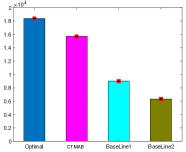
(a)

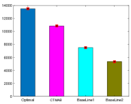
(b)

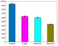
(c)

Figure 1: Comparison of cumulative reward of algorithm CTMAB with other policies for different arm means.

4.2 Lower Bound

For the multiple arm CTMAB problem we derive a lower bound on the regret of any algorithm by exploiting the fact that the algorithm has to identify the best arm with a certain probability by a certain time.

Theorem 9

Let the regret of any online algorithm for the multiple arm CTMAB problem be $g_{m}(\mu[1],\dots,\mu[K],T,\Delta)$ which can be expressed as $g_{m}(\mu[1],\dots,\mu[K],T,\Delta)=\mu[1]^{2}T^{p}_{m},$ for some $p_{m}<1$. Then $p_{m}\geq\min\{p_{1}^{m},p_{2}^{m}\},$ where

$$T^{p_{1}^{m}}=\frac{2K\log\left(\frac{c_{12}}{8}\right)}{c_{12}(\Delta/2)^{2}\mu[1]}\ \ \text{for}\ \ 0\leq p_{1}^{m}\leq 1,\quad\text{and}$$ (9)

$p_{2}^{m}=\min\left\{k\geq 0:\frac{\left(\frac{{\mathsf{c}}_{4}K}{(\Delta/2)^{2}}\log\left({\mathsf{c}}_{5}\frac{c_{12}}{8}\right)\right)^{2}}{c_{12}T^{k}}\right.$

$$\left.\quad\quad=\max\left\{\mu[1]^{2}T^{k},\mu[1]\frac{{\mathsf{c}}_{4}K}{(\Delta/2)^{2}}\log\left({\mathsf{c}}_{5}\frac{c_{12}}{8}\right)\right\}\right\},$$ (10)

where $c_{12}=\frac{\mu[1]^{2}}{\mu[2]^{2}}$ and ${\mathsf{c}}_{4},{\mathsf{c}}_{5}$ are constants.

When $\Delta$ is small, i.e., $\mu[1]\approx\mu[2]$, $p_{1}^{m}$ and $p_{2}^{m}$ satisfy $T^{p_{1}^{m}}=\Omega(\frac{K}{\mu[1]\Delta^{2}})$ and $T^{p_{2}^{m}}=\Omega(\frac{K}{\mu[1]\Delta^{2}})$. Hence the regret of any online algorithm is $g_{m}(\mu[1],\dots,\mu[K],T,\Delta)=\Omega(K\mu[1]/\Delta^{2})$ in the small $\Delta$ regime.

The main idea used to derive this lower bound is as follows. Let the regret of any algorithm $\mathcal{A}$ be $\mu[1]^{2}T^{p_{m}}$. Then consider time $T^{p_{m}+\alpha}$ for any $\alpha>0$. We show that if the probability of correctly identifying the best arm with algorithm $\mathcal{A}$ is less than $1-1/T^{\alpha}$ at time $T^{p_{m}+\alpha}$, then the regret of $\mathcal{A}$ is $>\mu[1]^{2}T^{p_{m}+\alpha}$, contradicting the assertion that the regret of $\mathcal{A}$ is $\mu[1]^{2}T^{p_{m}}$. Thus, the probability of identifying the best arm with $\mathcal{A}$ at time $T^{p_{m}+\alpha}$ must be greater than $1-1/T^{\alpha}$. This necessary condition implies a lower bound on the number of samples $N_{T^{p_{m}+\alpha}}$ to be obtained by $\mathcal{A}$ in time period $[0,T^{p_{m}+\alpha}]$ using Lemma 27. Accounting for the sampling cost resulting out of this lower bound, gives us the lower bound of Theorem 9.

Comparing the upper bound on regret for algorithm CTMAB (Theorem 8) and the lower bound (Theorem 9), we see that algorithm CTMAB achieves optimal regret up to logarithmic factors of $T$.

5 Numerical Results

In this section, we compare the performance of our algorithm against the oracle policy and a baseline policy that does not adapt to the estimates of the arm means. The baseline policy samples the optimal arm at a fixed interval of $1/aT$, where $a>0$ is a constant that determines the rate of sampling. The payoff of the baseline policy over a period $T$ is $aT(\mu[1]-\lambda a)$, and the payoff is positive and increasing for all $a\leq\frac{\mu[1]}{2\lambda}$ achieving maxima at $a=\frac{\mu[1]}{2\lambda}$.

We consider the multiple arms case, and evaluate the performance of the CTMAB algorithm with $K=5$ arms. We simulate the CTMAB algorithm on three sets of mean vectors ${\boldsymbol{\mu}}=(\mu[1],\dots,\mu[5])$, with values $(0.35,0.2,0.15,0.1,0.08),(0.3,0.2,0.15,0.1,0.08),$ and $(0.25,0.2,0.15,0.1,0.08)$, and plot the cumulative payoff for the oracle policy and the CTMAB algorithms in Fig. 1. The problem instances are chosen to have a decreasing sub-optimality gap and hence increasingly difficult to learn. As seen, the CTMAB performance is close to that of the oracle policy, and the regret degrades with reducing value of $\mu[1]$ and the sub-optimality gap. The results for the single arm case are provided in the supplementary material.

6 Conclusions

In this paper, we have a introduced a new continuous time multi-arm bandit model (CTMAB), that is well motivated from applications in crowdsourcing and inventory management systems. The CTMAB is fundamentally different than the popular DMAB, and to the best of our knowledge has not been considered before. The distinguishing feature of the CTMAB is that the oracle policy’s decision depends on the mean of the best arm, and this makes even the single arm problem non-trivial. To keep the model simple, we considered a simple sampling cost function, and derived almost tight upper and lower bounds on the optimal regret for any learning algorithm.

Appendix A Remarks on the system model

Remark 10

Unlike the DMAB setting, where algorithms like UCB or Thompson sampling can work without the knowledge of $T$, in the current setting, the CTSAB algorithm we propose, crucially uses the information about $T$ to define phases and its decisions. Developing an algorithm without the knowledge of $T$ for the CTMAB appears challenging and is part of ongoing work.

Appendix B Pseudo Code for Algorithm (CTSAB)

We use the notation $\b{1}_{x}=1$ if $x=1$ and $0$ otherwise.

Algorithm 1 Continuous Time Single Arm Bandit (CTSAB)

1:  Input $0<\epsilon<1$, $\kappa>1$, $T,\delta$

2:  %Learning Period Starts

3:  for $i=1,2,3,\ldots$ do

4:     Obtain $N_{i}=\kappa(\log T)T^{(2/3)i\epsilon}$ samples at uniform frequency in interval $[T^{(i-1)\epsilon}-\b{1}_{\{i=1\}},\ \ T^{i\epsilon}]$

5:     $N^{i}=\sum_{j\leq i}N_{j},{\hat{\mu}}_{i}=\frac{1}{N^{i}}\sum_{j=1}^{N^{i}}X_{i}$,

6:     if $\sqrt{\frac{\log(2/\delta)}{N^{i}}}<\frac{{\hat{\mu}}_{i}}{2}$ then

7:        Set $i^{\star}=i$ and Break;

8:     end if

9:  end for

10:  %Exploit Period Starts

11:  The time at which learning period ends be $\tau$

12:  if $\tau\geq T$ then

13:     Break;

14:  else

15:     for phases  $k=i^{\star}+1,i^{\star}+2,\ldots$ do

16:        Obtain $N_{k}={\hat{\mu}}_{k-1}T^{i^{\star}\epsilon}/2$ samples at equal intervals in $[\tau+(k-1)T^{i^{\star}\epsilon},\tau+kT^{i^{\star}\epsilon}]$

17:        $N^{k}=\sum_{j\leq k}N_{j},{\hat{\mu}}_{k}=\frac{1}{N^{k}}\sum_{j=1}^{N^{k}}X_{i}$,

18:        if $\tau+kT^{i^{\star}\epsilon}\geq T$ then

19:           Break;

20:        end if

21:     end for

22:  end if

Appendix C Preliminaries

Let $X_{i}$’s be independent and identically Bernoulli distributed random variables with mean $\mu$, and ${\hat{\mu}}_{N}=\frac{1}{N}\sum_{i=1}^{N}X_{i}$.

Lemma 11

(Chernoff Bound) ${\mathbb{P}}\left(|{\hat{\mu}}_{N}-\mu|>\theta\right)\leq\exp^{-2N\theta^{2}}.$

Corollary 12

Choosing $\theta=\frac{\log\left(\frac{1}{\delta}\right)}{\sqrt{N}}$, we get that $\text{err}_{N}=|{\hat{\mu}}_{N}-\mu|=O\left(\frac{\log\left(\frac{1}{\delta}\right)}{\sqrt{N}}\right)$ with probability at least $1-\delta$.

Appendix D Proof of Theorem  5

Throughout we need the definition of $p^{\star}$ (6). To prove Theorem 5, we will need the following two Lemmas.

Lemma 13

For $\delta=\frac{1}{T^{2}}$, the learning period of algorithm CTSAB ends in at most $\left(\frac{p^{\star}}{\epsilon}+1\right)$ phases, i.e., $i^{\star}\leq\left(\frac{p^{\star}}{\epsilon}+1\right)$, with probability at least $1-1/T^{2}$, where $\epsilon$ is such that $T^{\epsilon}={\mathsf{c}}$ (constant).

Note that $\frac{p^{\star}}{\epsilon}$ need not be an integer, and to be precise, we should use $\lceil\frac{p^{\star}}{\epsilon}\rceil$. For ease of exposition, however, we ignore the ceiling. Lemma 13 also shows that algorithm CTSAB does not fail with probability at least $1-1/T^{2}$. Proof: By the definition of phases, by the end of phase $\ell=\frac{p^{\star}}{\epsilon}+1$, the number of samples obtained by the algorithm is $N^{\ell}\geq(\kappa\log(T))T^{2/3(p^{\star}+\epsilon)}$, where $p^{\star}$ has been defined in (6). Moreover, from the definition of $p^{\star}$ (6), we have $\frac{1}{\mu^{4}T^{p^{\star}}}\leq\left(\mu^{2}T^{p^{\star}}\right)$. This implies that

$$\sqrt{\frac{1}{T^{2p^{\star}/3}}}\leq\mu.$$ (11)

Let $\delta=1/T^{2}$. Then

$$\sqrt{\frac{\log(2/\delta)}{N^{\ell}}} \leq\sqrt{\frac{\log(2T^{2})}{(\kappa\log(T))T^{2/3(p^{\star}+\epsilon)}}}$$

$$\leq\mu\sqrt{\frac{\log(2T^{2})}{(\kappa\log(T))T^{(2/3)\epsilon}}},$$ (12)

where the final inequality follows from (11). For any fixed $\epsilon>0$, such that $T^{\epsilon}={\mathsf{c}}$ a constant, for a large enough constant $\kappa$, we get $\mu\sqrt{\frac{\log(2T^{2})}{(\kappa\log(T))T^{(2/3)\epsilon}}}\leq\frac{\mu}{3}$. Using this fact in (12), we get

$$\sqrt{\frac{\log(2/\delta)}{N^{\ell}}}\leq\frac{\mu}{3}.$$ (13)

Recall from Corollary 12 that ${\mathbb{P}}\left(|{\hat{\mu}}_{\ell}-\mu|=\text{err}_{\ell}\geq\sqrt{\frac{\log(2/\delta)}{N^{\ell}}}\right)\leq\delta$. Thus, with probability at least $1-\delta$, we have

$${\hat{\mu}}_{\ell}\geq\mu-\text{err}_{\ell} \geq\mu-\sqrt{\frac{\log(2/\delta)}{N^{\ell}}},$$

$$\stackrel{{\scriptstyle(a)}}{{\geq}}3\sqrt{\frac{\log(2/\delta)}{N^{\ell}}}-\sqrt{\frac{\log(2/\delta)}{N^{\ell}}},$$

$$=2\sqrt{\frac{\log(2/\delta)}{N^{\ell}}}$$

at the end of phase $\ell=\frac{p^{\star}}{\epsilon}+1$, where $(a)$ follows from (13). Thus, the learning period of algorithm CTSAB is completed by the $\ell^{th}$ phase, and the algorithm CTSAB never fails with probability at least $1-\delta$, with $\delta=\frac{1}{T^{2}}$. $\Box$

From the definition of algorithm CTSAB, the total number of samples $N^{i^{\star}}$ obtained by it in the learning period satisfies

$$(\kappa\log(T))T^{(2/3)i^{\star}\epsilon} \leq N^{i^{\star}}=\sum_{i=1}^{i^{\star}}(\kappa\log(T))T^{2/3i\epsilon}$$ (14)

$$\leq(\kappa\log(T))T^{2/3(i^{\star}+1)\epsilon}.$$

since the learning phase gets over in phase $i^{\star}$ and in each phase $(\kappa\log(T))T^{(2/3)i^{\star}\epsilon}$ samples are obtained. Using this bound we get the following result.

Lemma 14

The total payoff of the CTSAB algorithm in the learning period is

$$P_{L}\geq\mu(\kappa\log(T))T^{(2/3)i^{\star}\epsilon}-(\kappa\log(T))^{2}T^{(i^{\star}+1)\epsilon/3}.$$

Proof: The total payoff of the CTSAB algorithm in the learning period by counting the payoff in each of the phase of the learning phases is

$$P_{L} =\mu N^{i^{\star}}-\sum_{i=1}^{i^{\star}}\frac{((\kappa\log(T))T^{2/3i\epsilon})^{2}}{T^{i\epsilon}-T^{(i-1)\epsilon}}$$

$$\geq\mu(\kappa\log(T))T^{(2/3)i^{\star}\epsilon}-\sum_{i=1}^{i^{\star}}\frac{((\kappa\log(T))T^{2/3i\epsilon})^{2}}{T^{i\epsilon}/2},$$

$$=\mu(\kappa\log(T))T^{(2/3)i^{\star}\epsilon}-2(\kappa\log(T))^{2}T^{(i^{\star}+1)\epsilon/3},$$ (15)

where the first inequality follows since $T^{i\epsilon}-T^{(i-1)\epsilon}\geq T^{i\epsilon}/2$, while the number of samples obtained by algorithm CTSAB in the learning period is as given by (14). $\Box$

Next simple lemma helps to show that once the learning period is complete in a particular phase, in subsequent phases the payoff obtained by CTSAB algorithm is positive.

Lemma 15

Let the number of samples obtained be $N$, and $|{\hat{\mu}}_{N}-\mu|=\text{err}_{N}$. If $\text{err}_{N}<\frac{{\hat{\mu}}_{N}}{2}$, then $\text{err}_{N}<\mu$.

Proof: By definition, $\mu={\hat{\mu}}_{N}-\text{err}_{N}$. Therefore, if $\text{err}_{N}<\frac{{\hat{\mu}}_{N}}{2}$, it implies that ${\hat{\mu}}_{N}-\text{err}_{N}>\text{err}_{N}$ which is sufficient for $\text{err}_{N}<\mu$. $\Box$

Now we complete the Proof of Theorem  5. From Corollary 12, at the end of phase $i$, $\text{err}_{i}\leq\sqrt{\frac{\log(2/\delta)}{N^{i}}}$ with probability at least $1-\delta$, where $N^{i}$ is total number of samples obtained until the end of phase $i$. Thus, the condition that ends the training period in phase $i^{\star}$, $\sqrt{\frac{\log(2/\delta)}{N^{i^{\star}}}}<\frac{{\hat{\mu}}_{i^{\star}}}{2}$ ensures that $\text{err}_{i^{\star}}<\frac{{\hat{\mu}}_{i^{\star}}}{2}$ with probability at least $1-\delta$, which implies that $\text{err}_{i^{\star}}<\mu$ (Lemma 15). For phase $i>i^{\star}$, obtaining ${\hat{\mu}}_{i}T^{i^{\star}\epsilon}/2$ samples in each phase, the payoff obtained by algorithm CTSAB in phase $i$ is

$$P_{i} =\mu\frac{{\hat{\mu}}_{i}T^{i^{\star}\epsilon}}{2}-\frac{(\frac{{\hat{\mu}}_{i}T^{i^{\star}\epsilon}}{2})^{2}}{T^{i^{\star}\epsilon}},$$

$$=\mu\frac{(\mu\pm\text{err}_{i})T^{i^{\star}\epsilon}}{2}-\frac{(\frac{(\mu\pm\text{err}_{i})T^{i^{\star}\epsilon}}{2})^{2}}{T^{i^{\star}\epsilon}},$$

$$\geq\frac{\mu^{2}T^{i^{\star}\epsilon}}{4}-\text{err}_{i}^{2}\frac{T^{i^{\star}\epsilon}}{4}.$$ (16)

Since at the end of learning period phase $i^{\star}$, $\text{err}_{i^{\star}}<\mu$, hence, we have that $P_{i}>0$ for $i>i^{\star}$.

Let the bad event in phase $j$ be defined as $B_{j}=\{\text{err}_{j}>\frac{c}{\sqrt{N^{j}}}\}$, where $N^{j}$ is the sum of the number of samples obtained until the end of phase $j$. For further analysis of the payoff of algorithm CTSAB in the exploit period, we want to bound the probability that a bad event happens during any phase (both in learning and exploit period).

Lemma 16

The probability that a bad event happens in any phase of learning or exploit period of algorithm CTSAB is $\leq 1-\frac{T}{T^{\epsilon}}\delta$ for $c=\sqrt{\log(2/\delta)/2}$.

Proof: From Corollary 12, we know that ${\mathbb{P}}(B_{j})\leq\delta$, if $c=\sqrt{\log(2/\delta)/2}$. Thus, the probability that in any phase (both in learning period and beyond), a bad event happens ${\mathbb{P}}(\cup_{j}B_{j})\leq\frac{T}{T^{\epsilon}}{\mathbb{P}}(B_{j})\leq\frac{T}{T^{\epsilon}}\delta$, since there are at most $\frac{T}{T^{\epsilon}}$ phases in all (counting both the learning period and the exploit period). $\Box$

From here on, we will assume that during no phase a bad event happens, and account for its probability $1-\frac{T}{T^{\epsilon}}\delta$ appropriately.

Recall that with the exploit period of algorithm CTSAB, assuming ${\hat{\mu}}_{i}$ to the true value of $\mu$, the number of samples to be obtained in phase $i+1,i\geq i^{\star}$, is given by $\frac{{\hat{\mu}}_{i}T^{i^{\star}\epsilon}}{2}$. Thus, the total number of samples obtained by the end of phase $i>i^{\star}$ (for all $i>i^{\star}$) is given by

$$N^{i} \geq(\kappa\log T)T^{(2/3)i^{\star}\epsilon}+\sum_{j=i^{\star}+1}^{i}{\hat{\mu}}_{j}\frac{T^{i^{\star}\epsilon}}{2},$$

$$=(\kappa\log T)T^{(2/3)i^{\star}\epsilon}+\sum_{j=i^{\star}+1}^{i}(\mu\pm\text{err}_{j})\frac{T^{i^{\star}\epsilon}}{2},$$

$$\stackrel{{\scriptstyle(a)}}{{\geq}}(\kappa\log T)T^{(2/3)i^{\star}\epsilon}+\sum_{j=i^{\star}+1}^{i}\left(\mu\pm\frac{c}{\sqrt{N_{j-1}}}\right)\frac{T^{i^{\star}\epsilon}}{2},$$

$$\geq\mu T^{i^{\star}\epsilon}\frac{i-i^{\star}}{2}-o(T^{i^{\star}\epsilon}),$$ (17)

where $(a)$ follows from Lemma 16 $\forall j\leq i$. Therefore using (17), from Lemma 16, we get $\text{err}_{i}\leq\sqrt{\frac{2\ln(2/\delta)}{2\mu(i-i^{\star})T^{i^{\star}\epsilon}}}$ with probability at least $1-\frac{T}{T^{\epsilon}}\delta$ for all phases $i\geq i^{\star}+1$. Thus, with probability at least $1-\frac{T}{T^{\epsilon}}\delta$, for phase $i\geq i^{\star}+1$, following (16), the payoff obtained in phase $i$

$$P_{i} \geq\frac{\mu^{2}T^{i^{\star}\epsilon}}{4}-\frac{2\ln(2/\delta)}{2\mu(i-i^{\star})T^{i^{\star}\epsilon}}\frac{T^{i^{\star}\epsilon}}{4},$$

$$\geq\frac{\mu^{2}T^{i^{\star}\epsilon}}{4}-\frac{\ln(2/\delta)}{4\mu(i-i^{\star})}.$$ (18)

Algorithm CTSAB fails with probability at most $\delta$, and the probability that any bad event happens is at most $\frac{T}{T^{\epsilon}}\delta$. Thus, with probability $1-\delta-\frac{T}{T^{\epsilon}}\delta$ neither the Algorithm CTSAB fails nor any of the bad events happen. Thus, combining (15) and (18) the total payoff for the CTSAB algorithm is

$$P =P_{L}+\sum_{i=i^{\star}+1}^{\frac{T-T^{i^{\star}\epsilon}}{T^{i^{\star}\epsilon}}}P_{i},$$

$$\geq\mu(\kappa\log(T))T^{(2/3)i^{\star}\epsilon}-2(\kappa\log(T))^{2}T^{(i^{\star}+1)\epsilon/3}+\sum_{i=i^{\star}+1}^{\frac{T-T^{i^{\star}\epsilon}}{T^{i^{\star}\epsilon}}}\frac{\mu^{2}T^{i^{\star}\epsilon}}{4}-\sum_{i=i^{\star}+1}^{\frac{T-T^{i^{\star}\epsilon}}{T^{i^{\star}\epsilon}}}\frac{\ln(2/\delta)}{4\mu(i-i^{\star})},$$

$$\geq\mu(\kappa\log(T))T^{(2/3)i^{\star}\epsilon}-2(\kappa\log(T))^{2}T^{(i^{\star}+1)\epsilon/3}+\frac{\mu^{2}(T-T^{(i^{\star}+1)\epsilon})}{4}-\frac{\ln(2/\delta)}{4\mu}\ln\left(\frac{T}{T^{i^{\star}\epsilon}}\right),$$ (19)

with probability at least $1-\frac{T}{T^{\epsilon}}\delta-\delta$, where in the final inequality, the third term follows since the total length of the learning period is at most $T^{(i^{\star}+1)\epsilon}$, while in the final term we have used a simple upper bound $\sum_{i=i^{\star}+1}^{\frac{T-T^{i^{\star}\epsilon}}{T^{i^{\star}\epsilon}}}\frac{1}{(i-i^{\star})}\leq\ln\left(\frac{T}{T^{i^{\star}\epsilon}}\right)$. Recall that the payoff of the oracle policy is $\frac{\mu^{2}T}{4}$. Thus the regret of CTSAB algorithm is at most

$$R \leq 2(\kappa\log(T))^{2}T^{(i^{\star}+1)\epsilon/3}+\frac{\mu^{2}T^{(i^{\star}+1)\epsilon}}{4}+\frac{\ln(2/\delta)}{4\mu}\ln\left(\frac{T}{T^{i^{\star}\epsilon}}\right),$$

$$\stackrel{{\scriptstyle(a)}}{{=}}O((\log(T))^{2}T^{p^{\star}/3}T^{4\epsilon/3})+O((\mu^{2})T^{p^{\star}+\epsilon})O(\mu^{2}T^{p^{\star}+\epsilon/3}\ln(2/\delta)\ln(T)),$$

$$\stackrel{{\scriptstyle(b)}}{{=}}O\left((\log(T))^{2}\frac{1}{\mu}T^{4\epsilon/3}\right)+O(\mu^{2}T^{p^{\star}+\epsilon^{\prime}}\ln(2/\delta)\ln(T)),$$

$$\stackrel{{\scriptstyle(c)}}{{=}}O((\log(T))^{2}\mu^{2}T^{p^{\star}}T^{4\epsilon/3})+O(\mu^{2}T^{p^{\star}+\epsilon^{\prime}}\ln(2/\delta)\ln(T)),$$ (20)

with probability $1-\frac{T}{T^{\epsilon}}\delta-\delta$, where in $(a)$ the first term follows since $i^{\star}\epsilon\leq p^{\star}+\epsilon$ (Lemma 13), and the third term using the definition of $p^{\star}$ (6), while to get $(b)$ we use (6) and $\epsilon^{\prime}=4/3\epsilon$, $(c)$ follows since $\left(\frac{1}{\mu}\right)=O\left(\mu^{2}T^{p^{\star}}\right)$ from (6).

Remark 17

Given that the arm reward distribution is Bernoulli, $\text{err}_{i}$ is bounded at the end of each phase $i$ with the CTSAB algorithm. Thus, following (25), the regret of CTSAB algorithm is at most $O(T)$.

With $\delta=1/T^{2}$, and since the maximum regret can be $O(T)$ (Remark 17), from (20) we get that the expected regret of the CTSAB algorithm is

$$\mathcal{R}={\mathbb{E}}\{R\} =O(\mu^{2}T^{p^{\star}+\epsilon^{\prime}}\ln(2/\delta)\ln(T))(1-\frac{T}{T^{\epsilon}}\delta-\delta)$$

$$+O(T)\left(\frac{T}{T^{\epsilon}}\delta+\delta\right),$$

$$=O(\mu^{2}T^{p^{\star}+\epsilon^{\prime}}\ln(2T^{2})\ln(T))(1-\frac{T}{T^{\epsilon}}\frac{1}{T^{2}}-\frac{1}{T^{2}})$$

$$+O(T)\left(\frac{1}{T^{1+\epsilon}}+\frac{1}{T^{2}}\right),$$

$$=O(\mu^{2}T^{p^{\star}+\epsilon^{\prime}}\ln(2T^{2})\ln(2T))(1-\frac{1}{T^{1+\epsilon}}-\frac{1}{T^{2}})$$

$$+O(T)\left(\frac{1}{T^{1+\epsilon}}+\frac{1}{T^{2}}\right).$$

This completes the proof of Theorem 5.

Appendix E Preliminaries to prove Theorem 7

To lower bound the regret of any algorithm for the single arm CTMAB, we will need the following preliminaries.

Prediction Problem : Consider two Bernoulli distributions $\mathcal{P}$ and $\mathcal{Q}$ with means $x$ and $x+\beta$, respectively, where $x>0,\beta>0$. A coin is tossed repeatedly with probability of heads distributed according to either $\mathcal{P}$ or $\mathcal{Q}$, where repeated tosses are independent. From the observed samples, the problem is to predict the correct distribution $\mathcal{P}$ or $\mathcal{Q}$ such that the success probability of the prediction is at least $1-\gamma$.

Lemma 18

Let $n$ be fixed. Consider any algorithm $\mathcal{A}_{n}$ that obtains $n$ samples and solves the prediction problem with success probability at least $1-\gamma$. Then $n>\left(\frac{\ln 2}{8\beta^{2}}\log\left(\frac{1}{4\gamma}\right)\right)$ for $\beta<1/4$.

Proof: Let the product distribution over $n$ samples derived from $\mathcal{P}$ and $\mathcal{Q}$ be $\mathcal{P}^{n}$ and $\mathcal{Q}^{n}$. Let $E$ be the event that the algorithm $\mathcal{A}_{n}$ outputs $\mathcal{P}$ as the correct distribution, and $E^{c}$ be its complement. Then from Theorem 14.2 Lattimore and Szepesvári [2020], we have that

$${\mathbb{P}}_{\mathcal{P}}(E^{c})+{\mathbb{P}}_{\mathcal{Q}}(E)\geq\frac{1}{2}\exp\left(-D(\mathcal{P}^{n}||\mathcal{Q}^{n})\right),$$ (21)

where $D(\mathcal{P}^{n}||\mathcal{Q}^{n})$ is the Kullback-Liebler distance between $\mathcal{P}^{n}$ and $\mathcal{Q}^{n}$. Since the probability of success for $\mathcal{A}_{n}$ is $\geq 1-\gamma$, we have that both ${\mathbb{P}}_{\mathcal{P}}(E^{c})<\gamma$ and ${\mathbb{P}}_{\mathcal{Q}}(E)<\gamma$. Thus, from (21), we get

$$2\gamma>\frac{1}{2}\exp\left(-D(\mathcal{P}^{n}||\mathcal{Q}^{n})\right).$$ (22)

Moreover, we have that $D(\mathcal{P}^{n}||\mathcal{Q}^{n})=nD(\mathcal{P}||\mathcal{Q})$, and $D(\mathcal{P}||\mathcal{Q})\leq\frac{8\beta^{2}}{\ln 2}$ for $\beta\leq 1/4$ for $\mathcal{P}$ and $\mathcal{Q}$ being Bernoulli with means $x$ and $x+\beta$.

Therefore, we get that

$$4\gamma>\exp\left(-\frac{n8\beta^{2}}{\ln 2}\right),$$ (23)

which implies the result. $\Box$ In addition to Lemma 18, we need the following Lemma that is specific to the considered problem. Let an algorithm $\mathcal{A}$ obtain $N_{t}$ samples in time $[0,t]$. Recall that ${\hat{\mu}}_{t}=\frac{1}{N_{t}}\sum_{i=1}^{N_{t}}X_{i}$ is the empirical average of the reward obtained by $\mathcal{A}$ using the $N_{t}$ samples, where ${\mathbb{E}}\{X_{i}\}=\mu,\ \forall\ i$ and $\text{err}_{t}=|{\hat{\mu}}_{t}-\mu|$ is the error in estimating $\mu$ by $\mathcal{A}$ at time $t$.

Lemma 19

For an online algorithm $\mathcal{A}$ (satisfying Assumption 6) the maximum payoff possible in interval $[0,t]$ is at most $\frac{\mu^{2}t}{4}-\text{err}_{t}^{2}\frac{t}{4}$.

Proof: Recall that we are considering algorithms that only use unbiased estimates of $\mu$ to make decisions as described in Remark 6. For any algorithm $\mathcal{A}$, let the (sample mean) estimate of $\mu$ at time $t$ be ${\hat{\mu}}_{t}$ where $\text{err}_{t}=|{\hat{\mu}}_{t}-\mu|$. We want to upper bound the expected payoff of $\mathcal{A}$ in $[0,t]$. Towards that end, we bound the expected payoff if $\mathcal{A}$ knew ${\hat{\mu}}_{t}$ at time $0$ itself, which can only improve the lower bound.

Note that with Bernoulli distribution, the empirical estimate ${\hat{\mu}}_{t}$ is a sufficient and complete statistic Kay [1993] for $\mu$, and the minimum variance unbiased estimator (MVUE) for $\mu$.

Knowing ${\hat{\mu}}_{t}$ at time $0$, let $N({\hat{\mu}}_{t})$ be the number of samples obtained (at equal intervals since it minimizes the sampling cost) by algorithm $\mathcal{A}$ in time $[0,t]$. Then maximizing the expected payoff of $\mathcal{A}$ in interval $[0,t]$ is equivalent to minimizing the expected regret (3) of $\mathcal{A}$ in $[0,t]$, given by

$$\mathcal{R}([0,t]) =\min_{N({\hat{\mu}}_{t})}{\mathbb{E}}\left\{\frac{\mu^{2}t}{4}-\mu N({\hat{\mu}}_{t})+\frac{1}{t}N({\hat{\mu}}_{t})^{2}\right\},$$

$$=\min_{N({\hat{\mu}}_{t})}{\mathbb{E}}\left\{\left(\sqrt{\frac{t}{4}}\mu-\sqrt{\frac{1}{t}}N({\hat{\mu}}_{t})\right)^{2}\right\},$$

$$=\min_{N({\hat{\mu}}_{t})}{\mathbb{E}}\left\{\frac{t}{4}\left(\mu-\frac{2}{t}N({\hat{\mu}}_{t})\right)^{2}\right\}.$$ (24)

Since ${\hat{\mu}}_{t}$ is MVUE for $\mu$, the number of samples $N^{\star}({\hat{\mu}}_{t})$ that $\mathcal{A}$ obtains to minimize regret (24) (and maximize the expected payoff) knowing ${\hat{\mu}}_{t}$ at time $0$ in $[0,t]$ is ${\hat{\mu}}_{t}t/2$.

Therefore, the upper bound on the payoff of $\mathcal{A}$ in time $[0,t]$ is

$$P([0,t]) \leq\mu N^{\star}({\hat{\mu}}_{t})-(N^{\star}({\hat{\mu}}_{t}))^{2}/t,$$

$$=\frac{\mu^{2}t}{4}-\text{err}_{t}^{2}\frac{t}{4},$$ (25)

where $\text{err}_{t}=|{\hat{\mu}}_{t}-\mu|.$

$\Box$

Appendix F Basic idea for proving Theorem 7

Using Lemma 18, we next derive a lower bound on the regret of any algorithm for the single arm CTMAB problem. The basic idea used to derive the lower bound is that if suppose the regret of any algorithm $\mathcal{A}$ is $\mu^{2}T^{p}$, then we show that with $\mathcal{A}$ it must be that at time $T^{p+\alpha}$ for some $\alpha>0$, the probability that $\text{err}_{T^{p+\alpha}}>\mu/T^{\alpha/4}$ (error in estimating $\mu$ at time $T^{p+\alpha}$ is greater than $\mu/T^{\alpha/4}$) is at most $1/T^{\alpha/2}$. This condition is necessary, since otherwise Lemma 19 implies that the regret of $\mathcal{A}$ is $>\mu^{2}T^{p}$ contradicting the regret bound of $\mu^{2}T^{p}$. The necessary condition ${\mathbb{P}}(\text{err}_{T^{p+\alpha}}>\mu/T^{\alpha/4})<1/T^{\alpha/2}$ implies a lower bound on the number of samples to be obtained by $\mathcal{A}$ in interval $[0,T^{p+\alpha}]$ from Lemma 18. Accounting for the sampling cost resulting out of this lower bound on the number of samples gives us the required lower bound on the regret.

Appendix G Proof of Theorem 7

Proof: Consider any online algorithm $\mathcal{A}$ for the single arm CTMAB for which Assumption 6 holds. Let the regret of $\mathcal{A}$ be $g(\mu,T)$ which can be expressed as $g(\mu,T)=\mu^{2}T^{p}$ for some $p<1$, since recall that the oracle payoff in time interval $[0,T]$ is $\mu^{2}T/4$.

We divide the total time horizon $T$ into two intervals, first $[0,T^{p+\alpha}]$, and second $[T^{p+\alpha},T]$.

Let $\mathcal{A}$ know that the true mean is either $\mu$ or $\mu+\frac{2\mu}{T^{\alpha/4}}$ for some $\alpha>0$ that we will specify later. This assumption can only reduce the regret of any algorithm. Let the true mean be $\mu_{\text{true}}\in\{\mu,\mu+\frac{2\mu}{T^{\alpha/4}}\}$.

Let the number of samples obtained by $\mathcal{A}$ till time $T^{p+\alpha}$ be $N_{\mathcal{A}}(T^{p+\alpha})$ and $N_{\min}=\frac{c_{1}T^{\alpha/2}}{\mu^{2}}\log(c_{2}T^{\alpha/2})$. Assume that $N_{\mathcal{A}}(T^{p+\alpha})<N_{\min}$. From Lemma 18, if the number of samples $N_{\mathcal{A}}(T^{p+\alpha})$ is less than $N_{\min}$, then ${\mathbb{P}}(\text{err}_{N_{\mathcal{A}}(T^{p+\alpha})}=|{\hat{\mu}}_{N_{T^{p+\alpha}}}-\mu_{\text{true}}|>\frac{\mu}{T^{\alpha/4}})>\frac{1}{T^{\alpha/2}}$. Note that even though $N_{\mathcal{A}}(T^{p+\alpha})$ is a random variable (depending on the realizations seen by $\mathcal{A}$ till time $T^{p+\alpha}$), we are applying Lemma 18 since it is true for any algorithm that obtains a given number of samples, in particular $N_{\mathcal{A}}(T^{p+\alpha})$.

Without loss of generality, let $\mu_{\text{true}}=\mu$. Moreover, define ${\mathbb{P}}_{b}(t)={\mathbb{P}}(\text{err}_{N_{T^{p+\alpha}}}>\frac{\mu}{T^{\alpha/4}})$, and ${\mathbb{P}}_{g}(t)=1-{\mathbb{P}}_{b}(t)$.

Then the payoff of algorithm $\mathcal{A}$ over the two intervals $[0,T^{p+\alpha}]$, and $[T^{p+\alpha},T]$ can be written as

$$P_{\mathcal{A}} =P_{\mathcal{A}}([0,T^{p+\alpha})]+P_{\mathcal{A}}([T^{p+\alpha},T]),$$

$$\stackrel{{\scriptstyle(a)}}{{\leq}}{\mathbb{P}}_{g}(T^{p+\alpha})\frac{\mu^{2}(T^{p+\alpha})}{4}+{\mathbb{P}}_{b}(T^{p+\alpha})\cdot\left(\mu^{2}\frac{T^{p+\alpha}}{4}-\frac{\mu^{2}}{T^{p+\alpha/2}}\frac{T^{p+\alpha}}{4}\right)+\frac{\mu^{2}(T-T^{p+\alpha})}{4},$$

$$\stackrel{{\scriptstyle(b)}}{{=}}-\mu^{2}(T^{p+\alpha/2})\frac{{\mathbb{P}}_{b}(T^{p+\alpha})}{4}+\mu^{2}\frac{T}{4}.$$ (26)

where the first two terms of $(a)$ follow as detailed next, case i) when $\text{err}_{N_{\mathcal{A}}(T^{p+\alpha})}\geq\frac{\mu}{T^{\alpha/4}}$ using (25), while in case ii) when $\text{err}_{N_{\mathcal{A}}(T^{p+\alpha})}<\frac{\mu}{T^{\alpha/4}}$, making $\text{err}_{N_{\mathcal{A}}(T^{p+\alpha})}=0$ and getting the oracle payoff $\frac{\mu^{2}(T^{p+\alpha})}{4}$, while for the third term we let $P_{\mathcal{A}}([T^{p+\alpha},T])$ to be the oracle’s payoff for interval $[T^{p+\alpha},T]$. As discussed earlier, given that $N_{\mathcal{A}}(T^{p+\alpha})<N_{\min}$, ${\mathbb{P}}_{b}(T^{p+\alpha})>\frac{1}{T^{\alpha/2}}$. Using this fact, $(b)$ implies that the regret ($\mu^{2}T/4-P_{\mathcal{A}}$) of $\mathcal{A}$ is larger than $\mu^{2}T^{p}$ giving us a contradiction. Therefore, for $\mathcal{A}$ to have regret $\mu^{2}T^{p}$, it is necessary that $N_{\mathcal{A}}(T^{p+\alpha})\geq N_{\min}$.

As a function of $N_{\mathcal{A}}(T^{p+\alpha})$, we can write the payoff of $\mathcal{A}$ as

$$P_{\mathcal{A}} =P_{\mathcal{A}}([0,T^{p+\alpha})]+P_{\mathcal{A}}([T^{p+\alpha},T]),$$

$$\stackrel{{\scriptstyle(a)}}{{\leq}}\mu N_{\mathcal{A}}(T^{p+\alpha})-\frac{N^{2}_{\mathcal{A}}(T^{p+\alpha})}{T^{p+\alpha}}+\frac{\mu^{2}(T-T^{p+\alpha})}{4},$$ (27)

where in $(a)$ for the first interval the bound follows since the sampling cost is smallest if $N_{\mathcal{A}}(T^{p+\alpha})$ samples are obtained at uniform intervals in $[0,T^{p+\alpha}]$, while for the second term $P_{\mathcal{A}}([T^{p+\alpha},T])$ assuming that the algorithm $\mathcal{A}$ knows the true value of $\mu$ at time $T^{p+\alpha}$, and obtains the payoff equal to that of the oracle policy for interval $[T^{p+\alpha},T]$.

Remark 20

From (27), the payoff in the first interval $\mu x-\frac{x^{2}}{T^{p+\alpha}}$ (where $x$ is the number of samples obtained in time $[0,T^{p+\alpha}])$ is a concave and unimodal function of $x$ with optimal $x^{\star}=\frac{\mu T^{p+\alpha}}{2}$.

Thus, we consider two cases : i) $x^{\star}\geq N_{\min}$ and ii) $x^{\star}<N_{\min}$.

Case i) When $x^{\star}\geq N_{\min}$, using expressions for $x^{\star}$ and $N_{\min}$, we get that

$$\frac{\mu T^{p+\alpha}}{2}\geq c_{1}T^{\alpha/2}\log(c_{2}T^{\alpha/2})/\mu^{2},$$

implying

$$T^{p+\alpha}\geq\frac{2c_{1}T^{\alpha/2}}{\mu^{3}}\log(c_{2}T^{\alpha/2})\quad\forall\ \alpha>0.$$ (28)

Choosing $T^{\alpha/2}=c>1$ (a constant), i.e. $\alpha=\frac{2\log c}{\log(T)}$, gives

$$T^{p}\geq\frac{2c_{1}}{c\mu^{3}}\log(c_{2})+\frac{2c_{1}}{c\mu^{3}}2\log(c)\frac{\log(T)}{\log(T)}.$$

Thus,

$$p\geq\min\left\{k\geq 0:T^{k}\geq\frac{{\mathsf{c}}_{1}}{\mu^{3}}\right\},$$ (29)

where ${\mathsf{c}}_{1}$ is a constant. For case ii) we proceed as follows. We have already argued that $N_{\mathcal{A}}(T^{p+\alpha})\geq N_{\min}$. Thus, following Remark 20, with $x^{\star}<N_{\min}$, it is clear that the RHS of (27) is a decreasing function of $N_{T^{p+\alpha}}\geq N_{\min}$ for fixed $\mu$ and $T$. Thus, choosing $N_{\mathcal{A}}(T^{p+\alpha})=N_{\min}$ (the minimum possible), from (27), we obtain the largest expected payoff of algorithm $\mathcal{A}$ for the first interval, and the overall expected payoff over the two intervals is

$$P_{\mathcal{A}} \leq\mu N_{\min}-\frac{1}{T^{p+\alpha}}N_{\min}^{2}+\frac{\mu^{2}(T-T^{p+\alpha})}{4}.$$

Thus, for the regret of algorithm $\mathcal{A}$ to be $\mu^{2}T^{p}$, we need

$$\frac{N_{\min}^{2}}{T^{p+\alpha}}\leq\mu^{2}T^{p}+\mu N_{\min}.$$

Substituting for the value of $N_{\min}$, recalling that $T^{\alpha/2}=c>1$ and using the fact that $a+b\leq\max\{2a,2b\}$, we get

$$p\geq\min\left\{k\geq 0:\frac{1}{T^{k}}\left(\frac{{\mathsf{c}}_{2}}{\mu^{2}}\right)^{2}=2\max\left\{\mu^{2}T^{k},\frac{{\mathsf{c}}_{2}}{\mu}\right\}\right\},$$ (30)

where ${\mathsf{c}}_{2}$ is a constant.

$\Box$ Generalizing the lower bound derived in Theorem 7 to allow for biased estimators appears to be technically challenging since biased estimators with minimum variance are difficult to find, as well as if found, tend to depend on the parameter to be estimated, making them unrealizable Kay [1993].

Appendix H Extensions to general sampling cost functions

Remark 21

Extension of Theorem 5 and Theorem 7 (with the same algorithm CTSAB where the sampling frequency is chosen so as to optimize (2)) to general convex functions $f$ for the sampling cost, other than $f(x)=1/x$ is readily possible. Specifically, Prop. 1 remains unchanged as long as $f$ is convex, while the optimal payoff in Prop. 2 will depend on the exact function $f$. Moreover, other arguments made to derive Theorem 7 and Theorem 5 can also be extended for general $f$, however, deriving exact expressions similar to the lower bound Theorem 7 and upper bound Theorem 5 requires extra work, that is beyond the scope of this paper.

Appendix I Pseudo Code for Algorithm (CTMAB)

Algorithm 2 Continuous Time Multi-Arm Bandit (CTMAB)

1:  Input $0<\epsilon<1$, $\kappa>1$, $T,\delta$

2:  $\b{1}_{x}=1$ if $x=1$ and $0$ otherwise

3:  %Estimation Period Starts

4:  for phases $i=1,2,3,\ldots$ do

5:     Obtain $N_{i}[j]=\kappa\log(T)T^{(2/3)i\epsilon}$ samples at uniform frequency for each arm $j,j=1,\dots,K,$ simultaneously in interval $[T^{(i-1)\epsilon}-\b{1}_{i=1},\ \ T^{i\epsilon}]$

6:     After every sampling time $t$ in each phase, $N^{t}[j]$ is the number of samples obtained for arm $j$ till time $t$, and empirical mean for arm $j$, ${\hat{\mu}}_{t}[j]=\frac{1}{N^{t}[j]}\sum_{k=1}^{N^{t}[j]}X_{k}$,

7:     if $\sqrt{\frac{\log(2/\delta)}{N^{t}[k]}}<\frac{{\hat{\mu}}_{t}[k]}{2}$  for any arm  $k$  then

8:        Let $a_{t}$ be the index of the arm with the largest estimated mean i.e.

9:        $a_{t}=\arg\max_{j=1,\dots,K}{\hat{\mu}}_{t}[j]$,

10:        Define ${\hat{\mu}}[1]={\hat{\mu}}_{t}[a_{t}]$, set $i^{\star}=i$ (phase index) and Break;

11:     end if

12:  end for

13:  Let the time at which the estimation period end be $t_{\text{Es}}$

14:  if $t_{\text{Es}}\geq T$ then

15:     Break;

16:  else

17:     %Begin identification period

18:     Execute Best Arm Identification using the LUCB1 algorithm Kalyanakrishnan et al. [2012] with input ($K$ arms, required probability of success $1-\delta=1-1/T^{2}$ ), where arms to be sampled by LUCB1 are sampled at frequency one sample per $1/{\hat{\mu}}[1]$ time

19:     Let $k^{\star}$ be the arm identified by the LUCB1 as the best arm

20:     Let Algorithm LUCB1 terminate at time $t_{\text{Es}}+t_{\text{Id}}$

21:     if $t_{\text{Es}}+t_{\text{Id}}\geq T$ then

22:        Break;

23:     else

24:        After the end of identification period at time $t_{\text{Es}}+t_{\text{Id}}$, consider only the $k^{\star}$-th arm

25:        %Execute Exploit Period of Algorithm 1

26:        Let $N^{[1]}$ be the total number of samples obtained for the $k^{\star}$-th arm in the estimation and identification period

27:        ${\hat{\mu}}_{1}=\frac{1}{N^{[1]}}\sum_{i=1}^{N^{[1]}}X_{k^{\star}}(i)$ empirical average of the $k^{\star}$-th arm

28:        Divide total remaining time interval $[t_{\text{Es}}+t_{\text{Id}},T]$ into $(T-t_{\text{Es}}-t_{\text{Id}})/T^{\nu_{m}}$ intervals (called phase) of width $T^{\nu_{m}}$ each, for some $\nu_{m}>0$

29:        for $r=1,2,\ldots$ do

30:           Obtain $N_{r}={\hat{\mu}}_{r}T^{\nu_{m}}/2$ samples from the $k^{\star}$-th arm at equal intervals in $[t_{\text{Es}}+t_{\text{Id}}+rT^{\nu_{m}},t_{\text{Es}}+t_{\text{Id}}+(r+1)T^{\nu_{m}}]$

31:           $N^{r}=N^{[1]}+\sum_{j\leq r}N_{j},{\hat{\mu}}_{r}=\frac{1}{N^{r}}\sum_{j=1}^{N^{r}}X_{i}$, %update the sample average

32:           if $t_{\text{Es}}+t_{\text{Id}}+(r+1)T^{\nu_{m}}\geq T$ then

33:              Break;

34:           end if

35:        end for

36:     end if

37:  end if

Appendix J

Lemma 22

With probability at least $1-3\delta$, the estimation period of the algorithm CTMAB ends by time $O(T^{p^{\star}})$, (where $p^{\star}$ is as defined in (6) with $\mu=\mu[1]$) and the empirical estimate ${\hat{\mu}}_{t}[a_{t}]$ of the chosen arm $a_{t}$ satisfies $\frac{2}{3}\mu[1]\leq{\hat{\mu}}_{t}[a_{t}]\leq 2\mu[1]$.

Proof: As defined before, let the true best arm be arm $1$. First, we argue about the estimation error, and then upper bound the time to end the estimation period.

Consider the earliest time $t$ at which $\sqrt{\frac{\log(2/\delta)}{N^{t}[k]}}<\frac{{\hat{\mu}}_{t}[k]}{2}$ is true for some arm $k$, i.e., the estimation period ends at time $t$. Recall that $a_{t}$ is defined as the index of the arm with the largest empirical mean at any sampling time $t$. We claim that either $a_{t}=k$ or $\sqrt{\frac{\log(2/\delta)}{N^{t}[a_{t}]}}<\frac{{\hat{\mu}}_{t}[a_{t}]}{2}$ is also true. In case $a_{t}\neq k$, note that by definition $\frac{{\hat{\mu}}_{t}[k]}{2}\leq\frac{{\hat{\mu}}_{t}[a_{t}]}{2}$, and hence $\sqrt{\frac{\log(2/\delta)}{N^{t}[a_{t}]}}<\frac{{\hat{\mu}}_{t}[a_{t}]}{2}$ also, since the number of samples obtained for each arm is the same, i.e. $N^{t}[k_{1}]=N^{t}[k_{2}]$, for any $k_{1}\neq k_{2}$.

Thus, we restrict our attention to arm $a_{t}$ alone for estimating the error $|{\hat{\mu}}_{t}[a_{t}]-\mu[1]|$.

Case 1: $a_{t}=1$ when the estimation period terminates. Thus, $\sqrt{\frac{\log(2/\delta)}{N^{t}[1]}}<\frac{{\hat{\mu}}_{t}[1]}{2}$. Using Corollary 12, we have that at any time, for arm $1$ with probability at least $1-\delta$, $|{\hat{\mu}}[1]-\mu[1]|\leq\sqrt{\frac{\log(1/\delta)}{N^{t}[1]}}$, which together with $\sqrt{\frac{\log(2/\delta)}{N^{t}[1]}}<\frac{{\hat{\mu}}_{t}[1]}{2}$ shows that $|{\hat{\mu}}_{t}[1]-\mu[1]|\leq{\hat{\mu}}[1]/2$ implying $\frac{2}{3}\mu[1]\leq{\hat{\mu}}_{t}[a_{t}]\leq 2\mu[1]$.

Case 2: $a_{t}\neq 1$ when the estimation period terminates. Let $a_{t}=k>1$, and $\sqrt{\frac{\log(2/\delta)}{N^{t}[k]}}<\frac{{\hat{\mu}}_{t}[k]}{2}$. Using Corollary 12, we have that at any time, for arm $1$ with probability at least $1-\delta$, ${\hat{\mu}}[1]+\sqrt{\frac{\log(1/\delta)}{N^{t}[1]}}\geq\mu[1]$. Since $a_{t}=k>1$, it must be that ${\hat{\mu}}[k]+\sqrt{\frac{\log(1/\delta)}{N^{t}[k]}}>\mu[1]$ with probability at least $1-\delta$, since with probability at least $1-\delta$, ${\hat{\mu}}[1]+\sqrt{\frac{\log(1/\delta)}{N^{t}[1]}}\geq\mu[1]$. Thus, for arm $k$, when $\sqrt{\frac{\log(2/\delta)}{N^{t}[k]}}<\frac{{\hat{\mu}}_{t}[k]}{2}$, it implies that ${\hat{\mu}}[k]+\frac{{\hat{\mu}}_{t}[k]}{2}>\mu[1]$ which means that ${\hat{\mu}}_{t}[k]\geq\frac{2}{3}\mu[1]$. As in Case 1, $\sqrt{\frac{\log(2/\delta)}{N^{t}[k]}}<\frac{{\hat{\mu}}_{t}[k]}{2}$ implies that ${\hat{\mu}}_{t}[k]\leq 2\mu[k]$ with probability at least $1-\delta$. Since arm $1$ is the true best arm $\mu[k]\leq\mu[1]$, hence we can conclude that ${\hat{\mu}}_{t}[k]\leq 2\mu[1]$.

Time for the estimation period to terminate. From Lemma 13, we know that with high probability (at least $1-\delta$) by time $T^{p^{\star}}$ ($p^{\star}$ defined in (6) with $\mu=\mu[1]$), $\sqrt{\frac{\log(2/\delta)}{N^{t}[1]}}<\frac{{\hat{\mu}}_{t}[1]}{2}$ for the true best arm, arm $1$. Since all arms are sampled simultaneously at equal frequency, thus, the estimation period ends by time at most $T^{p^{\star}}$ with probability $1-\delta$.

Taking the union over all the bad events (at most three of them each with probability at most $\delta$), claim holds with probability at least $1-3\delta$. $\Box$

Appendix K Bounding the payoff of the estimation period of CTMAB

Lemma 23

The total payoff of algorithm CTMAB in the estimation period is

$$P_{L}\stackrel{{\scriptstyle(a)}}{{\geq}}\mu[1](\kappa K\log(T))T^{(2/3)i^{\star}\epsilon}-(\kappa K\log(T))^{2}T^{(i^{\star}+1)\epsilon/3}\stackrel{{\scriptstyle(b)}}{{\geq}}-O\left(\frac{K^{2}}{\mu[1]}\log^{2}T\right).$$

with probability at least $1-\delta$, where $i^{\star}$ is the phase in which the estimation period terminates.

Proof: The number of samples obtained in each phase of the estimation period of algorithm CTMAB is $K$ times the number of samples obtained in the learning period of CTSAB algorithm. Thus, $(a)$ directly follows from Lemma 14. Use Lemma 13 to get $(b)$ that shows that $i^{\star}\leq\left(\frac{p^{\star}}{\epsilon}+1\right)$ with probability at least $1-\delta$ and the definition of $p^{\star}$ (6) with $\mu=\mu[1]$. $\Box$

Appendix L Bounding the completion time of the identification period of algorithm CTMAB

Using Lemma 24 we bound the time needed for the completion of the identification period of algorithm CTMAB in Lemma 25.

Lemma 24

Kalyanakrishnan et al. [2012][Corollary 7] The LUCB1 algorithm needs $O\left(\frac{K\log T}{\Delta^{2}}\right)$ samples to identify the best arm with high probability $1-\delta=1-1/T$.

Lemma 25

With probability at least $1-4\delta$, the identification period of algorithm CTMAB is complete by time $O\left(\frac{4K}{\mu[1]\Delta^{2}}\log\left(T^{2}\right)\right)$.

Proof: From Lemma 22, at the end of estimation period of algorithm CTMAB, we know that $\frac{2}{3}\mu[1]\leq{\hat{\mu}}_{t}[a_{t}]\leq 2\mu[1]$ with probability at least $1-3\delta$. Since we are bounding order-wise, we next substitute ${\hat{\mu}}[a_{t}]$ with the true mean $\mu[1]$, as the loss compared to ${\hat{\mu}}[a_{t}]$ is only a constant. From Lemma 24, we know that the LUCB1 algorithm identifies the best arm with probability $1-\delta$ if it obtains $O\left(\frac{4K}{\Delta^{2}}\log\left(T^{2}\right)\right)$ samples. Since the LUCB1 algorithm is executed at frequency one sample per time period $1/\mu[1]$, in time $t_{\text{Id}}=O\left(\frac{4K}{\mu[1]\Delta^{2}}\log\left(T^{2}\right)\right)$ all the required samples (needed by LUCB1 algorithm to identify the best arm with probability $1-\delta$) have been obtained and the best arm has been identified with probability at least $1-4\delta$ (using the union bound). $\Box$

Appendix M Proof of Thm. 8

With $\delta=\frac{1}{T^{2}}$, from Lemma 24, the LUCB1 algorithm obtains $N_{\text{Id}}=O\left(\frac{4K}{\Delta^{2}}\log\left(T^{2}\right)\right)$ samples in the identification period whose time duration is $t_{\text{Id}}=O\left(\frac{4K}{\mu[1]\Delta^{2}}\log\left(T^{2}\right)\right)$ from Lemma 25, and succeeds with probability $1-\frac{4}{T^{2}}$ in identifying the best arm. For the rest of the proof, we assume that the best arm has been identified in the identification period, and account for its probability correspondingly. The payoff obtained in the identification period of the CTSAB algorithm is

$$P_{\text{Id}} \stackrel{{\scriptstyle(a)}}{{=}}\left[\sum_{k=1}^{K}\mu[k]N^{[k]}-N_{\text{Id}}^{2}/t_{\text{Id}}\right]\stackrel{{\scriptstyle(b)}}{{\geq}}-N_{\text{Id}}^{2}/t_{\text{Id}}\stackrel{{\scriptstyle(c)}}{{=}}-O\left(\frac{4\mu[1]K}{\Delta^{2}}\log\left(T^{2}\right)\right),$$ (31)

where in $(a)$, $N^{[k]}$ is the number of samples obtained for arm $k$ in the identification period, to get $(b)$, we ignore the first positive term of $(a)$, and for $(c)$ we use the definition of $t_{\text{Id}}=O\left(\frac{4K}{\mu[1]\Delta^{2}}\log\left(T^{2}\right)\right)$.

For further exposition, we need the following Corollary of Lemma 24.

Corollary 26

With $\delta=\frac{1}{T^{2}}$, the number of samples obtained by the LUCB1 algorithm for the best arm is at least

$$\left(\frac{4c}{\Delta^{2}}\log\left(T^{2}\right)\right)$$

for some constant $c$, with probability at least $1-\frac{1}{T^{2}}$.

Let ${\hat{\mu}[1]}_{t}$ be the empirical estimate of the mean of the best arm at the end of identification period of algorithm CTMAB, i.e., at time $t$ after obtaining $N^{[1]}$ samples for the best arm. As before, let $\text{err}_{t}=|{\hat{\mu}[1]}_{t}-\mu[1]|$. From Corollary 26, the number of samples $N^{[1]}$ obtained for the best arm in the identification period of the CTSAB algorithm is

$$\left(\frac{4c}{\Delta^{2}}\log\left(T^{2}\right)\right)\geq\left(\frac{4c}{\mu[1]^{2}}\log\left(T^{2}\right)\right)$$

for some constant $c$ with probability at least $1-1/T^{2}$.

Thus, we have from Corollary 12 and Lemma 15, that with probability at least $1-1/T^{2}$, $\text{err}_{t}<\mu[1]$. Thus, similar to the single arm problem case (16), payoff for phase $r=1$ of the CTSAB algorithm after the identification period is

$$P_{1} =\frac{\mu[1]^{2}T^{\nu_{m}}}{2}-\text{err}_{t}^{2}\frac{T^{\nu_{m}}}{4}>0.$$ (32)

Therefore, for each phase $r\geq 1$ of the CTSAB algorithm that starts after the identification period, the payoff $P_{r}$ is same as in (18), considering the total time horizon as $T-t_{\text{Es}}-t_{\text{Id}}$ with each phase width of $T^{\nu_{m}}$, and assuming that the best arm identified in the identification period is in fact arm $1$ (which happens with probability $\left(1-\frac{1}{T^{2}}\right)$).

Therefore, using (18), similar to (19), the payoff of the CTMAB algorithm obtained using the exploit period of algorithm CTSAB with the best identified arm as the single arm,

$$P_{\text{single},\mathsf{OPT}}([t_{\text{Es}}+t_{\text{Id}},T]) =\sum_{r=1}^{\frac{T-t_{\text{Es}}-t_{\text{Id}}}{T^{\nu_{m}}}}P_{r},$$

$$\geq\frac{\mu[1]^{2}(T-t_{\text{Es}}-t_{\text{Id}})}{4}-\frac{\ln(2/\delta)}{4\mu[1]}\ln\left(\frac{T}{T^{\nu_{m}}}\right),$$

$$\stackrel{{\scriptstyle(a)}}{{\geq}}\frac{\mu[1]^{2}\left(T-O\left(\frac{K^{2}\log^{2}T}{\mu[1]}\right)-O\left(\frac{4K}{\mu[1]\Delta^{2}}\log\left(T^{2}\right)\right)\right)}{4}-\frac{\ln(2/\delta)}{4\mu[1]}\ln\left(\frac{T}{T^{\nu_{m}}}\right),$$

$$\stackrel{{\scriptstyle(b)}}{{=}}\frac{\mu[1]^{2}T}{4}-O\left(\mu[1]K^{2}\log^{2}T\right)-O\left(\frac{4\mu[1]K}{\Delta^{2}}\log\left(T^{2}\right)\right)$$

$$\quad-O\left(\frac{1}{\mu[1]}\log(T^{2})\log(T)\right),$$

$$\stackrel{{\scriptstyle(c)}}{{\geq}}\frac{\mu[1]^{2}T}{4}-O\left(\max\left\{\frac{\mu[1]K}{\Delta^{2}}\log T,\mu[1]K^{2}\log^{2}T,\frac{\log^{2}T}{\mu[1]}\right\}\right),$$ (33)

with probability at least $\left(1-\frac{T}{T^{2+\nu_{m}}}-\frac{5}{T^{2}}\right)$ with $\delta=\frac{1}{T^{2}}$, where in $(a)$ we have used $t_{\text{Es}}=O\left(\frac{K^{2}\log^{2}T}{\mu[1]}\right)$ from Lemma 22, while $t_{\text{Id}}=O\left(\frac{4K}{\mu[1]\Delta^{2}}\log\left(T^{2}\right)\right)$ from Lemma 25, and $T^{\nu_{m}}$ is the width of each phase after the identification period.

Let $\delta^{\prime}=\frac{T}{T^{2+\nu_{m}}}-\frac{5}{T^{2}}$.

Incorporating the payoff of CTMAB algorithm for the estimation period from Lemma 23 and the identification period from (31), the total payoff of the CTMAB algorithm is

$$P =P([0,t_{\text{Es}}])+P([t_{\text{Es}},t_{\text{Es}}+t_{\text{Id}})+P_{\text{single},\mathsf{OPT}}([t_{\text{Es}}+t_{\text{Id}},T]),$$

$$\geq-O\left(\frac{K^{2}}{\mu[1]}\log^{2}T\right)-O\left(\frac{4\mu[1]K}{\Delta^{2}}\log\left(T^{2}\right)\right)$$

$$\quad\quad+\frac{\mu[1]^{2}T}{4}-O\left(\max\left\{\frac{\mu[1]K}{\Delta^{2}}\log T,\mu[1]K^{2}\log^{2}T,\frac{\log^{2}T}{\mu[1]}\right\}\right)$$

with probability at least $1-\delta^{\prime}$.

Recall that the payoff of oracle policy is $\frac{\mu[1]^{2}T}{4}$. Thus, the regret of algorithm CTMAB is at most

$$R \leq\frac{\mu[1]^{2}T}{4}-P,$$

$$\leq O\left(\max\left\{\frac{\mu[1]K}{\Delta^{2}}\log T,\frac{K^{2}}{\mu[1]}\log^{2}T,\frac{\log^{2}T}{\mu[1]}\right\}\right)$$

with probability $1-\delta^{\prime}$.

Since the maximum regret of algorithm CTMAB can be $O(T)$ (Remark 17), we get that the expected regret of algorithm CTSAB is at most

$$\mathcal{R}={\mathbb{E}}\{R\} =O\left(\max\left\{\frac{\mu[1]K}{\Delta^{2}}\log T,\frac{K^{2}}{\mu[1]}\log^{2}T,\frac{\log^{2}T}{\mu[1]}\right\}\right)(1-\delta^{\prime})+O(T)\delta^{\prime}.$$

Appendix N Preliminaries to prove Theorem 9

Exploration Problem with K arms of unknown means: Let there be $K$ arms, with i.i.d. Bernoulli distribution $\mathcal{P}_{k}$ for arm $k$ with mean $\mu[k]$ and $1>\mu[1]>\dots>\mu[K]$. Let the product distribution over the $K$ arms be denoted as $\mathcal{P}=\prod_{i=1}^{K}\mathcal{P}_{i}$. An arm $k$ is called $\beta$-optimal if $\mu[k]\geq\mu[1]-\beta$. An algorithm is $(\beta,\gamma)$-correct if for the arm $k^{\star}$ that it outputs as the best arm, we have ${\mathbb{P}}_{\mathcal{P}}\left(\mu[k^{\star}]\geq\max_{1\leq k\leq K}\mu[k]-\beta\right)\geq 1-\gamma$.

Lemma 27

Mannor and Tsitsiklis [2004] There exist positive constants $c_{1},c_{2},\beta_{0},\gamma_{0}$ such that for $K\geq 2,\beta\in(0,\beta_{0})$ there exists distribution $\mathcal{P}$ such that for every $\gamma\in(0,\gamma_{0})$, the sample complexity of any $(\beta,\gamma)$-correct algorithm is at least $N\geq c_{1}\frac{K}{\beta^{2}}\log\left(\frac{c_{2}}{\gamma}\right)$, where $\beta_{0}=1/8$ and $\delta_{0}=e^{-4}/4$.

Using Lemma 27, next, we derive a lower bound on the regret of any online algorithm for the CTMAB problem.

Appendix O Proof of Theorem. 9

Consider any online algorithm $\mathcal{A}$ for the multiple arms CTMAB that has regret $g_{m}(\mu[1],\dots,\mu[K],\Delta,T)$ which can be expressed as $g_{m}(\mu[1],\dots,\mu[K],\Delta,T)=\mu^{2}T^{p_{m}}$ for some $p_{m}<1$ that can depend on $\mu[1],\dots,\mu[K],\Delta,T$.

We divide the total time horizon $T$ into two intervals, first $[0,c_{12}T^{p_{m}}]$, and second $[c_{12}T^{p_{m}},T]$ where $c_{12}=\frac{\mu[1]^{2}}{\mu[2]^{2}}$. Then the payoff of algorithm $\mathcal{A}$ can be written as

$$P_{\mathcal{A}} =P_{\mathcal{A}}([0,c_{12}T^{p_{m}}])+P_{\mathcal{A}}([c_{12}T^{p_{m}},T]),$$

$$\stackrel{{\scriptstyle(a)}}{{\leq}}P_{\mathcal{A}}([0,c_{12}T^{p_{m}})]+\frac{\mu[1]^{2}(T-c_{12}T^{p_{m}})}{4},$$ (34)

where in $(a)$ for the second interval $[c_{12}T^{p_{m}},T]$, we assume that $\mathcal{A}$ knows the index of the best arm and the true value of $\mu[1]$ at time $c_{12}T^{p_{m}}$, and obtains the payoff equal to that of the oracle policy for interval $[c_{12}T^{p_{m}},T]$.

Let at time $t$, arm $k^{\star}(t,N_{t})$ be the arm identified by $\mathcal{A}$ as the best arm. Let $\delta_{I}(t,N_{t})={\mathbb{P}}(k^{\star}(t,N_{t})\neq 1)$ be the probability with which $\mathcal{A}$ mis-identifies the best arm at time $t$ after obtaining $N_{t}$ samples. For $\psi>0$, such that $T^{\psi}<c_{12}$, let $N_{\min}^{m}(\psi)=\frac{{\mathsf{c}}_{4}K}{(\Delta/2)^{2}}\log\left({\mathsf{c}}_{5}\frac{c_{12}}{8T^{\psi}}\right)$. Let at time $c_{12}T^{p_{m}}$, the total number of samples obtained by $\mathcal{A}$ be

$$N_{\mathcal{A}}(c_{12}T^{p_{m}})<N_{\min}^{m}(\psi).$$

Consequently, letting $\beta=\Delta/2$ (which ensures only the best arm is part of the $\beta$-optimal arm set), from Lemma 27, we get that $\delta_{I}(c_{12}T^{p_{m}},N_{\mathcal{A}}(c_{12}T^{p_{m}}))\geq\frac{T^{\psi}}{c_{12}}$.

Recall that the maximum payoff obtainable by the oracle policy in time interval $[0,t]$ from arm $k$ is $\frac{\mu[k]^{2}t}{4}$ and across all arms is $\frac{\mu[1]^{2}t}{4}$. Hence, the payoff of $\mathcal{A}$ for the first interval

$$P_{\mathcal{A}}([0,c_{12}T^{p_{m}})]\leq (1-\delta_{I}(c_{12}T^{p_{m}},N_{\mathcal{A}}(c_{12}T^{p_{m}})))\frac{\mu[1]^{2}c_{12}T^{p_{m}}}{4}+\delta_{I}(c_{12}T^{p_{m}},N_{\mathcal{A}}(c_{12}T^{p_{m}}))\frac{\mu[2]^{2}c_{12}T^{p_{m}}}{4},$$ (35)

where to get the second term we are upper bounding $\mu[k]<\mu[2]$ whenever $k^{\star}(t,N_{t})>2$. Since $\delta_{I}(c_{12}T^{p_{m}},N_{\mathcal{A}}(c_{12}T^{p_{m}}))\geq\frac{T^{\psi}}{c_{12}}$, from (35) we get

$$P_{\mathcal{A}}([0,c_{12}T^{p_{m}})] \leq\frac{\mu[1]^{2}c_{12}T^{p_{m}}}{4}-\frac{\mu[1]^{2}T^{p_{m}+\psi}}{4}+\frac{\mu[2]^{2}c_{12}T^{p_{m}}}{4},$$ (36)

where to get the third term we have just used the trivial bound $\delta_{I}(c_{12}T^{p_{m}},N_{\mathcal{A}}(c_{12}T^{p_{m}}))\leq 1$. Combining (36) with (34), and using the definition of $c_{12}$, we get that

$$P_{\mathcal{A}} \leq\frac{\mu[1]^{2}T}{4}-\frac{\mu[1]^{2}}{4}(T^{p_{m}+\psi})+\frac{\mu[1]^{2}}{4}(T^{p_{m}}),$$

making the regret of $\mathcal{A}$ more than $\frac{\mu[1]^{2}}{4}(T^{p_{m}})$, giving a contradiction. Thus, it is necessary that $N_{\mathcal{A}}(c_{12}T^{p_{m}})<N_{\min}^{m}(\psi)$ for all $\psi>0$. Using the definition of $N_{\min}^{m}(\psi)$ we get

$$N_{\mathcal{A}}(c_{12}T^{p_{m}})>\frac{{\mathsf{c}}_{4}K}{(\Delta/2)^{2}}\log\left({\mathsf{c}}_{5}\frac{c_{12}}{8T^{\psi}}\right).$$

Next, letting $\psi$ small, hence we get that

$$N_{\mathcal{A}}(c_{12}T^{p_{m}})>\frac{{\mathsf{c}}_{4}K}{(\Delta/2)^{2}}\log\left({\mathsf{c}}_{5}\frac{c_{12}}{8}\right)=N_{\min}^{m}$$ (37)

The payoff of $\mathcal{A}$ in the first interval $[0,c_{12}T^{p_{m}})]$ as a function of the number of samples $x$ obtained by it in time $[0,c_{12}T^{p_{m}}])$ for arm $1$ is

$$P_{\mathcal{A}}([0,c_{12}T^{p_{m}}])\leq\max_{x}\left\{\mu[1]x-\frac{x^{2}}{c_{12}T^{p_{m}}}\right\}.$$

Remark 28

Note that $\mu[1]x-\frac{x^{2}}{c_{12}T^{p_{m}}}$ is a concave and unimodal function of $x$ with optimal $x_{m}^{\star}=\frac{\mu[1]c_{12}T^{p_{m}}}{2}$.

Thus, we consider two cases : i) $x_{m}^{\star}\geq N_{\min}^{m}$ and ii) $x_{m}^{\star}<N_{\min}^{m}$, where $N_{\min}^{m}$ has been defined in (37). When $x_{m}^{\star}\geq N_{\min}^{m}$, using the expressions for $x_{m}^{\star}$ and $N_{\min}^{m}$, we get that $\frac{\mu[1]c_{12}T^{p_{m}}}{2}\geq\frac{{\mathsf{c}}_{4}K}{(\Delta/2)^{2}}\log\left({\mathsf{c}}_{5}\frac{c_{12}}{8}\right)$, implying

$$c_{12}T^{p_{m}}\geq\frac{2{\mathsf{c}}_{4}K}{(\Delta/2)^{2}\mu[1]}\log\left({\mathsf{c}}_{5}\frac{c_{12}}{8}\right)\quad\forall\ \alpha>0.$$ (38)

Thus, we get that $T^{p_{m}}=\Omega\left(\frac{K}{\Delta^{2}\mu[1]}\right)$.

For case ii) $x_{m}^{\star}<N_{\min}^{m}$, we proceed as follows. Writing out the expected payoff of $\mathcal{A}$ in the first interval as the function of samples obtained,

$${\mathbb{E}}\{P([0,c_{12}T^{p_{m}})]\} \leq\mu[1]N_{\mathcal{A}}(c_{12}T^{p_{m}})-$$

$$\frac{N_{\mathcal{A}}(c_{12}T^{p_{m}})^{2}}{c_{12}T^{p_{m}}},$$ (39)

since arm $1$ is the best.

We have already argued that $N_{\mathcal{A}}(c_{12}T^{p_{m}})\geq N_{\min}^{m}$. Thus, following Remark 28, with $x^{\star}<N_{\min}^{m}$, it is clear that the RHS of (O) is a decreasing function of $N_{\mathcal{A}}(c_{12}T^{p_{m}})\geq N_{\min}^{m}$ for fixed $\mu[1]$ and $T$. Thus, choosing $N_{\mathcal{A}}(c_{12}T^{p_{m}})=N_{\min}^{m}$ (the minimum possible), from (34), we obtain the largest payoff of algorithm $\mathcal{A}$ for the first interval, and the overall payoff (34) over the two intervals is

$$P \leq\mu[1]N_{\min}^{m}-\frac{(N_{\min}^{m})^{2}}{c_{12}T^{p_{m}}}+\frac{\mu[1]^{2}(T-c_{12}T^{p_{m}})}{4}.$$ (40)

Thus, for the regret of algorithm $\mathcal{A}$ to be $\mu[1]^{2}T^{p_{m}}$, we need

$$\frac{(N_{\min}^{m})^{2}}{c_{12}T^{p_{m}}}\leq\mu[1]^{2}T^{p_{m}}+\mu[1]N_{\min}^{m}.$$

Substituting for the value of $N_{\min}$, we get

$$p_{m}\geq\min\left\{k\geq 0:\frac{\left(\frac{{\mathsf{c}}_{4}K}{(\Delta/2)^{2}}\log\left({\mathsf{c}}_{5}\frac{c_{12}}{8}\right)\right)^{2}}{c_{12}T^{k}}=\max\left\{\mu[1]^{2}T^{k},\mu[1]\frac{{\mathsf{c}}_{4}K}{(\Delta/2)^{2}}\log\left({\mathsf{c}}_{5}\frac{c_{12}}{8}\right)\right\}\right\}.$$ (41)

Combining (38) and (41), when $\Delta$ is small, i.e. $\mu[1]\approx\mu[2]$, we get that $T^{p_{m}}=\Omega\left(\frac{K}{\Delta^{2}\mu[1]}\right)$.

Appendix P Numerical Results for the single arm case

In this section, we present the comparitive performance of our algorithms against the oracle policy and a baseline policy that does not adapt to the estimates of the arm means for the single arm case. The multiple arm case has already been discussed in the main body of the paper. The baseline policy samples the optimal arm at a fixed interval of $1/aT$, where $a>0$ is a constant that determines the rate of sampling. The payoff of the baseline policy over a period $T$ is $aT(\mu-\lambda a)$, and the payoff is positive and increasing for all $a\leq\frac{\mu}{2\lambda}$ achieving maxima at $a=\frac{\mu}{2\lambda}$ . We compare the performance of algorithm CTSAB against this baseline policy and the oracle policy for the single arm case in Fig. 2 for different values of $\mu\in\{0.3,0.15,0.05\}$. We set the parameters to satisfy the relations $\frac{1}{\mu^{3}}=O(\mu T^{p})$ as discussed in Theorem. 7. The total payoff of each policy is obtained by average over $50$ independent runs and each run is of $T=60000$ rounds. In these experiments, we set $\epsilon=0.05$ and $\delta=0.05$. In Figs. 2a and 2b, the confidence intervals are small and are not clearly visible, while they are easily discernible in Fig. 2c.

Note that only total (mean) payoff of algorithm CTSAB is stochastic due to its adaptation to the observations while others are deterministic. The confidence interval on the total payoff of algorithm CTSAB is as shown in the figures. The baseline policies corresponds to the case where the sampling is uniform at rate $a_{1}=0.12/(2\lambda)$ and $a_{2}=0.09/(2\lambda)$, named BaseLine1 and BaseLine2 in the figures. As seen from Fig. 2, the total reward from algorithm CTSAB is close to optimal and better than the base line policies. For $\mu=0.05$, the cumulativereward for the Baseline1 is negative as $a_{1}>0.05/\lambda$. Further, note that the gap between the total payoff of the oracle policy and algorithm CTSAB is increasing as $\mu$ decreases. This is natural as the learning problem gets harder as $\mu$ becomes smaller. This is explicitly depicted in Fig. 3, where we plot the regret of algorithm CTSAB as a function of $\mu$ with confidence intervals. As seen, the regret has an inverse relationship with $\mu$ in agreement with Theorem  7.

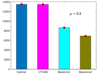
(a)

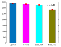
(b)

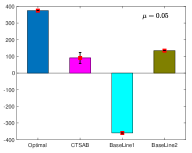
(c)

Figure 2: Comparison of cumulative reward of algorithm CTSAB with other policies for different mean value of the arm. We set $\epsilon=0.05$ and $\delta=0.05$

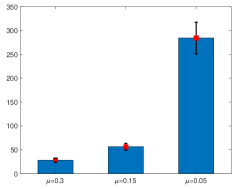
Figure 3: Regret of the CTSAB algorithm for the single arm problem as $\mu$ is varied.

References

• Abinav and Slivkins [2018] Karthik Abinav and Sankararaman Aleksandrs Slivkins. Combinatorial semi-bandits with knapsacks. In International Conference on Artificial Intelligence and Statistics (AISTATS), 2018.
• Agrawal and Devanur [2016] Shipra Agrawal and Nikhil R. Devanur. Linear contextual bandits with knapsacks. In Neural Information Processing Systems (NIPS 2016), 2016.
• Arora et al. [2019] Raman Arora, Teodor V. Marinov, and Mehryar Mohr. Bandits with feedback graphs and switching costs. In Advances in Neural Information Processing Systems(NIPS), 2019.
• Badanidiyuru et al. [2018] Ashwinkumar Badanidiyuru, Robert Kleinberg, and Aleksandrs Slivkins. Bandits with knapsacks. Journal of ACM, (13), 2018.
• Bubeck et al. [2012] Sébastien Bubeck, Nicolo Cesa-Bianchi, et al. Regret analysis of stochastic and nonstochastic multi-armed bandit problems. Foundations and Trends® in Machine Learning, 5(1):1–122, 2012.
• Cella and Cesa-Bianchi [2020] Leonardo Cella and Nicolò Cesa-Bianchi. Stochastic bandits with delay-dependent payoffs. In International Conference on Artificial Intelligence and Statistics, pages 1168–1177, 2020.
• Cesa-Bianchi et al. [2013] Nicola Cesa-Bianchi, Ofer Dekel, and Ohad Shamir. Online learning with switching costs and other adaptive adversaries. In Advances in Neural Information Processing Systems(NIPS), 2013.
• Combes et al. [2015] Richard Combes, Chong Jiang, and Rayadurgam Srikant. Bandits with budgets: Regret lower bounds and optimal algorithms. In International Conference on Measurement and Modeling of Computer Systems (SIGMETRICS), 2015.
• Dekel et al. [2014] Ofer Dekel, Jian Ding, Jian Ding, Tomer Koren, and Yuval Peres. Bandits with switching costs: $t2/3$ regret. In ACM Symposium on Theory of computing (STOC), pages 459 – 467, 2014.
• Ding et al. [2013] Wenkui Ding, Tao Qin Xu-Dong Zhang, and Tie-Yan Liu. Multi-armed bandit with budget constraint and variable costs. In Proceedings of the Twenty-Seventh AAAI Conference on Artificial Intelligence, 2013.
• Gong and Shroff [2019] Xiaowen Gong and Ness B Shroff. Truthful data quality elicitation for quality-aware data crowdsourcing. IEEE Transactions on Control of Network Systems, 7(1):326–337, 2019.
• Gopalakrishnan et al. [2016] Ragavendran Gopalakrishnan, Sherwin Doroudi, Amy R Ward, and Adam Wierman. Routing and staffing when servers are strategic. Operations research, 64(4):1033–1050, 2016.
• György et al. [2007] András György, Levente Kocsis, Ivett Szabó, and Csaba Szepesvári. Continuous time associative bandit problems. In IJCAI, pages 830–835, 2007.
• Hanawal et al. [2015a] Manjesh K. Hanawal, Amir Leshem, and Venkatesh Saligrama. Cost effective algorithms for spectral bandits. In IEEE International Conference on Acoustics, Speech and Signal Processing (ICASSP), pages 1323–1329, 2015a.
• Hanawal et al. [2015b] Manjesh K. Hanawal, Venkatesh Saligrama, Michal Valko, and Remi Munos. Cheap bandits. In International Conference on Machine Learning (ICML), 2015b.
• Immorlica et al. [2019] Nicole Immorlica, Karthik Abinav Sankararaman, Robert Schapire, and Aleksandrs Slivkins. Adversarial bandits with knapsacks. In Annual Symposium on Foundations of Computer Science (FOCS), 2019.
• Jun [2004] Tackseung Jun. A survey on the bandit problem with switching costs. In De Economist, page 513–541, 2004.