Examinations of CO completeness based on three independent CO surveys

Abstract

We report the global properties recovered by an ongoing CO survey of the Milky Way Imaging Scroll Painting (MWISP) toward the Galactic outskirts. Our results are also compared to those extracted by a uniform decomposition method from the CfA 1.2 m CO survey and the FCRAO 14 m outer Galaxy survey (OGS). We find that more extended and unseen structures are present in the MWISP data. The total flux across the disk recovered by the MWISP survey is 1.6 times larger than those recovered by the CfA and OGS surveys in the case of the same resolution. The discrepancies are scaling with distance. For example, in the outermost OSC arm, the flux ratios for MWISP-to-CfA and MWISP-to-OGS increase up to 43.8 and 7.4, respectively. Nonetheless, the census of molecular gas in our Galaxy is still far from complete by the MWISP, with flux completeness of $<$58%. The total mass ratios of the tabulated molecular clouds between different surveys are similar to the CO flux ratio. The application of these ratios to the total H₂ mass of our Galaxy yields a correction factor of at least 1.4, meaning that the H₂ mass of our Galaxy should be at least 40% more massive than previously determined. Including the completeness correction, an even more significant fraction of the matter should be contributed by baryonic matter. The mass spectrum in the outer Galactic plane is better described by a non-truncating power-law with $\gamma$=$-$1.83$\pm$0.05, and an upper mass of $M_{0}$=(1.3$\pm$0.5)$\times$10⁶ $M_{\sun}$.

1 Introduction

The $J$ = 1$\rightarrow$0 line of ¹²CO  is the most accessible and widely used tracer of the molecular interstellar medium due to the combination of high abundance and low permanent dipole moment (Bolatto et al., 2013; Heyer & Dame, 2015). As a consequence, most scientific time of the single-dish telescopes (e.g., the 1.2 m, the NANTEN 4 m, the Bell Laboratories 7 m, and the FCRAO 14 m telescopes) was devoted to the CO survey projects  (e.g., Heyer et al., 1998; Dame et al., 2001; Lee et al., 2001; Mizuno & Fukui, 2004; Jackson et al., 2006) since the discovery of the CO line in 1970. The major scientific achievements of the large CO surveys were summarized in a recent review by Heyer & Dame (2015). These CO surveys have been proved essential for improving our knowledge of the physics of molecular ISM, the physics of star formation, as well as the structure and dynamics of the Milky Way.

Benefit from the increasing of sensitivity, bandwidth, spectral channels, and enlarging of field of view by applying multi-beam receivers, more moderate- to large-size single-dish telescopes became capable of wide-field imaging of CO and its isotopologues, ¹³CO  and C¹⁸O. There are currently several new surveys being undertaken with new instruments equipped on the Mopra 22 m (e.g., Barnes et al., 2015, 2018), the Nobeyama 45 m (e.g., Umemoto et al., 2017), and the Purple Mountain Observatory (PMO) 13.7 m telescopes (e.g., Su et al., 2019). These new surveys allow at the same time high resolution, high sensitivity, and wide velocity coverage, enabling the examination of the internal structure of the clouds and the discovery of the faint and extended cloud envelopes, as well as the discovery of many new molecular clouds (MCs) with small angular size, and/or low surface brightness. Indeed, using the data from the ongoing project Milky Way Imaging Scroll Painting (MWISP) with the PMO 13.7 m telescope, we have detected many new MCs, and a new segment of the distant spiral arm (e.g., Sun et al., 2015; Su et al., 2016; Du et al., 2016; Sun et al., 2017), and have revealed the complex distribution of molecular material within the parent cloud (e.g., Zhang et al., 2014; Su et al., 2020; Lin et al., 2020).

While much scientific progress has been achieved from the analysis of CO survey data, our knowledge of the completeness of these CO surveys is still very limited. The observational effects on the cloud properties have long been known. For example, Rosolowsky & Leroy (2006) reported that the bias of measurements due to the observational effects is at least 40%. Based on the MWISP data ($l$ = [25$\fdg$8, 49$\fdg$7], and $b$=[$-$5$\fdg$25, +5$\fdg$25]), Yan et al. (2021b) investigated the dependence of observed properties of MCs (i.e., brightness temperature, flux) on angular resolution (beam sizes) and sensitivity by simulating observations with larger beam sizes and lower sensitivities. They found that the observed brightness temperature is mainly controlled by the resolution (beam size) of the observation. Rather low filling factors are reported for small clouds, i.e., only $\sim$50% for cloud with size of two resolution elements (Yan et al., 2021b). Furthermore, the flux completeness of a cloud strongly depends on the mean signal-to-noise ratio (S/N) of the cloud, which is about 0.5 for the case of S/N=3.3 (Yan et al., 2021b). All these findings strongly indicate that the census of molecular gas from the CO surveys with finite sensitivities and resolutions is mostly incomplete.

Currently, the region within Galactic coordinates $l$=[104$\fdg$75,150$\fdg$25] and $b$=[$-$5$\fdg$25,+5$\fdg$25] has been fully covered by the MWISP survey (Yan et al., 2021a), as well as partly covered by the FCRAO outer Galaxy CO survey (OGS; Heyer et al., 1998) and the CfA 1.2 m CO survey (Dame et al., 2001, hereafter the CfA survey). Such three independent surveys overlapped over a large area of the sky provide us an opportunity to investigate the completeness and limits of the CO surveys. The second quadrant contains four well-separated spiral arms along the line of sight. Thus it can additionally offer advantages over other Galactic quadrants when investigating the effects of distance. In this study, we investigate the recovered flux and its completeness measured by the CO surveys. This paper is organized as follows. First, the data and signal identification and decomposition methods are presented in Section 2, and in Section 3 the integrated cloud properties measured by the MWISP survey are presented along with a comparison with those measured by other surveys. Next, in Section 4 we discuss the lessons from the current CO surveys and the correction factor of total H₂ mass of our Galaxy. In Section 5 we summarize the results.

2 Data and analysis

This study is on the basis of the overlapped region of the MWISP, CfA, and OGS surveys, in the region of $l$ = [104$\fdg$75, 141$\fdg$54], $b$ = [$-$3$\fdg$028, 5$\fdg$007], and $V_{\rm LSR}$ = [$-$137, 40] km s^-1.

2.1 MWISP data

The MWISP project is an unbiased Northern Galactic Plane CO survey, which is capable of simultaneously observing J=1-0 ¹²CO, ¹³CO, and C¹⁸O lines (refer to Zhang et al., 2014; Sun et al., 2015; Su et al., 2019, etc., for project details and initial results). The MWISP CO data used here were observed during 2011 and 2020 with the PMO 13.7 m telescope. The front end detector was the Superconducting Spectroscopic Array Receiver (SSAR), a nine-beam, sideband-separating receiver (Shan et al., 2012). The angular resolution of the 13.7 m telescope is $\sim$50$\arcsec$ at the frequency of the ¹²CO(1-0) line. The on-the-fly (OTF) mode was applied in the MWISP survey. The sample spacing between adjacent scans is 15$\arcsec$ (see the details in Sun et al., 2018, for observation setups). Therefore, the MWISP survey fully sampled the mapped area. The OTF raw data were regridded into 30$\arcsec\times$30$\arcsec$ pixels. The total velocity coverage is $\sim$2600 km s^-1  with a channel width of 0.16 km s^-1. A first-order baseline correction was applied to the MWISP data. Please refer to Su et al. (2019) for details of the observation strategy and data reduction of the MWISP survey.

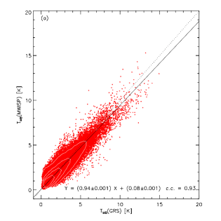
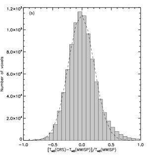
Figure 1: The ¹³CO(1-0) intensities from the MWISP survey by the PMO 13.7 m telescope and the GRS by the FCRAO 14 m telescope. The compared area is $l$=[29$\fdg$75, 40$\fdg$25], $b$=[$-$1$\fdg$0, +1$\fdg$0], and $V_{\rm LSR}$=[$-$5, 135] km s^-1. The two data sets are both smoothed to the same channel width of 2 km s^-1. We apply DBSCAN algotithm to identify signal. All voxels above 6$\sigma$ noise level are plotted. ($a$) The contours indicate number density of 2$\times$10², 2$\times$10³, 1$\times$10⁴, and 4$\times$10⁴, respectively. The solid-line shows the best-fit linear function of $T_{\rm MB}$(MWISP)=(0.94$\pm$0.001)$\times$$T_{\rm MB}$(GRS)+(0.08$\pm$0.001). The dotted-line shows the $T_{\rm MB}$(MWISP)=$T_{\rm MB}$(GRS). ($b$) Histogram of the difference between the valid voxel values of the two surveys. The dashed line shows the best fit of the distribution by a Gaussian function, with an offset of $-$0.014 and a standard deviation of 0.219.

The chopper-wheel calibration was adopted to get the antenna temperature, $T_{\rm A}^{*}$, which has been corrected for atmospheric absorption (Kutner & Ulich, 1981). Data presented in this paper are further converted to a scale of main beam brightness temperature, using $T_{\rm MB}$ = $T_{\rm A}^{*}\,$/$\eta_{\rm MB}$, where the main beam efficiency $\eta_{\rm MB}$ is typically 0.46 at 115 GHz (see the status report of the 13.7 m telescope ). Here, we verify the calibration accuracy of the MWISP data by comparing it with the FCRAO Galactic ring survey (GRS; Jackson et al., 2006). Because these two surveys are both fully sampled and have similar resolution and sensitivity, the difference of calibrated main beam temperature ($T_{\rm MB}$) would faithfully reflect the calibration uncertainty. Figure 1 shows the comparison results for the overlapped region of the two surveys, e.g., in the region of $l$=[29$\fdg$75, 40$\fdg$25], $b$=[$-$1$\fdg$0, +1$\fdg$0], and $V_{\rm LSR}$=[$-$5, 135] km s^-1. The two data sets are both smoothed to a same channel width of 2 km s^-1. The main beam temperatures of all voxels above 6$\sigma$ are pixel-by-pixel compared, which can be well fitted by a linear relation of $T_{\rm MB}$(MWISP)=(0.94$\pm$0.001)$\times$$T_{\rm MB}$(GRS)+(0.08$\pm$0.001), with a Pearson correlation coefficient of 0.93 (see Fig. 1a). The distribution of the fractional difference between all valid voxels, [$T_{\rm MB}$ (GRS)$-$$T_{\rm MB}$ (MWISP)]/$T_{\rm MB}$ (MWISP) is also plotted as a histogram. This distribution is fitted by a Gaussian function, with a peak of $-$0.014 and a width of 0.219. These indicate that calibration of the MWISP data is robust, and is consistent with that of the GRS data within $\sim$20%.

2.2 Archival Data

To date, the CO survey conducted with the CfA 1.2 m telescope is the only one that covers the whole Galactic plane (Dame et al., 2001). The CfA CO data used here were obtained during 1980 and 2001 (Dame et al., 2001). The angular resolution of the 1.2 m telescope is $\sim$8.5$\arcmin$. We used the raw data set where no interpolation was done. The publicly distributed CfA data are in units of $T_{\rm MB}$, where $\eta_{\rm MB}$ of 0.82 was used for correction. The pixel size of the whole data set is 7.5$\arcmin$, slightly less than one beam size. In the second Galactic quadrant, the velocity coverage of the survey is $\sim$$-$137 to $\sim$50 km s^-1  with a channel width of 1.3 km s^-1.

The OGS CO data used in this study are from Heyer et al. (1998), which were observed during 1994 and 1997 with the FCRAO 14 m telescope. These data, covering a Galactic coordinates range of $l$ = [102$\fdg$49, 141$\fdg$54] and $b$= [$-$3$\fdg$03, 5$\fdg$41], were sampled every 50$\arcsec$ with an angular resolution of $\sim$46$\arcsec$. The publicly distributed OGS data are in units of $T_{\rm R}^{*}$, corrected for forward spillover and scattering efficiency of the telescope, using $T_{\rm R}^{*}$ = $T_{\rm A}^{*}\,$/$\eta_{\rm FSS}$, where $\eta_{\rm FSS}$ is 0.7. We transform the OGS data to $T_{\rm MB}$ units, using $T_{\rm MB}$ = $T_{\rm R}^{*}\times$($\eta_{\rm FSS}\,$/$\eta_{\rm MB}$), where $\eta_{\rm MB}$ is 0.45. The velocity coverage is from $-$153 to 40 km s^-1  with a channel width of 0.81 km s^-1. Note that unlike the OTF mapping mode of the MWISP survey, the beam-by-beam mapping mode was applied in the CfA and OGS surveys. Therefore, these two surveys did not fully sample the mapped area.

Table 1: Summary of the survey data.

Survey	Beam size	Sampling	$V_{\rm LSR}$range	$\delta_{v}$	rms noisec	$\eta_{MB}$
			(km s-1)	(km s-1)	(K)
CfA 1.2 ma	8.5$\arcmin$	7.5$\arcmin$	[$-$137, +40]	1.3	0.07	0.82
OGSb	46$\arcsec$	50$\arcsec$	[$-$153, +40]	0.81	0.95	0.45
MWISP raw	50$\arcsec$	30$\arcsec$	$\sim$[-1400, +1200]	0.16	0.46	0.46
… smoothed1	…	50$\arcsec$	…	0.81	0.23	…
… smoothed2	8.5$\arcmin$	7.5$\arcmin$	…	1.3	0.04	…

Note. — ($a$) Dame et al. (2001). ($b$) Heyer et al. (1998). ($c$) The rms noise are in units of $T_{\rm MB}$

2.3 Signal Identification and Decomposition

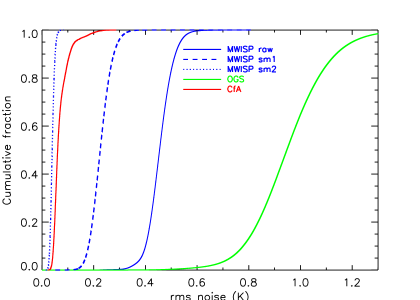
Figure 2: The cumulative distributions of $\sigma$ for ¹²CO  emission from the MWISP (blue), OGS (green), and CfA 1.2 m (red) surveys within the region of $l$=[104$\fdg$75, 141$\fdg$54] and $b$=[$-$3$\fdg$028, +5$\fdg$007]. The solid lines are derived from the raw data. The dashed-blue and dotted-blue lines are derived from the smoothed MWISP data with the same resolution and sampling as the OGS and CfA surveys, respectively.

We estimate the noises of each data set by measuring the rms intensity, $\sigma_{\rm rms}$, from the signal-free channels of the data cube. The mean values of $\sigma_{\rm rms}$ are 0.46 K, 0.95 K, and 0.07 K for the data sets of the MWISP, OGS, and CfA surveys with full resolution, respectively. The MWISP data are also convolved and regridded to match the resolutions and sample spacings of the CfA and OGS surveys. The spatial smoothing operation is performed with the Python package spectral-cube . The corresponding $\sigma_{\rm rms}$ for the smoothed MWISP data have mean values of 0.04 K, and 0.23 K, which are larger than predicted by theory. Further investigations are needed to understand these discrepancies. The cumulative distributions of $\sigma_{\rm rms}$ for the five data sets of the three CO surveys are shown in Figure 2.

The simplest method for signal identification is “clipping”, in which all voxels with intensities above some statistical significance level are judge to be real signals. But we often find ourselves in a dilemma when choosing an optimum intensity level. A loose criterion could not significantly suppress the noise, while a strict criterion might filter a substantial amount of real emission. Therefore, we adopted a more sophisticated approach developed by Yan et al. (2020) to identify regions of contiguous, significant emission in the position-position-velocity (PPV) data cubes. This approach is based on the density-based spatial clustering of applications with noise (DBSCAN) algorithm . This algorithm contains three free parameters: (1) MinPts which defines the minimum number of voxels of the structure, (2) $\epsilon$ which defines the neighborhood of voxels, and (3) $T_{\rm cutoff}$ which defines the boundary isosurface of the structure (Yan et al., 2020). Many combinations of parameters were made before finalizing on MinPts=4, $\epsilon$=1, and $T_{\rm cutoff}$=2$\sigma$. Such choice of parameters can identify most of the significant emission (including both the compact and the extended emission). The definition of connected regions of emission in PPV space here is generally consistent with the trunks defined by dendrogram algorithm (Rosolowsky et al., 2008).

Post selection was also recommended by Yan et al. (2020) to ensure including as few noise clouds as possible. In this step, a cloud was further rejected from the raw catalogs if any one of the following criteria is met: (1) the voxel number below 16, (2) peak brightness temperature below 5$\sigma$, (3) projection area has no compact 2$\times$2 region, and (4) channel number less than 3. We then construct a mask according to the signal identification results, which was applied to the raw data cubes. The emission-free voxels are blanked. The masked versions of data cubes are used for the following analysis.

3 Results

3.1 Large-scale Structure Traced by CO

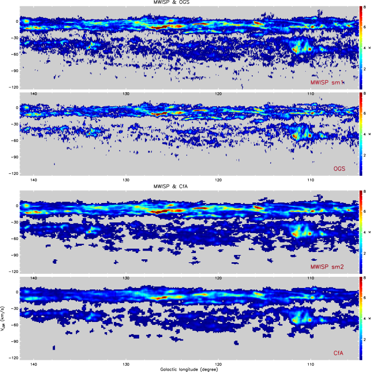
Figure 3: The longitude-velocity maps integrated over Galactic latitude range of $b$ = $-$3$\fdg$028 to 5$\fdg$007. The MWISP data are smoothed to match the resolution and sampling of the OGS and CfA surveys. The images only contain emission identified by DBSCAN. All emission-free pixels are blanked.

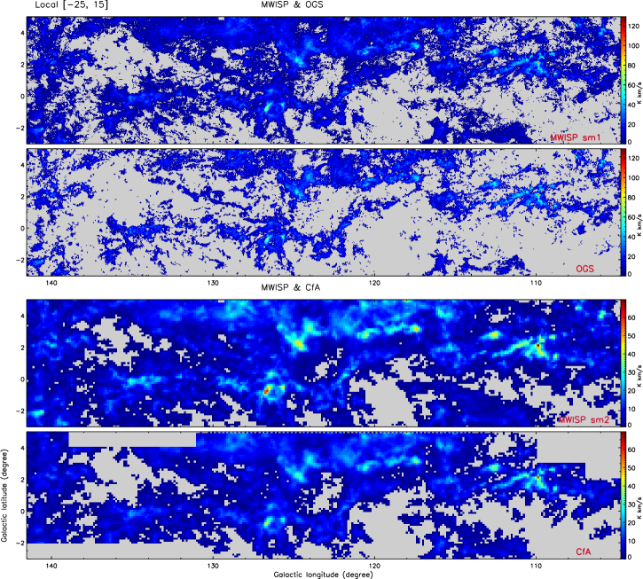
Figure 4: Integrated intensity maps of ¹²CO  emission. The velocity range is marked in the corner of each map. The MWISP data are smoothed to match the resolution and sampling of the OGS and CfA surveys. The images only contain emission identified by DBSCAN. All emission-free pixels are blanked.

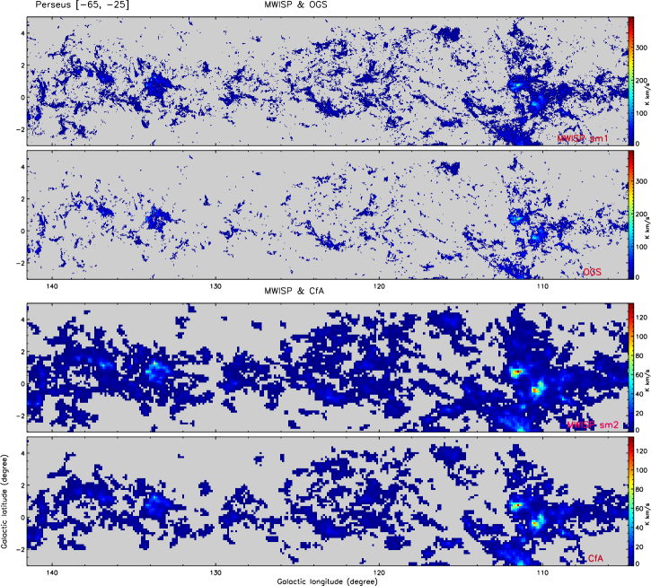
Figure 4: (Continued).

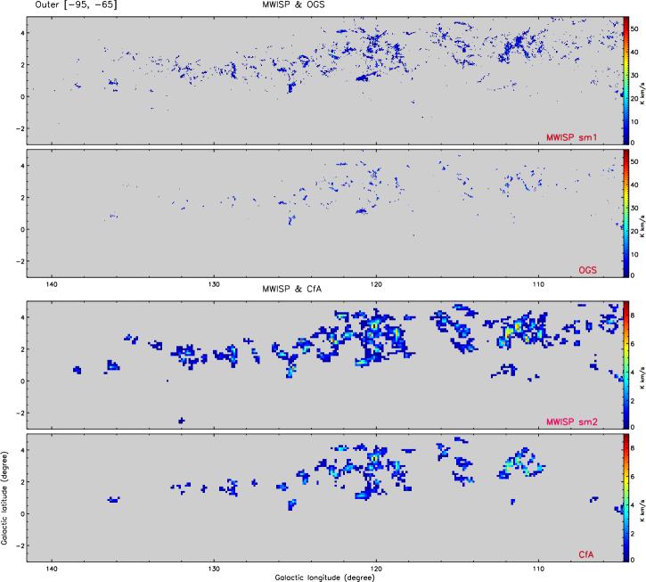
Figure 4: (Continued).

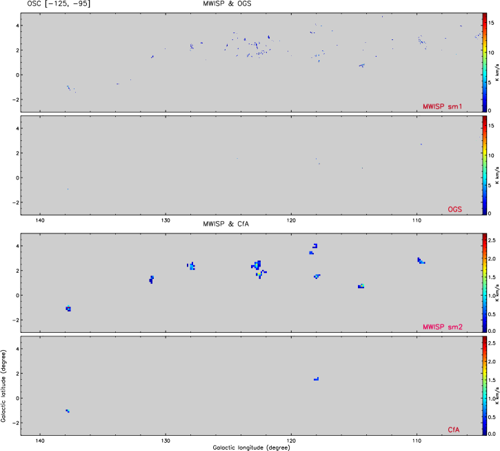
Figure 4: (Continued).

Figure 3 presents the longitude-velocity ($l$-$v$) maps integrated over $b$ = [$-$3$\fdg$028, 5$\fdg$007], which are derived from the noise-suppressed data cubes of the three surveys. The integrated intensity maps of the four spiral arms derived from the three surveys are also compared in Figure 4. Note that the maps derived from the MWISP data with the full resolution and the same resolution as the OGS are almost identical by human eyes, thus the maps derived from the former are not displayed here. Compared with the moment masked $l$-$v$ map of the CfA (Fig. 3 of Dame et al., 2001) and the unmasked map of the OGS (Fig. 4 of Heyer et al., 1998), the structures shown in their $l$-$v$ maps are generally consistent with those revealed in Fig. 3. Examined more closely, however, there are some weaker features at the large negative velocity newly recovered in Fig. 3. We find that these distant features were actually judged to be real MCs by Digel et al. (1994) and Miville-Deschênes et al. (2017). The comparison confirms that the DBSCAN performs as well as the often used moment mask method. Moreover, our choice of parameters assures a reliable extraction of CO emission, even at a low S/N ratio.

The features revealed by the three independent surveys are also compared. We find that all data sets with a variety of resolutions and sensitivities have the ability to resolve major features of the Local arm from $\sim-$25 to $\sim$15 km s^-1and the Perseus arm from $\sim-$65 to $\sim-$25 km s^-1, due to their relatively small distances and/or large angular sizes. And as expected, the internal sub-structure within each arm can only be well resolved by the ones with higher resolution (e.g., the OGS and MWISP surveys). The Outer arm ($\sim-$95 to $\sim-$65 km s^-1) appears as a more coherent feature in the MWISP survey than in the other two surveys. Besides, the MWISP data discover a new component lying beyond the Outer arm at the maximum negative velocity (at $V_{\rm LSR}$$<\sim-$95 km s^-1, namely the Outer Scutum-Centaurus arm, hereafter OSC), which was firstly reported in our previous work (Sun et al., 2015). Some new features with small angular size and/or relatively faint emission are also emerging between each pair of adjacent arms by the MWISP survey. Considering that these features are extracted by a uniform approach, these discrepancies would faithfully reflect the observational effects introduced by the finite sensitivity and resolution of each survey. Our lesson from such a rough comparison is that the survey with both high sensitivity and resolution will offer complementary or new insights into the spiral structure in outer or extreme outer Galaxy regions, the internal structure within each spiral arm, and the inter-arm structure between each pair of adjacent arms.

3.2 Voxel Number and Flux Recovered

The integrated flux of CO emission represents an essential parameter because it can be well translated into total H₂ gas mass. Therefore it is investigated in detail in the following two sections. The total voxel number can reflect the volume of the CO emission region in the PPV space. Thus it is also investigated. Table 2 summarizes the total numbers of voxels (Cols. 2-6), total fluxes (Cols. 7-11) recovered by the five data sets, the voxel number ratios and the flux ratios of MWISP-to-OGS (Cols. 12-13), and MWISP-to-CfA (Cols. 14-15) in the case of full resolution and same resolution, respectively. Here the total flux is simply the integration of all the emission: F= $\Sigma_{i}\,T_{i}\delta\theta_{x}\delta\theta_{y}\delta\,v$.

We find that the voxel number and flux recovered by the MWISP survey are always the largest. In the case of different resolutions, the voxel number ratio is meaningless and thus is not compared here. The total flux recovered by the raw MWISP survey is about 1.3 times larger than that of the OGS survey and 1.1 times larger than that of the CfA survey. Even considering the uncertainty possibly introduced by calibration, with typically of 10%, the difference between the MWISP and OGS surveys is still significant. To better understand which factor is dominant in the discrepancy, we also compared the results identified by surveys with the fixed resolutions but different sensitivities. We find that the total fluxes recovered by the smoothed MWISP data sets (Cols. 8-9) are somewhat larger than that from the raw data (Col. 7). Naturally, the total flux ratios of MWISP-to-OGS and MWISP-to-CfA are both shifted to an even higher value of 1.6 in the case of the same resolution.

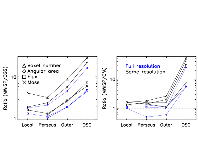
Figure 5: ($a$) The voxel number ratio, flux ratio, projected area ratio, mass ratio of MWISP-to-OGS in the case of full resolution (plotted in blue) and same resolution (plotted in black). ($b$) Same as panel ($a$), but for the ratio of MWISP-to-CfA.

As previously mentioned, the ¹²CO  observation covers a large range of volumes of the Milky Way (out to Galactocentric radii of $R$=$\sim$25 kpc). The observational effects would be expected to increase with distance as decreasing the detection limits of the cloud size and mass. Thus, we also examine the statistical results across the four spiral arms roughly defined according to the $V_{\rm LSR}$  distribution (mentioned in § 3.1). Note that the inter-arm regions are ignored here given their negligible contributions. It is obvious that both the voxel number and flux drop rapidly beyond the Perseus arm, which differs by several orders of magnitude in different arms. This is particularly severe by the CfA and OGS survey. Consequently, the voxel number ratios and flux ratios rise to as high as 27.9 and 7.4 for MWISP-to-OGS, and 53.3 and 43.8 for MWISP-to-CfA in the farthest OSC arm. In addition, we see that the voxel number ratios are always larger than the flux ratios for all arm components. The voxel number ratios and flux ratios across the four spiral arms are also shown in Figure 5.

Table 2: Total number of voxel and total flux recovered.

Arm	Total voxel						Total flux						Voxel ratio&Flux ratio
	MWISP			OGS	CfA		MWISP			OGS	CfA		MWISP/OGS			MWISP/CfA
	raw	sm1	sm2	raw	raw		raw	sm1	sm2	raw	raw		raw	sm1		raw	sm2
(1)	(2)	(3)	(4)	(5)	(6)		(7)	(8)	(9)	(10)	(11)		(12)	(13)		(14)	(15)
All	4.2e7	5.4e6	1.5e5	1.4e6	9.0e4		5.2e6	6.3e6	7.7e6	3.9e6	4.9e6		–&1.3	3.9&1.6		–&1.1	1.7&1.6
Loc	3.2e7	4.2e6	1.1e5	1.0e6	6.7e4		3.9e6	4.7e6	5.9e6	2.7e6	3.7e6		–&1.4	4.2&1.7		–&1.1	1.6&1.6
Per	8.6e6	1.1e6	3.7e4	3.3e5	2.1e4		1.3e6	1.5e6	1.7e6	1.1e6	1.2e6		–&1.2	3.3&1.4		–&1.1	1.8&1.4
Out	5.0e5	8.8e4	4.2e3	1.0e4	1.6e3		4.9e4	6.7e4	1.0e5	2.5e4	5.0e4		–&2.0	8.8&2.7		–&1.0	2.6&2.0
OSC	1.8e4	3.9e3	1.6e2	1.4e2	3.0		1.7e3	2.6e3	2.8e3	3.5e2	6.4e1		–&4.9	27.9&7.4		–&26.6	53.3&43.8

Note. — Columns (2)-(6): total number of voxels recovered by the raw MWISP survey, the MWISP survey with the same resolutions as the OGS and CfA surveys, the raw OGS and CfA surveys, respectively. Columns (7)-(11): total flux of the recovered voxels, in units of K km s^-1 arcmin². Columns (12)-(13): voxel ratio and flux ratio of MWISP/OGS, with the original resolution and same resolution, respectively. Columns (14)-(15): voxel ratio and flux ratio of MWISP/CfA, with the original resolution and same resolution, respectively.

3.3 Completeness of the Flux

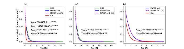
Figure 6: The total flux recovered as a function of main beam temperature, $T_{\rm cutoff}$ for the MWISP (blue), OGS (green), and CfA (red) surveys. The MWISP data are also smoothed to match the resolution and sampling of the OGS data (middle panel), and the CfA data (right panel), respectively.

The fluxes recovered, $F\,$($>$$T_{\rm MB}$), by each survey above a given main beam temperature, $T_{\rm MB}$, are plotted in Figure 6, both in the case of the original resolution and sampling (left panel) and the same resolution and sampling (middle and right panels). The values of $T_{\rm MB}$ range from $T_{\rm MB}=$3$\sigma_{\rm rms}$  (near the lowest cloud boundary as defined in §2.3, that is, sensitivity limit) to the peak temperature of the cloud, $T_{\rm peak}$. To some extent, the high end $T_{\rm MB}$ is mainly affected by the resolutions and sampling of the observations, and we would expect its distribution to move to somewhat higher values of $T_{\rm peak}$ with observations characterized by better resolutions and sampling. Indeed, the MWISP and OGS surveys with higher resolutions have much higher dynamic ranges of $T_{\rm MB}$ than the CfA survey. In addition, we find that at a given $T_{\rm MB}$, the fluxes $F\,$($>$$T_{\rm MB}$) recovered by the MWISP survey are larger than those by the CfA survey, while are slightly less than those by the OGS survey even compared under the same angular and velocity resolutions.

Table 3: Flux completeness.

Arm	Parameter $a$						Parameter $b$						Completeness
	MWISP			OGS	CfA		MWISP			OGS	CfA		MWISP
	raw	sm1	sm2	raw	raw		raw	sm1	sm2	raw	raw		raw	sm1	sm2
(1)	(2)	(3)	(4)	(5)	(6)		(7)	(8)	(9)	(10)	(11)		(12)	(13)	(14)
All	9.0e6	8.3e6	8.2e6	1.0e7	5.9e6		0.38	0.38	0.58	0.34	0.87		0.58	0.75	0.94
Loc	7.5e6	6.7e6	6.4e6	9.7e6	4.6e6		0.44	0.44	0.62	0.42	0.95		0.52	0.71	0.91
Per	1.8e6	1.7e6	1.7e6	2.0e6	1.2e6		0.25	0.25	0.52	0.22	0.63		0.70	0.85	1.01
Out	1.3e5	1.2e5	1.2e5	1.0e5	9.9e4		0.70	0.72	2.17	0.50	3.10		0.38	0.61	0.80
OSC	5.3e3	5.3e3	6.0e3	1.2e3	1.9e2		0.84	0.95	6.51	0.43	5.00		0.32	0.54	0.44

Note. — We fit the $F\,$($>$$T_{\rm MB}$)-$T_{\rm MB}$ relation with an exponential function, $F\,$($>$$T_{\rm MB})=a\,{\rm exp}(-bT_{\rm MB})$, where $a$ and $b$ are two parameters. The derived values for $a$ and $b$ are summarized in Columns (2)-(6) and Columns (7)-(11), respectively. The flux completeness, $F\,$($>$3$\sigma$)/$F\,$($>$0), for the MWISP survey with the original resolution (Col. 12) and same resolutions as the OGS (Col. 13) and CfA (Col. 14) surveys are also tabulated.

Figure 6 shows a nonlinear falling of $F\,$($>$$T_{\rm MB}$) with $T_{\rm MB}$ for all data sets, which can be approximately described by an exponential function, $F\,$($>$$T_{\rm MB})=a\,{\rm exp}(-b\,T_{\rm MB})$, where $a$ and $b$ are two parameters. $a$ is equivalent to the flux that we would expect to measure with perfect sensitivity (a theoretical $T_{\rm MB}$=0 K isosurface). A larger value of $b$ implies a faster decreasing of $F\,$($>$$T_{\rm MB}$) with $T_{\rm MB}$. We use curve_fit in the Python package SciPy to fit the distribution, with flux errors considered. The error of recovered flux is estimated with $\sqrt{N}\sigma$, where $N$ is the voxel number, and $\sigma$ is the rms noise of each voxel. The derived relations are marked in each panel, which are apparently different across a variety of data sets. The values of $a$ and $b$ both seem to strongly depend on the spectral and spatial resolutions of the data. Indeed, when different data sets are smoothed to the same resolution, consistent values of both $a$ and $b$ are derived (refer to middle and right panels of Fig. 6). To avoid chaos, only the exponential fitting results to the MWISP data are overlapped.

Using these relations, we can also extrapolate the flux to the $T_{\rm MB}$=0 K isosurface. Hence, the completeness of flux can be calculated by the ratio of the flux at 3$\sigma$ cutoff, $F\,$($>$3$\sigma$), and the expected flux given infinite sensitivity, $F\,$($>$0 K). We see that the estimated flux completeness is also suffered observational effects, as higher expected values of $F\,$($>$0 K), while somewhat lower values of $F\,$($>$3$\sigma$) are found in the data sets with higher resolutions. Thus the corresponding completeness estimated here might only represent an upper limit, particularly in the data set with relatively coarse resolution, at which the majority of clouds are commonly marginally resolved or detected.

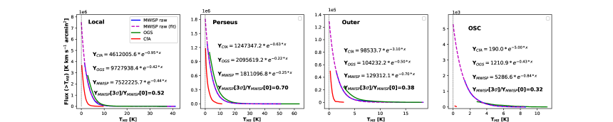
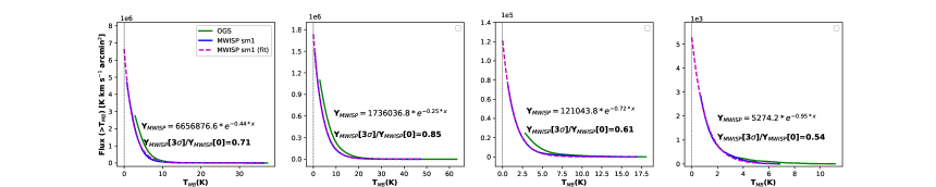
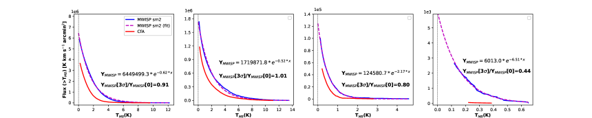
Figure 7: Same as Fig. 6 but for different spiral arms that are roughly defined according to the $V_{\rm LSR}$  distributions: (1) the Local arm [$-$25, 15 km s^-1], (2) the Perseus arm [$-$65, $-$25 km s^-1], (3) the Outer arm [$-$95, $-$65 km s^-1], and (4) the OSC arm [$-$125, $-$95 km s^-1].

The flux recovered and flux completeness are also investigated in the four spiral arms with different Galactocentric radii (refer to Fig. 7). In the top panel, the results are derived from data with the original resolution and sampling. In comparison, the middle and bottom panels are in the case of the same resolution and sampling. We see that the conclusions drawn from the whole region in Fig. 6 are still valid in these four sub-regions. The MWISP and OGS data have a similar $b$ value for a given arm component, which is smaller than that of the CfA data. We find that the value of $b$ parameter seems to increase rapidly beyond the Perseus arm, which implies a rapid falling of $F\,$($>$$T_{\rm MB}$) with $T_{\rm MB}$. As expected, the flux recovered is less complete in the more distant spiral arm, which is only 32% in the OSC arm, even by the MWISP survey. It is important to note that the estimation only represents a lower limit, as previously discussed. The derived $F\,$($>$$T_{\rm MB})$-$T_{\rm MB}$ relations and the flux completeness are all summarized in Table 3.

3.4 Recovered Molecular Clouds and Their Area and Mass

In the following two subsections, the molecular gas properties are derived based on MC samples, i.e., the whole sample and the sub-samples in the four individual spiral arms. MCs are assigned to each spiral arm based on $V_{\rm LSR}$ range as mentioned in § 3.1. We use the parallax-based distance estimator of Reid et al. (2019) to determine the distance to each cloud. Given the large uncertainties of kinematic distances to the MCs in the Local arm, these MCs are excluded in the following analysis. The typical distances for the whole sample and the three sub-samples are summarized in Table 4. The molecular gas masses are derived by assuming a constant CO-to-H₂ conversion factor of 2.0$\times$10²⁰ cm${}^{\rm-2}{\rm(K\,km\,s^{-1})^{-1}}$ (Bolatto et al., 2013). Following Yan et al. (2020), the MC’s properties are measured. Table 5 summarizes the total number of MCs (Cols. 2-6), the total projected angular area of MCs (Cols. 7-11), the total mass of MCs (Cols. 12-16), and the area ratio and mass ratio (Cols. 17-20) that recovered by the five data sets of the three surveys.

Table 4: Summary of the molecular cloud distances.

	Median						Mean						S.D.
	MWISP			OGS	CfA		MWISP			OGS	CfA		MWISP			OGS	CfA
	raw	sm1	sm2	raw	raw		raw	sm1	sm2	raw	raw		raw	sm1	sm2	raw	raw
(1)	(2)	(3)	(4)	(5)	(6)		(7)	(8)	(9)	(10)	(11)		(12)	(13)	(14)	(15)	(16)
All	2.67	2.69	2.69	2.67	2.66		3.35	3.53	3.90	3.05	3.33		1.79	1.93	2.41	1.35	1.92
Per	2.64	2.64	2.54	2.66	2.62		2.77	2.80	2.71	2.76	2.67		0.87	0.92	0.87	0.81	0.72
Out	5.96	6.06	6.24	6.05	5.96		5.96	6.24	6.54	5.78	6.20		1.64	1.22	1.32	1.59	1.42
OSC	10.36	10.29	10.29	10.57	17.37		10.63	10.60	10.58	11.38	17.37		1.74	1.82	2.58	2.34	–

Note. — The statistical parameters for MC’s distance (in units of kpc) are summarized, including the median value (Columns 2-6), mean value (Columns 7-11), and standard deviation (Columns 12-16) for the MWISP raw data, same resolutions as OGS and CfA surveys, raw OGS and CfA surveys, respectively.

Table 5: Summary of the molecular cloud properties.

Arm	Total number						Total area						Total mass						Area ratio&Mass ratio
	MWISP			OGS	CfA		MWISP			OGS	CfA		MWISP			OGS	CfA		MWISP/OGS			MWISP/CfA
	raw	sm1	sm2	raw	raw		raw	sm1	sm2	raw	raw		raw	sm1	sm2	raw	raw		raw	sm1		raw	sm2
(1)	(2)	(3)	(4)	(5)	(6)		(7)	(8)	(9)	(10)	(11)		(12)	(13)	(14)	(15)	(16)		(17)	(18)		(19)	(20)
All	7368	4599	221	1946	156		65.0	75.0	1.9e2	27.0	1.2e2		5.2e6	6.1e6	5.6e6	4.2e6	4.0e6		2.4&1.3	2.7&1.5		0.5&1.3	1.6&1.4
Per	6231	3752	163	1773	130		57.8	65.9	1.7e2	26.0	1.1e2		4.3e6	4.8e6	4.6e6	3.7e6	3.2e6		2.2&1.1	2.5&1.3		0.5&1.3	1.6&1.4
Out	1007	747	48	165	25		6.6	8.2	19.7	1.4	1.2e1		8.4e5	1.2e6	8.1e5	4.2e5	7.4e5		4.8&2.0	6.0&2.9		0.5&1.1	1.6&1.1
OSC	130	100	10	8	1		0.4	0.6	2.5	0.02	0.08		1.2e5	1.6e5	1.6e5	2.6e4	2.1e4		19.4&4.6	26.1&6.1		5.5&5.6	31.8&7.6

Note. — Columns (2)-(6): total number of objects recovered by the MWISP data with original resolution, same resolutions as OGS, and CfA surveys, raw OGS and CfA surveys, respectively. Columns (7)-(11): the total projected area of the recovered objects, in units of deg². Columns (12)-(16): the total mass of the recovered objects, in units of $M_{\sun}$. Columns (17)-(18): area ratio and mass ratio of MWISP/OGS, with the original resolution and same resolution, respectively. Columns (19)-(20): area ratio and mass ratio of MWISP/CfA, with the original resolution and same resolution, respectively.

We find that the number of molecular clouds identified by the MWISP survey with the full resolution is up to $\sim$2 orders of magnitude larger than that of the CfA survey, and $\sim$3 times larger than that of the OGS survey. Such significant discrepancy is perhaps not surprising because the recovered objects are controlled by the sensitivity and resolution of the data set. As stated in § 2.3, regions of emission could be successfully recovered as single entities only if their sizes are larger than the resolutions of the observations, the separations of the blend sources are larger than the resolutions, and their brightness temperatures are above a user-defined threshold. Additionally, the sensitivity of the data set that defines the boundary of the molecular cloud also has somewhat effects on the decomposition results, because the higher sensitivity data would tend to merge multiple MCs into a single MC. When MWISP data are smoothed and resampled to the resolutions and pixel sizes of the OGS and CfA surveys, we find that comparable numbers of clouds to the OGS and CfA surveys are identified in these smoothed MWISP data, with values of 8133 and 286.

The total projected area of MCs recovered by the raw MWISP is 2.0 times larger than that recovered by the OGS survey, but is only 80 per cent of that recovered by the CfA survey. Here the deconvolution is performed by subtracting the beam from the measured projected area. It seems that the smoothing of the MWISP data to the OGS velocity resolution does not significantly change the projected area recovered (75 deg² that is similar to the raw MWISP). Thus the area ratio of the smoothed MWISP to OGS almost remains unchanged as compared to that of the raw data. However, the smoothing of the MWISP to the CfA resolution produces a significant boost of projected area recovered (up to 190 deg² that is 2.9 times larger than that of the raw MWISP), as a consequence, the area ratio of the smoothed MWISP to CfA increases up to 1.6.

As expected, the total molecular gas mass of the MCs recovered by the MWISP is the highest, which is 1.5 and 1.4 times those recovered by the OGS and CfA surveys in the case of the full resolution, respectively. We also examine the statistical results recovered across the three sub-samples. It shows that the number, projected area, and mass of the clouds recovered all decrease rapidly beyond the Perseus arm, particularly significant in results recovered by the CfA and OGS surveys. As a consequence, the area ratios and mass ratios of MWISP-to-CfA and MWISP-to-OGS rise with increasing distance (plotted in Fig. 5).

3.5 Distributions of physical parameters

Table 6: Statistical parameters of the molecular cloud physical size.

	Min						Max						Median						Mean
	MWISP			OGS	CfA		MWISP			OGS	CfA		MWISP			OGS	CfA		MWISP			OGS	CfA
	raw	sm1	sm2	raw	raw		raw	sm1	sm2	raw	raw		raw	sm1	sm2	raw	raw		raw	sm1	sm2	raw	raw
(1)	(2)	(3)	(4)	(5)	(6)		(7)	(8)	(9)	(10)	(11)		(12)	(13)	(14)	(15)	(16)		(17)	(18)	(19)	(20)	(21)
All	0.3	0.6	6.4	0.7	5.4		64.8	75.2	170.1	40.3	138.5		1.3	1.9	16.4	1.8	14.7		2.0	2.9	23.6	2.5	19.9
Per	0.3	0.6	6.4	0.7	5.4		64.8	75.2	170.1	40.3	138.5		1.1	1.6	12.3	1.7	11.8		1.7	2.4	18.0	2.4	16.5
Out	0.5	1.0	10.4	1.1	14.6		31.4	57.6	101.6	14.6	78.0		2.7	3.7	33.9	3.7	33.6		3.6	5.0	36.6	4.5	36.3
OSC	1.9	2.1	26.2	4.0	47.8		24.4	27.3	76.3	10.9	47.8		4.6	6.4	51.5	5.4	47.8		5.3	7.2	51.1	5.9	47.8

Note. — The statistical parameters for MC’s size (in units of pc) are summarized, including the minimum (Columns 2-6), maximum (Columns 7-11), median (Columns 12-16), and mean (Columns 17-21) values, for the MWISP raw data, same resolutions as OGS and CfA surveys, raw OGS and CfA surveys, respectively.

Table 7: Statistical parameters of the molecular cloud mass.

	Min						Max						Median						Mean
	MWISP			OGS	CfA		MWISP			OGS	CfA		MWISP			OGS	CfA		MWISP			OGS	CfA
	raw	sm1	sm2	raw	raw		raw	sm1	sm2	raw	raw		raw	sm1	sm2	raw	raw		raw	sm1	sm2	raw	raw
(1)	(2)	(3)	(4)	(5)	(6)		(7)	(8)	(9)	(10)	(11)		(12)	(13)	(14)	(15)	(16)		(17)	(18)	(19)	(20)	(21)
All	1.0	6.4	1.4e2	25.0	2.7e2		1.1e6	1.3e6	2.6e6	5.9e5	1.9e6		34.0	95.0	2.8e3	2.7e2	3.2e3		7.1e2	1.3e3	2.5e4	2.1e3	2.6e4
Per	1.0	6.4	1.4e2	25.0	2.7e2		1.1e6	1.3e6	2.6e6	5.9e5	1.9e6		26.0	66.0	1.5e3	2.4e2	2.2e3		6.8e2	1.3e3	2.8e4	2.1e3	2.5e4
Out	2.7	19.0	9.3e2	55.0	2.0e3		6.6e4	1.9e5	1.7e5	4.1e4	1.6e5		1.2e2	2.9e2	7.4e3	9.4e2	1.8e4		8.3e2	1.6e3	1.7e4	2.5e3	3.0e4
OSC	34.0	1.0e2	5.6e3	9.1e2	2.1e4		2.3e4	2.9e4	4.8e4	1.0e4	2.1e4		3.1e2	7.9e2	1.3e4	1.8e3	2.1e4		9.1e2	1.6e3	1.6e4	3.2e3	2.1e4

Note. — The statistical parameters for MC’s mass (in units of $M_{\sun}$) are summarized, including the minimum (Columns 2-6), maximum (Columns 7-11), median (Columns 12-16), and mean (Columns 17-21) values, for the MWISP raw data, same resolutions as OGS and CfA surveys, raw OGS and CfA surveys, respectively.

Table 8: Statistical parameters of the molecular cloud surface density.

	Min						Max						Median						Mean
	MWISP			OGS	CfA		MWISP			OGS	CfA		MWISP			OGS	CfA		MWISP			OGS	CfA
	raw	sm1	sm2	raw	raw		raw	sm1	sm2	raw	raw		raw	sm1	sm2	raw	raw		raw	sm1	sm2	raw	raw
(1)	(2)	(3)	(4)	(5)	(6)		(7)	(8)	(9)	(10)	(11)		(12)	(13)	(14)	(15)	(16)		(17)	(18)	(19)	(20)	(21)
All	1.5	2.5	0.8	10.7	2.0		82.4	73.9	28.4	256.9	32.0		6.2	7.6	2.8	26.2	4.7		7.9	9.3	3.7	29.9	5.7
Per	1.5	2.5	0.8	10.7	2.0		82.4	73.9	28.4	256.9	32.0		6.4	7.9	3.1	26.5	5.0		8.2	9.7	4.0	30.4	6.0
Out	1.8	3.0	0.8	13.2	2.4		27.9	27.4	10.5	66.1	9.0		5.6	6.7	2.4	23.7	4.2		6.5	7.5	3.0	24.9	4.7
OSC	2.3	3.1	0.8	16.3	2.9		21.9	20.1	2.6	34.8	2.9		5.1	6.0	1.6	26.2	2.9		6.1	7.0	1.8	25.0	2.9

Note. — The statistical parameters for MC’s surface density (in units of $M_{\sun}$ pc^-2) are summarized, including the minimum (Columns 2-6), maximum (Columns 7-11), median (Columns 12-16), and mean (Columns 17-21) values, for the MWISP raw data, same resolutions as OGS and CfA surveys, raw OGS and CfA surveys, respectively.

The statistical parameters for MC’s size, mass, mass surface density are summarized in Tables 6-8, including the minimum, maximum, median, and mean values for each property. We find that all parameters presented here are different between the five data sets, which seem to be controlled by the data quality and the distance to MC. As expected, the MWISP MC sample shows the lowest statistical values of mass surface density, as MWISP data are capable of detecting faint emission around the periphery of the cloud and a large number of small and faint clouds that were largely missed by previous surveys.

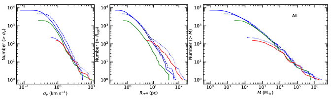
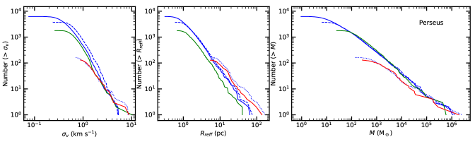
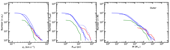
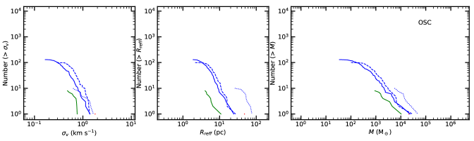
Figure 8: The cumulative distributions of velocity dispersion, effective radius, and mass of the molecular clouds that extracted from the MWISP (blue), OGS (green), and CfA (red) surveys. The blue-, green-, and red-solid lines indicate the results from the MWISP, OGS, and CfA raw data, respectively. The blue-dashed and blue-dotted lines indicate results from the smoothed MWISP data with the same resolution as the OGS and CfA data, respectively. 

Figure 8 presents the cumulative distributions of the velocity dispersion ($\sigma_{\rm v}$), effective radius ($R_{\rm eff}$), and mass ($M$) for the molecular clouds extracted from the five data sets. Both the whole cloud sample, and the sub-samples in the Perseus, Outer, and OSC arms are compared. For a better comparison, each property is plotted in figures with a fixed range of scale. It shows that both the dynamic range of each property and the shape of each distribution are significantly different between the five data sets of the three surveys across the Galactic disk. The dynamic ranges of all these three fundamental properties exhibit the largest range in the MWISP data, while the smallest range in the CfA data. It seems that those small or fain MCs could only be detected by those surveys with high resolution and high sensitivity. We quantify the difference by applying both a truncated power-law function, $N(x>x{{}^{\prime}})=N_{0}[(x/x_{0})^{\gamma+1}-1]$, and a non-truncated power-law function, $N(x>x{{}^{\prime}})=[(x/x_{0})^{\gamma+1}]$ (e.g., Heyer & Dame, 2015; Rice et al., 2016; Colombo et al., 2019) to the cloud size and mass distributions. Here the completeness limits are evaluated by the mean size and mean mass of objects recovered by each data set (refer to Tables 6-7), which represent conservative estimations.

Using the maximum-likelihood method of Rosolowsky (2005) and Rosolowsky (2007), the size and mass spectra are measured. We find that the size and mass distributions in the outer Galaxy are better fitted by non-truncated power-law functions in most situations. The only exception is the size spectrum of the whole cloud sample extracted from the raw MWISP data, which can not be well fitted at the high-value end. The MCs’ size function fitting results for the different data sets and different distance components are summarized in Table 9. Similarly, the MCs’ mass function fitting results are summarized in Table 10. Note that the fitting results for clouds number below 10 have large uncertainties thus are not fitted here.

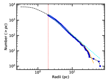
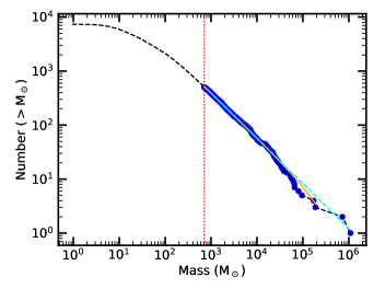
Figure 9: Cumulative effective radius (left) and mass (right) functions for the whole cloud sample extracted from the raw MWISP data. In each panel, both a truncated (solid orange) and a non-truncated (dashed cyan) power-law spectrum are fit. The red-dotted line marks the minimum meaningful value of each property.

As an example, Figure 9 shows the fitting results of the size and mass distributions of the whole cloud sample extracted from the MWISP data with full resolution. The MCs’ size distribution derives an index of $\gamma$=$-$2.93$\pm$0.05, and the mass distribution derives an index of $\gamma$=$-$1.83$\pm$0.05. The index of the mass spectrum is very similar to the results for catalogs in the first Galactic quadrant extracted by using the same algorithms and input parameters, as well as the same CO survey data, e.g., with $\gamma$=$-$1.8 reported by Yan et al. (2020) (their Figure 17) for the local MC sample, and with $\gamma$=$-$1.74 reported by Su et al. (2021) for the MC sample located near the tangent points.

We see that the indices fitted by other data sets with different resolutions and/or sensitivities are quite different from those of the raw MWISP data. Besides, the exact value of $\gamma$ varies in different distance components. Generally, the slight steeper $\gamma$ values for both size and mass distributions are revealed by data with higher resolution and low sensitivity, and also by cloud samples with larger distances. Nevertheless, all survey data across all distance components display “bottom heavy” size distributions with indices $\gamma<-$2, while “top heavy” mass distributions with indices $\gamma>-$2. This implies that although the vast majority of clouds are small ones, the majority of the mass in the Galactic plane is confined to the giant ones. These properties are similar to what have been found in the inner Galaxy (refer to the review by Heyer & Dame, 2015).

Compared to other studies toward the same Outer Galaxy, we find that our indices of mass are much shallower. For examples, the indices reported by Rosolowsky (2005) and Rice et al. (2016) are both with values of $\gamma<-$2. The cloud catalog used by Rosolowsky (2005) was directly from Heyer et al. (2001) on the basis of the OGS survey, while the catalog used by Rice et al. (2016) was extracted by dendrogram on the basis of the CfA data. Similar to this study, both studies identified objects as contiguous regions above a fixed intensity threshold, but used data sets with different resolutions, and chose different cutoffs and methods for decomposing structures.

Table 9: Parameters of MC size spectra derived from different data sets.

	Number						$\gamma$						$R_{0}$
	MWISP			OGS	CfA		MWISP			OGS	CfA		MWISP			OGS	CfA
	raw	sm1	sm2	raw	raw		raw	sm1	sm2	raw	raw		raw	sm1	sm2	raw	raw
(1)	(2)	(3)	(4)	(5)	(6)		(7)	(8)	(9)	(10)	(11)		(12)	(13)	(14)	(15)	(16)
All	2157	1392	73	589	44		$-$2.93$\pm$0.05	$-$2.97$\pm$0.05	$-$3.01$\pm$0.20	$-$3.04$\pm$0.06	$-$2.75$\pm$0.20		115$\pm$12	120$\pm$12	216$\pm$50	60$\pm$ 5	184$\pm$39
Per	1780	1055	44	515	43		$-$2.97$\pm$0.05	$-$2.98$\pm$0.08	$-$2.57$\pm$0.25	$-$3.05$\pm$0.07	$-$3.07$\pm$0.54		76$\pm$6	80$\pm$11	179$\pm$63	50$\pm$5	95$\pm$31
Out	327	214	18	57	10		$-$3.11$\pm$0.11	$-$3.05$\pm$0.11	$-$3.72$\pm$0.47	$-$3.60$\pm$0.32	$-$3.52$\pm$0.73		57$\pm$9	69$\pm$9	103$\pm$19	23$\pm$5	92$\pm$22
OSC	48	39	–	–	–		$-$3.99$\pm$0.54	$-$4.18$\pm$0.51	–	–	–		20$\pm$4	23$\pm$4	–	–	–

Note. — The number of objects above the completeness limit (Columns 2-6), power-law index of the size spectrum (Columns 7-11), and the upper size of the distribution (in units of pc, Columns 12-16) recovered by the five data sets of the three surveys, respectively.

Table 10: Parameters of MC mass spectra derived from different data sets.

	Number						$\gamma$						$M_{0}$
	MWISP			OGS	CfA		MWISP			OGS	CfA		MWISP			OGS	CfA
	raw	sm1	sm2	raw	raw		raw	sm1	sm2	raw	raw		raw	sm1	sm2	raw	raw
(1)	(2)	(3)	(4)	(5)	(6)		(7)	(8)	(9)	(10)	(11)		(12)	(13)	(14)	(15)	(16)
All	505	353	24	203	14		$-$1.83$\pm$0.05	$-$1.84$\pm$0.05	$-$1.88$\pm$0.22	$-$1.99$\pm$0.13	$-$1.64$\pm$0.21		(1.3$\pm$0.5)e6	(1.4$\pm$0.6)e6	(8.7$\pm$6.3)e5	(4.7$\pm$2.6)e5	(1.5$\pm$0.8)e6
Per	345	222	10	158	–		$-$1.83$\pm$0.24	$-$1.83$\pm$0.29	$-$1.71$\pm$0.20	$-$1.93$\pm$0.07	–		(7.5$\pm$6.4)e5	(8.5$\pm$4.7)e5	(1.2$\pm$1.1)e6	(4.8$\pm$2.6)e5	–
Out	123	95	14	38	–		$-$1.87$\pm$0.16	$-$1.95$\pm$0.20	$-$2.91$\pm$0.71	$-$2.21$\pm$0.18	–		(2.1$\pm$2.2)e5	(2.0$\pm$1.5)e5	(8.1$\pm$5.0)e4	(5.8$\pm$2.5)e5	–
OSC	29	25	–	–	–		$-$2.25$\pm$0.46	$-$2.60$\pm$0.64	–	–	–		(1.4$\pm$0.5)e4	(1.2$\pm$0.8)e4	–	–	–

Note. — The number of objects above the completeness limit (Columns 2-6), power-law index of the mass spectrum (Columns 7-11), and the upper mass of the distribution (in units of $M_{\sun}$, Columns 12-16) recovered by the five data sets of the three surveys, respectively.

4 Discussions

4.1 Lessons from the Current CO Surveys

On the basis of three independent large-scale CO survey data with a variety of resolutions, sensitivities, and observation strategies, we compare the global or integrated properties of the molecular clouds, particularly the total flux recovered from these surveys. Since our analyses are employed by using a uniform decomposition method toward the exact same region, it is straightforward to estimate the observational effects on the molecular cloud properties. To isolate the effects of resolutions on the measured properties, the higher resolution MWISP data are smoothed to the same spatial and/or velocity resolutions as the OGS and CfA data. To better understand the variety of observational effects at different distances, we also compare the measured properties derived across different spiral arms along the line of sight.

In practical observations, $T_{\rm MB}$ is clipped due to the finite sensitivity. The recovered flux is therefore controlled by the sensitivity of observation (Yan et al., 2021b). Furthermore, many studies have suggested that a significant fraction of the observed molecular gas is emitted from regions with low temperature and low column density (e.g., Heyer et al., 1998; Goldsmith et al., 2008; Pineda et al., 2008; Sun et al., 2020). All these naturally predict a significant boost of recovered flux with improving sensitivity. As expected, the smoothing of MWISP data to the velocity and/or spatial resolutions of the OGS and CfA surveys decreases the noise level (Tab. 1), which in turn results in increasing of recovered flux (refer to Cols. 7-9 of Tab. 2). For the same reason, the significant sensitivity difference between the MWISP and OGS surveys (a factor of 4.1) in the case of same resolution likely leads to the high MWISP collected flux, which exceeds that of OGS by a factor of 1.6. Similarly, the recovered flux ratio of MWISP-to-CfA resembles that of the sensitivity ratio (about 1.7). Therefore, our statistical comparisons may lend support to the view that the recovered flux is mainly governed by the sensitivity of the observation, as stated at the beginning.

On the other hand, due to the finite resolution (or beam size) and inhomogeneous property of CO emission, the observed brightness temperature, $T_{\rm MB}$ will be inevitably diminished by instruments (Yan et al., 2021b). We see that larger dynamic ranges of $T_{\rm MB}$ are generally revealed by surveys having higher resolutions (left panel of Fig. 6). In addition, we find that the dynamic ranges of $T_{\rm MB}$ for all surveys are decreasing from the nearby spiral arm to the distant spiral arm (Fig. 7). This can be well explained by the decreasing angular size of the emission region, and therefore the decreasing of beam filling factor with increasing of distance for each survey. All these findings are in agreement with the previous study about resolution effects, as mentioned at the beginning.

For each individual survey, we find that the level of sensitivity clip effect changes in different spiral arms. This might be attributed to the changing of S/N ratios in different spiral arms, as the decreasing of $T_{\rm MB}$ with increasing distance but not the noise level. All of these effects discussed here have to be kept in mind when comparing cloud samples suffered from different levels of observational effects.

Additionally, we find that the produced cloud catalogs are dependent on the resolution and sensitivity of the observation. The data sets with coarse resolution often produce catalogs of clouds with much smaller numbers but larger projected areas by blending adjacent clouds and missing the clouds with size below the resolution element of the observation. Thus the size and mass distributions of clouds are shallower than the true distributions. The observational effects on the produced cloud catalogs will be researched in near future by Q.-Z. Yan et al. (2021, in preparation).

4.2 Correction Factor of H₂ Mass of the Galaxy

The total H₂ mass of our Galaxy was estimated to be (1.0$\pm$0.3)$\times$10⁹ $M_{\sun}$, which includes a total H₂ mass beyond the solar circle of 2.7$\times$10⁸ $M_{\sun}$. These results were based on analyses of the CfA survey data, and assumed $X_{\rm CO}$=2.0$\times$10²⁰ cm${}^{\rm-2}{\rm(K\,km\,s^{-1})^{-1}}$ and $R_{\sun}$=8.5 kpc (refer to the review by Heyer & Dame, 2015). Unlike the CfA survey that fairly covers the entire Galactic plane, the MWISP survey only covers the northern Galactic plane. Therefore, it is not straightforward to estimate the total H₂ mass of our Galaxy only based on the MWISP data.

In this study, we compare the total flux recovered from the MWISP and CfA surveys in the second Galactic quadrant, which reveals a flux ratio of 1.6. Considering the fact that it is the inner Galaxy that makes the largest contributions to the H₂ mass of the Galaxy, we also examine the recovered flux ratio of the MWISP and CfA surveys in the overlapping region of the first Galactic quadrant ($l$ = [25$\fdg$8, 49$\fdg$7], and $b$=[$-$5$\fdg$03, +5$\fdg$03]). The comparison reveals that the flux ratio of the MWISP and CfA surveys is 1.4 in the first Galactic quadrant. For the third Galactic quadrant, the flux ratio of these two surveys is not being investigated at the moment, yet is expected to be much higher than those found in the first and second Galactic quadrants due to much more severe observational effects. Flux is, to the zero-order of magnitude, proportional to the H₂ mass. Thus the flux ratio could approximately indicate the total recovered H₂ mass ratio by the two surveys. Actually, the total mass ratio of the tabulated clouds of the MWISP and CfA surveys is derived to be 1.4 in § 3.4, which is indeed close to the flux ratio. The discrepancy between the flux and mass ratios might be mainly contributed by the slight discrepancy of distance derived by different cloud catalogs, which can be found in Table 4.

The application of these ratios of MWISP and CfA to the total H₂ mass of our Galaxy leads to a correction factor of at least 1.4, which means that the Galaxy should be at least 40% more massive than previously determined, if the same $X_{\rm CO}$ and rotation curve were assumed. The comparison of mass spectra from various surveys reveals that the index (refer to Tab. 10) derived from the MWISP survey ($\gamma$=$-$1.83) is steeper than the CfA survey ($\gamma$=$-$1.64), also suggesting a higher total H₂ mass based on the MWISP survey.

Furthermore, the flux completeness was estimated to be in the range of 32%-70% across the disk even based on the improved CO data from the MWISP survey (refer to § 3.3). It is important to note that the molecular gas at the distance of $>$20 kpc is outside the current scope of the MWISP survey. Because in these regions, a typical cloud can only be marginally detected as a compact source, implying rather low flux completeness. Therefore, we warn that our knowledge of our Galaxy is still far from complete. If the completeness correction was considered, an even larger fraction of the matter should be contributed by baryonic matter. A new instrument with the combination of higher sensitivity and resolution is demanded and will provide a more accurate estimation of the H₂ mass of the Galaxy and will also benefit a wide range of science. Such data will also allow us to reveal the integrated properties of clouds at uniform detection limits of the cloud physical size and mass across the Galactic plane, in other words, with the same degree of observational effects.

5 Summary

We report the MC integrated properties that the DBSCAN algorithms recovered by an ongoing CO survey of the MWISP survey within Galactic coordinates $l$ = [104$\fdg$75, 141$\fdg$54] and $b$ = [$-$3$\fdg$028, 5$\fdg$007]. To better understand the observational effects, we also compare our results to those extracted by a uniform decomposition method from the CfA and OGS surveys. While a survey with higher resolution and sensitivity can reveal more detailed internal structures in MCs, we focus this work on the integrated properties of MCs for comparison. The properties recovered from a variety of spiral arms having different Galactocentric radii are also compared in detail. We draw several conclusions from the comparison:

(1) The cloud integrated properties are subject to different observational effects. The level of observational effects changes in both different surveys and different spiral arms. The effects are particularly severe in surveys with low-sensitivity, low-resolution, relatively coarse sampling, and in distant regions, since in these cases, the clouds are either marginally resolved or have low signal-to-noise ratios.

(2) The total number of voxel and flux integrated over all spiral arms recovered by the MWISP are 3.9 and 1.6 times larger than those recovered by the OGS survey, and are 1.7 and 1.6 times larger than those recovered by the CfA survey, in the case of the same resolution. These discrepancies are increasing with distance. In the outermost OSC arm, the mass ratio and flux ratio for MWISP-to-OGS increase up to 27.9 and 7.4, respectively, while increase up to 53.3 and 43.8 for MWISP-to-CfA.

(3) The census of molecular gas in our Galaxy is incomplete, even in the two near spiral arms recovered by the MWISP data, which have flux completeness lower than $\sim$50%-70%.

(4) The total H₂ mass of the tabulated clouds based on the MWISP survey is 1.5 and 1.4 times larger than those based on the OGS and CfA surveys, respectively. These facts may imply that the total H₂ mass of our Galaxy should be at least 40% more massive than that previously estimated based on the CfA survey.

(5) The mass spectrum in the Galactic outskirts is better described by a non-truncating power-law with $\gamma$=$-$1.83$\pm$0.05, and an upper mass of $M_{0}$=(1.3$\pm$0.5)$\times$10⁶ $M_{\sun}$. The index of mass is much shallower than other studies toward the same Outer Galaxy, which reported typical values of $\gamma<-$2. However, this index is consistent with those found in the inner Galaxy, which are also on the basis of the MWISP data by using the same criteria and methods for decomposing structures.

References

- Astropy Collaboration et al. (2013) Astropy Collaboration, Robitaille, T. P., Tollerud, E. J., et al. 2013, A&A, 558, A33
- Barnes et al. (2018) Barnes, P. J., Hernandez, A. K., Muller, E., & Pitts, R. L. 2018, ApJ, 866, 19
- Barnes et al. (2015) Barnes, P. J., Muller, E., Indermuehle, B., et al. 2015, ApJ, 812, 6
- Bolatto et al. (2013) Bolatto, A. D., Wolfire, M., & Leroy, A. K., 2013, ARA&A, 51, 207
- Burton et al. (2013) Burton, M. G., Braiding, C., Glueck, C., et al. 2013, PASA, 30, e044
- Colombo et al. (2019) Colombo, D., Rosolowsky, E., Duarte-Cabral, A., et al. 2019, MNRAS, 483, 4291
- Dame et al. (2001) Dame, T. M., Hartmann, D., & Thaddeus, P., 2001, ApJ, 547, 792
- Digel et al. (1994) Digel, S., de Geus, E., & Thaddeus, P. 1994, ApJ, 422, 92
- Du et al. (2016) Du, X., Xu, Y., Yang, J., et al. 2016, ApJS, 224, 7
- Goldsmith et al. (2008) Goldsmith, P. F., Heyer, M., Narayanan, G., Snell, R., Li, D., & Brunt, C. 2008, ApJ, 680, 428
- Heyer et al. (1998) Heyer, M. H., Brunt, C., Snell, R. L., et al. 1998, ApJS, 115, 241
- Heyer et al. (2001) Heyer M. H., Carpenter J. M., & Snell R. L., 2001, ApJ, 551, 852
- Heyer & Dame (2015) Heyer, M., & Dame, T. M., 2015, ARA&A, 53, 583
- Jackson et al. (2006) Jackson, J. M., Rathborne, J. M., Shah, R. Y., et al. 2006, ApJS, 163, 145
- Kutner & Ulich (1981) Kutner, M. L., & Ulich, B. L. 1981, ApJ, 250, 341
- Lee et al. (2001) Lee, Y., Stark, A. A., Kim, H.-G., & Moon, D.-S. 2001, ApJS, 136, 137
- Lin et al. (2020) Lin, Z. H., Sun, Y., Xu, Y., Yang, J., Li, Y. J., 2020, ApJS,
- Miville-Deschênes et al. (2017) Miville-Deschênes, M.-A., Murray, N., & Lee, E. J. 2017, ApJ, 834, 57
- Mizuno & Fukui (2004) Mizuno, A., & Fukui, Y. 2004, in ASP Conf. Ser. 317, Milky Way Surveys: The Structure and Evolution of Our Galaxy, ed. D. Clemens, R. Shah, & T. Brainerd (San Francisco, CA: ASP), 59
- Pineda et al. (2008) Pineda, J. E., Caselli, P., & Goodman, A. A. 2008, ApJ, 679, 481
- Reid et al. (2019) Reid, M. J., Menten, K. M., Brunthaler, A., et al. 2019, ApJ, 885, 131
- Rice et al. (2016) Rice, T. S., Goodman, A. A., Bergin, E. A., Beaumont, C., & Dame, T. M. 2016, ApJ, 822, 52
- Rosolowsky (2005) Rosolowsky, E., 2005, PASP, 117, 1403
- Rosolowsky & Leroy (2006) Rosolowsky, E. W., & Leroy, A. 2006, PASP, 118, 590
- Rosolowsky (2007) Rosolowsky, E., 2007, ApJ, 654, 240
- Rosolowsky et al. (2008) Rosolowsky, E. W., Pineda, J. E., Kauffmann, J., & Goodman, A. A. 2008, ApJ, 679, 1338
- Shan et al. (2012) Shan, W. L., Yang, J., Shi, S. C., et al. 2012, ITTST, 2, 593
- Sun et al. (2018) Sun, J. X., Lu, D. R., Yang, J., et al. 2018, AcASn, 59, 3
- Sun et al. (2015) Sun, Y., Xu, Y., Yang, J., et al. 2015, ApJL, 798, L27
- Sun et al. (2017) Sun, Y., Su, Y., Zhang, S.-B., et al. 2017, ApJS, 230, 17
- Sun et al. (2020) Sun, Y., Yang, J., Xu, Y., et al. 2020, ApJS, 246, 7
- Su et al. (2016) Su, Y., Sun, Y., Li, C., et al. 2016, ApJ, 828, 59
- Su et al. (2019) Su, Y., Yang, J., Zhang, S. B., et al. 2019, ApJS, 240, 9
- Su et al. (2020) Su, Y., Yang, J., Yan, Q. Z., et al. 2020, ApJS, 893, 91
- Su et al. (2021) Su, Y., Yang, J., Yan, Q. Z., et al. 2021, ApJ,
- Umemoto et al. (2017) Umemoto, T., Minamidani, T., Kuno, N., et al. 2017, PASJ, 69, 78
- Virtanen et al. (2020) Virtanen, P., Gommers, R., Oliphant, T. E., et al. 2020, NatMe, 17, 261
- Yan et al. (2020) Yan, Q.-Z., Yang, J., Su, Y., Sun, Y., & Wang, C. 2020, ApJ, 898, 80
- Yan et al. (2021a) Yan, Q.-Z., Yang, J., Sun, Y., Su, Y., Xu, Y., Wang, H. X., Zhou, X., & Wang, C., 2021, A&A, 645, 129
- Yan et al. (2021b) Yan, Q.-Z., Yang, J., Su, Y., Sun, Y., & Wang, C. 2020, ApJ, accepted
- Zhang et al. (2014) Zhang, S., Xu, Y., & Yang, J. 2014, AJ, 147, 46