An Exact Sequential Linear Programming Algorithm for the Optimal Power Flow Problem

Abstract

Despite major advancements in nonlinear programming (NLP) and convex relaxations, most system operators around the world still predominantly use some form of linear programming (LP) approximation of the AC power flow equations. This is largely due to LP technology’s superior reliability and computational efficiency, especially in real-time market applications, security-constrained applications, and extensions involving integer variables, in addition to its ability to readily generate locational marginal prices (LMP) for market applications. In the aim of leveraging the advantages of LP while retaining the accuracy of NLP interior-point methods (IPMs), this paper proposes a sequential linear programming (SLP) approach consisting of a sequence of carefully constructed supporting hyperplanes and halfspaces. The algorithm is numerically demonstrated to converge on 138 test cases with up the 3375 buses to feasible high-quality solutions (i) without AC feasibility restoration (i.e., using LP solvers exclusively), (ii) in computation times generally within the same order of magnitude as those from a state-of-the-art NLP solver, and (iii) with robustness against the choice of starting point. In particular, the (relative) optimality gaps and the mean constraint violations are on average around $10^{-3}$% and $10^{-7}$, respectively, under a single parameter setting for all the 138 test cases. To the best of our knowledge, the proposed SLP approach is the first to use LP exclusively to reach feasible and high-quality solutions to the nonconvex AC OPF in a reliable way, which paves the way for system and market operators to keep using their LP solvers but now with the ability to accurately capture transmission losses, price reactive power (Q-LMP), and obtain more accurate LMP.

Notation

-A Sets

$\mathcal{B}$

Set of all buses in the power network.

$\mathcal{B}_{i}$

Set of buses connected to bus $i$.

$\mathcal{G}$

Set of all generators $gi$ such that $i$ is the bus and $g$ is the generator connected to it.

$\mathcal{G}_{i}$

Set of all generators connected to bus $i$.

$\mathcal{L}$

Set of all branches $ij$ where $i$ is the “from” bus.

$\mathcal{L}_{t}$

Set of all branches $ji$ where $j$ is the “to” bus.

-B Parameters and input data

$b^{\rm sh}_{i}$

Shunt susceptance (pu) at bus $i$.

$b^{\rm ch}_{ij}$

Charging susceptance (pu) in the $\pi$-model of line $ij$.

$c_{0,gi}$

Constant coefficient ($\text{\,}\$\mathrm{/}\mathrm{h}$) term of generator $g$’s cost function.

$c_{1,gi}$

Coefficient ($\text{\,}\$\mathrm{/}\mathrm{M}\mathrm{W}\mathrm{h}$) of the linear term of generator $g$’s cost function.

$c_{2,gi}$

Coefficient ($\text{\,}\$\mathrm{/}\mathrm{M}\mathrm{W}\mathrm{h}\mathrm{{}^{2}}$) of the quadratic term of generator $g$’s cost function.

$g^{\rm sh}_{i}$

Shunt conductance (pu) at bus $i$.

$k$

Iteration number.

$p_{i}^{\rm d}/q_{i}^{\rm d}$

Active/Reactive power demand (pu) at bus $i$.

$\overline{s}_{ij}$

Apparent power rating (pu) of branch $ij$.

$\overline{\theta}_{ij}/\underline{\theta}_{ij}$

Upper/Lower limit of the difference of voltage angles of buses $i$ and $j$.

$\rho_{ij}$

Penalty parameter used to guide convergence.

$\tilde{t}_{ij}$

Complex tap ratio of a phase shifting transformer ($\tilde{t}_{ij}=\tau_{ij}\mathrm{e}^{\mathrm{i}\theta_{i}^{\rm shift}}$).

$\tilde{y}_{ij}$

Series admittance (pu) in the $\pi$-model of line $ij$.

$\zeta$

Percentage apparent power loading of a branch.

-C Operators

$\bullet^{*}$

Conjugate operator.

${\mbox{\bf dom}}f$

Domain of function $f$.

${\mbox{\bf epi}}f$

Epigraph of function $f$.

$\nabla f$

Gradient of function $f$.

$\Im/\Re\left\{\bullet\right\}$

Imaginary/Real value operator.

$\underline{\bullet}/\overline{\bullet}$

Minimum/Maximum magnitude operator.

$\left|\bullet\right|$

Magnitude operator/Cardinality of a set.

$\bullet^{T}$

Transpose operator.

-D Variables

$p_{gi}/q_{gi}$

Active/Reactive power (pu) generation of generator $g$ at bus $i$.

$p_{ij}/q_{ij}$

Active/Reactive power (pu) flow on branch $ij$.

$r_{ij}$

Non-negative slack variable used to (i) guide convergence and (ii) circumvent infeasbility.

$\theta_{i}$

Voltage angle ($\text{\,}\mathrm{rad}$) at bus $i$.

$v_{i}$

Voltage magnitude (pu) at bus $i$.

-E Acronyms

AC

Alternating current.

AEMO

Australian Energy Market Operator.

DC

Direct current.

IPM

Interior-point method.

LMP

Locational marginal prices/pricing.

LP

Linear programming.

MILP

Mixed-integer linear programming.

NLP

Nonlinear programming.

NZEM

New Zealand’s Electricity Market.

OPF

Optimal power flow.

QCP

Quadratically constrained programming.

Q-LMP

Locational marginal reactive power prices/pricing.

RTO

Regional Transmission Organizations.

SDP

Semidefinite programming.

SLP

Sequential linear programming.

SOCP

Second-order cone programming.

I Introduction

The classical optimal power flow (OPF) problem consists of finding the least-cost dispatch of active and reactive power from generators to satisfy the loads at all buses in a way that is governed by physical laws, such as Ohm’s law and Kirchhoff’s law, as well as other technical restrictions such as thermal limit constraints. The main complexity of the OPF problem is directly attributed to definition of complex power in which the product of the complex voltage and the conjugate of the complex current gives rise to the nonlinear and nonconvex alternating current (AC) power flow constraints. Consequently, finding a globally optimal solution to this nonconvex nonlinear programming (NLP) problem is proven to be non-deterministic polynomial-time hard (NP-hard) [1, 2]. Since its inception by Carpentier in 1962 [3], the OPF problem has garnered rigorous research attention that gave rise to a rich body of books and literature on solution approaches that can be broadly classified into (i) exact methods, (ii) approximations, and (iii) convex relaxations.

Exact methods solve the AC OPF directly to find a feasible, globally or locally optimal solution. The set of exact methods guaranteeing locally optimal solutions includes primal-dual IPMs with a trust-region and/or filter line search [4, 5, 6, 7, 8], sequential quadratic programming [9], and sequential linear programming [10]. The computationally more demanding global solution methods include single-tree methods such as spatial branch and bound [11], and multi-tree methods such as outer approximation [12]. State-of-the-art IPMs are computationally efficient and have been shown to solve large-scale instances (more than 50,000 buses) in minutes [13]. Nonetheless, despite the tractability of today’s IPMs, most system and market operators around the world still favor LP approximations such as the direct current (DC) OPF for the following reasons: a) IPMs are generally sensitive to the choice of starting point [14] and to the choice of formulation [15] (especially in cases involving piecewise linear generator cost functions), which means that the computation time can go from seconds to minutes, b) LP solvers are reliable and always converge to a unique solution, c) Locational Marginal Prices (LMP), which are the linchpin of electricity markets, are easier to obtain using LP, d) The computational superiority of LP and mixed-integer LP (MILP) solvers is particularly advantageous in computationally demanding areas such as real-time markets, security-constrained OPF, day-ahead security-constrained unit commitment, and transmission network expansion planning to name a few [16], e) In complex engineering systems such as the power network, where controls are constantly changing, the concept of optimality (local or global) may be elusive, if not completely irrelevant, compared to other more basic requirements [14]. In other words, the industry traded exactness for reliability, robustness, and computational efficiency.

Because the DC OPF inherently ignores losses, a common technique in academic literature is to incorporate losses by approximating the cosine terms in the original polar-form AC power flow constraints by their Maclaurin series expansion and then linearizing [17] or convexifing [18] the resulting nonconvex quadratic constraints. On the other hand, system operators around the world adopt different approaches to capture active power (MW) losses. The Australian Energy Market Operator (AEMO) and New Zealand’s Electricity Market (NZEM) model the losses as marginal loss factors in the form of quadratic functions of real power, which are then approximated by piecewise linear segments [19]. Some system operators and Regional Transmission Organizations (RTO) in the USA use loss factors together with loss distribution factors to represent the sensitivity of the losses with respect to power injections at each bus [20]. System operators in China distribute an estimate of the losses to the loads [20].

Unfortunately, even after modeling the losses, the DC OPF can result in a poor approximation of the true solution and the associated LMP [16]. In fact, it is mathematically proven in [21] that solutions from the DC OPF are never AC feasible. In an attempt to restore AC feasibility, some system operators in the USA resort to subsequent corrective measures in the form of a quasi-optimization process that iterates between a DC OPF with loss factors and an AC power flow [22]. Furthermore, because the DC OPF ignores reactive power, system operators and RTO is the USA do not price reactive power, which leads to uplift, whereby out-of-market costs are incurred by out-of-merit resources to relieve network constraints and provide reactive power services [23].

Another research strand revolves around convex relaxations which generally aim to find the convex hull of the nonconvex feasible region in the hope that the solution of the resulting convex problem is exact, in which case the global optimum of an NP-hard problem can be computed in polynomial time. Convex relaxations trace back to [24], which numerically showed that a second-order cone programming (SOCP) relaxation of the alternative-form OPF [25] can be exact on radial networks, and to [26], which numerically showed that a semidefinite programming (SDP) relaxation can be exact on meshed networks. Since then, it has been well understood that convex relaxations are only exact under specific conditions that are unfortunately difficult to predict in practice and can only be truly verified after the problem solved [27, 28]. This has therefore inspired a myriad of solution approaches on tightening techniques towards recovering feasible solutions to the original AC OPF with guaranteed global optimality in the best case, and computing tighter lower bounds in the worst case (see [29] for a comprehensive review). Alas, despite the reliability of convex programming technology, convex relaxations still have not found their way into real-world industrial applications as they generally lack the computational efficiency of LP-based approximations.

In light of the above, one way to capture both losses and reactive power while still using LP technology is by using a carefully designed SLP approach. SLP, which was originally introduced in [30, 31] as the cutting plane method, consists of solving the original NLP problem by solving a series of LP problems generated by approximating all the nonlinear constraints by their first-order Taylor series expansion. Recently, [10] proposed an SLP approach using the IV formulation and numerically demonstrated its potential in solving OPF instances with up to 3375 buses to high-quality solutions. The method controls the step-size by introducing a penalty function and corresponding slack variables. However, rigorous numerical analysis in [10] revealed the sensitivity of the method to the choice of starting point and the authors indeed acknowledge this being one of the pitfalls of the approach. Another major limitation of applying an SLP scheme to the IV formulation is the eventuality of dealing with nonconvex inequality constraints (the nonconvex quadratic voltage bounds) whose linearization cuts the interior of the feasible region, which increases the risk of infeasible LP problems and suboptimal solutions. In an attempt to circumvent the shortcomings of [10], the work in [32] uses a trust-region based SLP approach on the polar-form OPF but now with an AC feasibility restoration phase consisting of a Newton-Raphson scheme to bring the iterates close to the boundary of the feasible region. However, the work in [32] requires problem-specific parameter tuning and the numerical evaluation shows that the method converges to poor-quality solutions with a marginal improvement in computation time. The approach in [33] also uses a second-order AC feasibility restoration phase but now with a combination of careful mathematical transformations and first-order approximations of the bilinear voltage terms instead of a step-size control. A related work by the same authors proposes an improved DC OPF model that captures both reactive power and voltages (and therefore losses) in the aim of bestowing reactive power pricing to the incumbent AC-DC quasi-optimization processes adopted by most system operators and RTO in the USA [20].

Against this background, this work attempts to further narrow the gap between LP approximations and IPMs by proposing an exact SLP method that leverages the structure of the alternative form [25] of the OPF problem by dynamically introducing affine and linear cuts as a sequence of carefully constructed supporting hyperplanes and an increasing number supporting halfspaces. The success of this particular construction hinges on a single parameter, which is automatically tuned. This is in contrast to the trust-region-like approaches which may require introducing a lot more slack variables and parameters that require cumbersome and sometimes problem-specific tuning. Another distinctive feature of the proposed method is that it does not require an AC feasibility restoration phase.

The method is numerically demonstrated to converge to feasible high-quality solutions in computation times within the same order of magnitude as a state-of-the-art IPM solver, without intermediate AC feasibility restoration and with robustness of the choice of starting point, under a single parameter setting for all the test cases. In particular, the (relative) optimality gaps and the mean constraint violations are on average around $10^{-3}$% and $10^{-7}$, respectively. Furthermore, the method is not only evaluated on meshed network instances from MATPOWER [8] (as is the case in [10], [33], and [32]), but also on the more challenging ones from PGLib-OPF [34] as well as on radial distribution network instances, for a total of 138 test cases. Finally, because it uses only LP solvers to directly solve the AC OPF to feasibility, the proposed SLP method can also be viewed as a promising alternative to the widely used quasi-optimization process that alternates between DC OPF with loss factors and AC feasibility, which can lead to uplift, costlier operation, and inaccurate LMP.

In a nutshell, this paper advances the state of the art in the following ways:

• It introduces a novel SLP algorithm for the nonconvex AC OPF problem consisting of a sequence of carefully constructed supporting hyperplanes and halfspaces. The exactness, computational efficiency, and robustness against the choice of starting point are demonstrated in an extensive numerical analysis on 138 test cases with both radial and meshed topologies with up to 3375 buses.

• In addition to LMP, the method can readily generate accurate Q-LMP using LP solvers exclusively, which lays the foundation for reactive power pricing.

The paper is organized as follows. Section II describes the alternative form of the OPF problem as well as the SOCP relaxation. Section III introduces three novel SLP approaches in Sections III-A, III-B, and III-C for the SOCP relaxation of the OPF, the OPF in radial networks, and the OPF in general (meshed) networks, respectively. Section IV numerically evaluates the proposed algorithms for general networks on 138 instances with up to 3375 buses. The paper concludes in Section V.

II Optimal power flow

Consider a power network $\mathcal{N}=\left(\mathcal{B},\mathcal{L}\cup\mathcal{L}_{\rm t}\right)$, where $\mathcal{B}$ is the set of buses and $\mathcal{L}\cup\mathcal{L}_{\rm t}$ is the set of edges such that $\mathcal{L}$ is the set of all branches $ij$ where $i$ is the “from” bus, and $\mathcal{L}_{\rm t}$ is the set of all branches $ji$ where $j$ is the “to” bus. Examples of power system branches include transmission lines and phase-shifting transformers. There are two types of power network topologies, radial and meshed. Medium and low-voltage distribution networks are generally radial, whereas high-voltage transmission networks are almost exclusively meshed. The set of generating units is denoted by the two-dimensional tuple set $\mathcal{G}=\left\{\left(g,i\right)|g\in\mathcal{G}_{i},i\in\mathcal{B}\right\}$, where $\mathcal{G}_{i}$ is the set of all generators connected to bus $i$. In the classical AC OPF, the demand at corresponding buses is assumed to be static. The complex voltage $\tilde{v}_{i}$ (pu) at bus $i$ can be expressed as $\tilde{v}_{i}=v_{i}\mathrm{e}^{\mathrm{i}\theta_{i}}=v_{i}\angle\theta_{i}=v_{i}\cos\left(\theta_{i}\right)+\mathrm{i}v_{i}\sin\left(\theta_{i}\right)$ in polar form, where $\mathrm{i}=\sqrt{-1}$. In power system analysis, the voltage magnitude is usually nondimensionalized against a base voltage level and is expressed in per-unit (pu). For instance, if the base voltage is $100\text{\,}\mathrm{kV}$, then the pu equivalent of $110\text{\,}\mathrm{kV}$ would be 1.1 (pu). In practice, bus voltage magnitudes $v_{i}$ at the transmission system level are desired to be close to the base voltage to ensure system security and stability. Transmission lines and phase-shifting transformers are represented by their $\pi$-model equivalents, in which the admittance is defined by $\tilde{y}_{ij}=g_{ij}+\mathrm{i}b_{ij}$, where $g_{ij}$ and $b_{ij}$ are the conductance (pu) and susceptance (pu), respectively. Additionally, the charging susceptance in the $\pi$-model of branch $ij$ is denoted by $b^{\rm ch}_{ij}$ (pu).

By defining

$$w_{i} =\left|\tilde{v}_{i}\right|^{2}=v^{2}_{i}, i\in\mathcal{B},$$ (1)

$$w_{ij}^{\rm r} =\Re\left\{\tilde{v}_{i}\tilde{v}_{j}^{*}\right\}=v_{i}v_{j}\cos\left(\theta_{i}-\theta_{j}\right), ij\in\mathcal{L},$$ (1)

$$w_{ij}^{\rm i} =\Im\left\{\tilde{v}_{i}\tilde{v}_{j}^{*}\right\}=v_{i}v_{j}\sin\left(\theta_{i}-\theta_{j}\right), ij\in\mathcal{L},$$ (1)

the alternative formulation [25] of the OPF problem can be written as

where $g^{\rm c}_{ij}=\Re\{(\tilde{y}_{ij}^{*}-0.5\mathrm{i}b^{\rm ch}_{ij})/\left|\tilde{t}_{ij}\right|^{2}\}$, $b^{\rm c}_{ij}=\Im\{(\tilde{y}_{ij}^{*}-0.5\mathrm{i}b^{\rm ch}_{ij})$ $/\left|\tilde{t}_{ij}\right|^{2}\}$, $g_{ij}=\Re\{\tilde{y}_{ij}^{*}/\tilde{t}_{ij}\}$, $b_{ij}=\Im\{\tilde{y}_{ij}^{*}/\tilde{t}_{ij}\}$, $g^{\rm c}_{ji}=\Re\{\tilde{y}_{ji}^{*}-0.5\mathrm{i}b^{\rm ch}_{ji}\}$, $b^{\rm c}_{ji}=\Im\{\tilde{y}_{ji}^{*}-0.5\mathrm{i}b^{\rm ch}_{ji}\}$, $g_{ji}=\Re\{\tilde{y}_{ji}^{*}/\tilde{t}_{ji}^{*}\}$, $b_{ji}=\Im\{\tilde{y}_{ji}^{*}/\tilde{t}_{ji}^{*}\}$, and $\tilde{t}_{ij}=\tau_{ij}\mathrm{e}^{\mathrm{i}\theta_{ij}^{\rm shift}}$ is the complex tap ratio of a phase shifting transformer. The objective function in (LABEL:opf_alt_objective) is generally a quadratic cost function of the form $f_{gi}\left(p_{gi}\right)=c_{2,gi}\left(p_{gi}\right)^{2}+c_{1,gi}\left(p_{gi}\right)+c_{0,gi}$. The relationship between $w_{i}$, $w_{ij}^{\rm r}$ and $w_{ij}^{\rm i}$ in (1) is captured by LABEL:opf_alt_RSOC, which is a rotated second-order cone (SOC) constraint first introduced in [25]. The nonconvexities in (2) stem from equality constraint LABEL:opf_alt_RSOC, which describes the boundary of a rotated SOC, and LABEL:opf_alt_atan2 which contains the nonconvex ${\rm atan2}$ function. In meshed networks, LABEL:opf_alt_atan2 is necessary to ensure that angle differences sum to zero over every cycle in the network. In radial networks, which are acyclic, constraint LABEL:opf_alt_atan2 can be dropped from (2) and the angles can be recovered by solving a system of linear equations of the form LABEL:opf_alt_atan2 from the optimal $w_{ij}^{\rm r}$ and $w_{ij}^{\rm i}$. Specifically, the OPF in balanced 3-phase radial distribution networks can be written as

The OPF formulation in (2) is equivalent to the polar, rectangular, and IV OPF formulations (see [35] for a review).

The alternative formulation of the OPF problem possesses an appealing property. In particular, because voltages are non-negative (i.e., $w_{i}\geq 0\ \forall i\in\mathcal{B}$), relaxing LABEL:opf_alt_RSOC into an inequality constraint makes it convex. In fact, this property was the intuition behind the well-known SOCP relaxation in [24], which further ignores LABEL:opf_alt_atan2. As such, the SOCP relaxation of the OPF can be written as

Problem (2) can be written in the general form

where $x\in{\mbox{\bf R}}^{n}$, $f_{0}$,$f_{1},\ldots,f_{m}:{\mbox{\bf R}}^{n}\rightarrow{\mbox{\bf R}}$, $a_{1},\ldots,a_{p}\in{\mbox{\bf R}}^{n}$, and $b_{1},\ldots,b_{p}\in{\mbox{\bf R}}$. Function $f_{0}\left(x\right)$ represents the cost functions in (LABEL:opf_socr_objective), whereas (LABEL:opf_socr_Generalproblem_eq_elec) represent the convex nonlinear constraints (LABEL:opf_socr_RSOC) and (LABEL:opf_alt_thermal). The linear inequality constraints in (LABEL:opf_socr_Generalproblem_linear) represent LABEL:opf_alt_Pminmax, LABEL:opf_alt_Qminmax and LABEL:opf_alt_Vminmax and LABEL:opf_alt_kclp, LABEL:opf_alt_kclq, LABEL:opf_alt_pij and LABEL:opf_alt_qij.

In light of the above, this work capitalizes on this specific property of the alternative formulation to design an SLP approach incorporating a sequence of carefully constructed supporting hyperplanes in conjunction with an increasing number of halfspaces bounded by the supporting hyperplanes of a nonconvex set of the form

$$\mathcal{W}_{ij}=\left\{\left(w_{i},w_{j},w_{ij}^{\rm r},w_{ij}^{\rm i}\right)\in{\mbox{\bf R}}^{4}|\right.\\ \left.w_{i}=\left((w_{ij}^{\rm r})^{2}+(w_{ij}^{\rm i})^{2}\right)/w_{j},w_{i},w_{j}\geq 0\right\},ij\in\mathcal{L}.$$ (2)

A similar treatment cannot be applied to LABEL:opf_alt_atan2 as this constraint does not become convex when the equality is relaxed into an inequality. However, LABEL:opf_alt_atan2 is quasilinear in $\theta_{i}-\theta_{j}$ and $w_{ij}^{\rm i}/w_{ij}^{\rm r}$, and therefore a simple first-order approximation is enough to approximate it to a very high accuracy in an iterative LP-based algorithm, especially when used in tandem with the above construction for the set $\mathcal{W}_{ij}$. This elaborate construction, which is detailed in the next section, obviates the need for a step-size control in the classical sense (see [10] and [32]).

Another advantage of the alternative formulation (Problem 2) of the AC OPF problem is that it enjoys linear branch current limit constraints. The derivation of those linear constraints can be found in Appendix A. Some system operators deal directly with branch current limits, as opposed to branch MVA limits, since the current magnitude is directly related to conductor temperature [36]. Although, those linear branch current limit constraints can be directly handled by the proposed SLP approach without extra treatment, the branch MVA limits are used (and then linearized) instead for generality and comparison purposes.

III Sequential linear programming

This section introduces three novel SLP approaches in Sections III-A, III-B, and III-C for the SOCP relaxation of the OPF (Problem 2), the nonconvex AC OPF in radial networks (Problem 2), and the nonconvex AC OPF in meshed networks (Problem 2), respectively. Instead of directly introducing the SLP algorithm for the full nonconvex AC OPF problem in (2), which may be overwhelming at first glance, the below specific sequence of introductions aims at easing the exposition by walking the reader through the evolution of the SLP algorithm from one that solves the convex SOCP relaxation of the OPF problem in (2) to one that solves the original nonconvex AC OPF problem in (2).

III-A SLP for the SOCP relaxation of the OPF

Before introducing an SLP approach for Problem 2, constraint (LABEL:opf_socr_RSOC) is rewritten as

$$w_{i}\geq\frac{(w_{ij}^{\rm r})^{2}+(w_{ij}^{\rm i})^{2}}{w_{j}}, ij\in\mathcal{L}$$ (2)

which is also a convex set as it can be interpreted as the epigraph of a convex quadratic-over-linear function $f_{ij}:{\mbox{\bf R}}^{3}\rightarrow{\mbox{\bf R}}$ defined as

$${\mbox{\bf epi}}f_{ij}=\left\{\left(w,w_{i}\right)|w\in{\mbox{\bf dom}}f_{ij},f_{ij}(w)\leq w_{i}\right\},$$

where $f_{ij}(w)=\left((w_{ij}^{\rm r})^{2}+(w_{ij}^{\rm i})^{2}\right)/w_{j}$, ${\mbox{\bf dom}}f_{ij}={\mbox{\bf R}}^{2}\times{\mbox{\bf R}}_{++}$, and $w=[w_{ij}^{\rm r},w_{ij}^{\rm i},w_{j}]^{T}$. This form is more conducive to convergence as now the linearization is in the reduced space of 3 variables instead of 4 (when using (LABEL:opf_socr_RSOC) directly). The first-order Taylor series approximation of $f_{ij}(w)$ at a point $w^{(k)}$ can be written as

$$f_{ij}^{\rm a}(w,w^{(k)})=f_{ij}\left(w^{(k)}\right)+\nabla f_{ij}\left(w^{(k)}\right)^{T}\left(w-w^{(k)}\right)\\ =f_{ij}\left(w^{(k)}\right)+\begin{bmatrix}2w_{ij}^{{\rm r},(k)}/w_{j}^{(k)}\\ 2w_{ij}^{{\rm i},(k)}/w_{j}^{(k)}\\ \displaystyle\frac{\left(w_{ij}^{{\rm r},(k)}\right)^{2}+\left(w_{ij}^{{\rm i},(k)}\right)^{2}}{-\left(w_{j}^{(k)}\right)^{2}}\end{bmatrix}^{T}\begin{bmatrix}w_{ij}^{{\rm r}}-w_{ij}^{{\rm r},(k)}\\ w_{ij}^{{\rm i}}-w_{ij}^{{\rm i},(k)}\\ w_{j}-w_{j}^{(k)}\end{bmatrix}.$$

It is easy to show that the hyperplane $\{(w,w_{i})|w_{i}-f_{ij}^{\rm a}(w,w^{(k)})=0\}$ supports the set ${\mbox{\bf epi}}f_{ij}$ at the boundary point $\left(w^{(k)},f_{ij}(w^{(k)})\right)$, since for any

Said differently, the set $\{(w,w_{i})|w_{i}\geq f_{ij}^{\rm a}(w,w^{(k)})\}$ is a supporting halfspace to the set $\{(w,w_{i})|w_{i}\geq\left((w_{ij}^{\rm r})^{2}+(w_{ij}^{\rm i})^{2}\right)/w_{j},w_{j}>0\}$ at the boundary point $\left(w^{(k)},\right.$ $\left.f_{ij}(w^{(k)})\right)$.

The second step consists of approximating the convex quadratic thermal limit constraint in LABEL:opf_alt_thermal. Instead of directly approximating LABEL:opf_alt_thermal by a first-order Taylor series expansion around $(p_{ij}^{(k)},q_{ij}^{(k)})$, the approximation is applied to the projection of point $(p_{ij}^{(k)},q_{ij}^{(k)})$ on the (convex) set defined by LABEL:opf_alt_thermal. In more detail, let $\mathcal{C}=\{y\in{\mbox{\bf R}}^{2}|\left\|y\right\|^{2}_{2}\leq\overline{s}^{2}_{ij}\}$, where $y=\left[p_{ij},q_{ij}\right]^{T}$. The projection of $y^{(k)}$ on $\mathcal{C}$, denoted by $P_{\mathcal{C}}\left(y^{(k)}\right)$, can now be obtained by solving the following problem

$$P_{\mathcal{C}}\left(y^{(k)}\right)=\operatorname*{argmin}_{y}\left\{\left\|y-y^{(k)}\right\|^{2}_{2}|y\in\mathcal{C}\right\},$$

which admits the analytical solution

After factorizing and rearranging the terms, the first-order Taylor series approximation of $g_{ij}\left(y\right)=p_{ij}^{2}+q_{ij}^{2}-\overline{s}^{2}_{ij}$ at the boundary point $P_{\mathcal{C}}\left(y^{(k)}\right)$ can be written as

$$g_{ij}^{\rm a}\left(y,y^{(k)}\right)=-2\overline{s}^{2}_{ij}+2y^{T}P_{\mathcal{C}}\left(y^{(k)}\right).$$

The set $\{y|g_{ij}^{\rm a}\left(y,y^{(k)}\right)\leq 0\}$ is a supporting halfspace to set $\mathcal{C}$ at the boundary point $P_{\mathcal{C}}\left(y^{(k)}\right)$.

The last step is to substitute the quadratic terms in $f_{gi}\left(p_{gi}\right)$ by corresponding variables and rotated SOC constraints which can then be tightly approximated by a lifted polyhedron as in [37]. This construction requires far less inequality constraints than standard piecewise linear (PWL) approximations for the same accuracy. Specifically, $\left|\mathcal{G}\right|$ variables $p_{g}$ and associated linear constraints of the form $p_{g}=\sqrt{c_{2,gi}}p_{gi}$, for all $gi\in\mathcal{G}$ are introduced along with $N=\left\lfloor\left|\mathcal{G}\right|/2\right\rfloor+\left\lceil\left|\mathcal{G}\right|/2-\left\lfloor\left|\mathcal{G}\right|/2\right\rfloor\right\rceil$ variables $\alpha_{n}$ and constraints of the form $\alpha_{n}\geq p_{2n-1}^{2}+p_{2n}^{2}$ for which the lifted polyhedral construction is denoted as

$$\mathcal{P}_{k}^{\rm R}\left(p_{2n-1}^{2}+p_{2n}^{2}\leq\alpha_{n}\right),\qquad n\in\left\{1,\ldots,N\right\}$$

A polyhedral outer approximation of Problem 2 can now be iteratively constructed by dynamically adding supporting halfspaces to the LP approximation of Problem 2 at iteration $k-1$. The SLP method for solving the SOCP relaxation of the OPF in Problem 2 is described in Algorithm III-A, where

$$F=\left[\left(w_{i}^{(k)}-\left(\left(w_{ij}^{{\rm r},(k)}\right)^{2}+\left(w_{ij}^{{\rm i},(k)}\right)^{2}\right)/w_{j}^{(k)}\right)_{ij\in\mathcal{L}}\right],$$

and

$$G=\left[\left(\left(p_{ij}^{(k)}\right)^{2}+\left(q_{ij}^{(k)}\right)^{2}-\overline{s}^{2}_{ij}\right)_{ij\in\mathcal{L}\cup\mathcal{L}_{\rm t}}\right].$$

Algorithm 1 SLP for the SOCP relaxation of the OPF.

1: Initialization: Choose starting point $\left(v_{i}^{(0)},\theta_{i}^{(0)}\right)$ for all $i\in\mathcal{B}$. Set $k:=1$, $\epsilon,\epsilon^{\rm th}\in\left[10^{-10},10^{-3}\right]$, $\overline{k}=50$, $\zeta\in(0,1)$, and $\mathcal{T}_{ij}:=\left\{\emptyset\right\}$ for all $ij\in\mathcal{L}\cup\mathcal{L}_{\rm t}$.  

2:while $\min\left(F\right)<-\epsilon$ and ${\rm max}\left(G\right)>\epsilon^{\rm th}$ and $k\leq\overline{k}$ 

3:     

Obtain $\left(w_{i}^{(k)},w_{ij}^{{\rm r},(k)},w_{ij}^{{\rm i},(k)},p_{ij}^{(k)},q_{ij}^{(k)}\right)$ by solving

4:     for $ij\in\mathcal{L}\cup\mathcal{L}_{\rm t}$ 

5:         if $\left(\left(p_{ij}^{(k)}\right)^{2}+\left(q_{ij}^{(k)}\right)^{2}\right)>\left(\zeta\overline{s}_{ij}\right)^{2}$ 

6:             $\mathcal{T}_{ij}:=\mathcal{T}_{ij}\cup\{k\}$.

7:         end if

8:     end for

9:     $k:=k+1$.

10:end while

At every iteration $k$, Algorithm III-A solves an LP approximation of Problem 2 in the form of Problem 2 (line 3), which features at most $\left|\mathcal{L}\right|+\left|\mathcal{L}\cup\mathcal{L}_{\rm t}\right|$ additional linear constraints compared to the problem at $k-1$. These supporting halfspaces, delineated by (LABEL:opf_socr_slp_cut1) and (LABEL:opf_socr_slp_cut2), are dynamically added to Problem 2 at $k$. Set $\mathcal{T}_{ij}$ registers all previous iteration numbers that qualify as halfspaces for (LABEL:opf_alt_thermal). The condition on line 5 is satisfied when constraint (LABEL:opf_alt_thermal) is $(1-\zeta^{2})\overline{s}_{ij}^{2}$ away from being violated, in which case the supporting halfspace $\{y|g_{ij}^{\rm a}\left(y,y^{(k)}\right)\leq 0\}$ is added to Problem 2 at $k$. In other words, the condition on line 5 is true when the apparent power flow on branch $ij$ is greater than $\zeta\overline{s}_{ij}$, where $\zeta$ is a parameter that captures a predetermined percentage loading of a branch. The algorithm terminates when the maximum violations of constraints (2) and (LABEL:opf_alt_thermal) do not exceed the small tolerances $\epsilon$ and $\epsilon^{\rm th}$. Aside from these tolerances and $\zeta$, Algorithm III-A requires no other parameters to ensure convergence. In fact, since the SOCP relaxation of the OPF is a convex problem, the SLP in Algorithm III-A with an arbitrary starting point that lies in the domain of all the constraint functions is guaranteed to converge to an optimal solution of Problem 2 in a finite number of iterations (if Problem 2 is feasible and a solution exists).

Theorem 1.

Let the feasible set of Problem 2 be defined as $\mathcal{G}=\{x|f_{i}\left(x\right)\leq 0,i=1,\ldots,m,a_{i}^{T}x\leq b_{i},i=1,\ldots,p\}$, which is nonempty and compact. Problem 2 then consists of finding a vector $x^{\star}$ such that $f_{0}(x^{\star})=\min\left\{f_{0}(x)|x\in\mathcal{G}\right\}$. If $x^{(k)}\in\mathcal{S}^{(k)}$ is such that $\displaystyle f_{0}(x^{(k)})=\min\left\{f_{0}(x)|x\in\mathcal{S}^{(k)}\right\},$ (2) where $\mathcal{S}^{(0)}=\left\{x|a_{i}^{T}x\leq b_{i},i=1,\ldots,p\right\}$ is compact and $\displaystyle\mathcal{S}^{(k)}=\mathcal{S}^{(k-1)}\cap\left\{x|f_{i}(x^{(k)})+\nabla f_{i}(x^{(k)})^{T}(x-x^{(k})\leq 0,\right.$ $\displaystyle\left.i=1,\ldots,m\right\},$ then the sequence $x^{(k)}$ contains a Cauchy subsequence that converges to a point $x^{\star}\in\mathcal{G}$ with $f_{0}(x^{(0)})\leq f_{0}(x^{(1)})\leq\cdots\leq f_{0}(x^{(k-1)})\leq f_{0}(x^{(k)})\leq f_{0}(x^{\star})\leq f_{0}(x)$ for all $x\in\mathcal{G}$. The proof can be found in Appendix B. Since Algorithm III-A terminates when $\min\left(F\right)\geq-\epsilon$ and ${\rm max}\left(G\right)\leq\epsilon^{\rm th}$, $x^{\star}$ is called an $\epsilon-$effective solution. Finally, although the proof of Theorem 1 depended on it, not all the supporting halfspaces in (LABEL:opf_socr_slp_cut1) are necessary for convergence. Previous inactive supporting halfspaces can be carefully removed in exchange for a reduction in the overall computation time.

Although quadratically constrained programming (QCP) solvers such as Gurobi [38] and CPLEX [39] can efficiently handle large-scale problems of the form (2), the Barrier method is widely known to be numerically more stable on large-scale LP than on large-scale QCP problems [38, 37]. More importantly, in applications requiring binary or integer decision variables, another advantage of using Algorithm III-A is that a crossover strategy can be used to recover an LP basis that can be used in the branch-and-cut algorithms at the core of MILP solvers (as these use the primal or dual simplex which allow for efficient re-optimization at each node of the branch-and-bound tree), which are more efficient than both the branch-and-cut with the linearized outer approximation and the branch-and-bound with IPM (usually Barrier) techniques used in mixed-integer QCP (MIQCP) solvers.

Under certain conditions, the SOCP relaxation can be exact in radial networks [27, 28], i.e., constrains (2) are all active at the optimum, in which case Algorithm III-A can be directly used in a sequential MILP framework when binary or integer variables are present. Moreover, Algorithm III-A can easily be adapted to the SOC relaxation of the DistFlow model [40] for radial networks. In the next section, Algorithm III-A is extended to a general setting where the SOCP relaxation may not be exact in 3-phase balanced radial distribution networks.

III-B Proposed SLP algorithm for the OPF in radial networks

Algorithm 2 SLP for the OPF in radial networks.

1: Initialization: Choose starting point $\left(v_{i}^{(0)},\theta_{i}^{(0)}\right)$ for all $i\in\mathcal{B}$. Set $k:=1$, $\epsilon,\epsilon^{\rm th}\in\left[10^{-10},10^{-3}\right]$, $\overline{k}=50$, $\zeta\in(0,1)$, $\overline{\rho}>\rho_{ij}^{(0)}>0$, $\gamma>0$, $\mathcal{I}_{ij}:=\left\{\emptyset\right\}$ for all $ij\in\mathcal{L}$, and $\mathcal{T}_{ij}:=\left\{\emptyset\right\}$ for all $ij\in\mathcal{L}\cup\mathcal{L}_{\rm t}$.  

2:while $\max\left(F\right)>\epsilon$ and ${\rm max}\left(G\right)>\epsilon^{\rm th}$ and $k\leq\overline{k}$ 

3:     

Obtain $\left(w_{i}^{(k)},w_{ij}^{{\rm r},(k)},w_{ij}^{{\rm i},(k)},p_{ij}^{(k)},q_{ij}^{(k)}\right)$ by solving

4:     for $ij\in\mathcal{L}$ 

5:         if $F_{ij}\notin\left[-\epsilon,\epsilon\right]$ 

6:              $\mathcal{I}_{ij}:=\mathcal{I}_{ij}\cup\{k-1\}$.

7:         end if

8:         if $r_{ij}\geq\epsilon$ 

9:             $\rho_{ij}^{(k)}:=\min\left(\overline{\rho},\gamma\rho_{ij}^{(k-1)}\right)$.

10:         end if

11:     end for

12:     for $ij\in\mathcal{L}\cup\mathcal{L}_{\rm t}$ 

13:         if $\left(\left(p_{ij}^{(k)}\right)^{2}+\left(q_{ij}^{(k)}\right)^{2}\right)>\left(\zeta\overline{s}_{ij}\right)^{2}$ 

14:             $\mathcal{T}_{ij}:=\mathcal{T}_{ij}\cup\{k\}$.

15:         end if

16:     end for

17:     $k:=k+1$.

18:end while

In general, constraints (2) may not all be active at the optimum; thereby making the relaxation inexact and therefore infeasible in practice. In this case, Algorithm III-A is extended to Algorithm III-B, which now includes supporting hyperplanes in conjunction with supporting halfspaces of a set of the form (2) to recover an $\epsilon-$effective solution to Problem 2. However, instead of directly using supporting hyperplanes of the form $\{(w,w_{i})|w_{i}=f_{ij}^{\rm a}(w,w^{(k)})\}$ (to the nonconvex set of the form (2)), which can lead to infeasible LP problems, Algorithm III-B introduces non-negative slack variables $r_{ij}$ whose purpose is twofold. The first is to prevent infeasible LP problems, especially during the first few iterations of the algorithm when it is initialized from a poor-quality starting point. The second is to guide convergence by adaptively tuning the weight parameter $\rho_{ij}^{(k-1)}$. More specifically, when the condition on line 8 is true, $\rho_{ij}^{(k-1)}$ is increased by a factor of $\gamma$, as long as it remains smaller than a predefined upper limit $\overline{\rho}$. Set $\mathcal{I}_{ij}$ registers all previous iteration numbers that qualify as supporting halfspaces for (2). The condition on line 5 is satisfied when constraint (2) is violated at iteration $k$, in which case the supporting halfspace $\{(w,w_{i})|w_{i}-f_{ij}^{\rm a}(w,w^{(k-1)})\geq 0\}$ is added to Problem 2 at $k+1$.

In contrast to Algorithm III-A, there is no theoretical guarantee that Algorithm III-B will converge to a feasible solution of Problem 2, let alone an optimal one. In fact, [41] proves that an SLP algorithm in conjunction with a trust-region and an NLP filter applied to a general NLP with only inequality constraints is guaranteed to converge to a feasible solution (global convergence), from an arbitrary starting point that lies in the non-empty bounded region of the subset of the linear inequality constraints. However, the proof is predicated on the assumption that a Newton-like (second-order) feasibility restoration phase is used if an LP subproblem becomes infeasible, which means that LP solvers cannot be used exclusively. A geometric interpretation of Algorithm III-B on a small nonconvex two-dimensional problem can be found in Appendix C. The next section extends Algorithm III-B to meshed networks.

III-C Proposed SLP algorithm for the OPF in meshed networks

Problem 2, and therefore Algorithm III-B, is generally inexact on meshed networks as it lacks the treatment of the cycle constraints captured by (LABEL:opf_alt_atan2). The first-order Taylor series approximation of a function of the form $h_{ij}\left(w_{ij}^{{\rm i}},w_{ij}^{{\rm r}}\right)={\rm atan2}\left(w_{ij}^{{\rm i}},w_{ij}^{{\rm r}}\right)$ at a point $\left(w_{ij}^{{\rm i},(k)},w_{ij}^{{\rm r},(k)}\right)$ can be written as

$$h_{ij}^{\rm a}\left(w_{ij}^{{\rm i}},w_{ij}^{{\rm r}},w_{ij}^{{\rm i},(k)},w_{ij}^{{\rm r},(k)}\right)={\rm atan2}\left(w_{ij}^{{\rm i},(k)},w_{ij}^{{\rm r},(k)}\right)+\\ \begin{bmatrix}\displaystyle\frac{-w_{ij}^{{\rm r},(k)}}{\left(w_{ij}^{{\rm r},(k)}\right)^{2}+\left(w_{ij}^{{\rm i},(k)}\right)^{2}}\\ \displaystyle\frac{w_{ij}^{{\rm i},(k)}}{\left(w_{ij}^{{\rm r},(k)}\right)^{2}+\left(w_{ij}^{{\rm i},(k)}\right)^{2}}\end{bmatrix}^{T}\begin{bmatrix}w_{ij}^{{\rm i}}-w_{ij}^{{\rm i},(k)}\\ w_{ij}^{{\rm r}}-w_{ij}^{{\rm r},(k)}\end{bmatrix}.$$ (2)

By defining

$$H=\left[\left(\theta_{i}^{(k)}-\theta_{j}^{(k)}-{\rm atan2}\left(w_{ij}^{{\rm i},(k)},w_{ij}^{{\rm r},(k)}\right)\right)_{ij\in\mathcal{L}}\right],$$ (2)

the SLP algorithm is described in Algorithm III-C, which uses the same slack variables $r_{ij}$ in the Taylor series approximation of (LABEL:opf_alt_atan2) to circumvent infeasible LP problems that may arise if (2) is used directly instead of (LABEL:opf_slp_atan1) and (LABEL:opf_slp_atan2).

Algorithm 3 SLP for the OPF in meshed networks.

1: Initialization: Same as in Algorithm III-B.  

2:while $\max\left(F\cup H\right)>\epsilon$ and ${\rm max}\left(G\right)>\epsilon^{\rm th}$ and $k\leq\overline{k}$ 

3:     

Obtain $\left(w_{i}^{(k)},w_{ij}^{{\rm r},(k)},w_{ij}^{{\rm i},(k)},p_{ij}^{(k)},q_{ij}^{(k)}\right)$ by solving

4:     Lines 4 to 16 in Algorithm III-B.

5:     $k:=k+1$.

6:end while

The weight parameter is automatically tuned exactly as described in Algorithm III-B, and numerical experiments have shown that setting $\rho_{ij}^{(0)}$ to a fixed high value, say six orders of magnitude larger than $\max\left(c_{2,gi},c_{1,gi}\right)$ would result in fast convergence to a feasible but poor-quality solution. Instead, setting $\rho_{ij}^{(0)}$ to around one order of magnitude larger than $\max\left(c_{2,gi},c_{1,gi}\right)$ and adaptively increasing it as described on lines 8 to 10 in Algorithm III-B was numerically found to strike a good tradeoff between computation time and solution quality.

Aside from the tolerances and $\zeta$, the convergence of Algorithm III-C hinges on a single parameter $\rho_{ij}$, which is then automatically tuned by introducing parameters $\gamma$ and $\overline{\rho}$. More importantly, an AC feasibility restoration phase is not needed in Algorithm III-C owing to the iteratively refined polyhedral outer approximation of (i) the nonconvex set of the form (2) by the supporting halfspaces in (LABEL:SLP_radial_cut1) in conjunction with the supporting hyperplanes in (LABEL:SLP_radial_cut0), and (ii) the convex set of the form $\{(p_{ij},q_{i})|p_{ij}^{2}+q_{ij}^{2}\leq\overline{s}^{2}_{ij},ij\in\mathcal{L}\cup\mathcal{L}_{\rm t}\}$ by the supporting halfspaces in (LABEL:SLP_radial_cut_thermal). Extensive numerical evaluation of Algorithms III-B and III-C is conducted in the next section to demonstrates their exactness, computational efficiency, and robustness against the choice of starting point.

IV Numerical evaluation

In this experimental setup, Julia v1.4.0 [42] is used as a programming language along with JuMP v0.21.1 [43] as a frontend modeling language for the optimization problems. The original NLP problem in (2) is solved using KNITRO v12.2.2 [9] with default settings. The LP problems in Algorithm III-A and Algorithm III-C are solved using Gurobi v9.0.2 [38] with the Barrier method (“Method = 2”) and the following parameters:

• “Crossover = 0”, which disables crossover,

• “ObjScale = -1”, which uses the reciprocal of the maximum coefficient as scaling for the objective function,

• “ScaleFlag = -1”, which implements model scaling for improving the numerical properties of the constraint matrix,

• “Presolve = 2”, which implements an aggressive presolve strategy in an effort to tighten the model.

For all the test cases, Algorithms III-B and III-C are initialized with $\epsilon=10^{-5}$, $\epsilon^{\rm th}=10^{-3}$, $\zeta=0.9$, $\rho_{ij}^{(0)}=10\max\left(\left({\max}\left(c_{2,gi},c_{1,gi}\right)\right)_{gi\in\mathcal{G}}\right)$, $\gamma=5$, and $\overline{\rho}=\gamma^{4}\rho_{ij}^{(0)}$. Finally, let the relative optimality gap be defined as

$$Gap=\left(\left(P^{\dagger}_{\rm IPM}-P^{\dagger}_{\rm SLP}\right)/P^{\dagger}_{\rm IPM}\right)\times 100,$$ (2)

where $P^{\dagger}_{\rm IPM}$ is the locally optimal solution obtained by KNITRO and $P^{\dagger}_{\rm SLP}$ is the $\epsilon$-effective solution obtained by Algorithm III-B or Algorithm III-C.

IV-A Exactness

IV-A1 Radial networks

The radial test cases consist of the 33-node [44], 69-node [45], and 119-node [46] IEEE distribution systems with the tie lines removed to ensure a radial topology. The exactness and computational performance of Algorithm III-B for three different starting points is shown in Table I. More specifically, let FS1 designate a flat start consisting of $(v_{i}^{(0)}=1,\theta_{i}^{(0)}=0)$, FS2 designate a flat start consisting of $(v_{i}^{(0)}=\underline{v}_{i},\theta_{i}^{(0)}=0)$, and FS3 designate a flat start consisting of $(v_{i}^{(0)}=\overline{v}_{i},\theta_{i}^{(0)}=0)$, for all $i\in\mathcal{B}$.

TABLE I: Exactness and computational performance of Algorithm III-B compared to KNITRO on 33-node, 69-node, and 119-node IEEE distribution systems for three different starting points.

Test	NLP (KNITRO)		Algorithm III-B (Gurobi)
Case	Cost ($\text{\,}\$$)	Time ($\text{\,}\mathrm{s}$)	Time ($\text{\,}\mathrm{s}$)	$\bm{k}$	$\bm{{\rm mean}(F)}$	$\bm{Gap}$ (%)
FS1
33bus	386.03	0.05	0.01	2	2.60E-07	6.65E-04
69bus	434.18	0.08	0.03	3	1.35E-10	-2.80E-04
119bus	2434.65	0.08	0.04	3	7.96E-11	8.17E-06
FS2
33bus	386.03	0.05	0.01	2	2.53E-07	6.45E-04
69bus	434.18	0.07	0.04	3	1.58E-10	9.93E-06
119bus	2434.65	0.08	0.04	3	1.12E-10	-1.01E-05
FS3
33bus	386.03	0.06	0.01	2	2.50E-09	6.58E-04
69bus	434.18	0.07	0.03	3	1.37E-10	-1.80E-04
119bus	2434.65	0.07	0.04	3	1.12E-12	-1.04E-05

In Table I, columns 2 and 3 show the objective function value (LABEL:opf_alt_objective) at the optimum and the associated computation time of KNITRO, respectively. The computation times and the associated number of iterations of Algorithm III-B are listed in columns 4 and 5, respectively. Column 6 shows the mean violations of constraints (LABEL:opf_alt_RSOC), and the last column shows the relative optimality gap of Algorithm III-B defined in (2). It is evident from Table I that Algorithm III-B converges on all the three test cases from all three starting point strategies to high-quality solutions in computation times within the same order of magnitude as KNITRO’s. In particular, the mean violations of constraints (LABEL:opf_alt_RSOC) and the (relative) optimality gaps are on average around $10^{-8}$ and $10^{-4}$%, respectively. In fact, Algorithm III-B converges from any starting point such that $\underline{v}_{i}\leq v_{i}^{(0)}\leq\overline{v}_{i}$ for all $i\in\mathcal{B}$. The robustness of Algorithm III-B against the choice of starting point will be analyzed in more detail in Section IV-B.

IV-A2 Meshed networks

Algorithm III-C is implemented on a wide range of meshed network test cases, namely, 27 instances available with MATPOWER [8], and 108 of the more difficult instances from PGLib-OPF [34], for a total of 135 test cases with up the 3375 buses. The PGLib-OPF test cases are designed specifically to incorporate key network parameters such as line thermal limit and small angle difference, which are critical in assessing the robustness of OPF optimization algorithms. In particular, active power increase (API) cases are designed to emulate heavily loaded systems (with binding thermal limit constraints) whereas the small angle difference (SAD) cases are designed to emulate small angle differences in some practical systems. The exactness and computational performance of Algorithm III-C are demonstrated on four different choices of starting points, namely three flat starts and a DC OPF warm start. The three flat starts are the same ones defined in the previous section, i.e., FS1, FS2, and FS3. The exactness and computational performance of Algorithm III-C compared to KNITRO’s on MATPOWER and PGLib-OPF test cases with sizes ranging from 2383 to 3375 buses for FS1 and a DC OPF warm start are shown in Table II and Table III, respectively. The DC OPF is infeasible on most PGLib-OPF SAD test cases (also evidenced in [34]), which is why Table III only shows the results for the corresponding MATPOWER, PGLib-OPF TYP, and PGLib-OPF API test cases. For lack of space, not all results for the 135 test cases are shown here. Results for the remaining test cases under FS1 and the DC OPF warm start as well as those under FS2 and FS3 can be found in [47]. Numerical evaluation of Algorithm III-A under FS1 can also be found in [47]. In Tables II and III, columns 2 and 3 show the objective function value (LABEL:opf_alt_objective) at the optimum and the associated computation time of KNITRO, respectively. The computation times and the associated number of iterations of Algorithm III-C are listed in columns 4 and 5, respectively. Column 6 shows the mean violations of constraints (LABEL:opf_alt_RSOC) and (LABEL:opf_alt_atan2), respectively, and the last column shows the relative optimality gap defined in (2).

As evidenced in [47] and Tables II and III, Algorithm III-C converges on all the 135 test cases from all four starting point strategies to high-quality solutions in computation times generally within the same order of magnitude as KNITRO’s. In particular, the mean violations of constraints (LABEL:opf_alt_RSOC) and (LABEL:opf_alt_atan2) and the (relative) optimality gaps are on average around $10^{-7}$ and $10^{-3}$%, respectively. In fact, Algorithm III-C converges for any starting point such that $\underline{v}_{i}\leq v_{i}^{(0)}\leq\overline{v}_{i}$ for all $i\in\mathcal{B}$ and $\theta_{i}^{(0)}$ such that $\underline{\theta}_{ij}\leq\theta_{ij}^{(0)}\leq\overline{\theta}_{ij}$ for all $ij\in\mathcal{L}$, both of which are trivial to ensure in practice. The robustness of Algorithm III-C against the choice of starting point will be further analyzed in the next section. More interestingly, most of the cases that take more than 10 iterations to converge under the generic parameter setting described above can converge faster under a different value of $\rho_{ij}^{(0)}$. For instance, MATPOWER’s Polish test case 2383wp with $\rho_{ij}^{(0)}=100\max\left(c_{2,gi},c_{1,gi}\right)$ converges in 6 iterations and 9 seconds and 8 iterations and 12 seconds with the DC Warm start and FS1, respectively. A similar performance enhancement is witnessed on the PGLib-OPF TYP and PGLib-OPF SAD versions of the 2383wp test case. Another example is PGLib-OPF SAD’s case2316_sdet which converges in 10 iterations and 18 seconds under FS1. In practice, a power system operator can tailor $\rho_{ij}^{(0)}$ and $\gamma$ specifically to the power system at hand for an ideal performance. Furthermore, as mentioned earlier, not all the supporting half spaces in (LABEL:SLP_radial_cut1) are necessary for convergence, which means that previous inactive ones can be removed in favor of faster convergence.

TABLE II: Exactness and computational performance of Algorithm III-C compared to KNITRO on all the MATPOWER and PGLib-OPF test cases with sizes ranging from 2383 to 3375 buses for starting point FS1.

Test	NLP (KNITRO)		Algorithm III-C (Gurobi)
Case	Cost ($\text{\,}\$$)	Time ($\text{\,}\mathrm{s}$)	Time ($\text{\,}\mathrm{s}$)	$\bm{k}$	$\bm{{\rm mean}(F\cup H)}$	$\bm{Gap}$ (%)
MATPOWER
2383	1868511.83	3.8	37.4	15	1.1E-07	-9.1E-03
2736	1307883.13	3.5	5.5	4	8.5E-07	1.7E-03
2737	777629.30	3.3	4.8	4	1.2E-07	-4.1E-05
2746wop	1208279.81	2.9	5.1	4	1.1E-06	3.2E-03
2746wp	1631775.10	2.9	4.9	4	7.5E-07	2.9E-03
2848	53022.04	19.6	26.8	12	4.3E-07	5.8E-05
2868	79794.68	7.0	22.7	11	1.6E-06	-2.6E-04
2869	133999.32	7.0	25.7	9	8.9E-07	3.4E-04
3012	2591706.57	4.1	9.3	6	8.4E-08	1.2E-04
3120	2142703.77	4.0	9.4	6	6.0E-08	2.3E-04
3375	7412030.68	6.9	10.8	6	1.1E-06	4.7E-05
PGLib-OPF TYP
2000	1228487.06	2.7	7.1	5	2.0E-06	5.4E-04
2316	1775325.56	2.9	33.6	15	3.1E-07	-2.4E-03
2383	1868191.64	3.9	36.2	15	1.4E-07	-1.1E-02
2736	1308015.00	3.3	5.1	4	7.5E-07	2.0E-03
2737	777727.68	2.7	5.0	4	1.6E-07	4.8E-04
2746wop	1208258.50	2.8	5.0	4	1.2E-06	2.7E-03
2746wp	1631707.93	3.0	5.3	4	7.4E-07	2.8E-03
2848	1286608.21	6.8	18.4	10	3.8E-07	-6.1E-04
2853	2052386.73	4.9	29.4	11	1.0E-07	-4.4E-04
2868	2009605.33	6.8	17.9	10	6.9E-07	-1.8E-04
2869	2462790.45	6.7	50.1	13	5.4E-08	-5.7E-04
3012	2600842.77	4.6	9.6	6	4.9E-08	3.3E-04
3120	2147969.11	4.2	15.5	8	2.1E-08	-4.5E-04
3375	7438169.48	6.2	21.9	10	1.7E-07	-4.6E-03
PGLib-OPF API
2000	1285030.37	15.1	35.9	11	1.2E-07	-1.4E-04
2316	2189027.77	3.8	41.4	16	9.4E-08	-2.0E-03
2383	279125.83	1.8	6.7	6	8.2E-06	6.2E-10
2736	653940.01	3.6	11.0	7	3.2E-07	-4.5E-03
2737	369197.40	4.1	13.9	8	1.8E-07	8.5E-04
2746wop	511658.63	1.8	7.0	7	1.8E-06	-7.1E-10
2746wp	581825.06	1.9	5.4	6	5.4E-06	3.3E-09
2848	1475997.12	5.9	46.1	16	4.0E-07	-2.3E-03
2853	2457850.66	6.2	39.6	13	4.6E-07	-7.2E-04
2868	2340496.19	348.0	39.0	15	2.5E-07	-3.8E-04
2869	2934160.74	6.4	46.8	13	9.9E-08	-1.3E-02
3012	728874.00	2.7	18.4	6	1.1E-06	-1.0E-04
3120	984280.13	6.3	39.1	15	4.1E-08	-5.3E-03
3375	5847780.45	6.6	17.4	8	8.3E-07	-3.2E-03
PGLib-OPF SAD
2000	1230320.61	3.8	31.5	12	1.9E-07	-6.0E-05
2316	1775330.54	3.5	40.2	16	4.5E-07	-3.9E-03
2383	1912693.95	4.4	63.7	21	1.6E-07	-3.7E-02
2736	1327303.04	4.6	4.1	3	3.0E-06	1.8E-02
2737	791525.57	4.5	6.9	4	2.1E-07	3.4E-04
2746wop	1234337.97	3.4	4.1	3	2.8E-06	1.2E-02
2746wp	1667583.13	4.7	5.5	4	1.4E-06	4.1E-03
2848	1289004.65	12.7	44.8	18	1.1E-07	-3.9E-03
2853	2070064.41	5.9	44.2	14	2.3E-07	-1.2E-03
2868	2022411.38	7.1	23.5	12	4.6E-07	-5.7E-04
2869	2468863.64	8.2	48.1	12	4.3E-08	-1.3E-04
3012	2621315.02	5.0	11.7	6	2.5E-08	4.2E-04
3120	2178216.10	6.7	50.8	17	6.3E-08	-2.3E-03
3375	7438169.48	6.8	21.9	10	6.7E-08	-1.1E-03

TABLE III: Exactness and computational performance of Algorithm III-C compared to KNITRO on MATPOWER, PGLib-OPF TYP, and PGLib-OPF API test cases with sizes ranging from 2383 to 3375 buses for a DC OPF warm start.

Test	NLP (KNITRO)		Algorithm III-C (Gurobi)
Case	Cost ($\text{\,}\$$)	Time ($\text{\,}\mathrm{s}$)	Time ($\text{\,}\mathrm{s}$)	$\bm{k}$	$\bm{{\rm mean}(F\cup H)}$	$\bm{Gap}$ (%)
MATPOWER
2383	1868511.83	3.6	51.3	18	1.1E-07	2.8E-02
2736	1307883.13	3.1	3.6	3	1.3E-06	5.6E-03
2737	777629.30	4.7	5.1	4	3.5E-07	4.3E-04
2746wop	1208279.81	3.3	3.6	3	3.0E-06	1.6E-02
2746wp	1631775.10	3.5	3.6	3	4.9E-06	2.0E-02
2848	53022.12	26.6	18.0	9	2.5E-06	-2.2E-04
2868	79794.68	9.7	27.9	12	1.2E-06	-1.9E-04
2869	133999.31	5.1	36.0	11	1.3E-07	1.0E-05
3012	2591706.57	5.1	9.0	6	2.1E-07	1.1E-03
3120	2142703.77	5.2	5.5	4	3.5E-07	2.9E-04
3375	7412030.68	6.3	12.7	7	5.5E-07	-6.3E-03
PGLib-OPF TYP
2000	1228487.06	2.8	8.9	6	6.4E-07	8.4E-05
2316	1775325.56	2.8	21.7	11	1.1E-06	-4.5E-03
2383	1868191.64	3.7	62.4	22	3.1E-06	1.8E-02
2736	1308015.00	2.8	3.6	3	1.2E-06	5.9E-03
2737	777727.68	2.5	5.2	4	3.6E-07	4.1E-04
2746wop	1208258.50	2.6	3.7	3	3.1E-06	1.8E-02
2746wp	1631707.93	2.8	3.6	3	4.8E-06	1.9E-02
2848	1286608.21	12.3	14.6	8	3.1E-07	-5.9E-04
2853	2052386.73	4.9	34.6	12	1.3E-07	-2.1E-03
2868	2009605.33	6.4	14.2	9	1.9E-07	-1.3E-04
2869	2462790.45	5.6	38.0	11	1.8E-07	-2.1E-04
3012	2600842.77	4.2	13.6	7	4.7E-08	2.2E-04
3120	2147969.11	7.7	19.4	10	1.4E-08	-7.8E-05
3375	7438169.48	6.5	26.6	11	7.3E-08	-1.8E-03
PGLib-OPF API
2000	1285030.37	17.3	28.3	10	1.8E-07	-4.5E-04
2316	2189027.77	3.3	33.2	9	1.1E-06	-2.6E-03
2383	279125.83	2.3	7.3	6	8.7E-06	6.2E-10
2736	653940.01	3.7	10.4	7	3.3E-07	-5.1E-03
2737	369197.40	3.8	16.7	9	2.6E-08	-1.7E-03
2746wop	511658.63	1.3	17.1	10	2.6E-06	-9.7E-06
2746wp	581825.06	1.8	10.0	8	2.6E-06	1.1E-08
2848	1475997.12	5.2	49.9	18	4.7E-07	-1.7E-03
2853	2457850.66	6.9	58.3	16	9.6E-08	-4.0E-04
2868	2340496.19	5.4	46.9	18	4.9E-07	-4.2E-04
2869	2934160.74	7.1	44.2	12	7.0E-08	-8.0E-03
3012	728874.00	2.7	14.0	5	1.6E-06	-2.0E-05
3120	984280.13	5.5	37.9	15	5.3E-08	-1.3E-02
3375	5847780.45	5.9	26.9	10	2.4E-07	-5.6E-04

IV-B Robustness

This section further analyses the robustness of Algorithms III-B and III-C beyond the three flat starts identified in the previous section. Towards this aim, Algorithms III-B and III-C are initialized from 100 different starting points with bus voltages $v_{i}^{(0)}$ drawn from a uniform distribution in the interval $\left(\underline{v}_{i},\overline{v}_{i}\right)$, i.e., $v_{i}^{(0)}\sim\mathcal{U}\left(\underline{v}_{i},\overline{v}_{i}\right)$ and $\theta_{i}^{(0)}=0$ for all $i\in\mathcal{B}$. For each test case, Algorithms III-B and III-C converge from all the 100 different starting points to the same objective values obtained from KNITRO [9], and the average number of iterations to convergence is shown in Fig. 1 and Fig. 2 for the three radial test cases and the 27 meshed cases from MATPOWER [8], respectively. The error bars in Fig. 1 and Fig. 2 show the maximum and minimum number of iterations to convergence for each test case. The robustness is corroborated by the following two observations: (i) for each test case, the two algorithms converge from all the 100 different starting points to the same objective values obtained from KNITRO [9], and (ii) the average number of iterations to convergence for each test case is very close, if not equal, to the one obtained from starting point FS1 where all the bus voltages $v_{i}^{(0)}$ are set to 1 pu.

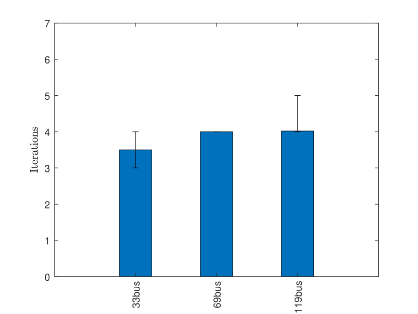
Figure 1: Average number of iterations to convergence of Algorithm III-B on the 33-node, 69-node, and 119-node IEEE distribution systems. The error bars show the maximum and minimum number of iterations to convergence for each test case.

Figure 2: Average number of iterations to convergence of Algorithm III-C on the 27 meshed cases from MATPOWER [8]. The error bars show the maximum and minimum number of iterations to convergence for each test case.

A similar observation is witnessed on the remaining test cases from PGLib-OPF [34]. Those remaining results are omitted here for ease of exposition but can be found in [47].

IV-C LMP and Q-LMP

The exactness of the solutions from Algorithm III-C also translates to accurate LMP and Q-LMP as shown in Table IV. Table IV also shows the maximum errors in nodal voltages and branch power flows. Table IV affirms that Algorithm III-C consistently produces accurate LMP and Q-LMP as well as accurate nodal voltages and branch power flows. This property entails that market operators already using LP solvers can not only generate more accurate LMP by using Algorithm III-C compared to the classical DC OPF, but can now offer a new avenue for pricing reactive power through Q-LMP, without changing their LP solvers.

TABLE IV: Algorithm III-C’s LMP, Q-LMP, node voltages, and branch power flows compared to those from KNITRO [9].

Test	Mean LMP	Mean Q-LMP	Max Voltage	Max $\bm{p_{ij}}$
Case	error ($\text{\,}\$\mathrm{/}\mathrm{M}\mathrm{VA}$)	error ($\text{\,}\$\mathrm{/}\mathrm{M}\mathrm{VAr}$)	error (pu)	error (pu)
5	7.44E-05	8.80E-04	9.40E-06	7.86E-06
6	8.06E-03	7.37E-03	4.10E-06	9.52E-04
9	2.29E-03	1.84E-04	3.73E-07	7.62E-05
14	1.20E-03	1.50E-03	1.85E-04	1.50E-04
24	2.37E-02	2.63E-02	6.28E-04	7.50E-04
IEEE30	1.20E-03	5.03E-04	1.70E-04	1.67E-04
30	5.15E-03	9.89E-03	1.57E-04	3.19E-04
39	3.44E-04	1.63E-03	3.32E-04	1.64E-04
57	9.58E-03	3.48E-02	2.06E-04	4.00E-04
89	1.15E-04	3.68E-05	3.75E-05	6.60E-03
118	2.31E-02	1.03E-02	8.32E-04	3.53E-03
200	7.51E-03	8.68E-04	1.08E-04	2.01E-03
300	1.66E-03	1.79E-03	1.34E-04	3.75E-04
1354	3.44E-05	2.52E-05	1.61E-04	5.48E-03
1888	2.76E-03	9.02E-03	1.53E-03	2.22E-02
1951	1.65E-05	6.84E-06	1.34E-03	5.98E-03
2383	6.63E-01	4.78E-01	4.38E-03	3.04E-03
2736	1.22E-02	2.04E-02	2.30E-04	1.35E-04
2737	4.12E-03	7.98E-03	2.08E-04	8.21E-05
2746wop	8.11E-03	6.92E-03	1.74E-04	4.77E-04
2746wp	5.77E-03	1.09E-02	1.67E-04	8.71E-05
2848	7.72E-05	1.15E-04	8.20E-04	2.27E-02
2868	2.92E-04	2.84E-04	1.03E-03	7.39E-03
2869	3.43E-05	2.29E-05	1.10E-04	3.58E-03
3012	9.25E-03	6.92E-03	1.41E-04	2.46E-04
3120	2.96E-02	1.83E-02	3.10E-04	3.59E-04
3375	7.36E-03	6.09E-03	7.96E-05	1.43E-04

Detailed LMP and Q-LMP profiles for the IEEE 57-bus test system obtained from KNITRO and Algorithm III-C are shown in Fig. 3.

\psfrag{Bus}{\footnotesize Bus \normalsize}\psfrag{LMP}{\footnotesize LMP $\left($\text{\,}\$\mathrm{/}\mathrm{M}\mathrm{W}$\right)$ \normalsize}\psfrag{AC OPF}{\footnotesize KNITRO \normalsize}\psfrag{Algorithm}{\footnotesize Algorithm~{}\ref{SLP_Meshed} \normalsize}\includegraphics[width=433.62pt]{./Figures/LMP57.eps}

() LMP.

\psfrag{Bus}{\footnotesize Bus \normalsize}\psfrag{QLMP}{\footnotesize Q-LMP $\left($\text{\,}\$\mathrm{/}\mathrm{M}\mathrm{VAr}$\right)$ \normalsize}\psfrag{AC OPF}{\footnotesize KNITRO \normalsize}\psfrag{Algorithm}{\footnotesize Algorithm~{}\ref{SLP_Meshed} \normalsize}\includegraphics[width=433.62pt]{./Figures/QLMP57.eps}

() Q-LMP.

Figure 3: LMP and Q-LMP of KNITRO [9] and Algorithm III-C on the IEEE 57-bus test system [8].

V Conclusion

This paper presented an SLP approach that exploits the structure of the alternative-form OPF by carefully constructing iteratively refined polyhedral outer approximations and supporting hyperplanes. Rigorous numerical evaluation on a wide range of test cases with up to 3375 buses shows that the method consistently converges to feasible high-quality solutions with robustness against the choice of starting point. While not claiming it is computationally superior to existing NLP solvers, the proposed method represents a competitive LP-based alternative, especially in settings where only LP solvers can be used or are practically deployed, e.g., market applications with shadow pricing of active and reactive power as well as congestion and losses. Another important benefit of the proposed SLP approach over NLP-based approaches is its potential straightforward extension to applications involving discrete decision variables, whereby powerful state-of-the-art MILP solvers can be used.

Appendix A Branch current limit constraints

In the polar-form OPF, the branch current magnitude is expressed as

$$i_{ij}=\sqrt{a_{1}v_{i}^{2}+a_{2}v_{j}^{2}-2v_{i}v_{j}\left(a_{3}\cos{\theta_{ij}}-a_{4}\sin{\theta_{ij}}\right)},$$ (A.1)

$$i_{ji}=\sqrt{a_{2}v_{i}^{2}+a_{1}v_{j}^{2}-2v_{i}v_{j}\left(a_{3}\cos{\theta_{ij}}+a_{4}\sin{\theta_{ij}}\right)},$$ (A.1)

where $a_{1}=\left(\tilde{g}^{\rm c^{*}}_{ij}\right)^{2}$, $a_{2}=\left(\tilde{g}^{*}_{ij}\right)^{2}$, $a_{3}=\Re\{\tilde{g}^{\rm c^{*}}_{ij}\}\Re\{\tilde{g}^{*}_{ij}\}+\Im\{\tilde{g}^{\rm c^{*}}_{ij}\}\Im\{\tilde{g}^{*}_{ij}\}$, and $a_{4}=\Re\{\tilde{g}^{\rm c^{*}}_{ij}\}\Im\{\tilde{g}^{*}_{ij}\}-\Im\{\tilde{g}^{\rm c^{*}}_{ij}\}\Re\{\tilde{g}^{*}_{ij}\}$. The limit constraint on the branch current magnitude can now be written as

$$i_{ij} \leq\overline{I}_{ij}, ij\in\mathcal{L}\cup\mathcal{L}_{\rm t},$$ (A.2)

where $\overline{I}_{ij}=\overline{I}_{ji}$ (pu) is the current rating of branch $ij$.

Constraints (A.1) are nonconvex and, as shown in [36], linearizing them is a daunting task. However, in the alternative-form OPF, those constraints can be replaced by linear equivalents. In more detail, by defining $\ell_{ij}:=i_{ij}^{2}$, and after substituting (1) in (A.1) and squaring both sides of the resulting equation, the branch current magnitude and associated limit become

$$\ell_{ij}=a_{1}w_{i}+a_{2}w_{j}-2a_{3}w_{ij}^{\rm r}+2a_{4}w_{ij}^{\rm i}, ij\in\mathcal{L}$$ , (A.3)

$$\ell_{ji}=a_{2}w_{i}+a_{1}w_{j}-2a_{3}w_{ij}^{\rm r}-2a_{4}w_{ij}^{\rm i}, ij\in\mathcal{L}$$ , (A.3)

$$\ell_{ij}\leq\overline{I}_{ij}^{2}. ij\in\mathcal{L}\cup\mathcal{L} {}_{\rm t}$$ (A.3)

The original current magnitude $i_{ij}$ can be straightforwardly obtained from the solution by taking the square root of $\ell_{ij}$ in a computationally cheap post-processing step.

Appendix B Proof of theorem 1

.

If $x^{(k)}$ minimizes $f_{0}(x)$ on $\mathcal{S}^{(k)}$ then it must satisfy the inequalities

$$f_{i}(x^{(\kappa)})+\nabla f_{i}(x^{(k)})^{T}(x^{(k)}-x^{(\kappa)})\leq 0,$$

$$\kappa=0,\ldots,k-1,\ i=1,\ldots,m.$$ (B.1)

Additionally, if $x^{(k)}$ contains a subsequence that converges to a point in $\mathcal{G}$ then every $f_{i}(x^{(k)}),i=1,\ldots,m\$ must contain a subsequence that converges to a value that is less than or equal to zero. If there exists a finite constant $K$ such that $\max\left(\left(\left\|\nabla f_{i}(x^{(k)})\right\|\right)_{i=1,\ldots,m}\right)\leq K$ for all $x\in\mathcal{S}^{(0)}$, and an $r>0$ independent of $k$, such that

$$\kappa=0,\ldots,k-1,\ i=1,\ldots,m,$$

then one can find a subsequence of iteration numbers where

$$\left\|x^{(u)}-x^{(v)}\right\|\leq r/K,\ \forall u<v,$$

so that $x^{(k)}$ does not contain a Cauchy sequence. However, because $\mathcal{S}^{(0)}$ is compact, no such $r$ exists, and $x^{(k)}$ therefore contains a subsequence that converges to a point $x^{\dagger}\in\mathcal{S}^{(0)}$. Finally, it follows from (B) that the corresponding subsequence of every $f_{i}(x^{(k)}),i=1,\ldots,m\$ converges to a value that is less than or equal to zero, which entails that $x^{\dagger}\in\mathcal{G}$ and $x^{\star}=x^{\dagger}$. ∎

Appendix C SLP example

Consider the nonconvex problem

whose optimal solution is $x^{*}=[x_{1}^{*},x_{2}^{*}]^{T}=[0,1]^{T}$. The novel SLP algorithm in this work solves the problem

at each iteration $k$ until convergence, measured by $\left|g\left(x^{(k)}\right)\right|\leq\epsilon$. A geometric interpretation of the SLP algorithm with $\rho=10$ and from starting point $x^{(0)}=[-2,2]^{T}$ is shown in Fig. 3() and Fig. 3() at $k=3$ and $k=7$, respectively.

() $k=3$.

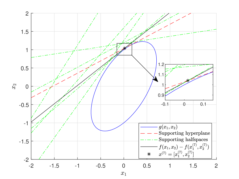
() $k=7$.

Figure 4: Geometric interpretation of the SLP algorithm at $k=3$ and $k=7$.

In Fig. 4, supporting hyperplanes (LABEL:example_slp_hyperp) are shown in red and supporting halfspaces (LABEL:example_slp_halfsp) are shown in green. The contour lines of $f\left(x\right)-f\left(x^{(k)}\right)$ and the nonconvex constraint $g\left(x\right)=0$ are shown in black and blue, respectively. The simultaneous inclusion of the supporting hyperplanes (LABEL:example_slp_hyperp) and the supporting halfspaces (LABEL:example_slp_halfsp) is essential for convergence. Without the hyperplanes in (LABEL:example_slp_hyperp) the algorithm converges to the solution of a convex relaxation of Problem C.1, i.e., one with $g\left(x\right)\leq 0$ instead of $g\left(x\right)=0$. Moreover, without the halfspaces in (LABEL:example_slp_halfsp) the algorithm fails to converge altogether. Furthermore, without the positive slack variable $r$ and the second term in (LABEL:example_slp_objective) some starting points, such as $x^{(0)}=[0,0]^{T}$ in this case, can lead to an infeasible LP Problem C.1. The robustness against the choice of starting point bestowed by $\rho r$ and (LABEL:example_slp_slack) is shown in Fig. 5 for $\epsilon=10^{-4}$, three choices of $\rho$, and 1000 starting points drawn from a uniform distribution in the interval $(-10,10)$ for both $x_{1}^{(0)}$ and $x_{2}^{(0)}$, i.e., $x_{1}^{(0)},x_{2}^{(0)}\sim\mathcal{U}\left(-10,10\right)$.

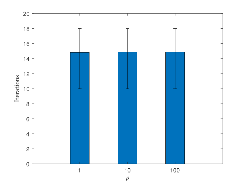
Figure 5: Average number of iterations to convergence of the proposed SLP algorithm initialized from 1000 different starting points for $\rho=1,10,100$. The error bars show the maximum and minimum number of iterations to convergence.

The error plot in Fig. 5 demonstrates a small variation in the number of iterations to convergence for $\rho=1,10,100$ over all the 1000 starting points, thus corroborating the robustness of the proposed SLP algorithm on Problem C.1.

More interestingly, the SLP algorithm applied to Problem C.1 converges much faster if the projection of point $x^{(k)}$ on the set defined by $g\left(x\right)=0$ is used instead of the first-order Taylor series approximation of $g\left(x\right)$ directly at $x^{(k)}$ (See Section III-A for more details on the projection).

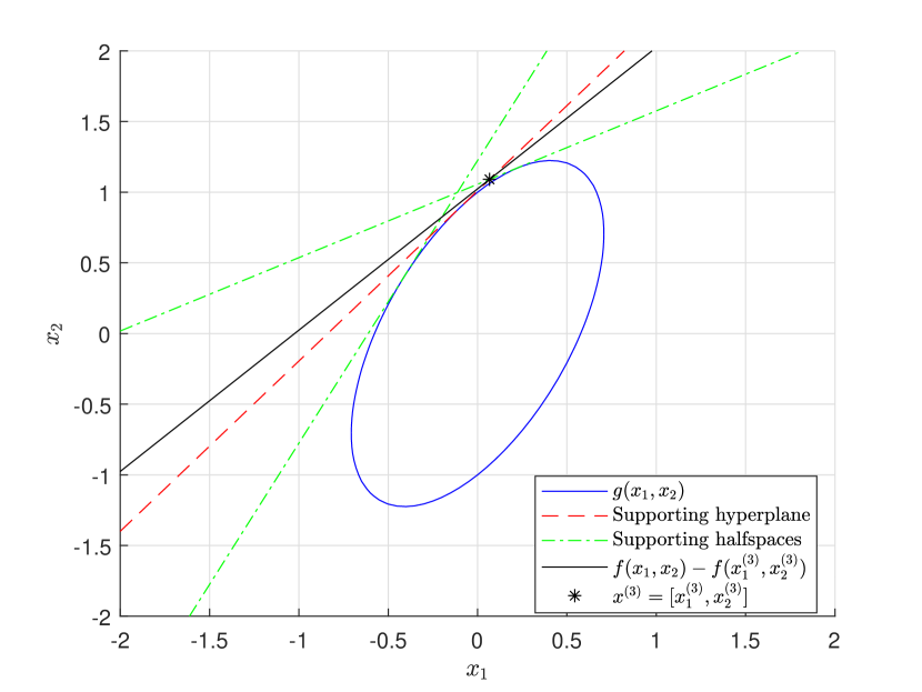
Figure 6: Geometric interpretation of the SLP algorithm with the projection of point $x^{(k)}$ on the set defined by $g\left(x\right)=0$ at $k=3$.

Fig. 6 shows that the modified SLP algorithm is already close to the optimal solution after only 3 iterations. In fact, as shown in Fig. 7, the proposed SLP algorithm with the projection of point $x^{(k)}$ on the set defined by $g\left(x\right)=0$ is on average $40\%$ faster compared to directly applying the first-order Taylor series approximation of $g\left(x\right)$ at $x^{(k)}$ (9 iterations on average for the modified SLP algorithm compared to 15 for the one with the first-order Taylor series approximation of $g\left(x\right)$ directly at $x^{(k)}$).

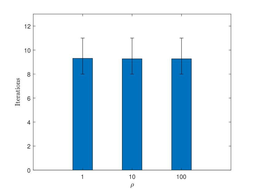
Figure 7: Average number of iterations to convergence of the proposed SLP algorithm with the projection of point $x^{(k)}$ on the set defined by $g\left(x\right)=0$. The algorithm is again initialized from 1000 different starting points for $\rho=1,10,100$. The error bars show the maximum and minimum number of iterations to convergence.

Finally, it is also evident form Fig. 4 and Fig. 6 that not all the supporting halfspaces are necessary for convergence. Some of the older inactive halfspaces can be removed for an improvement in computational speed.

Sleiman Mhanna (S’13–M’16) received the B.Eng. degree (with high distinction) from the Notre Dame University, Lebanon, and the M.Eng. degree from the American University of Beirut, Lebanon, in 2010 and 2012, respectively, both in electrical engineering. He received the Ph.D. degree from the School of Electrical and Information Engineering, Centre for Future Energy Networks, University of Sydney, Australia, in 2016. He is currently a Research Fellow at the Department of Electrical and Electronic Engineering, The University of Melbourne, Australia. His research interests include computational methods for integrated multi-energy systems, decomposition methods, and demand response.

Pierluigi Mancarella (SM) is Chair Professor of Electrical Power Systems at The University of Melbourne, Melbourne, Australia, and Professor of Smart Energy Systems at The University of Manchester, Manchester, UK. His research interests include techno-economic modeling of integrated multi-energy systems; security, reliability and resilience of future networks; and energy infrastructure planning under uncertainty. Pierluigi is an Editor of the IEEE Transactions on Power Systems, IEEE Transactions on Smart Grid, and IEEE Systems Journal, and an IEEE Power and Energy Society Distinguished Lecturer.

References

- [1] K. Lehmann, A. Grastien, and P. Van Hentenryck, “AC-Feasibility on Tree Networks is NP-Hard,” IEEE Transactions on Power Systems, vol. 31, no. 1, pp. 798–801, jan 2016.
- [2] D. Bienstock and A. Verma, “Strong NP-hardness of AC power flows feasibility,” Operations Research Letters, vol. 47, no. 6, pp. 494–501, dec 2019.
- [3] J. Carpentier, “Contribution à l’étude du dispatching économique,” Bulletin de la Société Française des Éléctriciens, vol. 3, August 1962.
- [4] J. A. Momoh, M. E. El-Hawary, and R. Adapa, “A Review of Selected Optimal Power Flow Literature to 1993 Part II: Newton, Linear Programming and Interior Point Methods,” IEEE Transaction on Power Systems, vol. 14, no. 1, pp. 105–111, 1999.
- [5] ——, “A Review of Selected Optimal Power Flow Literature to 1993 Part I: Nonlinear and Quadratic Programming Approaches,” IEEE Transactions on Power Systems, vol. 14, no. 1, pp. 96–104, 1999.
- [6] S. Frank, I. Steponavice, and S. Rebennack, “Optimal power flow: A bibliographic survey I Formulations and deterministic methods,” Energy Systems, vol. 3, no. 3, pp. 221–258, 2012.
- [7] F. Capitanescu, “Critical review of recent advances and further developments needed in AC optimal power flow,” pp. 57–68, 2016.
- [8] R. Zimmerman, C. Murillo-Sánchez, and R. Thomas, “MATPOWER: Steady-state operations, planning, and analysis tools for power systems research and education,” Power Systems, IEEE Transactions on, vol. 26, no. 1, pp. 12–19, Feb 2011.
- [9] R. H. Byrd, J. Nocedal, and R. A. Waltz, “Knitro: An integrated package for nonlinear optimization,” in Large Scale Nonlinear Optimization, 35–59, 2006. Springer Verlag, 2006, pp. 35–59.
- [10] A. Castillo, P. Lipka, J.-P. Watson, S. S. Oren, and R. P. O’Neill, “A successive linear programming approach to solving the IV-ACOPF,” IEEE Transactions on Power Systems, vol. 31, no. 4, pp. 2752–2763, 2016.
- [11] A. Gopalakrishnan, A. U. Raghunathan, D. Nikovski, and L. T. Biegler, “Global optimization of Optimal Power Flow using a branch & bound algorithm,” 2012 50th Annual Allerton Conference on Communication, Control, and Computing, Allerton 2012, pp. 609–616, 2012.
- [12] J. Liu, M. Bynum, A. Castillo, J. P. Watson, and C. D. Laird, “A multitree approach for global solution of ACOPF problems using piecewise outer approximations,” Computers and Chemical Engineering, vol. 114, pp. 145–157, 2018.
- [13] J. Kardos, D. Kourounis, O. Schenk, and R. Zimmerman, “Complete results for a numerical evaluation of interior point solvers for large-scale optimal power flow problems,” arXiv, 2018.
- [14] B. Stott and O. Alsaç, “Optimal power flow–basic requirements for real-life problems and their solutions (White paper),” SEPOPE XII Symposium, Rio de Janeiro, Brazil, pp. 1866–1876, 2012.
- [15] C. Coffrin, B. Knueven, J. Holzer, and M. Vuffray, “The Impacts of Convex Piecewise Linear Cost Formulations on AC Optimal Power Flow,” pp. 1–10, 2020. [Online]. Available: http://arxiv.org/abs/2005.14087
- [16] B. Stott, J. Jardim, and O. Alsaç, “DC power flow revisited,” IEEE Transactions on Power Systems, vol. 24, no. 3, pp. 1290–1300, 2009.
- [17] T. N. Dos Santos and A. L. Diniz, “A dynamic piecewise linear model for DC transmission losses in optimal scheduling problems,” IEEE Transactions on Power Systems, vol. 26, no. 2, pp. 508–519, 2011.
- [18] H. Zhong, Q. Xia, Y. Wang, and C. Kang, “Dynamic economic dispatch considering transmission losses using quadratically constrained quadratic program method,” IEEE Transactions on Power Systems, vol. 28, no. 3, pp. 2232–2241, 2013.
- [19] B. F. Hobbs, E. Bartholomew, Y. Chen, G. Drayton, and W. Lise, “Improved Transmission Representations in Oligopolistic Market Models: Quadratic Losses, Phase Shifters, and DC Lines,” IEEE Transaction on Power Systems, vol. 23, no. 3, pp. 1018–1029, 2008.
- [20] Z. Yang, H. Zhong, A. Bose, T. Zheng, Q. Xia, and C. Kang, “A Linearized OPF Model with Reactive Power and Voltage Magnitude: A Pathway to Improve the MW-Only DC OPF,” IEEE Transactions on Power Systems, vol. 33, no. 2, pp. 1734–1745, 2018.
- [21] K. Baker, “Solutions of DC OPF are Never AC Feasible,” arXiv, pp. 1–4, 2019. [Online]. Available: http://arxiv.org/abs/1912.00319
- [22] R. O’Neill, T. Dautel, and E. Krall, “Recent ISO software enhancements and future software and modeling plans,” FERC Staff Technical Paper, no. November, 2011.
- [23] W. Sauer, “Uplift in RTO and ISO Markets,” Federal Energy Regulatory Commission, Washington, DC, USA, Tech. Rep., 2014.
- [24] R. A. Jabr, “Radial distribution load flow using conic programming,” IEEE Transactions on Power Systems, vol. 21, no. 3, pp. 1458–1459, 2006.
- [25] A. G. Expósito and E. R. Ramos, “Reliable load flow technique for radial distribution networks,” IEEE Transactions on Power Systems, vol. 14, no. 3, pp. 1063–1069, aug 1999.
- [26] X. Bai, H. Wei, K. Fujisawa, and Y. Wang, “Semidefinite programming for optimal power flow problems,” International Journal of Electrical Power and Energy Systems, vol. 30, no. 6-7, pp. 383–392, 2008.
- [27] S. H. Low, “Convex relaxation of optimal power flow-part II: Exactness,” IEEE Transactions on Control of Network Systems, vol. 1, no. 2, pp. 177–189, 2014.
- [28] S. Huang, Q. Wu, J. Wang, and H. Zhao, “A Sufficient Condition on Convex Relaxation of AC Optimal Power Flow in Distribution Networks,” IEEE Transactions on Power Systems, vol. 32, no. 2, pp. 1359–1368, 2017.
- [29] F. Zohrizadeh, C. Josz, M. Jin, R. Madani, J. Lavaei, and S. Sojoudi, “A Survey on Conic Relaxations of Optimal Power Flow Problem,” 2019.
- [30] E. W. Cheney and A. A. Goldstein, “Newton’s method for convex programming and Tchebycheff approximation,” Numerische Mathematik, vol. 1, no. 1, pp. 253–268, 1959.
- [31] J. E. Kelley, Jr., “The Cutting-Plane Method for Solving Convex Programs,” Journal of the Society for Industrial and Applied Mathematics, vol. 8, no. 4, pp. 703–712, 1960.
- [32] L. P. Sampath, B. V. Patil, H. B. Gooi, J. M. Maciejowski, and K. V. Ling, “A trust-region based sequential linear programming approach for AC optimal power flow problems,” Electric Power Systems Research, vol. 165, no. April, pp. 134–143, 2018.
- [33] Z. Yang, H. Zhong, Q. Xia, A. Bose, and C. Kang, “Optimal power flow based on successive linear approximation of power flow equations,” IET Generation, Transmission and Distribution, vol. 10, no. 14, pp. 3654–3662, 2016.
- [34] S. Babaeinejadsarookolaee, A. Birchfield, R. D. Christie, C. Coffrin, C. DeMarco, R. Diao, M. Ferris, S. Fliscounakis, S. Greene, R. Huang, C. Josz, R. Korab, B. Lesieutre, J. Maeght, D. K. Molzahn, T. J. Overbye, P. Panciatici, B. Park, J. Snodgrass, and R. Zimmerman, “The Power Grid Library for Benchmarking AC Optimal Power Flow Algorithms,” arXiv, pp. 1–17, 2019.
- [35] R. P. O’Neill, A. Castillo, and M. B. Cain, “The IV formulation and linear approximations of the AC optimal power flow problem (OPF Paper 2),” FERC Staff Technical Paper, no. December, pp. 1–18, 2012.
- [36] D. Shchetinin, T. T. De Rubira, and G. Hug, “On the Construction of Linear Approximations of Line Flow Constraints for AC Optimal Power Flow,” IEEE Transactions on Power Systems, vol. 34, no. 2, pp. 1182–1192, 2019.
- [37] S. Mhanna, G. Verbič, and A. C. Chapman, “Tight LP Approximations for the Optimal Power Flow Problem,” 19th Power Systems Computation Conference, PSCC 2016, 2016.
- [38] “Gurobi Optimizer Reference Manual, Version 9.0,” pp. 1–786, 2019. [Online]. Available: www.gurobi.com
- [39] “IBM ILOG CPLEX. ver. 12.9.” [Online]. Available: http://www-01.ibm.com/software/integration/optimization/cplex-optimizer
- [40] M. E. Baran and F. F. Wu, “Network reconfiguration in distribution systems for loss reduction and load balancing,” IEEE Transactions on Power Delivery, vol. 9, no. 4, pp. 1401–1407, 1989.
- [41] R. Fletcher, S. Leyffer, and P. L. Toint, “On the Global Convergence of an SLP-Filter Algorithm,” Univ. Dundee, Aug. 1998, Numerical Analysis Report NA/183.
- [42] J. Bezanson, A. Edelman, S. Karpinski, and V. B. Shah, “Julia: A fresh approach to numerical computing,” SIAM review, vol. 59, no. 1, pp. 65–98, 2017.
- [43] I. Dunning, J. Huchette, and M. Lubin, “Jump: A modeling language for mathematical optimization,” SIAM Review, vol. 59, no. 2, pp. 295–320, 2017.
- [44] M. E. Baran and F. F. Wu, “Optimal capacitor placement on radial distribution systems,” IEEE Transactions on Power Delivery, vol. 4, no. 1, pp. 725–734, 1989.
- [45] Savier J. S. and D. Debapriya, “Impact of network reconfiguration on distribution systems performance,” IEEE Power Delivery, vol. 22, no. 4, pp. 2473–2480, 2007.
- [46] D. Zhang, Z. Fu, and L. Zhang, “An improved TS algorithm for loss-minimum reconfiguration in large-scale distribution systems,” Electric Power Systems Research, vol. 77, no. 5-6, pp. 685–694, 2007.
- [47] “SLP results.” [Online]. Available: https://drive.google.com/drive/folders/1qU81wlSvGu9QMknOuLtFV_gUfMUkaWPb?usp=sharing