Absolute Parameters of Young Stars: PU Pup

Abstract

We present combined photometric and spectroscopic analyses of the southern binary star PU Pup. High-resolution spectra of this system were taken at the University of Canterbury Mt. John Observatory in the years 2008 and again in 2014-15. We find the light contribution of the secondary component to be only $\sim$2% of the total light of the system in optical wavelengths, resulting in a single-lined spectroscopic binary. Recent TESS data revealed grazing eclipses within the light minima, though the tidal distortion, examined also from HIPPARCOS data, remains the predominating light curve effect. Our model shows PU Pup to have the more massive primary relatively close to filling its Roche lobe. PU Pup is thus approaching the rare ‘fast phase’ of interactive (Case B) evolution. Our adopted absolute parameters are as follows: $M_{1}$ = 4.10 ($\pm$0.20) M_⊙, $M_{2}$ = 0.65 ($\pm$0.05) M_⊙, $R_{1}$ = 6.60 ($\pm$0.30) R_⊙, $R_{2}$ = 0.90 ($\pm$0.10) R_⊙; $T_{1}$ = 11500 ($\pm$500) K, $T_{2}$ = 5000 ($\pm$350) K; photometric distance = 186 ($\pm$20) pc, age = 170 ($\pm$20) My. The less-massive secondary component is found to be significantly oversized and overluminous compared to standard Main Sequence models. We discuss this discrepancy referring to heating from the reflection effect.

1 Introduction

The system PU Puppis (= HR2944, HD61429, HIP 37173), also known as m Pup, is a relatively bright (B = 4.59, V = 4.70) early type giant (B8III, Garrison & Gray 1994) located at a distance of about 190 pc with the galactic co-ordinates $\lambda\sim$2407, $\beta\sim$ –18. Garrison & Gray (1994) noted its strong rotation, though without any significant effect apparent in its 4-colour photometric indices. While Jaschek et al. (1969) have given the spectral type of PU Pup to be B9V from its $UBV$ colour indices, Stock et al. (2002) determined the type to be B8IV from the system’s ($B-V)_{0}$.

The photometric variability was announced by Stift (1979) during a programme monitoring other stars in the sky region nearby. Stift noticed the variable had been reported as a component of the close visual double ADS 6246, the companion being of similar spectral type and magnitude, with a separation of about 0.1 or about 20 AU perpendicular to the line of sight. A corresponding period of the order of 30 years or greater for this wide pair might then be expected. Stift surmised that the close binary might be of the W UMa or $\beta$ Lyr kinds, but the relatively early type and long period would make PU Pup a very atypical representative of the first of these classes. The star appears to have received relatively little individual attention, but its variability was confirmed by the HIPPARCOS satellite (ESA 1997).

van den Bos (1927) first reported that m Pup was a close visual double and it appears as number 731 in his fourth list of new southern doubles, with the remark “too close”. The Washington Visual Double Star Catalogue 1996.0 (Worley & Douglas 1997) added the note “Duplicity still not certain. Needs speckle.” The latest (internet) edition of the Washington Double Star Catalogue mentions that the double star identification now seems likely to be spurious, as the system was unresolved by the high altitude SOAR telescope on 5 occasions between 2009 and 2013.

Stift (1979) gave the period of the variable to be 2.57895 d with the primary minimum epoch 2443100. This is significantly different from the period given by HIPPARCOS of 2.58232 days, at epoch 2448501.647, although the form of the light curve given by Stift appears essentially similar to that of HIPPARCOS. Stift (1979) considered other period possibilities, suggesting uncertainty in his evaluation, nevertheless the original period was retained in recent editions of the GCVS (Samus et al. 2017). The Eclipsing Variables catalogue of Svechnikov & Kuznetsova (1990) lists PU Pup as having a $\beta$ Lyr type light curve, composed of two near Main Sequence stars with the orbital inclination of about 70.5 deg, the relatively shallow minima being presumably offset by the light of the supposed third component, which would contribute about 45% of the photometrically monitored light, using the magnitude difference of van den Bos (1927). The two minima, at around 0.05 and 0.04 mag depth, appeared too shallow for the system to be regarded as eclipsing without third light; however, an ellipsoidal type variability may still fit the data if there is little or no third light. Budding et al. (2019) solved the HIPPARCOS light curve of PU Pup and proposed a relatively close binary star model with a rather low mass ratio and low inclination to give the ellipsoidal form of its light variation.

Recent high accuracy TESS monitoring (Ricker et al. 2014) of PU Pup showed that, although the predominating effect in the light curve is that of the tidal distortion (‘ellipticity effect’), grazing eclipses do occur at the base of the two minima per orbit, allowing a firm constraint on the orbital inclination.

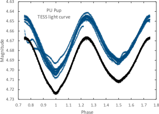
Figure 1: TESS light curves of PU Pup. The lower (black) points show the SAP data, while the upper (blue) points display the PDCSAP data from the MAST archive. The vertical axis gives the magnitude of the system, while the horizontal axis is the orbital phase as per equation 1

2 Orbital Period

Previous differences in the period values, mentioned in Section 1, prompted us to check this parameter. PU Pup (TIC 110606015) was observed by Transiting Exoplanet Survey Satellite (TESS) during Sector 7 of the mission, with two-minute cadencing. These light curves were downloaded from the Mikulski Archive for Space Telescopes (MAST) (cf. Jenkins et al. 2016). We used the straight Simple Aperture Photometry (SAP) data, since the Pre-search Data Conditioning Simple Aperture Photometry (PDCSAP) is optimized for planet transits and it appears that the PDCSAP detrending leads to additional effects in the 13.7 d period light curves of PU Pup (see Figure 1). After outliers (having non-zero ‘quality’ flags) were removed from the SAP data, about 17,000 points remained for analysis. With its high inherent accuracy (each datum is of the order of 0.0001 mag) the TESS light curves of PU Pup allowed us to discern small eclipse effects at the base of both light minima (see Figure 8). These effects would not have been noticeable in typical Earth-based photometry, or even that of HIPPARCOS. Fourier analysis of TESS light curves of the system was carried out using the program Period04 (Lenz & Breger 2005). As can be seen from Figure 2, only one dominant frequency was obtained as $f_{1}=0.77448\>(\pm\>0.00003)$ cycle/days. The period equivalent of this frequency is 1.29119 days, which corresponds to half of the orbital period; i.e. $P_{orb}=2.58237\>(\pm\>0.00005)$ d.

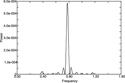
Figure 2: The Fourier spectrum of TESS data of PU Pup, plotting frequency on the horizontal axis and power on the vertical axis.

The TESS satellite observed 10 primary minima and 8 secondary minima of PU Pup over two observation cycles. The flux measurements were converted to magnitudes, and times of these minimum light were computed using a standard fortran program based on the K-W method (Kwee & van Woerden 1956; see also Ghedini 1982). These times of minima are given in Table A1 of the Appendix.

We sought to check on $O-C$ variations for a change in the orbital period. Although PU Pup is a relatively bright star, since the minimum depths of its light curves are very shallow, literature times of minima are few and sparsely arranged in time. We found only the KWS $V$ and $I$ data (from the Kamogata/Kiso/Kyoto Wide-Field Survey; Maehara 2014), apart from those of Stift (1979), HIPPARCOS and TESS mentioned already. We applied a method similar to the automated fitting procedure of Zasche et al. (2014) to derive individual times of minima of PU Pup from HIPPARCOS and KWS. The $O-C$ (observed minus calculated times of minima) values, listed in the Appendix, were examined from such findings. Our are plotted against the cycle number and observation years in Figure 3. The $O-C$ diagram of PU Pup shows a linear trend. Using a linear ephemeris model and least-squares optimization, the following result was obtained:

$$T_{min}=2448501.6306(11)+2.5822297(3)\times E.$$ (1)

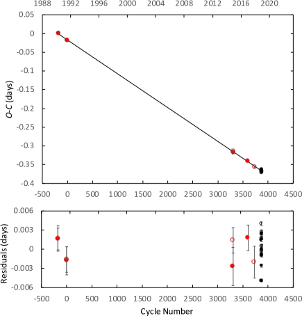
Figure 3: $O-C$ diagram of PU Pup: the $O-C$ values for times of minima (obtained directly from the TESS observations, are shown as black circles) while the $O-C$ values for times of minima (derived using the theoretical LC templates) are given as red circles. The $O-C$ values for the times of primary and secondary minima are also indicated by filled and hollow symbols respectively. The bottom panel shows the residuals from the linear model. Cycle number is the number of orbits from the starting epoch given in equation 1.

Comparing the mean period values from the epoch of Stift (1979) to the latest TESS times of minima (Table 1) there is a suggestion that the period is shortening. A typical estimate of $\Delta P/P$ is $\sim-3\times 10^{-8}$ per orbit or $-4\times 10^{-6}$ per year, over the last $\sim 40$ years. But the main result is that while we may derive an improved mean period and reference epoch, the data are too sparse for reliable period analysis. Although the $O-C$ diagram in Figure 3 does not give any clues to support the third light estimated from the light curve modeling (Section 4) or any changes in the orbital period of PU Pup, it is also noted that the scatter in the TESS data is larger than the expected timing accuracy ($\sim$ 5 minutes) suggestive of perhaps some short term irregularity.

Table 1: Mean Periods Over Longer Time Intervals. The Hipparcos epoch and period is used for reference. ‘TOM’ stands for Time of Minimum, $P$ the orbital period, and $\Delta P/P$ the linear change in period per orbit.

Epoch	ToM	Orbits	Mean $P$	$\Delta P/P$
HJD240000+
43099.4336	43100.00	-2092	2.5820492	$-1.29\times 10^{-7}$
54805.0901	54804.8319	2441	2.5822142	$-4.33\times 10^{-8}$
56669.5252	56669.2096	3163	2.5822202	$-3.15\times 10^{-8}$

3 Spectroscopy

Spectroscopic data on PU Pup have been collected using the High Efficiency and Resolution Canterbury University Large Échelle Spectrograph (HERCULES) of the Department of Physics and Astronomy, University of Canterbury, New Zealand (Hearnshaw et al. 2002) on the 1 m McLellan telescope of the Mt John University Observatory (MJUO) near Lake Tekapo ($\sim$4359’ S, $\sim$17427’ E). A few dozen high-dispersion spectra have been taken of the system over the last decade. A reasonable phase coverage of the system’s radial velocity variations was first collected in 2008.

To attain a fair signal to noise (S/N) ratio (typically around 100) the 100 micron optical diameter fibre cable has generally been used. This enables a theoretical resolution of $\sim 40,000$. Typical exposure times were about 500 seconds for the SI600s CCD camera. The raw data were reduced with HRSP 5.0 and 7.0 (Skuljan 2014, 2020), the échelle’s spectral orders between 85 and 125 being convenient for stellar spectral image work. We applied IRAF tools to the HRSP-produced image files in order to determine information such as the radial and rotational velocities. The IRAF routine SPLOT was useful in this context.

Spectral orders and lines used for line identifications and RV measurements are given in Table 2. The plots of spectral orders selected from the spectrum of PU Pup taken on the night of December 03, 2015 and at the conjunction phase are also shown in Figure B-1 in Appendix B as an example. Non-hydrogen lines that could be measured well (Table 2: the He I lines and the Si II $\lambda$5056 feature) have a depth of typically $\sim$3% of the continuum. Such lines are relatively wide, with a width at base of typically $\sim$6 Å or $\sim$220 pixels. The hydrogen lines are, of course, much better defined, but they are very broadened and perhaps complicated by dynamical effects in the system or over component surfaces. The positioning of a well-formed symmetrical (non-H) line can be expected to be typically achieved to within $\sim$10 pixels or (equivalently) up to $\sim$10 km/s. The measured lines move in accordance with only one spectrum, the system is thus ‘single lined’ and no feature unequivocally from the secondary could be definitely identified.

The equivalent width (ew) of H$\beta$ was measured to be typically $\sim$7.5, and that of He I 6678 to be $\sim$0.12. While the He I ew points to a spectral type of about B8, the corresponding ew value for H$\beta$ would be higher for a normal dwarf at B8. The issue is resolved by the lower gravity luminosity classifications of Garrison & Gray (1994) and Stock et al. (2002).

Table 2: Spectral Line Identifications. Asterisks refer to the appearance of the same line on successive orders.

Species	Order no.	$\lambda$	Comment
He I	85	6678.149	strong
H$\alpha$	87	6562.81	not used for rv
Si II	89	6371.359	moderate
Si II	90	6347.10	moderate
He I	97	5875.65	strong
Fe II	107	5316.609	moderate
Fe II	110	5169.03	moderate
Si II	112	5056.18	strong∗
Si II	113	5056.18	strong∗
H$\beta$	117	4861.3	not used for rv
Fe II	124	4583.829	weak
Fe II	125	4549.50	Fe II + Ti II blend

3.1 Radial Velocities

Mean wavelengths were derived using the IRAF SPLOT tool (k-k) on the strong lines in Table 2 as taken from MJUO observations made in 2008, 2014 and 2015. These produced the representative radial velocities (RVs) given in Table 3. The listed dates and velocities have been corrected to heliocentric values with the aid of the HRSP and IRAF program suites.

Table 3: Radial Velocity Data for PU Pup. Error estimates, typically of order 5 km s^-1 for individual measures, are indicated in Figure 4, and discussed in the text.

No	HJD	Phase	RV	No	HJD	Phase	RV
	245+		km s-1		245+		km s-1
1	4802.9063	0.154	-9.0	1	6667.0814	0.053	1.4
2	4803.0954	0.228	1.9	2	6668.0849	0.442	41.1
3	4803.1365	0.243	7.5	3	6668.8805	0.750	52.3
4	4803.9004	0.539	47.4	4	6668.9080	0.761	52.9
5	4803.9124	0.544	54.3	5	6668.9366	0.772	52.0
6	4803.9554	0.560	56.2	6	6669.8787	0.137	1.4
7	4804.9119	0.931	26.3	7	6669.8871	0.140	-0.5
8	4804.9812	0.958	14.8	8	6669.9238	0.154	0.1
9	4805.0601	0.988	13.1	9	6670.0036	0.185	0.9
10	4805.0946	0.002	22.3	10	6670.8790	0.524	52.0
11	4805.1247	0.013	7.7	11	6670.9174	0.539	57.2
12	4805.1478	0.022	6.0	12	6671.0332	0.584	59.8
13	4806.9436	0.718	56.9	13	6671.8804	0.912	23.2
14	4806.9594	0.724	58.0	14	6674.8775	0.073	2.1
15	4807.0531	0.760	53.8	15	6675.9159	0.475	46.5
16	4807.0595	0.762	58.3	16	6675.9567	0.490	47.6
17	4807.1052	0.780	51.7	1	7354.0749	0.091	2.3
18	4807.1101	0.782	51.7	2	7356.0368	0.851	35.5
19	4807.1157	0.784	52.0	3	7356.9445	0.202	5.6
				4	7357.9875	0.606	57.5
				5	7360.0906	0.421	41.0
				6	7360.9733	0.762	51.7

The RVs from Table 3 were fitted with an optimized binary system model using the program fitrv4a. The results are shown in Figure 4, and the corresponding parameters listed in Table 4.

The korel program (Hadrava 2004) was also used to check the RV measurements in Table 3 and spectroscopic orbital solutions in Table 4 and to increase their reliability. For this, the prominent H$\beta$ lines were chosen. The spectra of the secondary component were not disentangled, it being assumed that – in this particular case of such a relatively low luminosity companion – H$\beta$ is effectively unblended. The korel fits and line profiles of the H$\beta$ line are shown in Figure 5.

The mean epoch of the 2008 RV curve is HJD 2454805.0901. We may note from Figure 4 (upper panel) that the epoch of zero phase on the rv curve has occurred before the ephemeris-predicted zero phase by an interval of 0.0883. In other words, there has developed an ‘$O-C$’ of $-0.228$ days over the 2,441 orbital cycles after the HIPPARCOS zero phase epoch. This implies a noticeable rate of secular period decrease of order $\Delta P/P\sim 3\times 10^{-8}$. If a similar calculation is made for the 2014 — 2015 radial velocity solutions as given in Table 4, a period decrease of the same order is found.

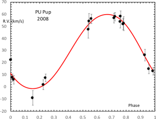
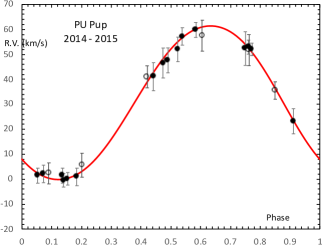
Figure 4: Our best-fitting binary RV curves for PU Pup: 2008 data (upper panel), and 2014 & 2015 data (lower panel). Hollow circles show 2014 data, while empty circles display 2015 data. The red lines represent the best fitting models. Orbital phase is given as the horizontal axis, and radial velocities in km/s on the vertical axis.

Figure 5: korel plot of H$\beta$ lines, from the 2008 data-set (upper panel), and 2014 & 2015 data-sets (lower panel) showing orbital motion.

Table 4: Binary Model RV Parameters for PU Pup. $K_{1}$ is the amplitude, $\phi_{0}$ the phase offset, and $V_{\gamma}$ the mean system velocity in km/s. $f(M)$ is defined by equation 2.

Parameter	2008	2014 – 2015
$K_{1}$ (km/s)	$31.5(\pm 1.3)$	$31.4(\pm 0.5)$
$\phi_{0}$ (deg)	$-31.8(\pm 2.5)$	$-44(\pm 1)$
$V_{\gamma}$	$29.3(\pm 1.0)$	$30.6(\pm 0.4)$
$a_{1}{\sin}i$ (R⊙)	1.61 (${\pm}$0.07)	1.60 (${\pm}$0.02)
$f(M)$ (M⊙)	0.0084 (${\pm}$0.0010)	0.0083 (${\pm}$0.0004)

Utilizing the mass function formula (Torres et al. 2010):

$$f(M)=C(1-e^{2})^{3/2}K_{1}^{3}P,$$ (2)

(where the constant $C=1.03615\times 10^{-7}$ when $K_{1}$ is in km s^-1 and $P$ is in days) gives $f(M)=0.0083$. This can be written as:

$$\frac{q^{3}}{(1+q)^{2}}=\frac{f(M)}{M_{1}\sin^{3}i}.$$ (3)

With the photometric value of $\sin i$ as 0.866 and a plausible estimate for $M_{1}$ as 4 $M_{\odot}$, we derive $q=0.16$, consistent with Table 6, as mentioned above. This leads to the secondary being a late K type dwarf with $V$-magnitude less than 1% that of the primary and thus not detectable spectroscopically. The separation of the components, using Kepler’s 3rd law, turns out to be about 13.2 $R_{\odot}$, so the rotational velocity of the primary, if synchronized, would be $\sim$124 km s^-1. With the derived inclination, a measured rotation speed of about 107 km s^-1 would then be expected.

3.2 Rotational Velocities

We fitted selected helium line profiles of PU Pup at various orbital phases using the program prof (Budding & Zeilik 1995; Budding et al. 2009). prof convolves Gaussian and rotational broadening, and can characterize the line profile in terms of the following adjustable parameters: continuum intensity $I_{c}$, relative depth $I_{d}$ at mean wavelength $\lambda_{m}$, rotational broadening parameter $r$ and Gaussian broadening parameter $s$ for a given line, and a limb-darkening coefficient $u$. Typical results of the profile fitting are shown in Figure 6 and given in Table 5.

Table 5: Profile Fitting Parameters For The He I 6678 Feature. See section 3.2 for an explanation of the symbols.

Parameter	Value	Error
Phase 0.21
$I_{c}$	1.001	0.008
$I_{d}$	0.027	0.007
$\lambda_{m}$	6679.547	0.045
$r$	2.31	0.20
$s$	0.33	0.06
$\chi^{2}/\nu$, $\Delta l$	1.23	0.01
Phase 0.73
$I_{c}$	0.999	0.008
$I_{d}$	0.025	0.010
$\lambda_{m}$	6680.962	0.043
$r$	2.27	0.22
$s$	0.22	0.08
$\chi^{2}/\nu$, $\Delta l$	1.26	0.01

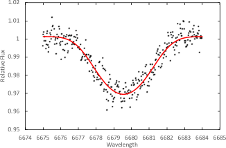
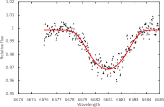
Figure 6: Results of profile fitting to the He I 6678 lines at elongation phases (top panel for phase 0.21 and bottom panel for phase 0.73). To show orbital motion and the line shift, the $x$-axis values are taken the same in both panels. Wavelength is plotted on the horizontal axis, and relative flux on the vertical.

According to the value of $r$ (the rotational broadening parameter) in Table 5, the mean observed projected rotational velocity of the primary component is $102\>({\pm}\>20)$ km/s. Using absolute parameters and assuming synchronous rotation, the theoretical projected rotational velocity for the primary component was found to be $107\>({\pm}\>10)$ km/s, so synchronous rotation can be accepted within the assigned error limits. The value of the Gaussian broadening $s$ changes between 25 and 15 km/s for the primary component according to the orbital phase. These values could be related to thermal broadening (with calculated thermal velocities in the order of $\sim$8 km/s), together with turbulence effects on the fairly distorted surface of the primary star.

4 TESS Photometry

Light curve analysis of the TESS data has been carried out using WinFitter program and the numerical integration code of Wilson & Devinney (1971) combined with the Monte Carlo (wd+mc) optimization procedure discussed by Zola et al. (2004). This second method allows modelling the binned TESS light curve of PU Pup by means of surface equipotentials, with suitable coefficients for gravity and reflection effect parametrization. In this wd+mc method, a range of variation, fixed by physically feasible limits, is set for each adjustable parameter. These ranges were selected in cognizance of the WinFitter modelling. The WD + MC program follows a search method involving the solution space consisting of tens of thousands of solutions in the given variation range of each adjustable parameter. Therefore, in the range of variation given in the manuscript, the WD + MC program performs mass and inclination searches (q-search and i-search.)

WinFitter has been applied in a number of recent similar studies to the present one. Its fitting function derives from Kopal (1959)’s treatment of close binary proximity effects, including tidal distortions of stellar envelopes of finite mass, and luminous interaction factors from the theoretical reflection-effect formulae of Hosokawa (1958). The main geometric parameters determined from the optimal fitting of light-curve data with this model are the orbital inclination $i$ and the mean radii ($r_{1,2}$) given in terms of the mean separation of the two components, corresponding to equivalent single stars. The latest version of WinFitter is available from Rhodes (2020).

The phases of the TESS photometric observations were computed using our derived new ephemeris, given as Equation 1 in Section 2. This was constructed from analysis of PU Pup’s times of minimum light, mentioned above. The phased TESS data were binned with between 100 and 150 individual points per phase bin, allowing more binned points at the eclipse phases. In this way, 128 points together with their uncertainties were used in the analysis. The uncertainties were derived from the published measurement information in the source data.

Regarding the orbital inclination, we used the following basic formula:

$$\delta^{2}=cos^{2}i +sin^{2}i\ sin^{2}\phi,$$ (4)

where $\delta$ is the separation of the two component star centres projected onto the celestial sphere, and $\phi$ is the orbital phase-angle and calculated from the primary mid-eclipse $T_{0}$ at time $T$ as $\phi=2\pi(T-T_{0})/P$. The term ‘grazing’ means a very small, slight eclipse when the phase  $\phi$ $\sim 0$. Then $cos\ i\approx\delta$. Considering $\delta\approx r_{1}+r_{2}$ and taking $r_{1}+r_{2}\gtrsim 0.5$ from the preliminary curve-fits of Budding et al. (2019), we find that the orbital inclination $i$ should be not far from 60^∘. Thus, inclination limits were set as $30^{\circ}<i<70^{\circ}$. The input range of the zero phase shift was taken as $-0.01<\Delta\phi_{0}<0.01$. The effective temperature ($T_{e}$) of the primary component of PU Pup was estimated from its spectral type (see Section 1). A compromise value of 11500 ($\pm\>500$) K was adopted. In a similar way, a mass for the primary was tentatively estimated as 4 M_⊙. Using the relationship between mass function and mass ratio (Section 3.1, Equation 3), the feasible input range of mass ratio ($q=M_{2}/M_{1}$) narrows to the range 0.15 — 0.18. This implies a mid-K type MS dwarf for the secondary with an effective temperature $T_{e}$ of around 5000 K. Since spectral features of the secondary component are not visible (see Section 3) and the photometric contribution of the secondary is small (Table 6), a direct confirmation of its properties is not practicable.

The available range for the non-dimensional surface potential parameters $\Omega_{1}$ and $\Omega_{2}$ was set as the range 1.0 — 8.0. The bolometric gravity effect exponent ($\beta_{1}$) and albedo ($A_{1}$) were taken as empirical adjustables, noting that the effect of the ellipsoidal form of primary component predominates. Given that the primary component has a radiative envelope, the input range for $\beta_{1}$ was set as 0.5 — 2. A range from 0.5 to 0.995 was allowed for the primary’s fractional luminosity ($L_{1}$). A quadratic limb-darkening law was used with limb-darkening coefficients taken from Claret (2017), where the effective wavelength of the broad TESS filter transmission function is derived for given $T_{e}$ values. In the present case this is not far from 800 nm. It was assumed that the components of PU Pup are rotating synchronously in a circular orbit. On the other hand, an $i$-search was performed for the values of orbital inclination between 50 and 70 degrees and a $q$-search for the values of the mass ratio between 0.10 and 0.30, using the DC code of the WD method. Fig. 7 shows the weighted sum of squared residuals for ranges in the orbital inclination and mass ratio, $\sum W(O-C)^{2}$, with $O$ being the observed data and $C$ the calculated points. As can be seen from these figure, the variation of the weighted sum of the squared residuals versus orbital inclination and mass ratio give a minimum around $i=60^{\circ}$ and $q=0.17$, respectively. The values of $i=61^{\circ}$ and $q=0.16$ obtained in the final model match these minimum values.

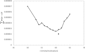
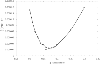
Figure 7: Behavior of the weighted sum of the squared residuals, $\sum W(O-C)^{2}$, as a function of orbital inclination $i$ (top panel) and mass ratio $q$ (bottom panel). The values of $i=61^{\circ}$ and $q=0.16$ of the final model are also shown as filled circles.

The final parameters for the best-fitting wd+mc model light curve of PU Pup are given in Table 6. The uncertainties of the adjustables are given as output from the wd+mc program and correspond, formally, to a 90$\%$ confidence level (Zola et al. 2004). $\chi^{2}$ was calculated as $\sum_{i}(\emph{l}_{i,o}-\emph{l}_{i,c})^{2}$/$\Delta\emph{l}_{i}^{2}$ from Bevington (1969), where $l_{i,o}$ and $l_{i,c}$ are the observed and calculated light levels at a given phase, respectively, and $\Delta\emph{l}_{i}$ is an error estimate for the measured values of $l_{i,o}$, taken to be 0.0002 in the relative flux. The reduced $\chi$-squared is given as $\chi^{2}_{red}$=$\chi^{2}/\nu$, where $\nu$ is the number of degrees of freedom of the data set (Bevington 1969). The adopted best-fit wd+mc light curve for the TESS photometry is shown in Figure 8. A three-dimensional projected illustration, including the grazing eclipses, obtained with BinaryMaker (Bradstreet & Steelman 2002), is displayed in Figure 9.

The wd+mc curve-fittings are compared with those of WinFitter (wf6) in Table 6. It can be seen directly that there is a fair measure of agreement in the main geometric parameters. The fittings call for some degree of third light ($L_{3}$). This related to how well the scale of the main ellipticity effect is controlled by the assigned parameters. This includes the proximity effect coefficients that depend on the given wavelength and temperatures. In the present context it is the primary’s tidal distortion, related to $\beta_{1}$ ($\tau_{1}$), and perhaps the secondary’s ‘reflection effect’, depending on $A_{2}$ ($E_{2}$), that can be influential.

It is appropriate to say more about these coefficients and their effects on the fittings. The $\beta$ parameters (wd+mc)represent the bolometric index of the gravity darkening, i.e. $H/H_{0}=(g/g_{0})^{\beta}$, where $H$ and $H_{0}$ are the local and mean surface radiative fluxes; $g$ and $g_{0}$ are the corresponding local and mean surface gravities. The $\tau$s are the corresponding coefficients in wf6. They represent the same indices, but corrected for the effect of wavelength and temperature of observation: an operation performed internally in both codes. It can be seen from Table 4-5 in Kopal’s (1959) book that these corrections reduce the role of the coefficient at higher temperatures and longer wavelengths. But both primary gravity coefficients $\beta_{1}$ and $\tau_{1}$ resulting from optimal curve-fitting to the TESS photometry are in keeping with, or somewhat greater than, the standard von Zeipel value of $\beta_{1}=1$ for a radiative envelope. The corresponding conversions for the reflection coefficient $A_{2}$ or $E_{2}$ (sometimes called geometric albedo) enhance the coefficient over its bolometric value at the low temperature of the secondary, but the low relative size of the secondary implies an essentially low scale of light reflection in PU Pup.

The difference in the zero phase correction $\Delta\phi_{0}$ arises from the use of different ephemerides: wf6 has used the period provided by the HIPPARCOS Epoch Photometry Catalogue (ESA 1997) together with a preliminary time of minimum taken to correspond with the lowest value of the TESS fluxes. wd+mc used the new ephemerides presented in the previous section.

The difference in the limb-darkening coefficients ($x_{i}$ and $y_{i}$ in Table 6) arise mainly from a slight but significant difference in the formulation between that of Claret (2017), used in wd+mc, and Kopal (1959 – ch. 4), used in wf6. The second-order limb-darkening effects ($y$s) were fixed at low values in the wf6 model, but it should be noted that in empirical curve-fitting there would be a linear correlation between the first and second-order coefficients that compromises their separate determinability. The selection of the limb-darkening approximation would have more significance for PU Pup if the eclipses were more prominent.

Table 6: The Results of Optimal Curve-fitting to the TESS Photometry of PU Pup using wd+mc and wf6 Photometry Modelling Programs. There is reasonable agreement between these different fitting codes that the inclination is close to 60^∘; the primary relative radius is $\sim$0.5 (and therefore the primary is not far from contact with its Roche Lobe), and the primary star is about 6 times larger in radius than its companion. The secondary is involved in the very shallow eclipses ($\sim$0.5% of the system light in depth), but other than that, its effects are weak. More details are given in the text.

Parameter	wd+mc	wf6	Error estimate
$T_{1}$ (K)	11500	11500	500
$T_{2}$ (K)	5560	5000	350
$q=M_{2}/M_{1}$	0.16	0.16	0.01
$L_{1}$	0.85	0.90	0.04
$L_{2}$	0.02	0.01	0.005
$L_{3}$	0.13	0.10	0.03
$\Omega_{1}$	2.303	—	0.03
$\Omega_{2}$	4.282	—	0.41
$r_{1}$ (mean)	0.49	0.51	0.02
$r_{2}$ (mean)	0.06	0.07	0.01
$i$ (deg)	61.0	56.2	1.1
$\Delta\phi$ (deg)	0.00	2.25	0.06
$\beta_{1}$ / $\tau_{1}$	1.30	0.49	0.23
$\beta_{2}$ / $\tau_{2}$	0.32	0.92	—
$A_{1}$ / $E_{1}$	0.51	0.17	0.12
$A_{2}$ / $E_{2}$	0.50	1.9	—
$x_{1}$	0.124	0.29	—
$x_{2}$	0.378	0.60	—
$y_{1}$	0.260	–0.02	—
$y_{2}$	0.213	–0.03	—
$\Delta l$	0.0002	0.0002	—
$\chi^{2}/\nu$	1.09	1.2	—

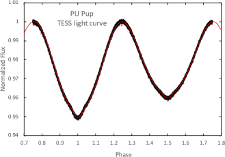
Figure 8: TESS light curve of PU Pup (the points) and wd+mc model (the red line) fitting. Normalized flux is plotted on the vertical axis, where the total flux of the system is set to unity. Orbital phase is plotted on the horizontal axis, starting at 0.7 and going to 1.8.

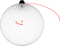
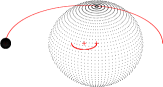
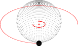
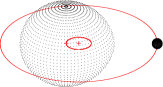
Figure 9: 3D model of PU Pup at conjunction (left bottom panel at phase 0.0 and left top panel at phase 0.5) and elongation (right bottom panel at phase 0.25 and right top panel at phase 0.75).

5 Absolute Parameters

In the well-known ‘eclipse method’ photometric and spectroscopic findings are combined, making use of Kepler’s third law, to derive absolute stellar parameters. If the photometric mass ratio and orbital inclination in Table 6 are used in Eqn 3, the mass of the primary component is found to be $M_{1}$ = 4.10 ($\pm\>0.20$) M_⊙. The mass of the secondary component, $M_{2}\approx 0.65$ M_⊙, then follows. The average distance between components, $A$, is calculated from Kepler’s third law. The fractional radii of components, $r_{1,2}$, obtained from the photometric curve-fits, lead to the listed absolute radii, $R_{1,2}$. Surface gravities ($g$) are then directly derived. Determination of the bolometric magnitude ($M_{bol}$) and luminosity ($L$) of the component stars requires the effective temperatures that were taken from Table 6. In the calculations, effective temperature T_e = 5771.8 ($\pm$0.7) K, M_bol = 4.7554 ($\pm$0.0004) mag, BC = –0.107 ($\pm$0.020) mag, and g = 27423.2 ($\pm$7.9) cm/s² were used for solar values (Pecaut & Mamajek 2013).

The absolute visual magnitude, M_V, involves the bolometric correction formula, $BC$ = $M_{bol}$ – $M_{V}$. Bolometric corrections for the components were taken from the tabulation of Flower (1996), according to the assigned effective temperatures. The photometric distance is calculated using the formula, $M_{V}$ = $m_{V}$ + 5 – 5log$(d)$ – $A_{V}$. For this, the interstellar absorption and intrinsic color index were computed using the method given by Tunçel Güçtekin et al. (2016). Firstly, the total absorption towards PU Pup in the galactic disk in the $V$ band, $A_{\infty}(V)$, was taken from Schlafly & Finkbeiner (2011), using the NASA Extragalactic Database. Then the interstellar absorption for PU Pup’s distance, $A_{d}(V)$, was derived from the formula given by Bahcall (1980) (their Eqn. 8), using the Gaia DR2 parallax (Gaia Collaboration 2018). The color excess for the system at this distance, $d$, was estimated as $E_{d}(B-V)$ = $A_{d}(V)$/3.1. Thus, the intrinsic color index of PU Pup was calculated as ($B-V$)₀ = –0.13 mag. This photometric distance – correcting for interstellar absorption – is then found to be 186 ($\pm$20) pc.

Our absolute parameters for the PU Pup system are given in Table 7 with their standard errors. By comparison, previous photometric parallax calculations (Popper 1998; Budding & Demircan 2007) result in a distance of 190 ($\pm$22) pc. The astrometric parallaxes of Gaia DR2 (Gaia Collaboration 2018) and HIPPARCOS (van Leeuwen 2007) produce distances of 176 ($\pm$10) and 190 ($\pm$10) pc, respectively. This consistency between the distances calculated by different methods, taking into account their standard errors, allows confidence in the observationally determined absolute parameters of PU Pup in the present study.

Table 7: Absolute Parameters of PU Pup. Certain priors in this table were adopted from published sources thus: ^a Fabricius et al. (2002), ^b Gaia Collaboration (2018), and ^c van Leeuwen (2007). Terms are as defined in the text.

Parameter	Primary	Secondary
$A$ (R⊙)	13.30 ($\pm$0.40)
$M$ (M⊙)	4.10 ($\pm$0.20)	0.65 ($\pm$0.05)
$R$ (R⊙)	6.60( $\pm$0.30)	0.90 ($\pm$0.10)
log $g$ ($cm/s^{2}$)	3.40 ($\pm$0.05)	4.30 ($\pm$0.10)
$T$ (K)	11500 ($\pm$500)	5000 ($\pm$350)
$L$ (L⊙)	695 ($\pm$80)	0.50 ($\pm$0.10)
$M_{bol}$ (mag)	–2.35 ($\pm$0.20)	5.54 ($\pm$0.40)
$M_{V}$ (mag)	–1.77 ($\pm$0.22)	5.85 ($\pm$0.45)
$E$($B-V$) (mag)	0.041
$B-V$ (mag)	–0.09a
$V$ (mag)	4.67a
$M_{V}$ $(system)$ (mag)	–1.80 ($\pm$0.25)
$d$ (pc)	186 ($\pm$20)
$d_{Gaia-DR2}$(pc)	176 ($\pm$10)b
$d_{HIP}$(pc)	190 ($\pm$10)c

6 Evolutionary Status

The ellipticity effect predominantly from the primary component and small (grazing) eclipses give the ratio of radii of components as 0.15 in the light curve solutions. In other words, the radius of primary component is approximately 7 times larger than that of secondary component, and, as indicated by the low value of $\Omega_{1}$ in Table 6, this star is relatively close to filling its Roche Lobe. That is, the primary and secondary components fill 93% and 50% of their Roche lobes. This unusual configuration raises a challenge in piecing together the age and evolution of the system.

The Padova evolution models (Marigo 2017) display theoretical (mass – radius) and (mass – $T_{e}$) isochrone locations in Figure 10 corresponding to a metallicity of Z = 0.014. The primary appears to be close to the Terminal Age of the Main Sequence for its mass, with an age of about 170 My for Z = 0.014. However, it may be noted that this evolution model predicts a smaller radius and lower surface temperature than is observed for the secondary star.

A sensitive way to estimate Z from theoretical stellar models is from the log ($T_{e}$) – log ($g$) diagram. Looking at this in Figure 11, we deduce that the metallicity and age of the primary star are about Z = 0.014 ($\pm 0.003$) and 170 ($\pm 20$) Myr. We show only the primary in this diagram since the secondary is discordant for reasons that we consider below. Other predictions (e.g. from the BaSTI and Geneva stellar evolution models) were investigated and similar results were found.

With regard to the apparent luminosity excess of the secondary, this kind of problem is not uncommon in short-period binary systems (e.g., Garrido et al. 2019). Such inflated radii for relatively low mass components have been discussed in terms of fast rotation and tidal effects (e.g., Chabrier et al. 2007; Kraus et al. 2011). We should also keep in mind that the luminosity of the primary is greater than that of the secondary by about three orders of magnitude.

Padova models for a star of 0.65 M_⊙ with a typical young star metallicity (Z = 0.014-19) give a radius of $\sim$0.6 R_⊙ at the estimated age of around 170 My. These models show that even at $\sim$170 My, the low mass star is still condensing towards the Zero Age Main Sequence, but the increased luminosity from this would account for less than 1% of an increase in radius, i.e. insufficient to explain the $\sim$30% increase in radius over a standard model for an unevolved star of the secondary’s mass. A rough estimate shows the amount of radiated energy intercepted by the dwarf from the subgiant to be $\sim$10 times its own inherent luminosity. Assuming that the mean effective temperature of the secondary would increase by $\sim$20% with this energy input, the radius should double, in order to radiate away the excess energy and remain in thermal equilibrium. Of course, some of the flux received at the secondary may be simply scattered or else drive kinetic mass motions in the dwarf’s envelope, but in any case a significant increase in radius of the secondary can be reasonably anticipated on the basis of the heat received from the primary.

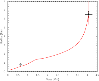
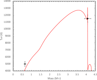
Figure 10: Locations of the components of PU Pup in the mass-radius diagram (top panel) and mass–$T_{\rm eff}$ (effective temperature) diagram (bottom panel). The Padova isochrone line of 170 My for Z = 0.014 (Bressan et al. 2012) is indicated by the red line. The filled and open circle symbols represent primary and secondary components, respectively. Vertical and horizontal lines show error bars of the measured quantities.

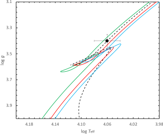
Figure 11: Location of the primary component of PU Pup in the $\log T_{\rm eff}-\log g$ diagram. The Padova evolutionary tracks (Bressan et al. 2012) for its mass are plotted for Z = 0.010 (green line), 0.014 (red line) and 0.017 (blue line). The best-fitting isochrone of 170 Myr for Z = 0.014 is also indicated by the black dotted line.

7 Concluding Remarks

PU Pup is an extraordinary close binary system. From historic data, including that from the HIPPARCOS satellite, the light curve, apparently of EB ($\beta$ Lyrae) kind, suggested either a close early-type pair with a strong third light contribution, or an ellipsoidal variable. A preliminary fitting to the HIPPARCOS data yielded a Main Sequence pair containing a massive star with a third light of almost $50\%$ in the system (thus resembling the system V454 Car). However, our spectral observations of PU Pup in 2008, 2014 and 2015 ruled out such a high level of third light. Neither the spectrum of such a source nor that of the secondary is visible.

Further analysis of the HIPPARCOS data, together with the RV information, presented the secondary as a late-type Main Sequence dwarf, consistent with a low mass ratio (for details, see Budding et al. 2019)). This model pointed to a low inclination, with the elliptical form of the primary component producing the dominant effect rather than eclipses. The light contribution of the secondary was estimated at less than a few percent of the total light.

The TESS satellite, launched in 2018, included 9 continuous cycles of PU Pup’s photometric light curve in its Sector 7 data. These very high accuracy observations reveal interesting small eclipse effects at the bottom of the light minima. The discovery of these small eclipses allows significant progress in uncovering the system’s parameters. The grazing eclipses constrain the system’s orbital inclination to be around 60 degrees. According to our revised model for the light and RV curves, PU Pup is approaching a semi-detached binary configuration, where it is the more massive primary that is close to filling its Roche limiting surface (cf. Kopal 1959, Chapter 7). This binary is thus moving towards the rarely seen ‘fast phase’ of interactive evolution.

Given the primary almost filling its lobe together and its over-sized secondary, PU Pup may be considered a near-Algol system. It could be considered similar to S Equulei (Plavec 1966, Qian & Zhu 2002), BH Virginis (Tian et al. 2008, Zeilik et al. 1990, Zhu et al. 2012), EG Cephei (Erdem et al. 2005, Zhu et al. 2009), and GQ Draconis (Atay et al. 2000, Qian et al. 2015). These systems have been reported to show signs of period variation. In some cases, these may be close to the end of a mass-transferring (RLOF) phase, and this might be the case for PU Pup. We are grateful to the unnamed referee for pointing out these comparable cases. This unusual system should therefore continue to be monitored closely for evidence of period variation or other indications of instability.

8 Acknowledgements

Generous allocations of time on the 1m McLennan Telescope and HERCULES spectrograph at the Mt John University Observatory in support of the Southern Binaries Programme have been made available through its TAC and supported by its Director, Dr. K. Pollard and previous Director, Prof. J. B. Hearnshaw. Useful help at the telescope were provided by the MJUO management (N. Frost and previously A. Gilmore & P. Kilmartin). Considerable assistance with the use and development of the hrsp software was given by its author Dr. J. Skuljan, and very helpful work with initial data reduction was carried out by R. J. Butland. We thank the anonymous referee for their guidance, which led to an improved paper.

General support for this programme has been shown by the the School of Chemical and Physical Sciences of the Victoria University of Wellington, as well as the Çanakkale Onsekiz Mart University, Turkey, notably Prof. O. Demircan. We thank the Royal Astronomical Society of New Zealand, particularly its Variable Stars South section (http://www.variablestarssouth.org), for support.

It is a pleasure to express our appreciation of the high-quality and ready availability, via the Mikulski Archive for Space Telescopes (MAST), of data collected by the TESS mission. Funding for the TESS mission is provided by the NASA Explorer Program. This research has made use of the SIMBAD data base, operated at CDS, Strasbourg, France, and of NASA’s Astrophysics Data System Bibliographic Services. We thank the University of Queensland for their assistance of collaboration tools.

9 Data availability

All data included in this article are available as listed in the paper or from the online supplementary material it cites.

Appendix A Table of Minima Times of PU Pup

Table A1: Times of Minima of PU Pup.

Time of Minimum	Uncertainty	Minimum	Reference	Remarks
(BJD)		Type
2448060.0709	0.0017	Min I	HIPPARCOS	(a)
2448061.3621	0.0020	Min II	HIPPARCOS	(a)
2448501.6288	0.0022	Min I	HIPPARCOS	(a)
2448502.9201	0.0020	Min II	HIPPARCOS	(a)
2457033.3148	0.0030	Min I	KWS I	(a)
2457034.6100	0.0020	Min II	KWS I	(a)
2457800.2415	0.0020	Min I	KWS V	(a)
2458134.6365	0.0025	Min II	KWS V	(a)
2458492.2724	0.0002	Min I	TESS	(b)
2458493.5724	0.0003	Min II	TESS	(b)
2458494.8609	0.0002	Min I	TESS	(b)
2458496.1505	0.0002	Min II	TESS	(b)
2458497.4410	0.0001	Min I	TESS	(b)
2458498.7320	0.0001	Min II	TESS	(b)
2458500.0263	0.0001	Min I	TESS	(b)
2458501.3156	0.0002	Min II	TESS	(b)
2458502.6036	0.0002	Min I	TESS	(b)
2458505.1885	0.0002	Min I	TESS	(b)
2458506.4824	0.0002	Min II	TESS	(b)
2458507.7658	0.0001	Min I	TESS	(b)
2458509.0614	0.0002	Min II	TESS	(b)
2458510.3554	0.0002	Min I	TESS	(b)
2458511.6458	0.0002	Min II	TESS	(b)
2458512.9341	0.0002	Min I	TESS	(b)
2458514.2267	0.0004	Min II	TESS	(b)
2458515.5190	0.0001	Min I	TESS	(b)

(a) These times of minima were derived using the theoretical LC templates.

(b) These times of minima were obtained from photometric observations directly.

Appendix B Example Spectrum of PU Pup

Figure B1: Example Plots of Spectral Orders chosen for line identifications of PU Pup. The échelle spectrum was taken on the night of December 03, 2015 and at orbital phase of 0.54. The lines used in RV measurements of PU Pup are indicated in each diagram. However, as indicated in Section 3.1 and Table 2, mostly strong lines of He I and Si II were used in the RV measurements.

References

- Atay et al. (2000) Atay, E., Alis, S., Keskin, M. M., Koksal, S., & Saygac, A. T., 2000, IBVS, 4988
- Bahcall (1980) Bahcall J. N., Soneira R. M., 1980, ApJS, 44, 73
- Bevington (1969) Bevington, P. R., 1969, Data Reduction and Analysis for the Physical Sciences, McGraw-Hill, New York
- Blackford et al. (2019) Blackford, M. G., Erdem, A., Sürgit, D., Özkardeş, B., Budding, E., Butland, R., & Demircan, O., 2019, MNRAS, 487, 161
- Bradstreet & Steelman (2002) Bradstreet, D. H., & Steelman, D. P., 2002, American Astronomical Society Meeting, 201, 7502
- Bressan et al. (2012) Bressan, A., Marigo, P., Girardi, L., Salasnich, B., Dal Cero, C., Rubele, S., & Nanni, A., MNRAS, 427, 127
- Budding & Zeilik (1995) Budding, E., & Zeilik, M., 1995, ApSS, 232, 355
- Budding & Demircan (2007) Budding, E., & Demircan, O., 2007, An Introduction to Astronomical Photometry, Cambridge Univ. Press
- Budding et al. (2009) Budding, E., Erdem, A., Innis, J. L., Olah, K., & Slee, O. B., 2009, AN, 330, 358
- Budding et al. (2019) Budding, E., Erdem, A., Sürgit, D., Özkardeş, B., Demircan, O., 2019, Journal of Occultation and Eclipse (JOE), 6, 40
- Chabrier et al. (2007) Chabrier, G., Gallardo, J., Baraffe I., 2007, A&A, 472, 17
- Claret (2017) Claret, A., 2017, A&A, 600, 30
- Erdem et al. (2005) Erdem, A., Budding, E., Demiran, O., Degirmenci, O.Ł., Gulmen, O. & Sezer, C., 2005, Astron. Nachr., 326, 332
- ESA (1997) ESA, 1997, The Hipparcos and Tycho Catalogues, ESA SP-1200
- Fabricius et al. (2002) Fabricius, C., Hog, E., Makarov, V. V., Mason, B. D., Wycoff, G. L., & Urban, S. E., 2002, A&A, 384, 180
- Flower (1996) Flower, P. J. 1996, ApJ, 469, 355
- Gaia Collaboration (2018) Gaia Collaboration, Brown, A. G. A., Vallenari, A., Prusti, T., et al., 2018, A&A, 616, 1
- Garrido et al. (2019) Garrido, H. E., Cruz, P., Diaz M. P., Aguliar, J. F., 2019, MNRAS, 482, 5379
- Garrison & Gray (1994) Garrison, R. F., & Gray, R. O., 1994, AJ, 104, 1556
- Ghedini (1982) Ghedini, S., 1982, Software for Photometric Astronomy, Willmann-Bell Publ. Corp, Richmond
- Hadrava (2004) Hadrava P., 2004, Publ. Astron. Inst. ASCR, 92, 15
- Hearnshaw et al. (2002) Hearnshaw J. B., Barnes S. I., Kershaw G. M., Frost N., Graham G., Ritchie R., Nankivell G. R., 2002, Exp. Astron., 13, 59
- Hosokawa (1958) Hosokawa, H., 1958, Sendai Astr. Raportoj., No 56, 226
- Jaschek et al. (1969) Jaschek, M., Jaschek, C., & Arnal, M., 1969, PASP, 81, 650
- Jenkins et al. (2016) Jenkins, J. M., Twicken, J. D., McCauliff, S., Campbell, J., Sanderfer, D., Lung, D., Mansouri-Samani, M., Girouard, F., Tenenbaum, P., Klaus, T., Smith, J. C., Caldwell, D. A., Chacon, A. D., Henze, C., Heiges, C., Latham, D. W., Morgan, E., Swade, D., Rinehart, S., & Vanderspek, R., 2016, SPIE 9913, 3, doi: 10.1117/12.2233418
- Kopal (1959) Kopal, Z., 1959, Close Binary Systems, Chapman & Hall, London
- Kraus et al. (2011) Kraus, A. L., Ireland, M. J., Martinache, F., & Hillenbrand, L.A., 2011, ApJ, 731, 8
- Kwee & van Woerden (1956) Kwee, K. K., & van Woerden, H., 1956, Bull. Astronomical Institutes of the Netherlands, Vol X11 (464), 327
- Lenz & Breger (2005) Lenz, P., & Breger, M. 2005, CoAst, 146, 53
- Maehara (2014) Maehara, H., 2014, Journal of Space Science Informatics Japan, 3, 119-127
- Marigo (2017) Marigo, P., Girardi L., Bressan A., Groenewegen M. A. T., Silva L., 2017, A&A, 482, 833
- Pecaut & Mamajek (2013) Pecaut, M.J., & Mamajek, E. E., 2013, ApJS, 208, 9
- Perryman et al. (1997) Perryman, M. A. C., Lindegren, L., Kovalevsky, J., Hog, E., Bastian, U., Bernacca, P. L., Creze, M., Donati, F., Grenon, M., Grewing, M., van Leeuwen, F., van der Marel, H., Mignard, F., Murray, C. A., Le Poole, R. S., Schrijver, H., Turon, C., Arenou, F., Froeschle, M., & Petersen, C. S., 1997, A&A, 500, 501
- Plavec (1966) Plavec, M., 1966, Bull. Astron. Inst. Czech., 17, 295
- Popper (1998) Popper, D. M., 1998, PASP, 110, 919
- Qian & Zhu (2002) Qian, -S. B., & Zhu, L. Y., 2002, ApJS, 142, 139
- Qian et al. (2015) Qian, S.-B, Zhou, X., Zhu, L. -Y., Zejda, M., Soonthornthum, E. -G., Zhao, E. -G., Zhang, J., Zhang, B., & Liao, W. -P., 2015, AJ, 150, 193
- Rhodes (2020) Rhodes, M. D., 2020, winfitter manual, https://michaelrhodesbyu.weebly.com/astronomy.html
- Ricker et al. (2014) Ricker, G. R., Winn, J. N., Vanderspek, R., Latham, D. W., Bakos, G. A., Bean, J. L., Berta-Thompson, Z. K., Brown, T. M., Buchhave, L., Butler, N. R., et al., 2014, Proc. SPIE Vol. 9143, doi: 10.1117/12.2063489
- Samus et al. (2017) Samus, N. N., Kazarovets, E. V., Durlevich, O. V., Kireeva, N. N., & Pastukhova, E. N., 2017 Astronomy Reports, 61, 80
- Schlafly & Finkbeiner (2011) Schlafly, E. F., & Finkbeiner, D. P., 2011, ApJ, 737, 103
- Skuljan (2014) Skuljan J., 2014, HERCULES Reduction Software Package (HRSP Version 5), private communication
- Skuljan (2020) Skuljan, J., 2020, HERCULES Reduction Software Package (HRSP Version 7), private communication
- Stift (1979) Stift, M. J., 1979, IBVS, 1540
- Stock et al. (2002) Stock, M. K., Stock, J., Garcia, J., & Sanchez, N., 2002, Rev. Mex. Astron. Astrofis, 38, 127
- Svechnikov & Kuznetsova (1990) Svechnikov, M. A., & Kuznetsova, Eh. F. 1990, Catalogue of approximate photometric and absolute elements of eclipsing variable stars, Vols. 1-2, Sverdlovsk, Ural University
- Tian et al. (2008) Tian, Y.-P., Xiang, F.-Y., & Tao, X., 2008, Publ. Astron. Soc. Jap., 60
- Torres et al. (2010) Torres, G., Andersen, J., Giménez, A., 2010, A&ARv, 18, 67
- Tunçel Güçtekin et al. (2016) Tunçel Güçtekin, S., Bilir, S., Karaali, S., Ak, S., Ak, T., Bostancı, Z. F., 2016, Ap&SS, 361, 186
- van den Bos (1927) van den Bos, W. H., 1927, BAN, 4, 45
- van Leeuwen (2007) van Leeuwen, F., 2007, A&A, 474, 653
- Wilson & Devinney (1971) Wilson, R. E., & Devinney, E. J., 1971, ApJ, 166, 605
- Worley & Douglas (1997) Worley, C. E., & Douglas, G. G., 1997, The Washington Visual Double Star Catalog, Publ. US Naval Observatory, Washington.
- Zasche et al. (2014) Zasche, P., Wolf, M., Vrastil, J., Liska, J., Skarka, M., & Zejda, M., 2014, A&A, 572, A71
- Zeilik et al. (1990) Zeilik, M., Ledlow, M., Rhodes, M. D., Arevalo, M. J., & Budding, E., 1990 Astrophys. J., 354, 352-358
- Zhu et al. (2009) Zhu, L.- Y., Qian, S. -B., Liao, W. P., Miloslav, Z., & Zdenek, M., 2009, PASJ, 61, 529
- Zhu et al. (2012) Zhu, L., Qian, S. -B., & Li, L., 2012, PASJ, 64, 94
- Zola et al. (2004) Zola, S., Rucinski, S.M., Baran, A., et al., 2004, Acta Astron. 54, 299