Accuracy on the Line: On the Strong Correlation
Between Out-of-Distribution and In-Distribution Generalization

Abstract

For machine learning systems to be reliable, we must understand their performance in unseen, out-of-distribution environments. In this paper, we empirically show that out-of-distribution performance is strongly correlated with in-distribution performance for a wide range of models and distribution shifts. Specifically, we demonstrate strong correlations between in-distribution and out-of-distribution performance on variants of CIFAR-10 & ImageNet, a synthetic pose estimation task derived from YCB objects, satellite imagery classification in FMoW-WILDS, and wildlife classification in iWildCam-WILDS. The strong correlations hold across model architectures, hyperparameters, training set size, and training duration, and are more precise than what is expected from existing domain adaptation theory. To complete the picture, we also investigate cases where the correlation is weaker, for instance some synthetic distribution shifts from CIFAR-10-C and the tissue classification dataset Camelyon17-WILDS. Finally, we provide a candidate theory based on a Gaussian data model that shows how changes in the data covariance arising from distribution shift can affect the observed correlations.

.tocmtsection

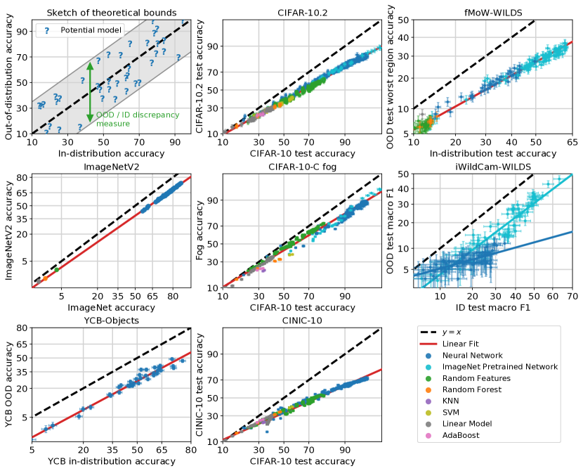
Figure 1: Out-of-distribution accuracies vs. in-distribution accuracies for a wide range of models, datasets, and distribution shifts. Top left: A sketch of the current bounds from domain adaptation theory. These bounds depend on distributional distances between in-distribution and out-of-distribution data, and they are loose in that they limit the deviation away from the y = x diagonal but do not prescribe a specific trend within these wide bounds (see Section 8). Remaining panels: In contrast, we show that for a wide range of models and datasets, there is a precise linear trend between out-of-distribution accuracy and in-distribution accuracy. Unlike what we might expect from theory, the linear trend does not follow the $y=x$ diagonal. The different panels represent different pairs of in-distribution and out-of-distribution datasets. Within each panel, we plot the performances of many different models, with different model architectures and hyperparameters. These datasets capture a variety of distribution shifts from dataset reproduction (CIFAR-10.2, ImageNet-V2); a real-world spatiotemporal distribution shift on satellite imagery (FMoW-WILDS); using a different benchmark test dataset (CINIC-10); synthetic perturbations (CIFAR-10-C and YCB-Objects); and a real-world geographic shift in wildlife monitoring (iWildCam-WILDS). Interestingly, for iWildCam-WILDS, models pretrained on ImageNet follow a different linear trend than models trained from scratch in-distribution, and we plot a separate trend line for ImageNet pretrained models in the iWildCam-WILDS panel. We explore this phenomenon more in Section 5.

1 Introduction

Machine learning models often need to generalize from training data to new environments. A kitchen robot should work reliably in different homes, autonomous vehicles should drive reliably in different cities, and analysis software for satellite imagery should still perform well next year. The standard paradigm to measure generalization is to evaluate a model on a single test set drawn from the same distribution as the training set. But this paradigm provides only a narrow in-distribution performance guarantee: a small test error certifies future performance on new samples from exactly the same distribution as the training set. In many scenarios, it is hard or impossible to train a model on precisely the distribution it will be applied to. Hence a model will inevitably encounter out-of-distribution data on which its performance could vary widely compared to in-distribution performance. Understanding the performance of models beyond the training distribution therefore raises the following fundamental question: how does out-of-distribution performance relate to in-distribution performance?

Classical theory for generalization across different distributions provides a partial answer [71, 8]. For a model $f$ trained on a distribution $D$, known guarantees typically relate the in-distribution test accuracy on $D$ to the out-of-distribution test accuracy on a new distribution $D^{\prime}$ via inequalities of the form

$$|\text{acc}_{D}(f)-\text{acc}_{D^{\prime}}(f)|\;\leq\;d(D,D^{\prime})$$

where $d$ is a distance between the distributions $D$ and $D^{\prime}$ such as the total variation distance. Qualitatively, these bounds suggest that out-of-distribution accuracy may vary widely as a function of in-distribution accuracy unless the distribution distance $d$ is small and the accuracies are therefore close (see Figure 1 (top-left) for an illustration). More recently, empirical studies have shown that in some settings, models with similar in-distribution performance can indeed have different out-of-distribution performance [72, 119, 30].

In contrast to the aforementioned results, recent dataset reconstructions of the popular CIFAR-10, ImageNet, MNIST, and SQuAD benchmarks showed a much more regular pattern [86, 73, 114, 66]. The reconstructions closely followed the original dataset creation processes to assemble new test sets, but small differences were still enough to cause substantial changes in the resulting model accuracies. Nevertheless, the new out-of-distribution accuracies are almost perfectly linearly correlated with the original in-distribution accuracies for a range of deep neural networks. Importantly, this correlation holds despite the substantial gap between in-distribution and out-of-distribution accuracies (see Figure 1 (top-middle) for an example). However, it is currently unclear how widely these linear trends apply since they have been mainly observed for dataset reproductions and common variations of convolutional neural networks.

In this paper, we conduct a broad empirical investigation to characterize when precise linear trends such as in Figure 1 (top-middle) may be expected, and when out-of-distribution performance is less predictable as in Figure 1 (top-left). Concretely, we make the following contributions:

• We show that precise linear trends occur on several datasets and associated distribution shifts (see Figure 1). Going beyond the dataset reproductions in earlier work, we find linear trends on

  • popular image classification benchmarks (CIFAR-10 [57], CIFAR-10.1 [86], CIFAR-10.2 [66], CIFAR-10-C [46], CINIC-10 [32], STL-10 [27], ImageNet [33], ImageNet-V2 [86]),

  • a pose estimation testbed based on YCB-Objects [17],

  • and two distribution shifts derived from concrete applications of image classification: satellite imagery and wildlife photos via the FMoW-WILDS and iWildCam-WILDS variants from WILDS [25, 6, 55].

• We show that the linear trends hold for many models ranging from state-of-the-art methods such as convolutional neural networks, visual transformers, and self-supervised models, to classical methods like logistic regression, nearest neighbors, and kernel machines. Importantly, we find that classical methods follow the same linear trend as more recent deep learning architectures. Moreover, we demonstrate that varying model or training hyperparameters, training set size, and training duration all result in models that follow the same linear trend.

• We also identify three settings in which the linear trends do not occur or are less regular: some of the synthetic distribution shifts in CIFAR-10-C (e.g., Gaussian noise), the Camelyon17-WILDS shift of tissue slides from different hospitals, and a version of the aforementioned iWildCam-WILDS wildlife classification problem with a different in-distribution train-test split [6]. We analyze these cases in detail via additional experiments to pinpoint possible causes of the linear trends.

• Pre-training a model on a larger and more diverse dataset offers a possibility to increase robustness. Hence we evaluate a range of models pre-trained on other datasets to study the impact of pre-training on the linear trends. Interestingly, even pre-trained models sometimes follow the same linear trends as models trained only on the in-distribution training set. Two examples are ImageNet pre-trained models evaluated on CIFAR-10 and FMoW-WILDS. In other cases (e.g., iWildCam-WILDS), pre-training yields clearly different relationships between in-distribution and out-of-distribution accuracies.

• As a starting point for theory development, we provide a candidate theory based on a simple Gaussian data model. Despite its simplicity, this data model correctly identifies the covariance structure of the distribution shift as one property affecting the performance correlation on the Gaussian noise corruption from CIFAR-10-C.

Overall, our results show a striking linear correlation between the in-distribution and out-of-distribution performance of many models on multiple distribution shifts. This raises the intriguing possibility that, despite their different creation mechanisms, a diverse range of distribution shifts may share common phenomena. In particular, improving in-distribution performance reliably improves out-of-distribution performance as well. However, it is currently unclear whether improving in-distribution performance is the only way, or even the best way, to improve out-of-distribution performance. More research is needed to understand the extent of the linear trends observed in this work and whether robustness interventions can improve over the baseline given by empirical risk minimization. We hope that our work serves as a step towards a better understanding of distribution shift and how we can train models that perform robustly out-of-distribution.

Paper outline.

Next, we introduce our main experimental framework that forms the backbone of our investigation. The following sections instantiate this framework for multiple distribution shifts.

Section 3 shows results on a wide range of distribution shifts where precise linear trends do occur. Section 4 then turns to distribution shifts where the linear trends are less regular or do not exist. Section 5 investigates the role of pretraining in more detail since models pre-trained on a different dataset sometimes – but not always – deviate from the linear trends.

After our experiments, we briefly summarize the empirical phenomena in Section 6 and then present our theoretical model in Section 7. Section 8 describes related work and Section 9 concludes with a discussion of our results, possible implications for research on reliable machine learning, and directions for future work.

2 Experimental setup

In each of our main experiments, we compare performance on two data distributions. The first is the training distribution $D$, which we refer to as “in-distribution” (ID). Unless noted otherwise, all models are trained only on samples from $D$ (the main exception is pre-training on a different distribution). We compute ID performance via a held-out test set sampled from $D$. The second distribution is the “out-of-distribution” (OOD) distribution $D^{\prime}$ that we also evaluate the models on. For a loss function $\ell$ (e.g., error or accuracy), we denote the loss of model $f$ on distribution $D$ with $\ell_{D}(f)=\mathbb{E}_{x,y\sim D}\left[\ell(f(x),y)\right]$.

Experimental procedure.

The goal of our paper is to understand the relationship between $\ell_{D}(f)$ and $\ell_{D^{\prime}}(f)$ for a wide range of models $f$ (convolutional neural networks, kernel machines, etc.) and pairs of distributions $D,D^{\prime}$ (e.g., CIFAR-10 and the CIFAR-10.2 reproduction). Hence for each pair $D,D^{\prime}$, our core experiment follows three steps:

1. Train a set of models $\{f_{1},f_{2},\ldots\}$ on samples drawn from $D$. Apart from the shared training distribution, the models are trained independently with different training set sizes, model architectures, random seeds, optimization algorithms, etc.

2. Evaluate the trained models $f_{i}$ on two test sets drawn from $D$ and $D^{\prime}$, respectively.

3. Display the models $f_{i}$ in a scatter plot with each model’s two test accuracies on the two axes to inspect the resulting correlation.

An important aspect of our scatter plots is that we apply a non-linear transformation to each axis. Since we work with loss functions bounded in $[0,1]$, we apply an axis scaling that maps $[0,1]$ to $[-\infty,+\infty]$ via the probit transform. The probit transform is the inverse of the cumulative density function (CDF) of the standard Gaussian distribution, i.e., $l_{\text{transformed}}=\Phi^{-1}(l)$. Transformations like the probit or closely related logit transform are often used in statistics since a quantity bounded in $[0,1]$ can only show linear trends for a bounded range. The linear trends we observe in our correlation plots are substantially more precise with the probit (or logit) axis scaling. Unless noted otherwise, each point in a scatter plot is a single model (not averaged over random seeds) and we show each point with 95% Clopper-Pearson confidence intervals for the accuracies.

We assembled a unified testbed that is shared across experiments and includes a multitude of models ranging from classical methods like nearest neighbors, kernel machines, and random forests to a variety of high-performance convolutional neural networks. Our experiments involved more than 3,000 trained models and 100,000 test set evaluations of these models and their training checkpoints. Due to the size of these experiments, we defer a detailed description of the testbed used to Appendix A.

3 The linear trend phenomenon

In this section, we show precise linear trends between in-distribution and out-of-distribution performance occur across a diverse set of models, data domains, and distribution shifts. Moreover, the linear trends holds not just across variations in models and model architectures, but also across variation in model or training hyperparameters, training dataset size, and training duration.

ID Dataset	OOD Dataset	$R^{2}$ of linear fit (probit domain)	Number of models evaluated
CIFAR-10	CIFAR-10.1	0.995	1,060
	CIFAR-10.2	0.997	1,060
	CINIC-10	0.991	949
	STL-10	0.995	456
	CIFAR-10-C Fog	0.990	790
	CIFAR-10-C Brightness	0.940	519
ImageNet	ImageNet-V2	0.996	219
YCB-Objects	YCB-Objects OOD	0.975	39
iWildCam-WILDS ID	iWildCam-WILDS OOD	0.881 (0.536)	66 (63)
FMoW-WILDS ID	FMoW-WILDS OOD	0.984	162

Table 1: Summary of ID and OOD pairs where we observe precise linear trends in our experiments. Number of models evaluated is the number of models trained on the ID training set, evaluated on the ID and OOD test sets, and used to compute the linear fits. For brevity, we list only two CIFAR-10-C shifts; see Appendix C.2 for a complete list. As discussed in Section 5, on iWildCam-WILDS, ImageNet pretrained models exhibit a different linear trend than models trained from scratch. Therefore, for iWildCam-WILDS, we report the number of models and $R^{2}$ for pretrained models and models trained from scratch (given in parentheses) separately.

3.1 Distribution shifts with linear trends

We find linear trends for models in our testbed trained on five different datasets—CIFAR-10, ImageNet, FMoW-WILDS, iWildCam-WILDS, and YCB-Objects—and evaluated on distribution shifts that fall into four broad categories. These trends are summarized in Table 1.

Dataset reproduction shifts. Dataset reproductions involve collecting a new test set by closely matching the creation process of the original. Distribution shift arises as a result of subtle differences in the dataset construction pipelines. Recent examples of dataset reproductions are the CIFAR-10.1 and ImageNet-V2 test sets from Recht et al. [86], who observed linear trends for deep models on these shifts. In Figure 1, we extend this result and show both deep and classical models trained on CIFAR-10 and evaluated on CIFAR-10.2 [66] follow a linear trend. In Appendix B, we further show linear trends occur for deep and classical CIFAR-10 models evaluated on CIFAR-10.1 and for ImageNet models evaluated on ImageNet-V2.

Distribution shifts between machine learning benchmarks. We also consider distribution shifts between distinct benchmarks which are drawn from different data sources, but which use a compatible set of labels. For instance, both CIFAR-10 and CINIC-10 [32] use the same set of labels, but CIFAR-10 is drawn from TinyImages [108] and CINIC-10 is drawn from ImageNet [33] images. We show CIFAR-10 models exhibit linear trends when evaluated on CINIC-10 (Figure 1) or on STL-10 [27] (Appendix B).

Synthetic perturbations. Synthetic distribution shifts arise from applying a perturbation, such as adding Gaussian noise, to existing test examples. CIFAR-10-C [46] applies 19 different synthetic perturbations to the CIFAR-10 test set. For many of these perturbations, we observe linear trends for CIFAR-10 trained models, e.g. the Fog shift in Figure 1. However, there are several exceptions, most notably adding isotropic Gaussian noise. We give further examples of linear trends on synthetic CIFAR-10-C shifts in Appendix B, and we more thoroughly discuss non-examples of linear trends in Section 4. In Figure 1, we also show that pose-estimation models trained on rendered images of YCB-Objects [17] follow a linear trend when evaluated on a images rendered with perturbed lighting and texture conditions.

Distribution shifts in the wild. We also find linear trends on two of the real-world distribution shifts from the WILDS benchmark [55]: FMoW-WILDS and iWildCam-WILDS. FMoW-WILDS is a satellite image classification task derived from Christie et al. [25] where in-distribution data is taken from regions (e.g., the Americas, Africa, Europe) across the Earth between 2002 and 2013, the out-of-distribution test-set is sampled from each region during 2016 to 2018, and models are evaluated by their accuracy on the worst-performing region. In Figure 1, we show models trained on FMoW-WILDS exhibit linear trends when evaluated out-of-distribution under both of these temporal and subpopulation distribution shifts.

iWildCam-WILDS is an image dataset of animal photos taken by camera traps deployed in multiple locations around the world [55, 6]. It is a multi-class classification task, where the goal is to identify the animal species (if any) within each photo. The held-out test set comprises photos taken by camera traps that are not seen in the training set, and the distribution shift arises because different camera traps vary markedly in terms of angle, lighting, and background. In Figure 1, we show models trained on iWildCam-WILDS also exhibit linear trends when evaluated OOD across different camera traps.

3.2 Variations in model hyperparameters, training duration, and training set size

Figure 2: The linear trend between ID and OOD accuracy is invariant to changes in model hyperparameters, the number of training steps, and training set size. In each panel, we compare models with the linear fit from Figure 1. Left: For each model family, we vary model-size, regularization, and optimization hyperparameters. Middle: We evaluate each network after every epoch of training. Right: We train models on randomly sampled subsets of the training data, ranging from 1% to 80% of the CIFAR-10 training set size. In each setting, variation in hyperparameters, training duration, or training set size moves models along the trend line, but does not affect the linear fit.

The linear trends we observe hold not just across different models, but also across variation in model and optimization hyperparameters, training dataset size, and training duration.

In Figure 2, we train and evaluate both classical and neural models on CIFAR-10 and CIFAR-10.2 while systematically varying (1) model hyperparameters, (2) training duration, and (3) training dataset size. When varying hyperparameters controlling the model size, regularization, and the optimization algorithm, the model families continue to follow the same trend line ($R^{2}=0.99$). We also find models lie on the same linear trend line throughout training ($R^{2}=0.99$). Finally, we observe models on trained on random subsets of CIFAR-10 lie on the same linear trend line as models trained on the full CIFAR-10 training set, despite their corresponding drop in in-distribution accuracy ($R^{2}=0.99$). In each case, hyperparameter tuning, early stopping, or changing the amount of i.i.d. training data moves models along the trend line, but does not alter the linear fit.

While we focus here on CIFAR-10 models evaluated on CIFAR-10.2, in Appendix B, we conduct an identical set of experiments for CINIC-10, CIFAR-10-C Fog, YCB-Objects, and FMoW-WILDS. We find the same invariance to hyperparameter, dataset size, and training duration shown in Figure 2 also holds for these diverse collection of datasets.

4 Distribution shifts with weaker correlations

We now investigate distribution shifts with a weaker correlation between ID and OOD performance than the examples presented in the previous section. We will discuss the Camelyon17-WILDS tissue classification dataset and specific image corruptions from CIFAR-10-C. Further discussion of a version of the iWildCam-WILDS wildlife classification dataset with a different in-distribution train-test split can be found in Appendix C.3.

4.1 Camelyon17-WILDS

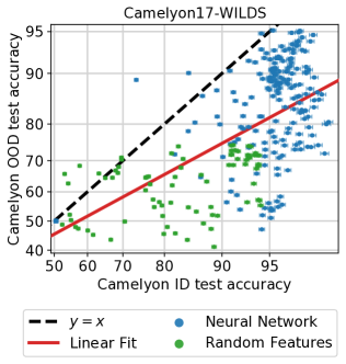
Figure 3: A range of neural network and random feature models trained on Camelyon17-WILDS and evaluated on the ID and OOD test sets. OOD accuracy is highly variable across the spectrum of ID accuracies, and there is no precise linear trend.

Camelyon17-WILDS [4, 55] is an image dataset of metastasized breast cancer tissue samples collected from different hospitals. It is a binary image classification task where each example is a tissue patch. The corresponding label is whether the patch contains any tumor tissue. The held-out OOD test set contains tissue samples from a hospital not seen in the training set. The distribution shift largely arises from differences in staining and imaging protocols across hospitals.

In Figure 3, we plot the results of training different ImageNet models and random features models from scratch across a variety of random seeds. There is significant variation in OOD performance. For example, the models with 95% ID accuracy have OOD accuracies that range from about 50% (random chance) to 95%. This high degree of variability holds even after averaging each model over ten independent training runs (see Appendix C.1).

Appendix C.1 also contains additional analyses exploring the potential sources of OOD performance variation, including ImageNet pretraining, data augmentation, and similarity between test examples. Specifically, we observe that ImageNet pretraining does not increase the ID-OOD correlation, while strong data augmentation significantly reduces, but does not eliminate, the OOD variation. Another potential reason for the variation is the similarity between images from the same slide / hospital, as similar examples have been shown to result in analogous phenomena in natural language processing [119]. We explore this hypothesis in a synthetic CIFAR-10 setting, where we simulate increasing the similarity between examples by taking a small seed set of examples and then using data augmentations to create multiple similar versions. We find that in this CIFAR-10 setting, shrinking the effective test set size in this way increases OOD variation to a substantially greater extent than shrinking the effective training set size.

4.2 CIFAR-10-Corrupted

CIFAR-10-C [46] corrupts the CIFAR-10 test set with various image perturbations. The choice of corruption can have a significant impact on the correlation between ID and OOD accuracy. Appendix C.2 provides plots and $R^{2}$ values for each corruption. We already showed an example of one of the more precise fits, fog corruption, in Figure 1 (bottom middle). Interestingly, the mathematically easy to describe corruption with Gaussian noise is one of the corruptions with worst ID-OOD correlation (see Figure 4 left).

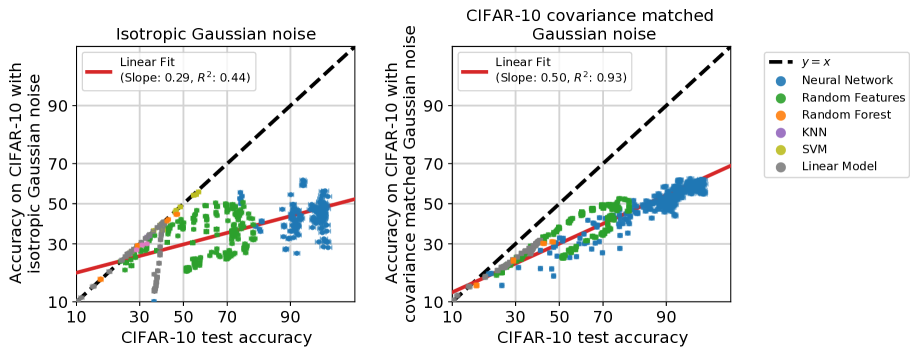
Figure 4: When the out-of-distribution data covariance matches the in-distribution data covariance, the linear fit is significantly better. Left: A collection of models trained on CIFAR-10 and evaluated in-distribution on CIFAR-10 and out-of-distribution on CIFAR-10 images corrupted with isotropic Gaussian noise. Right: The same collection of models evaluated out-of-distribution on CIFAR-10 images corrupted with Gaussian noise with the same covariance as CIFAR-10.

We also investigate how the relationship between the ID and OOD data covariances impacts the linear trend. The theoretical model discussed in Section 7 predicts linear fits occur if the data covariances between ID and OOD are the same up to a constant scaling factor. Thus, in Figure 4, we compare adding isotropic Gaussian noise to the CIFAR-10 test set versus adding Gaussian noise with the same covariance as data examples from CIFAR-10. We find that when the OOD covariance matches the ID covariance the linear fit is substantially better ($R^{2}=0.93$ vs. $R^{2}=0.44$). This finding is consistent with the theoretical model we propose and discuss in Section 7.

In Appendix C.2, we also compare CIFAR-10-C to ImageNet-C and notice that each corruption displays a more linear trend on ImageNet-C compared to CIFAR-10-C. Investigating this discrepancy further is an interesting direction for future work.

5 The effect of pretrained models

In this section, we expand our scope to methods that leverage models pretrained on a third auxiliary distribution different from the ones we refer to in-distribution (ID) and out-of-distribution (OOD). Fine-tuning pretrained models on the task-specific (ID) training set is a central technique in modern machine learning [36, 84, 56, 77, 34], and zero-shot prediction (using the pretrained model directly without any task-specific training) is showing increasing promise as well [15, 80]. Therefore, it is important to understand how the use of pretrained models affects the robustness of models to OOD data, and whether fine-tuning and zero-shot inference differ in that respect.

The dependence of the pretrained model on auxiliary data makes the ID/OOD distinction more subtle. Previously, “ID” simply referred to the distribution of the training set, while OOD referred to an alternative distribution not seen in training. In this section, the training set includes the auxiliary data as well, but we still refer to the task-specific training set distributions as ID. This means, for example, that when fine-tuning an ImageNet model on the CIFAR-10 training set, we still refer to accuracy on the CIFAR-10 test set as ID accuracy. In other words, the “ID” distributions we refer to in this section are precisely the “ID” distributions of the previous sections (displayed on the $x$-axes in our scatter plots), but the presence of auxiliary training data alters the meaning of the term.

With the effect of auxiliary data on the meaning of “ID” in mind, it is reasonable to expect that ID/OOD linear trends observed when training purely on ID data will change or break down when pretrained models are used. In this section we test this hypothesis empirically and reveal a more nuanced reality: the task and the use of the pretrained model matter, and sometimes models pre-trained on seemingly broader distributions still follow the same linear trend as the models trained purely on in-distribution data. We first present our findings for fine-tuning pretrained ImageNet models and subsequently discuss results for zero-shot prediction. See Appendix D for more experimental details.

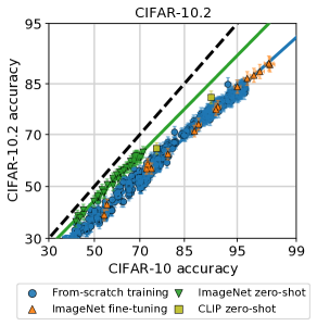
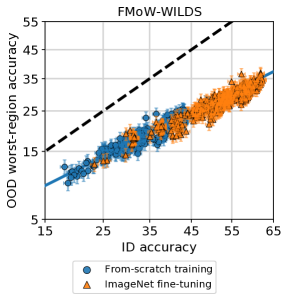
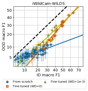
Figure 5: The effect of pre-training with additional data on CIFAR-10.2 (left), FMoW-WILDS (middle), and iWildCam-WILDS (right). On CIFAR-10.2 and FMoW-WILDS, fine-tuning pretrained models moves the models along the predicted ID-OOD line. However, on CIFAR-10.2, zero-shot prediction using pretrained models deviates from this line. On iWildCam-WILDS, fine-tuning pretrained models changes the ID-OOD relationship observed for models trained from scratch. Moreover, the weight decay hyperparameter affects the ID-OOD relationship in fine-tuned models.

Fine-tuning pretrained models on ID data.

Figure 5 plots OOD performance vs. ID performance for models trained from-scratch (purely on ID data) and fine-tuned models whose initialization was pretrained on ImageNet. Across the board, pretrained models attain better performance on both the ID and OOD test sets. However, fine-tuning affects ID-OOD correlations differently across tasks. In particular, for CIFAR-10 reproductions and for FMoW-WILDS, fine-tuning produces results that lie on the same ID-OOD trend as purely ID-trained models (Figure 5 left and center). On the other hand, a similar fine-tuning procedure yields models with a different ID-OOD relationship on iWildCam-WILDS than models trained from scratch on this dataset. Moreover, the weight decay used for fine-tuning seems to also affect the linear trend (Figure 5 right).

One conjecture is that the qualitatively different behavior of fine-tuning on iWildCam-WILDS is related to the fact that ImageNet is a more diverse dataset that may encode robustness-inducing invariances that are not represented in the iWildCam-WILDS ID training set. For instance, both ImageNet and iWildCam-WILDS contain high-resolution images of natural scenes, but the camera perspectives in iWildCam-WILDS may be more limited compared to ImageNet. Hence ImageNet classifiers may be more invariant to viewpoint, which may aid generalization to previously unseen camera viewpoints in the OOD test set of iWildCam-WILDS. On the other hand, the satellite images in FMoW-WILDS are all taken from an overhead viewpoint, so learning invariance to camera viewpoints from ImageNet might not be as beneficial. Investigating this and related conjectures (e.g., invariances such as lighting, object pose, and background) is an interesting direction for future work.

Zero-shot prediction on pretrained models.

A common explanation for OOD performance drop is that training on the ID training set biases the model toward patterns that are more predictive on the ID test set than on its OOD counterpart. With that explanation in mind, the fact that fine-tuned models maintain the same ID/OOD linear trend as from-scratch models is surprising: once could reasonably expect that an initialization determined independently of either ID or OOD data would produce models that are less biased toward the former. Indeed, in the extreme scenario that no fine-tuning takes place, the model should have no bias toward either distribution, and we therefore expect to see a different ID/OOD trend.

The CIFAR-10 allows us directly test this expectation directly by performing zero-shot inference on models pretrained on ImageNet: since the CIFAR-10 classes form a subset of the ImageNet classes, we simply feed (resized) CIFAR-10 images to these models, and limit the prediction to the relevant class subset. The resulting classifiers have no preference for either the ID or OOD test set because they depend on neither distribution. We plot the zero-shot prediction results in Figure 5 (left) and observe that, as expected, they deviate from the basic linear trend. Moreover, they form a different linear trend closer—but not identical—to $x=y$. The fact that the zero-shot linear trend is closer to $x=y$ supports the hypothesis that the performance drop partially stems from bias in ID training. However, the fact that this trend is still below $x=y$ suggests that the drop is also partially due to CIFAR-10 reproductions being harder than CIFAR-10 for current methods (interestingly, humans show similar performance on both test sets [86, 73, 95]). These finding agree with prior work [66].

As another test of zero-shot inference, we apply two publically-available CLIP models on CIFAR-10 by creating last-layer weights out of natural language descriptions of the classes [80]. As Figure 5 (left) shows, these models are slightly above the basic ID/OOD linear trend, but below the trend of zero-shot inference with ImageNet models.

Additional experiments.

In Appendix D we describe additional experiments with pretrained models. To explore a middle ground between zero-shot prediction and full-model fine-tuning, we consider a linear probe on CLIP for both CIFAR-10 and FMoW-WILDS. For CIFAR-10, we also consider models trained on a task-relevant subset of ImageNet classes [32] and models trained in a semi-supervised fashion using unlabeled data from 80 Million Tiny Images [108, 18, 2]. Generally, we find that, compared to zero-shot prediction, these techniques deviate less from the basic linear trend. We also report results on additional OOD settings, namely CIFAR-10.1 and different region subsets for FMoW-WILDS, and reach similar conclusions.

6 Summary of empirical phenomena

The previous sections have presented a variety of empirical phenomena concerning the relationship between in-distribution and out-of-distribution performance. To summarize these phenomena, we now briefly highlight the key observations. These observations will also guide the development of our theoretical model of distribution shift in the next section.

The key observations are:

1. The linear trend between in-distribution and out-of-distribution performance applies to a wide range of model families and holds under variation in architecture, hyperparameters, and training duration (Section 3).

2. The linear trends are more precise after applying a probit or logit scaling on both axes of the scatter plotes.

3. Changing the amount of in-distribution training data does not affet the linear trend (Section 3.2). On the other hand, pre-training on a different data distribution can – but does not always – yield a different trend (Section 5).

4. Some distribution shifts show precise linear trends while others do so only for subsets of models or not at all (Section 4).

7 Theoretical models for linear fits

In this section we propose and analyze a simple theoretical model that distills several of the empirical phenomena from the previous sections. Our goal here is not to obtain a general model that encompasses complicated real distributions such as the images in CIFAR-10. Instead, our focus is on finding a simple model that is still rich enough to exhibit some of the same phenomena as real data distributions.

7.1 A simple Gaussian distribution shift setting

We consider a simple binary classification problem where the label $y$ is distributed uniformly on $\{-1,1\}$ both in the original distribution $D$ and shifted distribution $D^{\prime}$. Conditional on $y$, we consider $D$ such that $\boldsymbol{x}\in\mathbb{R}^{d}$ is an isotropic Gaussian, i.e.,

$$\boldsymbol{x}\,|\,y\;\sim\;\mathcal{N}(\boldsymbol{\mu}\cdot y;\,\sigma^{2}I_{d\times d}),$$

for mean vector $\boldsymbol{\mu}\in\mathbb{R}^{d}$ and variance $\sigma^{2}>0$.

We model the distribution shift as a change in $\sigma$ and $\boldsymbol{\mu}$. Specifically, we assume that the shifted distribution $D^{\prime}$ corresponds to shifted parameters

$$\boldsymbol{\mu}^{\prime}=\alpha\cdot\boldsymbol{\mu}+\beta\cdot\boldsymbol{\Delta}~{}~{}\quad\mbox{and}\quad~{}~{}\sigma^{\prime}=\gamma\cdot\sigma$$ (1)

where $\alpha,\beta,\gamma>0$ are fixed scalars and $\boldsymbol{\Delta}$ is uniformly distributed on the sphere in $\mathbb{R}^{d}$. Note that in our setting $D^{\prime}$ is a random object determined by the draw of $\boldsymbol{\Delta}$.

Within the setup describe above, we focus on linear classifiers of the form $\boldsymbol{x}\mapsto\operatorname{\mathrm{sign}}(\boldsymbol{\theta}^{\top}\boldsymbol{x})$. The following theorem states that, as long as $\boldsymbol{\theta}$ depends only on the training data and is thereby independent of the random shift direction $\boldsymbol{\Delta}$, the probit-transformed accuracies on $D$ and $D^{\prime}$ have a near-linear relationship with slope $\alpha/\gamma$. (Recall that the probit transfrom is the inverse of the standard Normal cdf $\Phi(x)=\int_{-\infty}^{x}\frac{1}{\sqrt{2\pi}}e^{-t^{2}/2}\mathrm{d}t$). The deviation from linearity is of order $d^{-1/2}$ and vanishes in high dimension.

Theorem 1.

In the setting described above where $\boldsymbol{\Delta}$ is independent of $\boldsymbol{\theta}$, let $\delta\in(0,1)$. With probability at least $1-\delta$, we have

$$\left\lvert\Phi^{-1}\left(\mathrm{acc}_{D^{\prime}}(\boldsymbol{\theta})\right)-\frac{\alpha}{\gamma}\,\Phi^{-1}\left(\mathrm{acc}_{D}(\boldsymbol{\theta})\right)\right\rvert\;\leq\;\frac{\beta}{\gamma\sigma}\sqrt{\frac{2\log\nicefrac{{2}}{{\delta}}}{d}}\;.$$

The theorem is a direct consequence of the concentration of measure; see proof in Appendix E.1.

We illustrate Theorem 1 by simulating its setup and training different linear classifiers by varying the loss function and regularization. Figure 6 shows good agreement between the performance of linear classifiers and the theoretically-predicted linear trend. Furthermore, conventional nonlinear classifiers (nearest neighbors and random forests) also satisfy the same linear relationship, which does not directly follow from our theory. Nevertheless, if the decision boundary of the nonlinear becomes nearly linear in our setting a similar theoretical analysis might be applicable. Our simple Gaussian setup thus illustrates how linear trends can arise across a wide range of models.

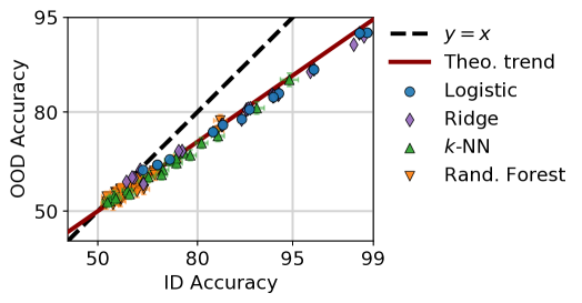
Figure 6: Illustration of the theoretical distribution shift model in Section 7.1 with $d=10^{5}$, $\alpha=0.7$, $\beta=0.5$ and $\gamma=1$ (see Appendix E.3 for details). The accuracies for linear models (logistic and ridge regression) agree with the prediction of Theorem 1. Moreover, nonlinear models (nearest neighbors and random features) exhibit the same probit trend we prove for linear classifiers.

7.2 Modeling departures from the linear trend

In the previous section, we identified a simple Gaussian setting that showed linear fits across a large range of models. Now we discuss small changes to the setting that break linear trends and draw parallels to the empirical observations on complex datasets presented in this paper. In Appendix E.2, we discuss each of these modifications in further detail.

Adversarial distribution shifts. Previously, the direction $\boldsymbol{\Delta}$ which determines the distribution shift as defined above in eq. (1), was chosen independent of the tested models $\boldsymbol{\theta}_{1},\ldots,\boldsymbol{\theta}_{k}$. However, when $\boldsymbol{\Delta}$ is instead chosen by an adversary with knowledge of the tested models, the ID-OOD relationship can be highly non-linear. This is reminiscent of adversarial robustness notions where models with comparable in-distribution accuracies can have widely differing adversarial accuracies depending on the training method.

Pretraining data. Additional training data from a different distribution available for pretraining could contain information about the shift $\boldsymbol{\Delta}$. In this case, the pretrained models are not necessarily independent of $\boldsymbol{\Delta}$ and these models could lie above the linear fit of classifiers without pretraining. See Section 5 for a discussion of when such behavior arises in practice.

Shift in covariance. Previously, we assumed that $\boldsymbol{x}\mid y$ is always an isotropic Gaussian. Instead consider a setting where the original distribution is of the form $\boldsymbol{x}|y\sim\mathcal{N}(\boldsymbol{\mu}y;\Sigma)$ where $\Sigma$ is not scalar (i.e., has distinct eigenvalues). Then, the linear trend breaks down even when the distribution shift is simple additive white Gaussian noise corresponding to $\boldsymbol{x}|y\sim\mathcal{N}(\boldsymbol{\mu}y;\Sigma+(\sigma^{\prime})^{2}I_{d\times d})$. For example, ridge regularization turns out to be an effective robustness intervention in this setting. However, if the shifted distribution is of the form $\boldsymbol{x}|y\sim\mathcal{N}(\boldsymbol{\mu}y;\gamma\Sigma)$ for some scalar $\gamma>0$, it is straightforward to see that a linear trend holds.

These theoretical observations suggest that a covariance change in ID/OOD the distribution shift could be a possible explanation for some departures from the linear trends such as additive Gaussian noise corruptions in CIFAR-10-C. To test this hypothesis, we created a new distribution shift by corrupting CIFAR-10 with noise sampled from the same covariance as the original CIFAR-10 distribution. As discussed in Section 4.2, we find that the correlation between ID and OOD accuracy is substantially higher with the covariance-matched noise than with isotropic Gaussian noise with similar magnitude.

While the theoretical setting we study in this work is much simpler than real-world distributions, the analysis sheds some light on when to expect linear trends and what leads to departures. Ideally, a theory would precisely explain what differentiates CIFAR-10.2, CINIC-10, and the CIFAR-10-C-Fog shift (see Figure 1) where we see linear trends from simply adding Gaussian noise to the images as in CIFAR-10-C-Gaussian where we do not observe linear trends. A possible direction may be to characterize shifts by their generation process, and we leave this to future work.

8 Related work

Due to the large body of research on distribution shifts, domain adaptation, and reliable machine learning, we only summarize the most directly related work here. Appendix F contains a more detailed discussion of related work.

Domain generalization theory. Prior work has theoretically characterized the performance of classifiers under distribution shift. Ben-David et al. [7] provided the first VC-dimension-based generalization bound. They bound the difference between a classifier’s error on the source distribution ($D$) and target distribution ($D^{\prime}$) via a classifier-induced divergence measure. Mansour et al. [71] extended this work to more general loss functions and provided sharper generalization bounds via Rademacher complexity. These results have been generalized to include multiple sources [12, 50, 70]. See the survey of Redko et al. [87] and the references therein for further discussion of these results. The philosophy underlying these works is that robust models should aim to minimize the induced divergence measure and thus guarantee similar OOD and ID performance.

The linear trends we observe in this paper are not captured by such analyses. As illustrated in Figure 1 (top-left), the bounds described above can only state that OOD performance is highly predictable from ID performance if they are equal (i.e., when the gray region is tight around the $x=y$ line). In contrast, we observe that OOD performance is both highly predictable from ID performance and significantly different from it. Our Gaussian model in Section 7.1 demonstrates how the linear trend phenomenon can come about in a simple setting. However, unlike the above-mentioned domain generalization bounds, it is limited to particular distributions and the hypothesis class of linear classifiers.

Mania and Sra [69] proposed a condition that implies an approximately linear trend between ID and OOD accuracy, and empirically checked their condition in dataset reproduction settings. The condition is related to model similarity, and requires the probability of certain multiple-model error events to not change much under distribution shift. An interesting question for future work is whether their condition can shed light on what distribution shifts show linear trends, and what axes transformations lead to the most precise trends.

Empirical observations of linear trends. Precise linear trends between in-distribution and out-of-distribution generalization were first discovered in the context of dataset reproduction experiments. Recht et al. [85, 86], Yadav and Bottou [114], Miller et al. [73] constructed new test sets for CIFAR-10 [57], ImageNet [33, 90], MNIST [59], and SQuAD [83] and found linear trends similar to those in Figure 1.

However, these studies were limited in their scope, as they only focused on dataset reproductions. Taori et al. [104] later showed that linear trends still occur for ImageNet models on datasets like ObjectNet, Vid-Robust, and YTBB-Robust [5, 94]. On ImageNet, Shankar et al. [96] showed that linear trends also occur between the original top-k accuracy metrics and a multi-label accuracy metric based on a new set of multi-label annotations. All of these experiments, however, were limited to ImageNet or ImageNet-like tasks. We significantly broaden the scope of the linear trend phenomenon by including a range of additional distribution shifts such as CINIC-10, STL-10, FMoW-WILDS, and iWildCam-WILDS, as well as identifying negative examples like Camelyon17-WILDS and some CIFAR-10-C shifts. In addition, we also include a pose estimation task with YCB-Objects. The results show that linear trends not only occur in academic benchmarks but also in distribution shifts coming from applications “in the wild.” Furthermore, we show that linear trends hold across different learning approaches, training durations, and hyperparameters.

Kornblith et al. [56] study linear fits in the context of transfer learning and train or fine-tune models on the distribution corresponding to the y-axis in our setting. On a variety of image classification tasks, they show that a model’s ImageNet test accuracy linearly correlates with the model’s accuracy on the new task after fine-tuning. The similarity between their results and ours suggest that they may both be part of a broader phenomenon of predictable generalization in machine learning.

In concurrent work, Andreassen et al. [1] study the impact of fine-tuning on the effective robustness of pre-trained models, i.e., how much a pre-trained model is above the linear trend given by models trained only on in-distribution data [104]. At a high level, this investigation is similar to Section 5 in our paper, but the datasets are complementary: Andreassen et al. [1] focus on distribution shifts in the context of CIFAR-10 and ImageNet while we also study the effect of pre-training on the three distribution shifts from WILDS (FMoW-WILDS, iWildCam-WILDS, and Camelyon17-WILDS). Andreassen et al. [1] measure how the effective robustness of a model evolves during fine-tuning and find that models gain accuracy but lose effective robustness over the course of fine-tuning. In addition, Andreassen et al. [1] investigate how data diversity in the pre-training data along with other factors like model size impact the effective robustness achieved by fine-tuning.

9 Discussion

Initial research on dataset reproductions found that many neural networks follow a linear trend in scatter plots relating in-distribution to out-of-distribution performance. Our paper and concurrent work on object detection, natural language processing, and magnetic resonance imaging [16, 64, 31] show that such linear trends are not a peculiarity of dataset reproductions but occur for many types of models and distribution shifts. The striking regularity of these trends raises the possibility that for certain classes of distribution shifts and models, out-of-distribution performance is solely a function of in-distribution performance.

While our paper and related work give many examples of model types and distribution shifts with such a universal trend, our experiments have also demonstrated datasets where linear trends do not occur. This naturally raises the question for what model types and distribution shifts out-of-distribution performance is a function of in-distribution performance. As a starting point for future work in this direction, we now formalize the precise relationship between in-distribution and out-of-distribution performance as correlation property.

Definition 1 (Correlation property).

A pair of distributions $D$, $D^{\prime}$ and a family of models $\mathcal{M}$ have the $\alpha$-approximate correlation property under loss function $\ell$ (e.g., accuracy) and monotone transform function $\gamma:\mathbb{R}\rightarrow\mathbb{R}$ (e.g., a linear function in probit domain) if for all models $f\in\mathcal{M}$ we have

$$\left|\,\gamma\left(\mathop{\mathbb{E}}_{x,y\sim D}\left[\ell(f(x),y)\right]\right)\;-\;\mathop{\mathbb{E}}_{x,y\sim D^{\prime}}\left[\ell(f(x),y)\right]\,\right|\;\leq\;\alpha\;.$$

With the correlation property in place, we can now state a candidate hypothesis for specific distribution shifts such as the shift from CIFAR-10 to CIFAR-10.1.

Conjecture 1.

The distribution shift from CIFAR-10 to CIFAR-10.1 (or ImageNet to ImageNet-V2, or FMoW-WILDS, etc.) has the 1%-approximate correlation property with loss function accuracy and transform

$$\gamma(l)\;=\;\Phi\left(\text{slope}\cdot\Phi^{-1}(l)+\text{offset}\right)$$

for models that are trained with empirical risk minimization (ERM) on the respective training distribution.

The restriction to models trained on in-distribution data is important since for instance ImageNet models applied to CIFAR-10 in a zero-shot manner follow a different trend (recall Section 5). Our experiments with a wide range of ERM models give evidence for these conjectures, but are not ultimate proof. An interesting direction for future work is understanding which distributions shifts have the correlation property for ERM models.

Question 1.

What pairs of distributions $D$, $D^{\prime}$ have the correlation property for models trained via empirical risk minimization only on $D$?

Beyond exploring the data distribution question, another dimension of the correlation property is what models it applies to. There is evidence that statements similar to Conjecture 1 hold for a wider range of models than ERM. For instance, nearest neighbor models follow the same trend as ERM models on several distribution shifts studied in this paper (see Figure 1). Moreover, earlier work found that a wide range of robustness interventions (e.g., adversarial training, data augmentation, filtering layers, distributionally robust optimization) do not improve over ERM baselines on the ImageNet-V2, ObjectNet, and FMoW-WILDS distribution shifts [104, 55, 41]. On the other hand, it is also easy to construct models that do not follow the same trend as the ERM baseline. Interpolating between a CIFAR-10 model on the linear trend and a random classifier yields models above the linear trend. This leads to the following question:

Question 2.

For the CIFAR-10 $\rightarrow$ CIFAR-10.1 distribution shift (or ImageNet $\rightarrow$ ImageNet-V2, or FMoW-WILDS, etc.), what models satisfy the correlation property?

Beyond interpolating with a random classifier, we are currently not aware of models that violate the correlation property on the aforementioned distribution shifts by a substantial amount. Interpolating with a random classifier is a peculiar intervention since it decreases both in-distribution and out-of-distribution performance. Hence a stronger version of Conjecture 1 that applies to a wider range or even all “useful” models trained only on in-distribution data is plausible. However, we currently do not have a satisfying way to make this stronger conjecture precise. We hope that future work further investigates Questions 1 and 2 (and their combination) both empirically and theoretically to shed light on the relationship between in-distribution and out-of-distribution generalization.

9.1 Possible implications

If the correlation property holds for relevant distribution shifts and models, it can be a valuable guide for building reliable machine learning systems. An important point here is that – at least empiricially – the correlation property often holds not only for a single pair of distributions, but for an entire range of distribution shifts (e.g., from CIFAR-10 to CIFAR-10.1, CIFAR-10.2, CINIC-10, and STL-10 or for temporal and spatial distribution shifts in FMoW-WILDS). So when a practitioner encounters a linear trend between in-distribution and out-of-distribution performance, it is reasonable to expect that similar distribution shifts will also exhibit a linear trend.

We now briefly describe three implications that arise when the correlation property holds for a range of distribution shifts. We note that these implications are conditional and more research is needed to understand their extent.

• Model selection. Practitioners are often faced with the challenge of selecting a model that performs well not only on a specific test set but also on future unseen data that may come from different distributions. If the shifted distributions have the correlation property with respect to the training distribution, selecting the best model under these distribution shifts reduces to selecting the best model on the in-distribution test set.

• Baseline for measuring out-of-distribution robustness. A central goal of research on reliable machine learning is to develop models that perform well on out-of-distribution data. There are two natural ways to quantify this goal: (i) performance on out-of-distribution data, and (ii) the gap between in-distribution and out-of-distribution performance.

  The correlation property for empirical risk minimization implies that optimizing for in-distribution performance also provides corresponding gains in out-of-distribution performance. Hence existing work on improving in-distribution performance already improves the robustness of a model according to criterion (i) without explicitly targeting robustness. So if a proposed training technique claims to improve the robustness of a model as a quantity distinct from in-distribution performance, the proposed technique should not only improve out-of-distribution performance, but also reduce the gap between in-distribution and out-of-distribution performance – criterion (ii) – beyond what current methods optimizing for in-distribution performance achieve. Graphically in terms of our scatter plots, the proposed technique promoting robustness should produce a model that lies above the linear trend given by empirical risk minimization.

  To better compare new training techniques to prior work in terms of robustness, we recommend that papers illustrate the effect of their technique with a scatter plot of relevant models (e.g., the evaluations in Taori et al. [104], our paper, and Section 3.3 of Radford et al. [80]). In addition, papers should report both in-distribution and out-of-distribution performance of their technique so that the effect on both quantities is clear. We also refer the reader to Taori et al. [104], who formalize the concept of “robustness beyond a baseline” as “effective robustness”.

• Guide for algorithmic interventions to improve robustness. If we can characterize for what set of training approaches the correlation property holds, research aiming to decrease the gap between in-distribution and out-of-distribution performance can focus on other approaches. For instance, our experiments suggest that architecture variations in neural network may not affect the gap between in-distribution and out-of-distribution performance, but better pre-training datasets can at least sometimes reduce this gap.

9.2 Frequently asked questions

In conversations with colleagues and reviewers, certain questions about our work appeared repeatedly. To clarify our perspective on these issues, we answer the three most common questions below:

Q:

Do all distribution shifts have linear trends?
No. Section 4 gives concrete examples of distribution shifts that do not follow a linear trend. Before our work, it was already clear that adversarial distribution shifts such as $\ell_{\infty}$-robustness do not follow a linear trend because models trained with ERM usually have little to no robustness to adversarial examples while multiple approaches give non-trivial robustness, e.g., [68, 28, 82, 111]. Since multiple non-adversarial and natural (i.e., not synthetically constructed) distribution shifts do show linear trends for a wide range of models, the main question is what distribution shifts have linear trends.

Q:

Should we only work on improving in-distribution performance?
No. As mentioned above, not all distribution shifts have linear trends. Moreover, more work is needed to understand whether new robustness interventions can improve over the linear trends observed for empirical risk minimization and existing robustness interventions [104, 55]. In addition, Section D suggests pre-training as a promising direction for improving out-of-distribution performance, as also shown by the recent CLIP model [80].

Q:

Is it is possible to construct models that violate the linear trend?
Yes, when the linear trend is on a non-linear transformation of the accuracy such as the probit transform we use in this paper. This is due to the fact that we can always construct a family of models with a linear ID/OOD performance relationship (without the probit transform) by randomly switching between two base models.

Concretely, let $f$ be a model with non-trivial performance and consider the following interpolations between $f$ and a trivial random classifier: given input $x$, output $f(x)$ with probability $p$ and output a random class label with probability $1-p$. Let $C$ be the number of classes and let $\mathrm{acc}_{D}(f)$ and $\mathrm{acc}_{D^{\prime}}(f)$ be the in-distribution and out-of-distribution accuracies of $f$, respectively. Then, as we vary $p$ from $0$ to $1$, the in- and out-of-distributions accuracies of the interpolating model trace a line from $(1/C,1/C)$ to $(\mathrm{acc}_{D}(f),\mathrm{acc}_{D^{\prime}}(f))$. Therefore, if we apply a non-linear transformation to these accuracies (such as a probit transform), the in- and out-of-distribution performance of these models no longer follows a linear trend. Characterizing for which models the linear trend (approximately) holds is an important direction for future work.

.tocmtappendix

mtsectionnone mtappendixsubsubsection

Appendix A Experimental testbeds

A rigorous empirical investgation of the correlation between in-distribution and out-of-distribution performance requires a broad set of experiments. To measure the behavior of many models on a variety of datasets, we utilized three different experimental “testbeds.” A testbed consists of a collection of one or more “dataset universes” and a compatible set of models that can be trained and evaluated on these “universes.” Each dataset universe itself consists of a training set (e.g. CIFAR-10 train), an in-distribution test-set (CIFAR-10 test), and a collection of out-of-distribution test-sets (e.g. CIFAR-10.2, CIFAR-10-C, etc). Within a universe, models trained on one dataset can be tested on all other datasets, with each test set representing a different distribution. The three testbeds we use are:

1. A new custom-built test for experiments with CIFAR-10 and WILDS (FMoW-WILDS, Camelyon17-WILDS, and iWildCam-WILDS)

2. An ImageNet testbed based on Taori et al. [104], and

3. A testbed for pose estimation in the context of the YCB-Objects dataset [17].

In the rest of this section, we first detail the custom-built CIFAR-10 and WILDS testbed since it forms the basis for most experiments in this paper. We then describe our modifications to the ImageNet testbed of Taori et al. [104] in Section A.2, and finally we describe our testbed for YCB-Objects in Section A.3.

A.1 CIFAR-10 and WILDS testbed

We now describe the datasets in our main testbed and summarize the models it contains. Our main testbed contains four distinct “universes.” Each universe consists of at least three datasets that we use for training and testing models both in-distribution and out-of-distribution.

The four universes are CIFAR-10, FMoW-WILDS, Camelyon17-WILDS, and iWildCam-WILDS, which we now describe in more detail. The latter three datasets are taken from the WILDS benchmark [55], and we use the train/test splits and evaluation procedures therein.

A.1.1 CIFAR-10 and related datasets

The CIFAR-10 universe comprises $32\times 32$ pixel color images used in an image classification task. The ten classes are airplane, automobile, bird, cat, deer, dog, frog, horse, ship, and truck. The CIFAR-10 universe contains the following datasets:

• CIFAR-10 is the main dataset in the CIFAR-10 universe and was introduced by Krizhevsky [57]. CIFAR-10 is derived from the larger Tiny Images dataset [108]. Since its introduction, CIFAR-10 has become one of the most widely used image classification benchmarks.

• CIFAR-10.1 is a reproduction of the CIFAR-10 dataset. Recht et al. [86] closely followed the dataset creation process of CIFAR-10 and assembled a new dataset also using Tiny Images as a source. CIFAR-10.1 contains only about 2,000 images and is therefore usually used only as a test set. The distribution shift from CIFAR-10 to CIFAR-10.1 poses an interesting challenge since many parameters of the data generation process are held constant but a standard ResNet model still sees an 8 to 9 percentage points accuracy drop.

• CIFAR-10.2 is a second reproduction of the CIFAR-10 dataset. Lu et al. [66] again closely followed the dataset creation process of CIFAR-10 to assemble a new dataset from Tiny Images, this time with different annotators compared to CIFAR-10.1. CIFAR-10.2 contains 12,000 images with a suggested split into 10,000 training images and 2,000 test images. We conduct all of our experiments using the 2,000 image test set. Similar to CIFAR-10.1, CIFAR-10.2 is a distribution shift arising from changes in the filtering process conducted by the human annotators.

• CINIC-10 [32] is a dataset in CIFAR-10 format that supplements CIFAR-10 with additional images from the full ImageNet dataset (not only the 2012 competition set). In total, CINIC-10 contains 270,000 images. Here, we limit CINIC-10 to the images coming from ImageNet in order to keep the distribution more clearly separate from CIFAR-10. The resulting test set has size 70,000. CINIC-10 represents a distribution shift because the source of the images changed from Tiny Images to ImageNet.

• STL-10 [27] is another CIFAR-10-inspired dataset derived from ImageNet. Since the focus of STL-10 is unsupervised learning, the dataset contains 100,000 unlabeled and 13,000 labeled images. We only use the labeled subset because we are mainly interested in STL-10 as a test set with distribution shift (as in CINIC-10, the data source changed from Tiny Images to ImageNet). The class structure of STL-10 is slightly different from the CIFAR-10 classes: instead of the frog class, STL-10 contains a monkey class. When experimenting with STL-10, we therefore limit the dataset to the remaining nine classes. This yields an overall test set size of 11,700.

• CIFAR-10-C contains a range of synthetic distribution shifts derived from CIFAR-10. Hendrycks and Dietterich [46] created CIFAR-10-C by applying perturbations such as Gaussian noise, motion blur, or synthetic weather patterns (fog, snow, etc.) to the CIFAR-10 test set. In total, CIFAR-10-C contains 19 different perturbations, each with five different severity levels.

A.1.2 FMoW-WILDS

In FMoW-WILDS, which is adapted from the Functional Map of the World dataset [25], the task is to classify land or building use from satellite images taken in different geographical regions (Africa, Americas, Oceania, Asia, and Europe) and in different years. Specifically, the input is an RGB satellite image and the label is one of 62 different land or building use categories (e.g., ‘shopping mall’ or ‘road bridge’).

The training set comprises 76,863 images taken around the world between 2002 and 2013. The in-distribution test set comprises 11,327 images from the same distribution, i.e., also taken around the world between 2002 and 2013, and we evaluate models by their average accuracy. The out-of-distribution validation set comprises 19,915 images taken around the word between 2013 and 2016, and the out-of-distribution test set consists of 22,108 images taken around the world between 2016 and 2018.

We evaluate models out-of-distribution by either their average accuracy or their worst accuracy over all five geographical regions. When evaluating models using their worst-region accuracy, the out-of-distribution test set reflects both a distribution shift across time (from 2002–2013 to 2016–2018) and across regions (from images that are distributed across the world to images that are only from a given region). In our experiments, the worst-performing region is generally Africa, which has the second smallest number of training examples, ahead of Oceania.

A.1.3 Camelyon17-WILDS

In Camelyon17-WILDS, which is a patch-based variant of the CAMELYON17 dataset [4], the task is to classify whether a given patch of tissue contains any tumor tissue. Specifically, the input is a 96 $\times$ 96 patch of tissue extracted from a whole-slide image (WSI) of a breast cancer metastasis in a lymph node section, and the label is whether any pixel in the central 32 $\times$ 32 region of the patch has been labeled as part of a tumor in the ground-truth pathologist annotations.

The training set comprises 302,436 patches taken from 30 WSIs across 3 hospitals (10 WSIs per hospital). The in-distribution test set comprises 33,560 patches taken from the same set of 30 WSIs; this corresponds to the “in-distribution validation set” in the WILDS benchmark [55]. The out-of-distribution test set comprises 85,054 patches taken from 10 WSIs from a different hospital. All of the above sets are class-balanced. We evaluate models by their average accuracy; performance on the out-of-distribution test set reflects a model’s ability to generalize to different hospitals from the ones it was trained on.

A.1.4 iWildCam-WILDS

In iWildCam-WILDS, which is adapted from the iWildCam 2020 Competition Dataset [6], the task is to classify which animal species (if any) is present in a camera trap photo. Specifically, the input is a (resized) $448\times 448$ pixel color image from a camera trap, and the label is one of 182 animal species (including “no animal”).

The training set comprises 129,809 images taken by 243 camera traps; the in-distribution test set comprises 8,154 images taken by those same 243 camera traps; and the out-of-distribution training set comprises 42,791 images taken by 48 different camera traps. As images taken by different camera traps can vary greatly in terms of camera angle, illumination, background, and animal distribution, the performance on the out-of-distribution test set reflects a model’s ability to generalize to different camera traps from the ones it was trained on.

While we study the current version of iWildCam-WILDS unless noted otherwise, we also study an earlier version of iWildCam-WILDS with a different in-distribution train-test split in C.3.

Evaluation metric and confidence interval calculation.

Following Koh et al. [55], we evaluate models by their macro F1 score, as this better captures model performance on rare species. Macro F1 is the average of the per class F1 scores for all classes appearing in the test data. We obtain confidence interval for this metric using the following heuristic. Suppose class $i$ has empirical F1 score $f_{i}$ and $n_{i}$ examples in the test set. As an approximate confidence interval for the F1 score of this class, we consider $[f_{i}-\delta_{i},f_{i}+\delta_{i}]$ where $\delta_{i}$ is such that $[0.5-\delta_{i},0.5+\delta_{i}]$ is a 95% Clopper-Pearson confidence interval for a Bernoulli success probability given $n_{i}/2$ positive observation out of $n_{i}$ total observations. The size of this confidence interval is guaranteed to be larger than the size of the confidence intervals for both recall and precision for this class. Since the F1 score is the harmonic mean of recall and precision, the interval should provide adequate coverage for the F1 score as well. Finally, we combine the per class intervals to obtain a macro F1 confidence interval of the form $[\bar{f}-C^{-1/2}\bar{\delta},\bar{f}+C^{-1/2}\bar{\delta}]$, where $C$ is the number of classes in the test data and $\bar{f},\bar{\delta}$ are the averages of $f_{1},\ldots,f_{C}$ and $\delta_{1},\ldots,\delta_{C}$, respectively. This expression makes the approximation that individual F1 estimates are independent, which is not entirely accurate because the per-class precision estimates rely on overlapping samples.

As Figures 1 and 11 show, the confidence intervals computed with the above heuristic are fairly large. This may be in part due to a somewhat pessimistic approximation of the individual F1 confidence intervals, but it also reflects the fact that many of the iWildCam-WILDS classes are very rare (with 10 or fewer examples in the test set), and we simply do not have a good estimate for how models perform on them. The high level of class rarity was also the reason we chose not to use a bootstrap confidence interval: re-sampling the test sets with replacement leads to entire classes being dropped and biases the macro F1 estimates.

Label noise reduction.

The iWildCam-WILDS labels contain errors that stem primarily due to the fact they are derived from video-level annotation indicating whether a motion-activation event contains a particular animal. As consequence, many video frames that are in fact empty (showing no animal) are mislabeled as containing an animal that appeared in a temporally adjacent frame. To reduce this noise, we used auxiliary the auxiliary MegaDetector data provided as part of iWildCam 2020 Competition Dataset. More specifically, we performed our evaluation only on frames that were either labeled as empty or contained a MegaDetector detection with confidence at least 0.95. This filtering step provided a modest improvement to strength of the observed correlations (with $R^{2}$ increasing by one or two points).

A.1.5 Models for CIFAR-10 and WILDS Experiments

To probe how widely the linear trend phenomena apply, we integrated a large number of classification models into our testbed. At a high level, we divide these models into two types: deep neural networks (predominantly convolutional neural networks) and classical approaches. Due to the wide range of neural network architectures and training approaches emerging over the past decade, we further subdivide the neural network models based on their training set.

Convolutional neural networks for CIFAR-10.

We integrated the following model architectures into our testbed. Unless noted otherwise, we used the implementations from https://github.com/kuangliu/pytorch-cifar. The models span a range of manually designed architectures and the results of automated architecture searches. We refer the reader to the respective references for details about the individual architectures.

• DenseNet, with depths 121 and 169 [52].

• Dual Path Networks (DPN), with depths 26 and 92 [23].

• EfficientNet, specifically the B0 variant [103].

• GoogLeNet, a member of the Inception family [100].

• MobileNet, both the original and the MobileNetV2 variant [91].

• MyrtleNet, which are optimized for particularly fast training times. The code for these networks is from https://github.com/davidcpage/cifar10-fast.

• PNASNet, both A and B variants [63].

• RegNet, configurations X_200, X_400, and Y_400 [81].

• ResNet, varying the number of layers (18, 34, 50, and 101), and including the PreAct variant for each depth [44, 45].

• ResNeXT models with various widths and depths (2x64d, 32x4d, 4x64d) [113].

• Squeeze-and-Excitation Networks with 18 layers [51].

• ShuffleNet, specifically the G2, G3, and V2 variants, with network scale factors 0.5, 1, 1.5, and 4 for the ShuffleNetV2 architecture [116, 67].

• VGG with 11, 13, 16, and 19 layers [97].

Convolutional neural networks pre-trained on ImageNet.

We explored the use of models pre-trained on ImageNet both in the CIFAR-10-universe and in the WILDS datasets. In some experiments, we also trained the following architectures from scratch to quantify the effect of pre-training in detail (see Section 5). The code for the following models is from https://github.com/creafz/pytorch-cnn-finetune.

• AlexNet [58].

• DenseNet with 121, 161, 169, and 201 layers [52]

• Dual Path Networks (DPN), variants 68, 68b, and 92 [23].

• GoogLeNet, a member of the Inception family [100].

• MobileNetV2 [91].

• Neural Architecture Search Networks (NASNets), specifically NASNet-A-Large and PNASNet-5-Large [121, 63]

• ResNet with 18, 34, 50, 101, and 152 layers [44, 45].

• ResNeXT, configurations 50_32x4d and 101_32x4d [113].

• Squeeze-and-Excitation Networks, specifically se_resnext50_32x4d and se_resnext101_32x4d [51].

• ShuffleNetV2, scale factors 0.5 and 1 [116, 67].

• SqueezeNet, version 1.0 and 1.1 [53].

• VGG with 11, 13, and 16 layers, including variants with batch normalization for 13 and 16 layers [97].

Convolutional neural networks only trained on ImageNet.

For the zero-shot generalization experiments in Section 5, we also utilized a set of models trained on ImageNet without any further fine-tuning to CIFAR-10. As above, the models are from https://github.com/creafz/pytorch-cnn-finetune.

• AlexNet [58]

• DenseNet with 121, 161, 169, and 201 layers [52].

• Dual Path Networks (DPN), variants 68, 68b, 92, 98, 107, and 131 [23].

• Inception models: GoogleNet, InceptionV3, and InceptionResNetV2 [100, 101, 102].

• MobileNetV2 [91].

• PolyNet [117].

• ResNet with 18, 34, 50, 101, and 152 layers [44, 45].

• Squeeze-and-Excitation Networks specifically senet154, se_resnet50, se_resnet101, se_resnet152, se_resnext50_32x4d, and se_resnext101_32x4d [51].

• ShuffleNetV2, scale factors 0.5 and 1 [116, 67].

• SqueezeNet, version 1.0 and 1.1 [53].

• ResNeXT, configurations 50_32x4d, 101_32x4d, 101_32x8d, and 101_64x4d [113].

• VGG with 11, 13, 16, and 19 layers, all with and without batch normalization [97].

• Xception [24].

Further models trained on extra data.

To measure the effect of extra training data more broadly than only relying on ImageNet for pre-training, we also included the following three models utilizing data from different sources:

• CLIP: We evaluate the two publicly released CLIP models [80]. These models were trained with 400 million image-caption pairs scraped from the web. We evaluate the two ResNet50 and VisionTransformer variants released by the CLIP team. CLIP models are particularly interesting since they can be evaluated zero-shot: image classification labels can be turned into textual prompts so that the model can be evaluated on downstream tasks without needing to look at the training data.

• Self-training on 80 Million Tiny Images: Carmon et al. [18] introduced robust self-training (RST) and showed that unlabeled data can improve adversarial robustness. In the context of their work, they also trained baseline CIFAR-10 models that used data from 80 Million Tiny Images [108] in addition to the standard CIFAR-10 training set. This baseline model is an interesting addition to our testbed since the extra training data from a potentially more diverse source may move the model away from the linear trend given by models only trained on CIFAR-10.

• Out-distribution aware self-training (ODST): Augustin and Hein [2] develop an iterative self-training approach to leverage unlabeled data when some of the unlabeled data is not relevant to the classification task of interest. They also instantiate their approach on CIFAR-10, using 80 Million Tiny Images as an unlabeled data source. As before, the ODST models are relevant for our experiments because they use extra training data beyond the standard CIFAR-10 training set.

Classical methods.

In addition to the neural network methods discussed previously, we also integrated several classical, non-neural network methods into our testbed. Unless noted otherwise, we used the implementations from scikit-learn [76]. Each of these methods works directly on the image pixels, which are each scaled to have zero-mean and unit variance on the training set. We included the following methods into our testbed:

• Random features [26], using the implementation from https://github.com/modestyachts/nondeep.

• AdaBoost from Hastie et al. [43], using an scikit-learn decision tree classifier to build the boosted ensemble.

• Ridge regression classifiers with varying $\ell_{2}$ regularization parameter

• Support vector machines with linear, gaussian, and polynomial kernels and varying regularization penalty term.

• Logistic regression with varying regularization parameter and using both $\ell_{1}$ and $\ell_{2}$ regularization.

• Quadratic discriminant analysis.

• Random forests [14] with varying maximum tree depth, number of trees in the forest, and using both entropy and gini impurity as the splitting criterion.

• Nearest neighbor with varying number of $k$ nearest-neighbors and using $\ell_{2}$ distance between points.

A.1.6 Summary statistics

The following two tables give a brief overview of the number of experiments we ran with our testbed. Table 2 shows how many distinct models we trained for each of our training sets (a total of about 3,000). Each of these models was then evaluated on a range of test sets to generate the scatter plots in this paper.

Table 3 shows the total number of evaluations for each family of datasets. Besides being tested on multiple datasets, one trained model can also have led to several evaluations since we sometimes evaluated all training checkpoints of a model on multiple datasets as well to study whether the linear trends are reliable when varying training duration (see Section 3.2). This lead to an overall total of about 100,000 model evaluations, each of which corresponds to one point in a scatter plot in our paper.

Dataset	Number of trained models
CIFAR-10	1,895
iWildCam-WILDS	197
FMoW-WILDS	592
Camelyon17-WILDS	461

Table 2: Number of trained models (of all types) by training set. The model counts include only fully trained models, not intermediate checkpoints.

Dataset	Number of model evaluations
CIFAR-10	6,814
CIFAR-10.1	5,315
CIFAR-10.2	11,212
CIFAR-10-C	39,677
CINIC-10	4,259
STL-10	507
iWildCam-WILDS	15,147
FMoW-WILDS	12,127
Camelyon17-WILDS	7,056

Table 3: Number of model evaluations by test set type. Some of the rows, e.g., CIFAR-10-C, correspond to multiple individual test sets. We count evaluations of a model and its training checkpoints separately here.

A.2 ImageNet Testbed

A.2.1 Datasets

We include all of the natural distribution shifts from the testbed of Taori et al. [104], excluding the consistency shifts since those are somewhat adversarial in nature.

ImageNet-V2.

ImageNet-V2 is a reproduction of the ImageNet test set collected by Recht et al. [86].

ObjectNet.

ObjectNet is a test set of objects in a variety of scenes, poses, and lighting conditions with 113 classes that overlap with ImageNet [5].

ImageNet-Vid-Anchors and YTBB-Anchors.

These are two datasets introduced by Shankar et al. [94] that measure accuracy on frames taken from video clips. They contain 30 and 24 super-classes of the ImageNet class hierarchy, respectively. For evaluation, we measure accuracy using the pm-0 metric as defined in Shankar et al. [94], which measures accuracy over the anchor frames of the video clips.

ImageNet-A.

ImageNet-A [48] is an adversarially collected dataset, constructed by downloading labeled images from a variety of online sources and then selecting the subset that was misclassified by a ResNet-50 model.

A.2.2 ImageNet Testbed Models

We include all of the existing models in the testbed from Taori et al. [104], and add a few others:

1. CLIP: We add the two CLIP models released by Radford et al. [80] and evaluate them zero-shot using the publicly released textual prompts.

2. Self-supervised models: We add models trained using a few different self-supervised methods: SimSiam [22], SimCLRv2 [21], and SwAV [19]. For SimSiam and SwAV, we use the ResNet50 variants pretrained on ImageNet without labels and then final-layer finetuned on ImageNet. For SimCLRv2, we use a ResNet50 and a ResNet152 variant, and for each use a model final-layer finetuned and whole-network finetuned on ImageNet.

3. Classical models: We add four low-accuracy classical models: random features [26], random forests [14], one-nearest neighbors, and a linear model trained with least squares. The random forests model, the linear model, and the one-nearest neighbors model were trained directly on pixels of images downsampled to 32x32.

4. Low accuracy ConvNets: We add a multitude of low-accuracy ResNet models trained for various epochs and on various subsets of the training set.

A.3 YCB-Objects Testbed

We describe the 6D pose estimation task, our synthetic dataset, and the models in our testbed below.

A.3.1 6D Pose Estimation

In 6D pose estimation, the task is to determine the three-dimensional position and orientation of an object in a scene. Concretely, for our purposes, models are given as input a single $128\times 128$ RGB image of an object and must determine the object’s 6 degree-of-freedom pose (rotation and translation) relative to the scene. For more background on pose estimation, see Lepetit and Fua [60] or Xiang et al. [112] and the references therein.

We evaluate each model using the accuracy metric from Hinterstoisser et al. [49]. Specifically, given a ground truth rotation $R$ and translation $t$, estimated rotation $\tilde{R}$ and translation $\tilde{t}$, and a 3D model $\mathcal{M}$ consisting of $m$ points $x\in\mathcal{M}$, then average distance (ADD) metric of Hinterstoisser et al. [49] is the mean of the distances between 3D model points transformed under the ground-truth and estimated poses

$$\mathrm{ADD}=\frac{1}{m}\sum_{x\in\mathcal{M}}\|(Rx+t)-(\tilde{R}x+\tilde{t})\|_{2}.$$

An estimated 6D pose is consider to be correct if the ADD is less than 10% of the diameter of the 3D model $\mathcal{M}$.

A.3.2 YCB-Objects Datasets.

Similar to Xiang et al. [112] and Tremblay et al. [109], we construct a synthetic datasets for 6D pose estimation by rendering images of known object models from Calli et al. [17] and Hashimoto et al. [42] using Blender [11]. We use the subset of 16 non-symmetric YCB objects from Xiang et al. [112], as well as the two non-symmetric objects from Hashimoto et al. [42] in our experiments.

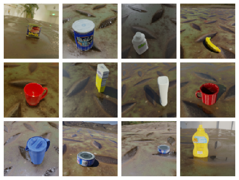
(a) Example images from the YCB-Objects in-distribution test set. Each object is rendered on a background whose texture has similar material properties.

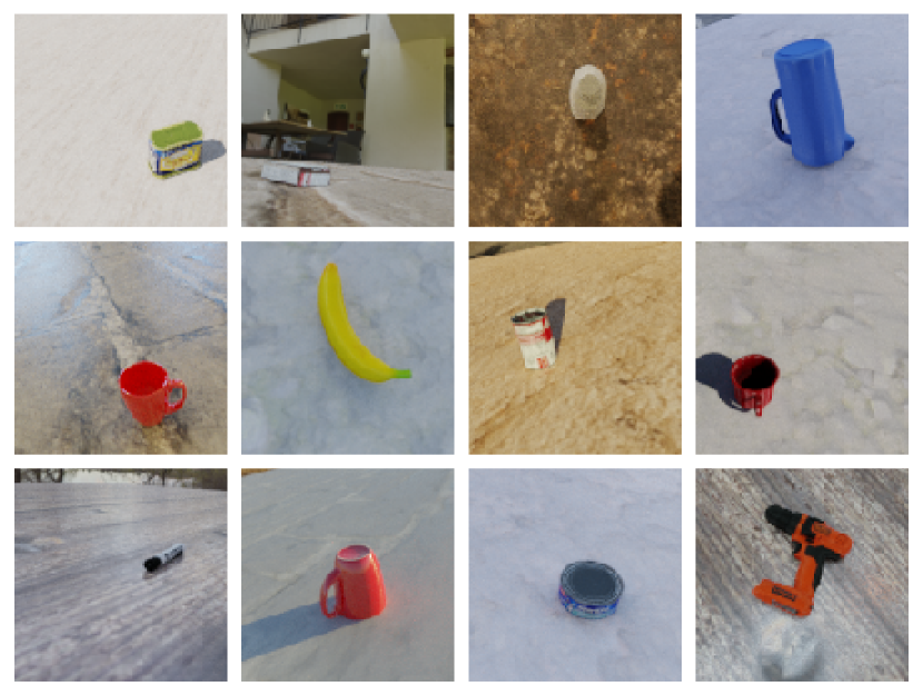
(b) Example images from the YCB-Objects out-of-distribution test set. The distribution shift corresponds to rendering objects on a held out set of textures with a different set of material properties than the in-distribution textures. Aside from the texture change, the set of objects, the lighting environments, and the sampling distribution for objects, poses, and lighting is held fixed between datasets.

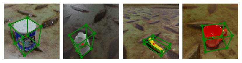
(c) Examples images from the YCB-Objects in-distribution test set shown with keypoint annotations. Each image is annotated with nine keypoints corresponding to the corners of the 3D bounding box and the object center. Models in the testbed predict these keypoints, and the object’s 6D pose is recovered from keypoints using the PnP algorithm [61].

Figure 13: Examples images and keypoint annotations from the YCB-Objects in-distribution and out-of-distribution (texture shift) datasets.

In our datasets, each object is placed on a plane with one of 60 textures from texturehaven.com and rendered with lighting from one of 60 HDRIs from hdrihaven.com. To generate distribution shift, we separate the textures into two, non-overlapping subsets based on their material properties. The in-distribution test set uses one subset of textures, and the out-of-distribution test set uses the other. See Figure 13 for example images corresponding to the in and out-of-distribution textures and corresponding datasets.

We generate datasets by uniformly sampling an object, a background lighting environment, a background texture (from the in or out-of-distribution subset), an object pose, and a camera pose. We generate in-distribution training sets of 50,000 and 100,000 images and both in and out-of-distribution test sets of 10,000 images. In this section, we use the 50,000 example training set for our experiments. We use the 100,000 example training set to explore the effect of adding more i.i.d. training set in Appendix B.2.

In simulation, the object model, the object pose, and the camera pose are all known in advance, so we can easily compute a ground truth pose for each object relative to the scene. We additionally annotate each image in our dataset with 9 2D keypoints corresponding to projection of the 3D bounding box and the 3D center of the object onto the 2D image. Figure 13 visualizes these annotations for a random sample of images from the training set.

A.3.3 YCB-Objects Models

The neural pose estimation models in our testbed are all based on semantic segmentation networks for predicting 2D keypoints. In essence, each network takes as input the entire image of the scene and predicts the nine keypoints previously described and shown in Figure 13. Some implementations in the literature first estimate bounding boxes of the objects in the scene before passing the images to the keypoint prediction network. Since our scenes only contain a single object, the networks in our testbed do not perform this step.

Given 2D keypoints predictions, each model then uses the PnP algorithm [61] to recover the 3D object pose. This approach, developed by Rad and Lepetit [79] and Pavlakos et al. [75] is also used in high-performing implementations like Tremblay et al. [109]. Our testbed contains several models for the semantic segmentation backbone. Unless otherwise noted, the implementation is taken from https://github.com/qubvel/segmentation_models.pytorch.

1. UNet [89] with ResNet [44], MobileNet [91], and EfficientNet-b7 [103] as the encoder.

2. UNet++ [120].

3. FCN_ResNet with varing depths 18, 34, 50, and 101 [65], using the implementation from https://github.com/pytorch/vision/tree/master/torchvision/models/segmentation.

4. LinkNet [20].

5. PSPNet [118].

6. PoseNet [54].

7. 2-layer CNN

Each of these models outputs a set of nine heatmaps, one corresponding to each keypoint prediction. For each model, we use the PnP implementation from Bradski [13].

Appendix B The linear trend phenomenon

In this section, we present additional examples of linear trends between in-distribution and out-of-distribution performance across each of the testbeds discussed in Appendix A. In Appendix B.1, we first highlight examples of linear trends across a variety of distribution shifts for models in each of the CIFAR-10, FMoW-WILDS, ImageNet, and the YCB-Objects “universes” discussed previously. Then, in Appendix B.2, we show these linear trends are invariant to changes in model hyperparameters, training duration, and training set size.

B.1 Further examples of linear trends

B.1.1 CIFAR-10

Dataset reproduction shifts.

In Figure 7, we plot out-of-distribution test accuracy vs. in-distribution CIFAR-10 test accuracy for each of the CIFAR-10 testbed models described in Appendix A.1.5 on two different dataset reproduction shifts: CIFAR-10.1, CIFAR-10.2. For each shift, the relationship between in-distribution and out-of-distribution test accuracy for both classical and neural models is well captured by a linear fit, and the corresponding $R^{2}$ statistic is greater than $0.99$ for each example.

Distribution shifts between machine learning benchmarks.

In Figure 7, we also plot out-of-distribution test accuracy vs. in-distribution CIFAR-10 test accuracy for each of the CIFAR-10 testbed models described in Appendix A.1.5 on two different machine learning benchmark shifts: CINIC-10, and STL-10. The class structure of STL-10 differs slightly from CIFAR-10 and includes a monkey class instead of a frog class. For the STL-10 experiment we therefore consider nine-class variants of STL-10 and CIFAR-10, omitting instances with monkey or frog labels, and, for each model, we mask the frog class (or logit) and predict only among the remaining nine classes. The relationship between ID and OOD accuracy is well-captured by a linear fit and the $R^{2}$ statistic is greater than $0.99$ in each case.

Synthetic perturbations.

In Figure 8, we plot out-of-distribution test accuracy vs. in-distribution CIFAR-10 test accuracy for the same collection of CIFAR-10 testbed models on a subset of eight different synthetic dataset shifts from CIFAR-10-C [46] where very clean linear trends occur— fog, brightness, snow, defocus blur, spatter, elastic transform, frost, and saturate. For each shift, the linear fit well-approximates the relationship between in-distribution and out-of-distribution accuracy, and the $R^{2}$ statistic is greater than $0.94$ for each example. However, the fits are not as clean as the machine learning benchmark shifts discussed previously, and, moreover, for several of the synthetic perturbations in CIFAR-10-C, there is no linear trend at all. We discuss examples from CIFAR-10-C where linear trends fail to hold further in Section 4 and Appendix C.

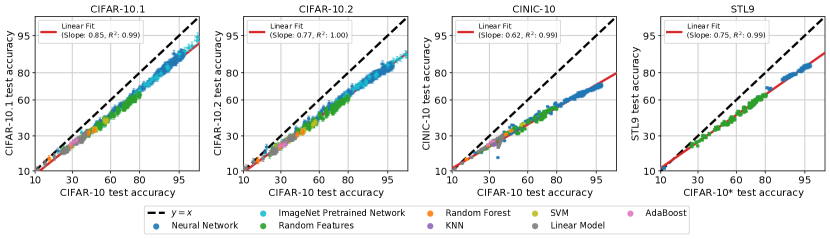
Figure 7: Out-of-distribution accuracies vs. in-distribution CIFAR-10 test accuracies for a wide range of models across two different dataset reproduction shifts, CIFAR-10.1 and CIFAR-10.2, as well as two different shifts between machine learning benchmarks, CINIC-10, and STL-10. Each point corresponds to a model evaluation, shown with 95% Clopper-Pearson confidence intervals (mostly covered by the point markers). For the STL-10 experiment, we consider nine-class subsets of both STL-10 and CIFAR-10, omitting the monkey and frog class, respectively, and restrict each model to predict only from the remaining nine-classes.

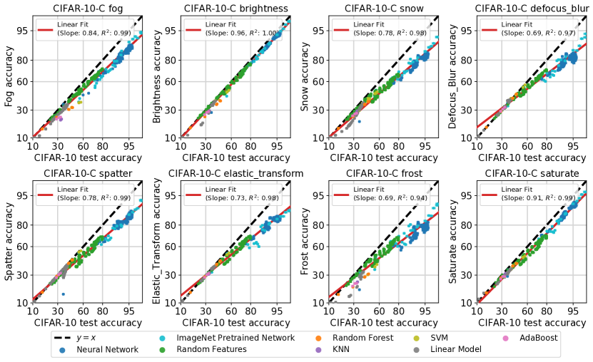
Figure 8: Out-of-distribution accuracies vs. in-distribution CIFAR-10 test accuracies for a wide range of models from our CIFAR-10 testbed across eight synthetic perturbation shifts from CIFAR-10-C. Each point corresponds to a model evaluation, shown with 95% Clopper-Pearson confidence intervals (mostly covered by the point markers).

B.1.2 FMoW-WILDS

In Figure 9, we plot out-of-distribution test accuracy vs. in-distribution FMoW-WILDS test accuracy for both the classical methods and the ImageNet networks from the main testbed described in Appendix A. We evaluate each model on both the out-of-distribution validation and the out-of-distribution test set from FMoW-WILDS using two metrics: average accuracy and worst accuracy over five geographical regions (for more details on FMoW-WILDS, see Appendix A). To remove noise from very low accuracy models, we restrict our attention to models with FMoW-WILDS test set accuracy at least 10%. Across both out-of-distribution datasets and both metrics, the linear fit well-captures the relationship between in and out-of-distribution performance with an $R^{2}$ statistic of a least $0.98$.

Experimental details.

Below, we provide additional technical details about our FMoW-WILDS experiments.

• Datasets. We train each model on the training split of the FMoW-WILDS dataset [25] defined by Koh et al. [55], and perform testing on the in-distribution (ID) and out-of-distribution (OOD) validation and test splits defined by Koh et al. [55].

• Worst-region accuracy confidence intervals. We heuristically obtain confidence intervals for the worst-region accuracy by computing standard 95% Clopper-Pearson confidence intervals for accuracy in the region with the lowest accuracy on the test set for each model.

• Training hyperparameters. Unless otherwise noted, we train all of the neural models using learning rate $10^{-4}$ and weight decay $0$ for 50 epochs. We use Adam throughout with all other parameters set to their default PyTorch values.

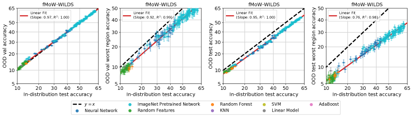
Figure 9: Out-of-distribution accuracies vs. in-distribution FMoW-WILDS test accuracies for a wide range of classical methods and ImageNet networks from our main testbed. Each point corresponds to a model evaluation, shown with 95% Clopper-Pearson confidence intervals (mostly covered by the point markers). Left: In the left two plots, we evaluate each model on the FMoW-WILDS OOD validation set using both average and worst-region accuracy. Right: In the right two plots, we evaluate each model on the FMoW-WILDS OOD test set using both average and worst-region accuracy. In all four cases, a linear fit well captures the relationship between in-distribution and out-of-distribution performance with $R^{2}$ statistics greater than $0.98$ in each setting.

B.1.3 ImageNet

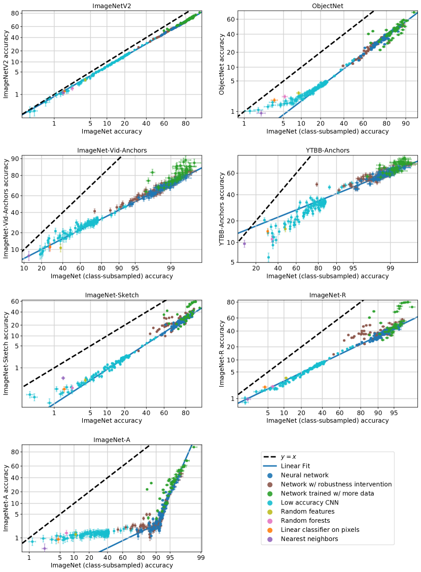
Figure 10: Model accuracies on the ImageNet natural distribution shifts [104]: ImageNetV2, ObjectNet, ImageNet-Vid-Anchors, YTBB-Anchors, ImageNet-Sketch, ImageNet-R, and ImageNet-A. Each point corresponds to a model evaluation, shown with 95% Clopper-Pearson confidence intervals. The axes are scaled via logit scaling, and the linear fit is fit only to standard networks following [104].

In Figure 10, we plot the existing models from Taori et al. [104] alongside the new models in our testbed (CLIP, self-supervised models, and classical methods like random features, random forests, nearest neighbors, and linear regression) on the ImageNet natural distribution shifts. First, we observe that the two CLIP models are significantly robust on all shifts (these models are the two green points above the line at around 60% ImageNet accuracy). This is interesting and is in line with our conclusions that pretraining on extra data can increase model robustness to distribution shift. Second, we observe that all three low-accuracy models lie relatively near the predicted fit line for ImageNetV2, ImageNet-Vid-Anchors, ImageNet-Sketch, and ImageNet-R. Note that this line is fit only to the standard neural networks (blue points). Understanding why the fit isn’t as predictive in the low-accuracy regime for ObjectNet, YTBB-Anchors, and ImageNet-A is an interesting direction for future work. Note that the fit to ImageNet-A is performed piecewise around the ResNet-50 model accuracy following the procedure in Taori et al. [104].

B.1.4 iWildCam-WILDS

Experiment details.

The models reported in the iWildCam-WILDS panel of Figure 1 were obtained using the following parameters. We trained 10 neural network architectures on the iWildCam-WILDS training set (see legend of Figure 11 below). For each architecture, we perform both training from scratch and fine-tuning from a model pretrained on ImageNet. The fine-tuning configurations are similar to the setting of Koh et al. [55]: we train for 12 epochs with batch size 16 using Adam and sweep over learning rate and weight decay values in the grid $\{3\cdot 10^{-5},10^{-4},10^{-3},10^{-2}\}\times\{0,10^{-3},10^{-2}\}$. The other Adam parameters were set to the Pytorch defaults. For models trained from scratch we use the same hyperparameter grid except we train for 15 epochs, which seems to suffice for convergence for each model with at least some of the learning rates. For details on error bar calculation and label noise reduction, see Appendix A.1.4.

Architecture variation with fixed weight decay.

Figure 11 provides a more detailed view of the iWildCam-WILDS experiments, wherein we plot the final epoch performance of the models we train, where the weight decay is set to zero. As the figure shows, the error bars for all model intersect the fitted linear trend line (in probit domain), with the exception of AlexNet when training from scratch, which is slightly below the linear trend. Varying the weight decay parameter appears to affect the ID/OOD trend of fine-tuned model; see Section 5 and Appendix D.3 for additional discussion and plots.

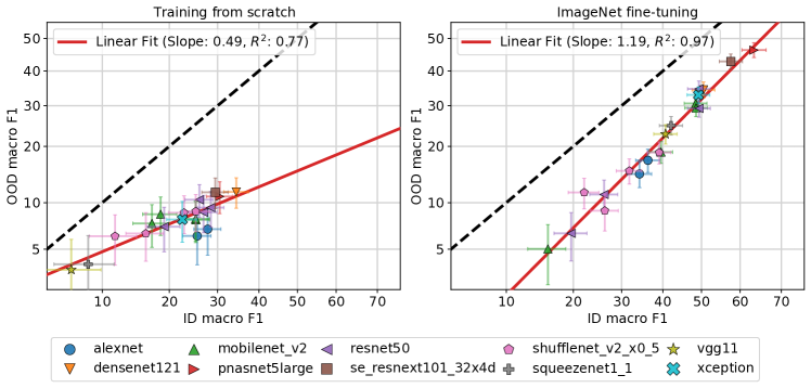
Figure 11: OOD vs. ID macro F1 scores for iWildCam-WILDS models trained from scratch (left) or fine-tuned from pretrained ImageNet models (right), with varying model architecture and learning rate, but weight decay fixed to zero. Contrast with Figure 32 for results when varying the weight decay parameter.

B.1.5 YCB-Objects

In Figure 12, we plot out-of-distribution accuracy versus in-distribution accuracy for a synthetic 6D pose estimation task using the YCB object models from Calli et al. [17] and a testbed of neural models for 6D pose estimation. As in the previous examples, a linear fit well-approximates the relationship between in and out-of-distribution accuracy with an $R^{2}$ statistic of $0.99$.

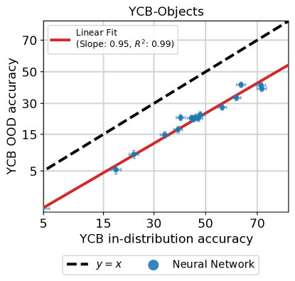
Figure 12: Out-of-distribution accuracy vs. in-distribution accuracy for a synthetic 6D pose estimation task based on the YCB object models from Calli et al. [17] across a testbed of neural pose estimation networks. Each point corresponds to a model evaluation shown with 95% Clopper-Pearson confidence intervals. The distribution shift corresponds to varying the background texture for rendered images of the YCB objects. See Figure 13 for example images both in and out-of-distribution. Appendix B.1.5 describes the dataset and the model testbed in more detail.

Experimental details.

We train two variants of each model. The first variant is trained with standard $\ell_{2}$ loss on the distance between the predicted heatmap and the ground truth keypoint location (with a Gaussian blur of $\sigma=0.2$). These models predict keypoint locations by taking an $\arg\max$ over the heatmap. The other variant is trained with and makes predictions using the integral pose regression technique of [98]. We train each model using SGD with momentum and learning rate annealing. For each model, we optimized the learning rate in $[10^{-4},10^{-1}]$ and weight decay in $[10^{-4},1]$.

B.2 Variations in model hyperparameters, training duration, and training dataset size

In this section, we explore the sensitivity of the linear trends discussed in Appendix B.1 to variation in model hyperparameters, training duration, and training set size.

We focus much of our exploration on two datasets CIFAR-10 and FMoW-WILDS. We selected CIFAR-10 for ease of experimentation, and we selected FMoW-WILDS in order to understand the sensitivity of the linear trends outside the context of machine learning benchmark or synthetic shifts.

B.2.1 CIFAR-10

In Figures 14, 15, and 16, we probe the sensitivity of the linear trend between in and out-of-distribution test accuracy for CIFAR-10 models to three types of variation: variation in hyperparameters, variation in training duration, and variation in training set size. For ease of visualization, we focus our experiments on three model families spanning low, moderate, and high accuracy regimes: a ridge regression classifier on image pixels, the random feature model from Coates et al. [27], and a ResNet [45]. The results are virtually identical, but harder to visualize, when considering a larger number of model families simultaneously.

We systematically vary the hyperparameters, number of training epochs (for the ResNets), and the size of the training set for models from each class. We plot model evaluations on the same linear trend line as found in Appendix B.1. We show variation along these three dimensions moves models along the linear trend line for each dataset, but does not change the linear fit. For each of the dataset reproduction shift CIFAR-10.2 (Figure 14), the benchmark shift CINIC-10 (Figure 15), and the synthetic CIFAR-10-C fog shift (Figure 16), the $R^{2}$ statistic of the fit is greater than $0.99$.

Experimental details.

We briefly provide details about the specific variations we consider for each model class.

1. Hyperparameter variation: For the ridge regression classifier, we vary the $\ell_{2}$ regularization parameter in $[10^{-6},10^{10}]$. For the random features models, we vary the $\ell_{2}$ regularization parameter in $[10^{-4},10^{6}]$ and the number of random features in $[2^{0},2^{14}]$. For the ResNet model, we vary network depth in $\{18,34,50,101\}$, learning rate in $[10^{-5},10]$, momentum in $[0.33,0.99]$, and weight decay in $[10^{-5},10^{5}]$.

2. Training duration variation: To understand sensitivity to training duration, we save and evaluate each ResNet model after every epoch of training. We train each model for 350 epochs, giving 350 evaluations per run.

3. Training set size variation: To understand sensitivity to the amount of training data, we subsample the CIFAR-10 dataset from the original 50,000 samples to i.i.d. class-balanced subsets of size 1000, 5000, 10000, 15000, 25000, and 40000 examples. We train each of the hyperparameter configurations for each model class on each of the 6 subsets of the original dataset and evaluate them on the same in and out-of-distribution test sets as before.

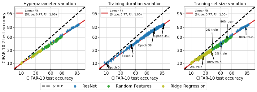
Figure 14: Out-of-distribution CIFAR-10.2 accuracies vs. in-distribution CIFAR-10 test accuracies under variations in model hyperparameters, training duration, and the size of the training set. Each point corresponds to a model evaluation, shown with 95% Clopper-Pearson confidence intervals (mostly covered by the point markers). In each panel, we compare models with the linear trend line from Appendix B.1. Left: For each model family, we vary model-size, regularization, and optimization hyperparameters. Middle: We evaluate each network after every epoch of training. Right: We train models on randomly sampled subsets of the training data, ranging from 2% to 80% of the original CIFAR-10 training set size. In each setting, variation in hyperparameters, training duration, or training set size moves models along the trend line, but does not affect the linear fit.

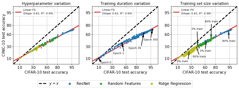
Figure 15: Out-of-distribution CINIC-10 accuracies vs. in-distribution CIFAR-10 test accuracies under variations in model hyperparameters, training duration, and the size of the training set. Each point corresponds to a model evaluation, shown with 95% Clopper-Pearson confidence intervals (mostly covered by the point markers). In each panel, we compare models with the linear trend line from Appendix B.1. Left: For each model family, we vary model-size, regularization, and optimization hyperparameters. Middle: We evaluate each network after every epoch of training. Right: We train models on randomly sampled subsets of the training data, ranging from 2% to 80% of the original CIFAR-10 training set size. In each setting, variation in hyperparameters, training duration, or training set size moves models along the trend line, but does not affect the linear fit.

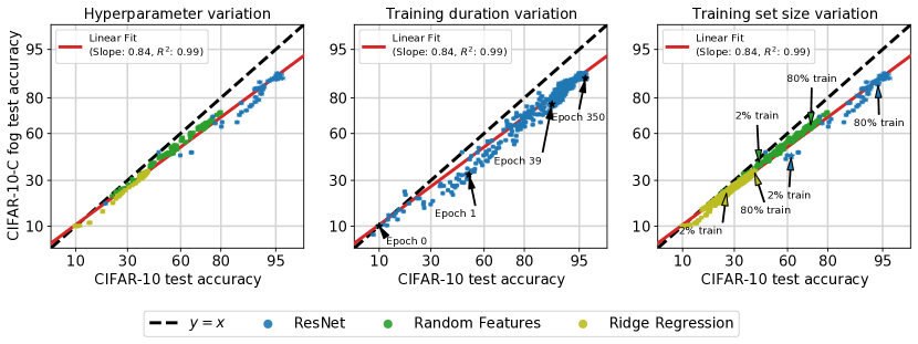
Figure 16: Out-of-distribution CIFAR-10-C fog accuracies vs. in-distribution CIFAR-10 test accuracies under variations in model hyperparameters, training duration, and the size of the training set. Each point corresponds to a model evaluation, shown with 95% Clopper-Pearson confidence intervals (mostly covered by the point markers). In each panel, we compare models with the linear trend line from Appendix B.1. Left: For each model family, we vary model-size, regularization, and optimization hyperparameters. Middle: We evaluate each network after every epoch of training. Right: We train models on randomly sampled subsets of the training data, ranging from 2% to 80% of the original CIFAR-10 training set size. In each setting, variation in hyperparameters, training duration, or training set size moves models along the trend line, but does not affect the linear fit.

B.2.2 FMoW-WILDS

As in the previous section, in Figure 17, we probe the sensitivity of the linear trend for FMoW-WILDS models to variation in hyperparameters, variation in training duration, and variation in training set size. For ease of visualization, we focus our experiments on three model families spanning low, moderate, and high accuracy regimes: a random forest model on image pixels, the random feature model from Coates et al. [27], and a ResNet [45]. We plot model evaluations on the same linear trend line as found in Appendix B.1. We show variation along these three dimensions moves models along the linear trend line for each dataset, but does not change the linear fit: the $R^{2}$ statistic of the fit is greater than $0.99$ for every setting under the accuracy metric and greater than $0.91$ for the worst-region accuracy metric.

Experimental details.

We briefly provide details about the specific variations we consider for each model class.

1. Hyperparameter variation: For the random forest classifier, we vary the maximum depth in $\{1,3,10,20\}$, the number of trees in $\{10,20,50,200\}$, and the splitting criterion between entropy and gini impurity. For the random features models, we vary the $\ell_{2}$ regularization parameter in $[10^{-4},10^{6}]$ and the number of random features in $[2^{0},2^{8}]$. For the ResNet model, we vary network depth in $\{18,34,50,101\}$, learning rate in $[10^{-5},10]$, momentum in $[0.33,0.99]$, and weight decay in $[10^{-5},10^{5}]$.

2. Training duration variation. We train each configuration of the ResNet for 70 epochs and evaluate each model after every epoch of training.

3. Training set size variation. We i.i.d. subsample the FMoW-WILDS train dataset from the original 76,863 examples to subsets of size 1000, 5000, 10000, 20000, and 50000 examples. We train each of the hyperparameter configurations for each model class on each of the 5 subsets of the original dataset and evaluate them on the same in and out-of-distribution test sets as before.

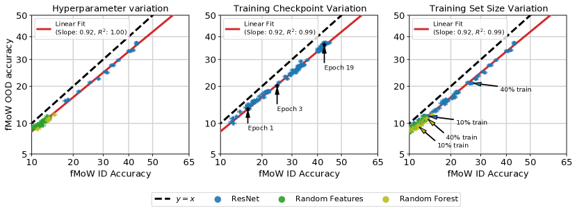
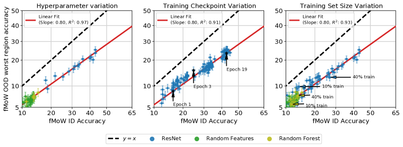
Figure 17: Out-of-distribution FMoW-WILDS test accuracies vs. in-distribution FMoW-WILDS test accuracies under variations in model hyperparameters, training duration, and the size of the training set. Each point corresponds to a model evaluation, shown with 95% Clopper-Pearson confidence intervals. In each panel, we compare models with the linear trend line from Appendix B.1. The top row compares model trends using average accuracy as the OOD metric, and the bottom rows uses worst-region accuracy as the OOD metric. Left: For each model family, we vary model-size, regularization, and optimization hyperparameters. Middle: We evaluate each network after every epoch of training. Right: We train models on randomly sampled subsets of the training data, ranging from 2% to 80% of the original CIFAR-10 training set size. In each setting, variation in hyperparameters, training duration, or training set size moves models along the trend line, but does not affect the linear fit.

B.2.3 YCB-Objects

In Figure 18, we see that the linear fit for the YCB-Objects experiment from Appendix B.1.5 is also invariant to changes in the amount of training data.

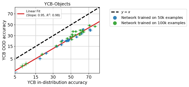
Figure 18: Out-of-distribution YCB-Objects test accuracies vs. in-distribution YCB-Objects test accuracies under variations in training set size. Each point corresponds to a model evaluation, shown with 95% Clopper-Pearson confidence intervals. The linear trend line is the same as Figure 12. The linear trend still well explains the data ($R^{2}=0.98$), and increasing training set size moves models along the linear trend, but does not affect the linear fit.

B.3 Comparison of axis scaling

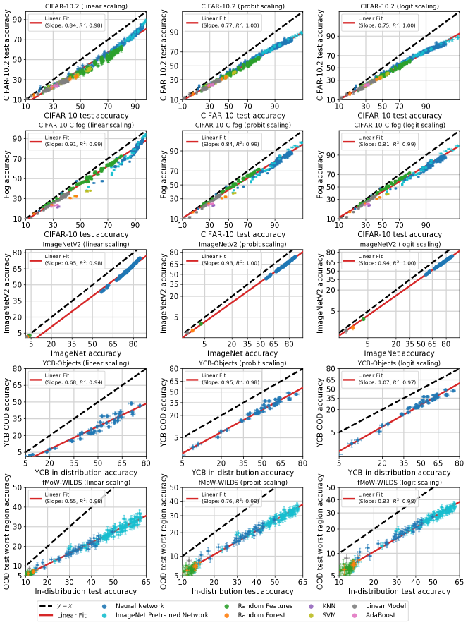
Figure 19: OOD test accuracies vs. ID test accuracies for several pairs of ID and OOD test sets visualized with three different axis scalings. Left: The left column shows model accuracies with a linear axis scaling. Middle: The middle column shows model accuracies with a probit scale on both axes. In other words, model accuracy $x$ appears at $\Phi^{-1}(x)$ where $\Phi^{-1}$ is the inverse Gaussian CDF. Right: The right column shows model accuracies with a logit scale on both axes: model accuracy $x$ appears at $\sigma^{-1}(x)$ where $\sigma^{-1}$ is the inverse logistic function. Visual inspection shows the linear fit is better in the logit or probit domain, especially when model accuracies span a wide range. Quantitatively, the R2 statistics are higher in the probit or logit domains than with linear axis scaling. For instance, on ImageNetV2 and CIFAR-10.2, the $R^{2}$ is $0.98$ in the linear domain compared to $1.0$ in the probit or logit domains.

Appendix C Distribution shifts with weaker correlations

C.1 Camelyon17-WILDS

In this section, we first explore the role of training randomness on the observed ID-OOD correlation for Camelyon17-WILDS. Remember that in Figure 3, we found a very high degree of variability between ID and OOD performance. To see if the performance variation was due to training randomness, we train each model ten times and then average the final model accuracies together. The result of these averaged runs is displayed in Figure 20 (left). The $R^{2}$ value for the averaged runs comes in at $R^{2}=0.39$, which is approximately equivalent to the $R^{2}$ value in Figure 3 ($R^{2}=0.40$); this suggests that training randomness is not enough to account for the performance variability.

In Figure 20 (right), we also attempted early-stopping each trained model on a separate OOD validation set (different in distribution from the OOD test set), as is recommended in [55], before averaging model accuracies; the result is largely unchanged and comes in at $R^{2}=0.46$. Early-stopping on the in-distribution validation set, however, does increase ID-OOD correlation significantly to $R^{2}=0.77$, as seen in Figure 20 (middle); further investigating the mechanisms at play here is an interesting direction for future work.

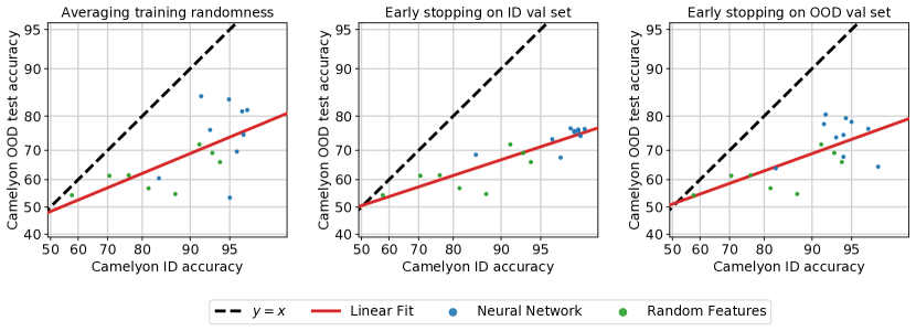
Figure 20: Model accuracies on the Camelyon17-WILDS distribution shift. Each point gives average accuracies for models trained with ten different random seeds, and error bars give the standard deviation. Left: Models trained to convergence and then averaged over seeds. Middle: Each model is early-stopped on the ID validation set then averaged over seeds. Right: Each model is early-stopped on the OOD validation set then averaged over seeds.

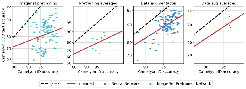
Figure 21: Model accuracies on the Camelyon17-WILDS distribution shift. Left: ImageNet pretrained models finetuned to convergence. Middle Left: ImageNet pretrained model accuracies averaged over ten random seeds. Middle Right: Models trained with targeted color jitter data augmentation. Right: Data augmentation model accuracies averaged over ten random seeds.

As a next step, to study the role of the training data distribution on the observed trends, we conduct two specific training-time interventions: pretraining on ImageNet, and training using a specific color-jitter data augmentation.

We show results for models pretrained on ImageNet in Figure 21 (left). As is evident, the variability in model performance is still extremely high ($R^{2}=0.05$). Averaging over training randomness does not seem to help either ($R^{2}=0.14$).

We also train using a domain-specific color-jitter data augmentation designed to mimic the visual differences in samples from different hospitals, a technique that has previously been found to have been beneficial on a similar task [105, 106]. As seen in Figure 21 (middle right), training with the data augmentation both considerably increases average OOD performance and significantly reduces the amount of OOD accuracy variation ($R^{2}=0.77$). However, even with the targeted data augmentation, large OOD accuracy fluctuations still exist. Averaging over training randomness greatly increases the correlation further and mitigates these fluctuations ($R^{2}=0.95$), as seen in Figure 21 (right); however, the data augmentation causes all models to have relatively high ID accuracy, and it is unclear whether this tight trend would hold for models in the low accuracy regime as well.

One possible reason for the high variation in accuracy is the correlation across image patches. Image patches extracted from the same slides and hospitals are correlated because patches from the same slide are from the same lymph node section, and patches from the same hospital were processed with the same staining and imaging protocol. In addition, patches in Camelyon17-WILDS are extracted from a relatively small number of slides (the dataset includes 50 slides total, and there are 10 slides from a single hospital in the OOD test set [55]). Prior work in the context of natural language processing tasks have shown that these correlations can result in instabilities in both training and evaluation [119], and investigating their effect on OOD variation in Camelyon17-WILDS is interesting future work.

As an initial exploration of the effect of highly correlated test examples, we observe that correlated examples can result in high OOD variation in a simulated environment on CIFAR-10 and CIFAR-10.2. Concretely, we subsample CIFAR-10 and CIFAR-10.2 and then apply data augmentation to each example to generate a test set of the same size as the original but with significant correlation between examples. In each panel in Figure 22, we train models on CIFAR-10 and then evaluate them on CIFAR-10 and CIFAR-10.2 with effective test size $k$ for varying $k$. Concretely, we subsample $k$ images from each class, and then apply RandAugment rand-m9-mstd0.5-inc1 [29] to each example to generate test sets of size 10,000. We work with a binary version of CIFAR-10 and CIFAR-10.2, restricting both datasets to two classes: airplanes and cats. When the effective test set size is small, e.g. $k=1$ or $k=2$, the linear fit is very poor. However, as the effective test set size $k$ increases to $k=100$ or $k=500$, the linear fit is much better ($R^{2}=0.94$ vs. $R^{2}=0.66$), and the variance between model evaluations is substantially smaller.

In contrast to highly correlated test examples, highly correlated training examples appears to have substantially less effect on the amount of OOD variation or the quality of the linear fit. Using the same simulated CIFAR-10 and CIFAR-10.2 environment as the previous paragraph, we generate a sequence of training sets with varying degrees of correlation between training examples. Concretely, we subsample the CIFAR-10 and CIFAR-10.2 training sets and then apply data augmentation (RandAugment [29]) to each example to generate a training set of the same size as the original but with significant correlation between examples. In each panel in Figure 23, we train models on CIFAR-10 and then evaluate them on CIFAR-10. Even with the effective training set size is small, e.g. $k=2$, the linear fit is fairly good ($R^{2}=0.89$), and there is substantially smaller variance between model evaluations than in the corresponding effective test-size experiment.

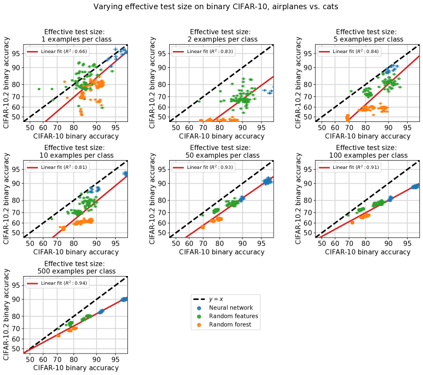
Figure 22: Models trained on CIFAR-10 and evaluated on CIFAR-10.2 for binary classification: airplanes vs cats. Each panel depicts evaluating the models with varying effective test set sizes $k$, where $k$ images are subsampled from each class and then repeated data-augmented using RandAugment [29] to generate a consistent test set size of 10,000 examples. For smaller effective test set sizes, the linear fit is very poor, and this variance decreases substantially for larger $k$.

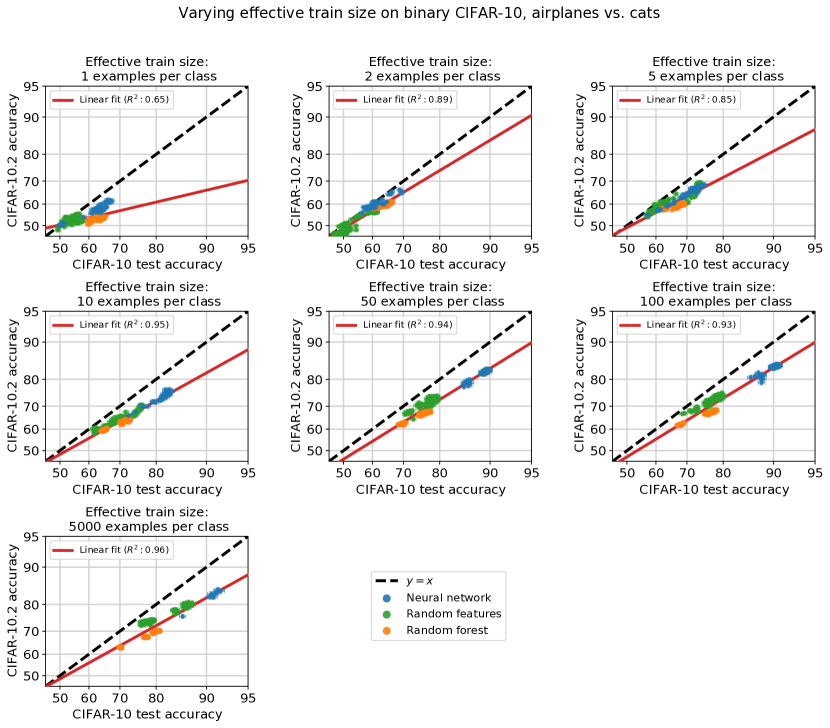
Figure 23: Models trained on CIFAR-10 and evaluated on CIFAR-10.2 for binary classification: airplanes vs cats. Each panel depicts evaluating the models with varying effective train set sizes $k$, where $k$ images are subsampled from each class and then repeatedly data-augmented using RandAugment [29] to generate a consistent train set size of 50,000 examples. In contrast to varying the effective test set size (see Figure 23), varying the effective train set has little effect on the quality of the linear fit. For instance, with as few as two effective examples per class, the linear fit is fairly precise ($R^{2}=0.89$).

C.2 CIFAR-10-C

In this section, we look at distribution shifts induced by image corruptions in more detail. Specifically, in Figures 24–28, we plot neural networks trained on either CIFAR-10 or ImageNet and evaluated on a similar set of image corruptions. Interestingly, the choice of corruption can have a significant effect on the strength of the linear trend between ID and OOD accuracy, as we have already explored in Sections 3 and 4. Comparing the plots in Figures 24–28 side-by-side, we also observe that many corruptions behave more linearly on ImageNet-C than on CIFAR-10-C. Investigating this discrepancy further is an interesting direction for future work.

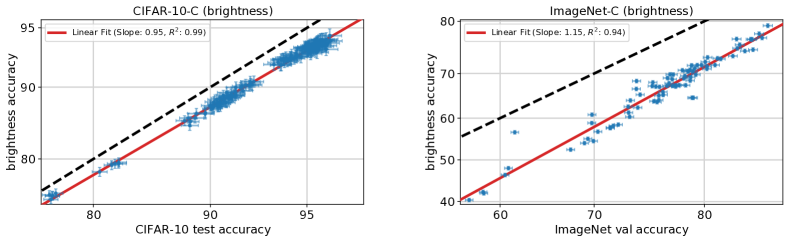
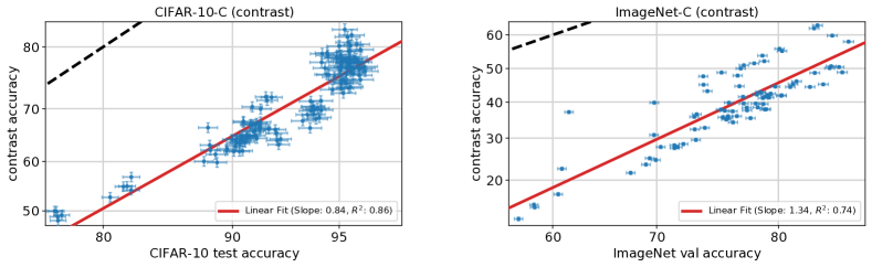
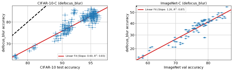
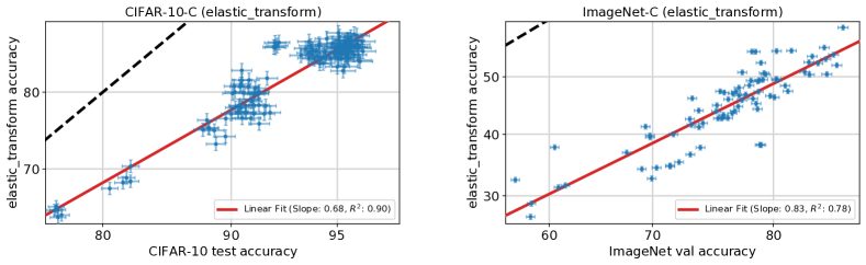
Figure 24: Models trained on either CIFAR-10 (left) or ImageNet (right) and evaluated under distribution shift due to image corruptions. This figure continues for the next few pages.

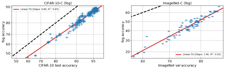
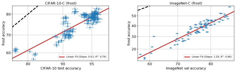
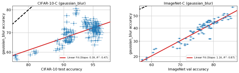
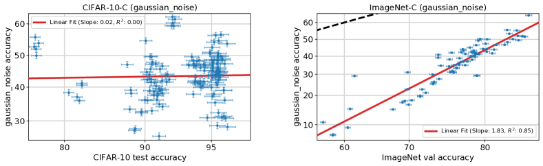
Figure 25: Continuation of the corruption plots.

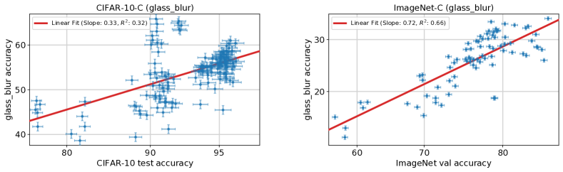
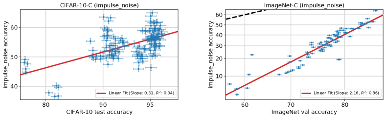
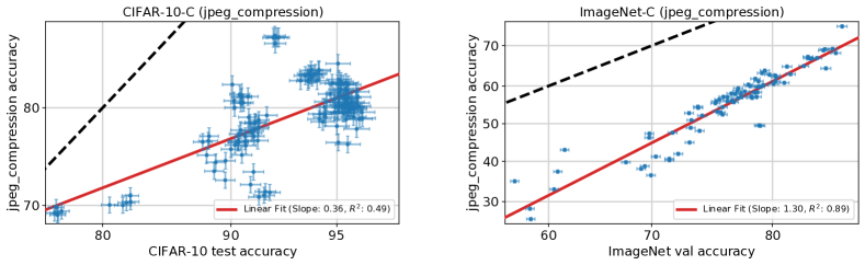
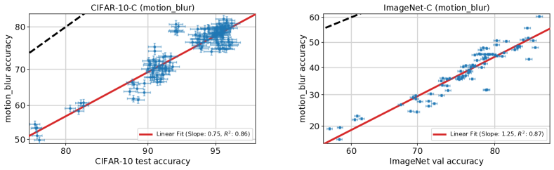
Figure 26: Continuation of the corruption plots.

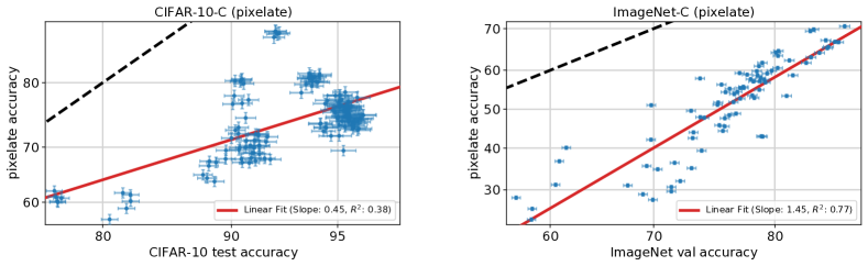
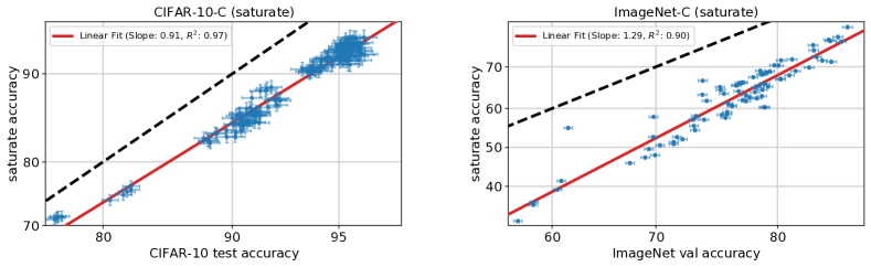
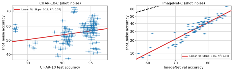
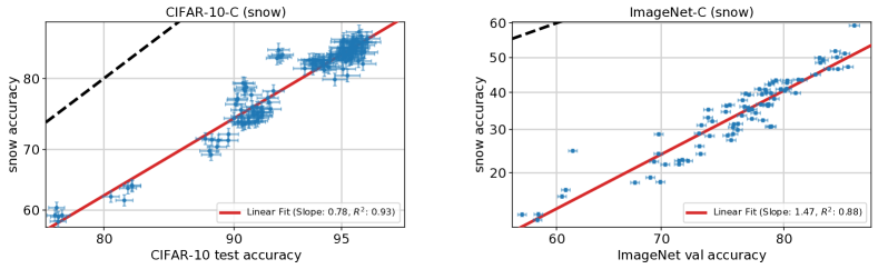
Figure 27: Continuation of the corruption plots.

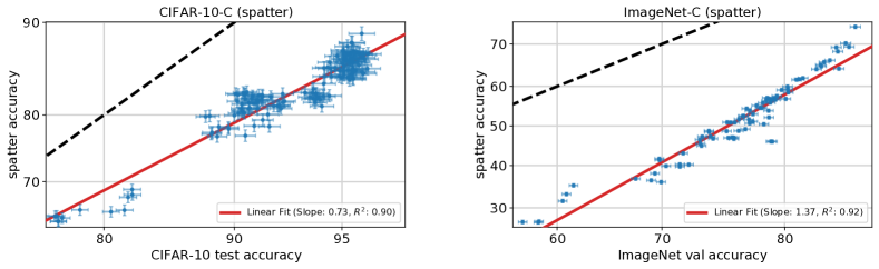
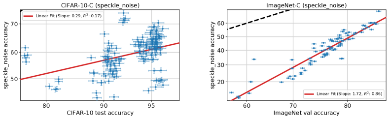
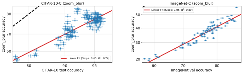
Figure 28: Continuation of the corruption plots.

C.3 iWildCam-WILDS-v1.0

We now study version 1.0 of iWildCam-WILDS (from WILDS version 1.0), which has a different split between training and ID test sets, compared to the version of iWildCam-WILDS we have studied thus far (iWildCam-WILDS version 2.0 from WILDS version 1.1). In version 1.0, images from training cameras are assigned uniformly at random between the train and ID test sets, whereas images are randomly partitioned by date between train and ID test splits in version 2.0. Since the images tend to be taken in bursts, the earlier version of the dataset contains some training and ID test examples that are taken within the same image sequence, and these images tend to be similar because they often capture the same animal at the same location. In other words, we are changing how we measure in-distribution performance, and in this way, our investigation on ID/OOD correlations study different distribution shifts between the two versions. Nevertheless, both versions of the dataset measure out-of-distribution performance in the same way, with train and OOD test splits containing images from disjoint cameras.

While we use version 2.0 in all other sections, it is still interesting to understand how a different in-distribution train-test split affects the ID/OOD correlation. In Figure 29, we repeat the experiment reported in Figure 11 on the v1.0 split. As the figure shows, the ID/OOD correlation is far less pronounced when using the v1.0 split. Moreover, the fine-tuned models show a near-vertical line, with models concentrated around high ID accuracy values but spread across many OOD values, and this could potentially be explained by the high image similarity between train and ID test sets.

Finally, we remark that while the v2.0 split eliminates overlap in image sequence between train and ID test sets, some near-duplicates inevitably persist in that version as well, particularly for empty frames taken during similar times in the day by the same camera. Investigating the effect of this on the linear trend on iWildCam-WILDS v2.0, in which we observe higher variation in performance than in other datasets, is interesting future work.

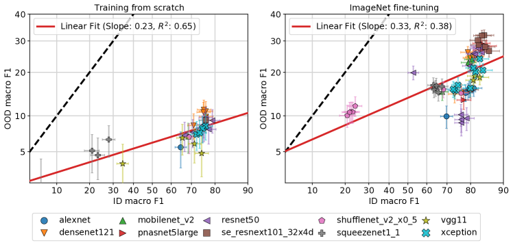
Figure 29: OOD vs. ID macro F1 scores for iWildCam-WILDS-v1.0 models trained from scratch (left) or fine-tuned from pretrained ImageNet models (right), with varying model architecture and learning rate, but weight decay fixed to zero. Contrast with Figure 11 for results on the v2.0 ID test/train split.

Appendix D The effect of pretrained models

D.1 Detailed findings for CIFAR-10

In Figure 30 (left) we reproduce the results shown in Figure 5 and add to it a number of additional models; Figure 30 (right) graphs the performance of the same model when measuring their OOD performance on CIFAR-10.1 instead of CIFAR-10.2. Let us describe the additional models and their relationship to the linear trend.

First, as a middle ground between zero-shot use of ImageNet models (which is above the line) and fine-tuning (which is on the line), we consider neural network models trained only on the subset of CINIC-10 that originates from ImageNet (as opposed to CIFAR-10). It is worth noting that in this case, the CINIC-10 subset includes images from ImageNet-21k, which is a superset of the more common ImageNet-1k dataset containing approximately 21,000 classes. Similar to the zero-shot case, these models use only ImageNet data and so we expect their accuracy to not obey the same CIFAR-10/CIFAR-10.2 relationship of models trained on CIFAR-10 data (in fact, for these models both CIFAR-10 and CIFAR-10.2 are OOD). Similar to fine-tuned models, these models are specialized to the task of classifying only the 10 CIFAR-10 classes (as opposed to the 1000 ImageNet classes), and so we expect them to have better accuracy. Figure 30 lists these models as “Training on ImageNet data,” and confirms our expectations: these models are above the linear fit and have better accuracy than the ImageNet zero-shot models. However, in comparison to the zero-shot models, they appear to lie closer to the linear fit for CIFAR-10-trained models.

Second, we consider two publicly released CLIP models [80], based on ResNet 50 and Vision Transformer, respectively. Both zero-shot application of CLIP and the training of only its final layer (denoted “linear probe”) produce performance that is above the line, particularly for the higher-performing Vision Transformer. See below for additional details on the use of CLIP in our experiments.

Finally, we consider models trained on auxiliary unlabeled data originating from the 80 Million Tiny Images [108], abbreviated 80MTI below, which is a superset of both CIFAR-10 and its reproductions CIFAR-10.1 and CIFAR-10.2. In particular, we consider a model trained via self-training using a subset of TinyImages [18], listed as 80MTI ST in Figure 30), and two models trained via out-distribution aware self-training [2], listed as 80MTI ODST. As the figure shows, despite using auxiliary data, the “80MTI ST” performance is precisely on the CIFAR-10-only linear trend. This might be due to the fact that Carmon et al. [18] filter 80MTI, using a model supervised with the CIFAR-10 training set, thereby possibly losing the additional diversity of TinyImages. The performance of the ODST models appear to deviate from the linear trend. However, the direction of the deviation is inconsistent, being below the line on CIFAR-10.2 and above the line on CIFAR-10.1. Since these are the highest-accuracy models in our testbed it is not completely clear whether these deviations are due to use of extra data or a deviation of the overall ID-OOD trend from a perfect probit linear fit at high accuracies.

Experiment details.

Below we provide some additional details on out CIFAR-10 auxilliary data experiments.

• Zero-shot classification with ImageNet models. To investigate models that are minimally affected by the CIFAR-10 training set, we utilized pre-trained ImageNet models directly for the CIFAR-10 classification task without any fine-tuning (“zero-shot”). A complication here is that the CIFAR-10 classes do not match the ImageNet classes. For instance, ImageNet contains more than 100 different dog classes corresponding to different breeds while CIFAR-10 contains only one dog class. To address this point, we manually constructed a mapping from CIFAR-10 classes to ImageNet classes. Our mapping roughly followed the WordNet hierarchy with some refinements from the class structure used in the human annotation experiments conducted by [95]. We then evaluated the ImageNet models using only the logits for classes appearing in this mapping and picked the CIFAR-10 class as prediction that corresponded to the ImageNet class with the largest logit.

• Zero-shot classification with CLIP models. For the models described as “CLIP zero-shot", we use the publicly released CLIP package, which includes the ResNet and VisionTransformer models as well as the text tokenizer and encoder used to encode the zero-shot text prompts. We obtained the CIFAR-10 prompts through private correspondence with the OpenAI team. For each CIFAR-10 class, we ensembled the prompts by averaging the embeddings of the prompts together before using it for final classification.

• Linear probes. In the models described above as “linear probes” we train only the last layer of a pre-trained neural network by performing (exact) least-squares linear regression of 1-hot class representation using the activations of the network’s penultimate layer.

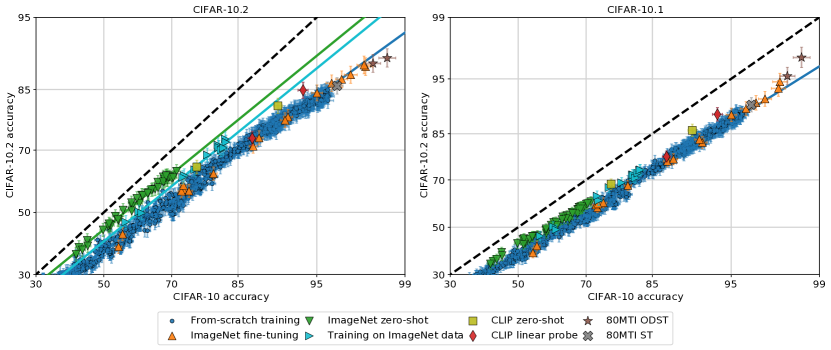
Figure 30: The effect of additional training data on OOD accuracy on CIFAR-10.2 (left) and CIFAR-10.1 (right).

D.2 Detailed findings for FMoW-WILDS

Figure 31 shows a reproductions of Figure 5 (middle) when using different combination of worst-region and average-region accuracy metric for the ID and OOD data (recall that the ID/OOD split is based on time). As the figure shows, the effect of fine-tuning pre-trained models is consistent across the four combinations: fine-tuning improves performance without deviating from the line. We also consider a linear probe of CLIP (see description in the previous subsection). Unlike the result on CIFAR-10, here the CLIP models do not significantly deviate from the linear trend. A possible explanation for this difference is that the web images on which CLIP was trend contain far more images of objects relevant for the CIFAR-10 classification task than they do for the FMoW-WILDS satellite image classification task.

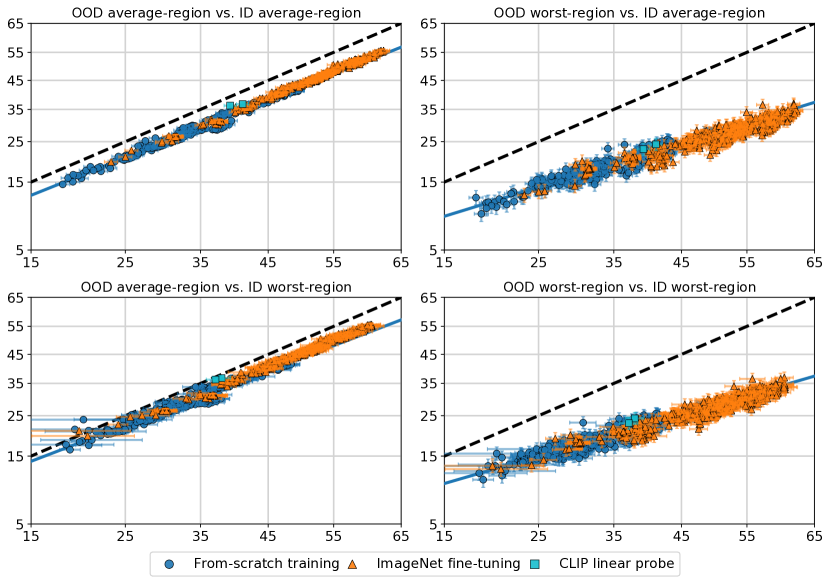
Figure 31: The effect of additional training and different accuracy metrics on FMoW-WILDS ID/OOD performance.

D.3 Detailed findings for iWildCam-WILDS

Figure 32 shows the same models plotted in the iWildCam-WILDS panel of Figure 1, but separating the models trained from scratched and the fine-tuned models, and coloring points by the weight decay parameters. (For each weight decay we vary model architecture and learning rate). For fine-tuned models, there is a clear difference in the ID/OOD linear between model using weight decay 0 and models using nonzero weight decay. In particular, points with nonzero weight decay seem to lie above the zero weight decay linear trend. For models trained from scratch the macro F1 measurement error does not allow us to conclude with confidence whether weight decay affects the linear trend. Finally, it is worth noting that—even though increasing weight decay appears to move models above the zero weight decay line—the models with the best performance, both ID and OOD, do not use weight decay.

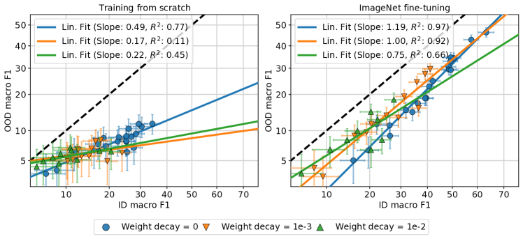
Figure 32: OOD vs. ID macro F1 scores for iWildCam-WILDS models trained from scratch (left) or fine-tuned from pretrained ImageNet models (right), with varying model architecture, learning rates, and weight decay. We observe that fine-tuned models exhibit a different linear trend than models trained from scratch, and moreover that the weight decay parameters affects the ID/OOD correlation, at least for fine-tuned models.

Appendix E Theoretical models for linear fits

E.1 Proof of Theorem 1

See 1

Proof.

We begin by deriving expression for the accuracy of linear classifiers in our Gaussian distributional model. Under distribution $D$, the accuracy of linear classifier $\boldsymbol{\theta}$ is

$$\mathrm{acc}_{D}(\boldsymbol{\theta}) =\Pr\left(\operatorname{\mathrm{sign}}(\boldsymbol{\theta}^{\top}\boldsymbol{x})=y\right)=\Pr\left(y\cdot\boldsymbol{\theta}^{\top}\boldsymbol{x}\geq 0\right)=\Pr\left(\mathcal{N}(\boldsymbol{\theta}^{\top}\boldsymbol{\mu};\|\boldsymbol{\theta}\|^{2}\sigma^{2})\geq 0\right)$$

$$=\Pr\left(\|\boldsymbol{\theta}\|\sigma\cdot\mathcal{N}(0;1)\geq-\boldsymbol{\theta}^{\top}\boldsymbol{\mu}\right)=\Phi\left(\frac{\boldsymbol{\theta}^{\top}\boldsymbol{\mu}}{\|\boldsymbol{\theta}\|\sigma}\right),$$

where we recall that $\Phi(t)=\int_{-t}^{\infty}\frac{1}{\sqrt{2\pi}}e^{-s^{2}/2}\mathrm{d}s=\int_{-\infty}^{t}\frac{1}{\sqrt{2\pi}}e^{-s^{2}/2}\mathrm{d}s$ is the standard Normal cdf. Similarly, for the shifted distribution $D^{\prime}$ we have

$$\mathrm{acc}_{D^{\prime}}(\boldsymbol{\theta})=\Phi\left(\frac{\boldsymbol{\theta}^{\top}\boldsymbol{\mu}^{\prime}}{\|\boldsymbol{\theta}\|\sigma^{\prime}}\right)=\Phi\left(\frac{\alpha}{\gamma}\cdot\frac{\boldsymbol{\theta}^{\top}\boldsymbol{\mu}}{\|\boldsymbol{\theta}\|\sigma}+\frac{\beta}{\gamma\sigma}\cdot\frac{\boldsymbol{\theta}^{\top}\boldsymbol{\Delta}}{\|\boldsymbol{\theta}\|}.\right)$$

Therefore,

$$\left\lvert\Phi^{-1}\left(\mathrm{acc}_{D^{\prime}}(\boldsymbol{\theta})\right)-\frac{\alpha}{\gamma}\Phi^{-1}\left(\mathrm{acc}_{D}(\boldsymbol{\theta})\right)\right\rvert=\frac{\beta}{\gamma\sigma}\left\lvert(\boldsymbol{\theta}/\|\boldsymbol{\theta}\|)^{\top}\boldsymbol{\Delta}\right\rvert.$$ (2)

Since $\boldsymbol{\theta}$ is independent of $\boldsymbol{\Delta}$ and $\boldsymbol{\theta}/\|\boldsymbol{\theta}\|$ is a unit vector, the inner product $(\boldsymbol{\theta}/\|\boldsymbol{\theta}\|)^{\top}\boldsymbol{\Delta}$ is distributed identically to the first coordinate of $\boldsymbol{\Delta}$. A standard concentration bound on the sphere [see, e.g., 3, Lemma 2.2] states that

$$\Pr(\lvert\boldsymbol{\Delta}_{1}\rvert>z)\leq 2e^{-dz^{2}/2}$$

for all $z\geq 0$. Substituting $z=\sqrt{2d^{-1}\log\frac{2}{\delta}}$ completes the proof. ∎

Remarks.

We conclude this subsection with two additional remarks on the application of Theorem 1.

• Classifiers trained on samples from $D$. We note that any mapping of samples from $D$ to a linear classifier results by definition in a classifier independent on $\boldsymbol{\Delta}$, and consequently Theorem 1 applies to it. In particular, it applies to the linear classifier we train in the simulation described in Figure 6.

• A guarantee for multiple models. Given $N$ linear classifiers $\boldsymbol{\theta}_{1},\ldots,\boldsymbol{\theta}_{K}$ such that each one is independent of $\boldsymbol{\Delta}$, we may apply Theorem 1 with probability parameter $\delta/N$ in conjunction with a union bound to conclude that, with probability at least $1-\delta$ we have $\left\lvert\Phi^{-1}\left(\mathrm{acc}_{D^{\prime}}(\boldsymbol{\theta}_{i})\right)-\frac{\alpha}{\gamma}\Phi^{-1}\left(\mathrm{acc}_{D}(\boldsymbol{\theta}_{i})\right)\right\rvert\leq\;\frac{\beta}{\gamma\sigma}\sqrt{\frac{2\log\nicefrac{{2N}}{{\delta}}}{d}}$ for all $i=1,\ldots,N$. This precisely implies a linear trend in scatter plots such as Figure 6.

E.2 Departures from the linear trend

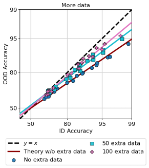
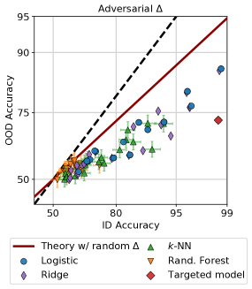
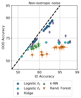
Figure 33: Modifications to our theoretical model showcasing departures from the linear trend. Left: training on auxiliary data related to $D^{\prime}$ (this plot only shows logistic regression models). Middle: choosing the parameter $\boldsymbol{\Delta}$ adversarially to reduce the OOD performance of a particular targeted model. Right: changing the noise covariance to be non-isotropic.

We now detail a number of modifications to our distribution model which break the linear trend predicted by Theorem 1 and shown in Figure 6. In each case, we mathematically define the modified model, provide intuition for why the linear trend no longer holds, and demonstrate the departure from the linear trend via simulation where train prediction models using samples from $D$ and evaluate them on $D^{\prime}$. We defer the full simulation details to the next subsection. The modifications we describe are not the only possible way to depart from the linear fit, but we focus on them because we believe they potentially represent departures from the trend seen in practice,

More data.

Section 5, as well as prior work, show that using additional training data from a broader distribution can cause departure form the linear trend. To simulate such a scenario, we consider a third distribution $D^{\prime\prime}$ defined by $\boldsymbol{x}|y\sim\mathcal{N}(\boldsymbol{\mu}^{\prime\prime}\cdot y;(\sigma^{\prime\prime})^{2}I)$, with $\boldsymbol{\mu}^{\prime\prime}=\boldsymbol{\mu}^{\prime}+\beta\tilde{\boldsymbol{\Delta}}$ and $\tilde{\boldsymbol{\Delta}}$ uniformly distributed on the unit sphere and independent of $\boldsymbol{\Delta}$. (Recall that $\boldsymbol{\mu}^{\prime}=\alpha\boldsymbol{\mu}+\beta\boldsymbol{\Delta}$). Since $D^{\prime\prime}$ is more similar to $D^{\prime}$, we expect that including $D^{\prime\prime}$ samples in the training will result in better OOD performance. However, this inclusion could harm ID performance.

We demonstrate these effects in Figure 33 (left), where we train logistic regression models using samples from $D$ and 0, 50 or 100 samples from $D^{\prime}$, with $\sigma^{\prime\prime}=\sqrt{2}\sigma$ and all other parameters identical to the experiment shown in Figure 6. As expected, the extra data results in better OOD performance but worse ID performance. Moreover, the models trained on each amount of external training data appear to roughly follow linear trends (the plot shows empirical probit linear fits). However, we note that our theoretical analysis does not guarantee such linear fit, because the training data used to compute the classifier depends on $\boldsymbol{\Delta}$ through the samples from $D^{\prime\prime}$.

Adversarial distribution shift.

As previously mentioned, the randomization of the distribution shift was crucial for our assumption, because if we allow $\boldsymbol{\Delta}$ to be a fix deterministic vector we cannot rule out that it depends adversarially on the trained classifier. Let us now spell out the implications of this possibility, by allowing $\boldsymbol{\Delta}$ to be any arbitrary vector of norm at most 1. Given some target classifier given a target classifier $\boldsymbol{\theta}$, suppose pick $\boldsymbol{\Delta}=c\cdot\boldsymbol{\theta}/\|\boldsymbol{\theta}\|=c\cdot\boldsymbol{\theta}/\|\boldsymbol{\theta}\|$ for some $c\in[-1,1]$. This makes the inner product $\hat{\boldsymbol{\theta}}^{\top}\boldsymbol{\Delta}=c$. Recalling Eq. (2), this clearly implies a large departure from the linear trend when $|c|$ is close to 1. In particular, by picking negative $c$ we may substantially reduce the performance of the model on $D^{\prime}$. We note that this form of distribution shift is precisely the Gaussian model of adversarial examples proposed by Schmidt et al. [93].

In Figure 33 (middle), we demonstrate this technique by selecting one of the linear classifiers shown in Figure 6, call it $\boldsymbol{\theta}^{\star}$, and letting $\boldsymbol{\Delta}=-0.03\boldsymbol{\theta}^{\star}/\|\boldsymbol{\theta}^{\star}\|$. As the figure shows, the linear trend breaks substantially, particularly for the targeted classifier.

Non-isotropic covariance shifts.

Finally, we consider the case where the noise covariance under $D$ is not isotropic. That is, we let $\boldsymbol{x}|y\sim\mathcal{N}(\boldsymbol{\mu}\cdot y;\Sigma)$ for some $\Sigma$ that is not a multiple of the identity. Instead of considering shifts to the mean $\boldsymbol{\mu}$, we consider random covariance shifts of the form

$$\Sigma^{\prime}=\Sigma+(\sigma^{\prime})^{2}I_{d\times d},$$

i.e., simple additive white Gaussian noise with variance $\sigma^{\prime}$. Under this distribution shift model, the probit accuracies are

$$\Phi^{-1}\left(\mathrm{acc}_{D}(\boldsymbol{\theta})\right)=\frac{\boldsymbol{\theta}^{\top}\boldsymbol{\mu}}{\sqrt{\boldsymbol{\theta}^{\top}\Sigma\boldsymbol{\theta}}}~{}~{}\mbox{and}~{}~{}\Phi^{-1}\left(\mathrm{acc}_{D^{\prime}}(\boldsymbol{\theta})\right)=\frac{\boldsymbol{\theta}^{\top}\boldsymbol{\mu}}{\sqrt{\boldsymbol{\theta}^{\top}\Sigma^{\prime}\boldsymbol{\theta}}}$$

For a the linear ID-OOD probit accuracy relationship to hold for all $\boldsymbol{\theta}$, we must have that $\Phi^{-1}\left(\mathrm{acc}_{D}(\boldsymbol{\theta})\right)/\Phi^{-1}\left(\mathrm{acc}_{D^{\prime}}(\boldsymbol{\theta})\right)$ is a constant independent of $\boldsymbol{\theta}$, which happens if and only if

$$\frac{\boldsymbol{\theta}^{\top}\Sigma^{\prime}\boldsymbol{\theta}}{\boldsymbol{\theta}^{\top}\Sigma\boldsymbol{\theta}}=1+\frac{\sigma^{\prime 2}\|\boldsymbol{\theta}\|^{2}}{\boldsymbol{\theta}^{\top}\Sigma\boldsymbol{\theta}}$$

is a constant independent of $\boldsymbol{\theta}$. However, this only holds when $\Sigma$ is a multiple of the identity, contradictory to our assumptions. Indeed, whenever $\Sigma$ is not a multiple of the identity, there could be a tradeoff between ID and OOD performance: the former favors $\boldsymbol{\theta}$ with small $\Sigma$-weighted norms, while the latter also depends on the standard Euclidean norm $\|\boldsymbol{\theta}\|^{2}$. Consequently, we expect regularization that limits $\|\boldsymbol{\theta}\|^{2}$ to provide better OOD performance.

Figure 33 (right) demonstrates this phenomenon via simulation. In the figure, we set $\Sigma$ to be diagonal with a portion of the entries close to zero so that giving the corresponding coordinates of $\boldsymbol{\theta}$ larger weight results in better ID accuracy. For the distribution shift we let $(\sigma^{\prime})^{2}=\operatorname{\mathrm{tr}}(\Sigma)/d$. As the figure shows, the linear trend no longer holds, despite the fact that the distribution shift is “only” adding isotropic Gaussian noise to the covariates. Moreover, as the above discussion predicts, the logistic and ridge regression models that attain strong OOD performance are those with stronger $\ell_{2}$ regularization. We also show logistic regression trained classifiers with $\ell_{1}$ regularization—these classifiers do not achieve good OOD performance.

E.3 Simulation details

Below, we provide additional details about the simulations described in Figures 6 and 33.

Training parameters.

We fit logistic regression, ridge regression, nearest neighbors and random forest models using their scikit-learn implementations [76]. For logistic regression we use values of the inverse-regularization parameter $C$ ranging from $10^{-6}$ to $1$; we use $\ell_{2}$ penalty throughout except the covariance shift experiment where we also consider $\ell_{1}$ penalty. For ridge regression we use values of the regularization parameter $\alpha$ ranging from $10^{-3}$ to $10$. For both types of linear models we do not fit an intercept. For nearest neighbors we use $1$ or $3$ nearest neighbors, and for random forests we use $3$, $30$ or $100$ estimators. The remaining parameters are set to their scikit-learn defaults.

In addition to varying the learning hyperparameters described above, to produce models with varying accuracy we also modulate the training set size and dimensionality reduction. To reduce the training set size to size $n_{\mathrm{sub}}$, we pick the first $n_{\mathrm{sub}}$ entries from a fixed training set generated once. To reduce dimensionality down to $d_{\mathrm{proj}}$, we simply pick the first $d_{\mathrm{proj}}$ coordinates of $x$. For the all simulations except covariance shift, we let $n_{\mathrm{sub}}$ range between $30$ and $100$, and use $d_{\mathrm{proj}}$ in the range $50$ to $3000$. In the covariance shift simulation we use $n_{\mathrm{sub}}\in[100,2000]$ and fix $d_{\mathrm{proj}}=d=500$.

Accuracy measurement.

For linear models we compute the accuracy exactly (see Subsection E.1 for closed-form expressions). Consequently, we do not show error bars for these models. For the remaining models we estimate the accuracy on samples from the appropriate distributions and use error bars to show 95% Clopper-Pearson confidence intervals, consistently with the rest of the paper.

Distribution model parameter setting.

Throughout, we pick $\mu$ to be random unit vector (i.e., with the same distribution as $\boldsymbol{\Delta}$). For all simulations except covariance shift, we let $d=10^{5}$, $\sigma=10^{-1.5}$, $\alpha=0.7$, $\beta=0.5$ and $\gamma=1$. For the covariance shift simulation, we found that using a smaller dimension and more training points lead to more noticeable effects. Therefore, for this simulation we let $d=500$ (recall that $\alpha,\beta$ and $\gamma$ do not exist in the covariance shift model). We let the covariance matrix $\Sigma$ be diagonal, with $490$ diagonal entries of size $1/2$ and the remainder of size $1/200$; the locations of the small entries were chosen at random. The shifted covariance is $\Sigma^{\prime}=\Sigma+\frac{1}{8}I_{d\times d}$.

Appendix F Additional related work

We now summarize some of the additional work related to the phenomena we study in our paper. Our focus here is mostly on recent work. For early work on distribution shift, we refer the reader to [78, 107].

PAC-Bayesian analysis of distribution shift.

Performance under distribution shift has also been characterized under the PAC-Bayesian setting where the learning algorithm outputs a posterior distribution over the h hypothesis class [62, 38, 39]. Li and Bilmes [62] directly bound the error on the target distribution (OOD) in terms of the empirical error on a small number of labeled samples from the target and a “divergence prior” which measures some divergence between the source and target domains. Germain et al. [38] relate the OOD performance to the ID performance via a disagreement measure induced by the hypothesis class. These bounds do not explain the linear trends we find in this paper—Li and Bilmes [62] do not relate the source and target error directly, and the bounds in Germain et al. [38] are functionally similar to those of Ben-David et al. [7] where the ID performance is highly predictive of the OOD performance only if they are equal (Figure 1). Germain et al. [39] present a different analysis where the domain divergence appears as a multiplicative term rather than an additive one like in previous bounds. However, this bound expresses a linear relation between the OOD performance and some exponent of the “expected joint error” on the source domain which is different from the ID performance. Furthermore, the bound is an inequality which only provides an upper bound on the OOD performance, while our empirical results require a bound in the other direction as well.

Reliability of machine learning benchmarks.

When assessing the reproducibility and reliability of statistical findings, Yu [115] advocates for considerations of stability of statistical results under perturbations of the model and data. Key to this account is a notion of a stability target that is estimated under changes to the data used to estimate the target. Viewed in this light, our experimental methodology of training models on one distribution and evaluating them on a collection of out-of-distribution test sets corresponds to testing the stability of an appropriately chosen target under perturbations to the test set. The consistent accuracy drops we observe across out-of-distribution test sets suggests that model accuracies are not stable; however, the precise linear trends we find suggest that model rankings are in fact stable. As a consequence, benchmarks like CIFAR-10 or ImageNet where we observe precise linear trends may provide more reliable knowledge about relative model performance than absolute performance on new out-of-distribution test sets.

Theoretical models for linear trends in earlier work on dataset reproduction.

Both Recht et al. [85] and Recht et al. [86] contain simple models for the linear fits observed in their reproductions of CIFAR-10 and ImageNet. Recht et al. [85] propose a mixture model with an “easy” and “hard” component and model the distribution shift as a change in the weigts of these two components. Their model does indeed give a linear fit, but only with linear axis scaling. As we have seen several times throughout this paper, the scatter plots show cleaner linear trends with logit or probit scaling on the axes. It is also not clear what the “easy” and “hard” components correspond to in distribution shifts such as CIFAR-10.1.

Recht et al. [86] developed their model further. Instead of discrete mixture components, each distribution is now parametrized by a Gaussian distribution over the “hardness” of each image. In addition, every model has a scalar “skill” parameter that determines the probability of a model classifying an image with a given hardness correctly. This model now produces linear fits in the probit domain, which yields a closer fit to empirical results. While a continuous hardness parametrization also is more plausible, it is again unclear what this hardness corresponds to.

Neither the models of Recht et al. [85, 86] nor our model of Section 7 allow us to predict where linear trends occur in actual data; such predictive power is important because—as we demonstrate—some distributions do not yield linear trends. However, our theoretical analysis is based on a concrete generative is based on a concrete generative, rather than postulated abstract properties of data and classifiers. One advantage of this fact is that it allows us to consider modifications of our generative models which show departures from the linear trend, as we do in Appendix E.2.

Linear trends in image classification with natural language supervision.

Among other results, Radford et al. [80] show two important phenomena that are closely related to this paper. First, their training approach (contrastive language image pre-training, “CLIP”), which combines a large training set and natural language supervision, produces image classifiers substantially above the linear trend given by a wide range of ImageNet model in the distribution shift testbed of Taori et al. [104]. This result provides further evidence for the hypothesis that training data plays an important role in the linear trends we describe in this paper. Second, Radford et al. [80] find that once their training set is fixed and they vary model architecture (ResNet variants and Vision Transformers [37]) and compute available for training, the resulting models again follow a clear linear trend. This demonstrates that linear trends between in-distribution and out-of-distribution accuracy occur in a diverse range of settings.

Linear trends under sub-population shift.

One specific type of distribution shift is sub-population shift. In sub-population shift, each class is composed of a set of sub-populations, e.g., the “dog” class in an image classification task may be composed of images from a specific set of dog breeds. A natural goal then is that a trained classifier should generalize to previously unseen dog breeds and still correctly labels them as “dog”. Hendrycks and Dietterich [46] found that a set of eight convolutional neural networks follow a linear trend on a sub-population shift derived from ImageNet-22K. Santurkar et al. [92] construct a range of sub-population shifts from ImageNet and find approximately linear trends for several of the shifts they consider. Their testbed contained 13 convolutional neural networks, some of them with interventions such as adversarial training [68]. Some of the plots in [92] are not directly comparable to ours since they display a relative accuracy measure on the y-axes, not the absolute accuracy (i.e., average 0-1 loss).

Underspecification as defined in D’Amour et al. [30].

D’Amour et al. [30] conduct a broad empirical study and show that out-of-distribution performance can vary widely even for models with the same in-distribution performance. Since this result may at first glance disagree with our results here, we now discuss their empirical results most relevant to our paper in detail. In particular, we focus on their results in computer vision domains.

• D’Amour et al. [30] point out ImageNet-C as an example of underspecification in image classification. Similar to [104], we also find in Figure 24 that some of the perturbations in ImageNet-C show substantial variation as a function of ImageNet accuracy. In addition, we find that this variation occurs in CIFAR-10-C. As mentioned before, not all shifts in ImageNet-C and CIFAR-10-C are affected by underspecification, with some shifts exhibiting comparatively clean linear trends.

• The second example for underspecification in image classification is ObjectNet [5]. While it is indeed true that the accuracy variation on ObjectNet may increase compared to ImageNet, overall ObjectNet still shows predictable behavior as a function of ImageNet accuracy. See Figure 2 in [104].

• In addition to standard computer vision benchmarks, D’Amour et al. [30] also investigate two medical imaging datasets, which give an important complementary perspective. In the first dataset (ophthalmological imaging), they find evidence of underspecification. In the second dataset (dermatological imaging), the evidence is less clear since the tests for statistically significant variation in the four domains give p-values of 0.54, 0.42, 0.29, and 0.03. While the fourth p-value is below 0.05, the authors did not correct for multiple hypothesis testing and remark that this is an exploratory data analysis.

Overall, we find that the empirical evidence for underspecification in computer vision tasks is nuanced. As in our work, some distribution shifts studied by D’Amour et al. [30] exhibit stronger correlation between in-distribution and out-of-distribution than others. Hence there is no clear contradiction between our results and those of D’Amour et al. [30]. Understanding when precise linear trends occur and when underspecification is dominant is an important direction for future work.

Further distribution shifts without universal linear trends.

While we have seen several distribution shifts with clean linear trends between in-distribution and out-of-distribution generalization in this paper, there are also obvious counterexamples. One prominent counterexample are adversarial distribution shifts, e.g., $\ell_{p}$ adversarial examples [10, 99, 9]. For models trained without a robustness intervention, it is usually easy to construct adversarial examples that cause the model to misclassify most inputs despite high accuracy on unperturbed examples. While adversarial robustness is far from solved, it is now possible to train CIFAR-10 networks with about 65% accuracy against the common $\ell_{\infty}$ adversary with $\varepsilon=8/255$ and standard (unperturbed) accuracy of 91% [40]. Since CIFAR-10 classifiers without a robustness intervention have only 0–10% robust accuracy in this setting, it is clear that there cannot be a precise linear trend between in-distribution and out-of-distribution accuracy. Adversarial distribution shifts can bring about departures from the linear trend in our theoretical setup as well, as we discuss in Appendix E.2. We refer the reader to Taori et al. [104] and Hendrycks et al. [47] for additional examples of models not following a linear trend in ImageNet variants, e.g., on some of the ImageNet-C corruptions and ImageNet-R.

Benchmarks for distribution shift.

Recently several groups conducted broad empirical surveys of distribution shift, comparing a wide range of available methods. Most closely related to our paper is Taori et al. [104], where the authors also find clean linear trends on multiple distribution shifts related to ImageNet. Djolonga et al. [35] also observed high correlations on the same distribution shifts for a smaller number of models. Both experiments were limited to ImageNet as in-distribution test set and convolutional neural networks. Here we study multiple different in-distribution datasets for image classification, an additional task (pose estimation), and several models beyond convolutional neural networks.

Gulrajani and Lopez-Paz [41] conduct a broad survey of algorithms for the closely related problem of domain generalization. In domain generalization, the training set is drawn from multiple distinct domains, and the learning algorithm has access to the domain labels. At test time, the trained models is evaluated on samples from a new domain. Gulrajani and Lopez-Paz [41] found that on a range of datasets, current domain generalization algorithms perform only as well or worse as an empirical risk minimization baseline that ignores the domain structure. At a high level, this result is similar to the aforementioned distribution shift benchmarks that also found small or no gains from current robustness interventions on most distribution shifts.

Our results raise similar questions as these benchmarks for distribution shift and domain generalization: when and how is it possible to improve over empirical risk minimization as a baseline for robustness to distribution shift, i.e., to “go above the line” in our scatter plots?

Training methods to improve robustness.

Researchers have proposed a large number of robustness interventions over the past few years. Due to the volume of papers, we only refer to recent surveys here. Methods for improving robustness divide into two categories: those which use samples from the target distribution (which we refer to as the OOD data), and those that do not. The former methods are usually called transfer learning and domain adaptation methods [74, 110]. These methods typically assume that the target distribution data is more constrained than the in-distribution data, either lacking labels or having smaller quantity, and algorithms focus on mitigating these issues. The linear trends observed by Kornblith et al. [56] in the context of transfer learning suggest that there may be important similarities. See Robey et al. [88] for one example applying such techniques to the WILDS OOD shifts considered in this work.

While domain adaptation and transfer learning techniques are helpful in many settings, they are not always applicable. For instance, when we want an autonomous vehicle to drive safely in a new town it has not visited before, we have no additional training data available to adapt the car’s perception system. Such scenarios motivate our study of the correlation between in-distribution and out-of-distribution generalization in this paper. The second category of training methods—sometimes referred to as domain robustness or domain generalization—attempt to learn models that are reliable in the presence of distribution shifts for which there is no direct training data. Instead, these methods often leverage data from multiple other, related domains. Gulrajani and Lopez-Paz [41] provide an overview of current methods for domain generalization.

References

- Andreassen et al. [2021] Anders Andreassen, Yasaman Bahri, Behnam Neyshabur, and Rebecca Roelofs. The evolution of out-of-distribution robustness throughout fine-tuning, 2021. https://arxiv.org/abs/2106.15831.
- Augustin and Hein [2020] Maximilian Augustin and Matthias Hein. Out-distribution aware self-training in an open world setting, 2020. https://arxiv.org/abs/2012.12372.
- Ball [1997] Keith Ball. An elementary introduction to modern convex geometry. Flavors of geometry, 1997. http://library.msri.org/books/Book31/files/ball.pdf.
- Bandi et al. [2018] Peter Bandi, Oscar Geessink, Quirine Manson, Marcory van Dijk, Maschenka Balkenhol, Meyke Hermsen, Babak Ehteshami Bejnordi, Byungjae Lee, Kyunghyun Paeng, Aoxiao Zhong, Quanzheng Li, Farhad Ghazvinian Zanjani, Svitlana Zinger, Keisuke Fukuta, Daisuke Komura, Vlado Ovtcharov, Shenghua Cheng, Shaoqun Zeng, Jeppe Thagaard, Anders B. Dahl, Huangjing Lin, Hao Chen, Ludwig Jacobsson, Martin Hedlund, Melih Çetin, Eren Halıcı, Hunter Jackson, Richard Chen, Fabian Both, Jörg Franke, Heidi Küsters-Vandevelde, Willem Vreuls, Peter Bult, Bram van Ginneken, Jeroen van der Laak, and Geert Litjens. From detection of individual metastases to classification of lymph node status at the patient level: the CAMELYON17 challenge. IEEE Transactions on Medical Imaging, 2018. https://ieeexplore.ieee.org/document/8447230.
- Barbu et al. [2019] Andrei Barbu, David Mayo, Julian Alverio, William Luo, Christopher Wang, Dan Gutfreund, Josh Tenenbaum, and Boris Katz. ObjectNet: A large-scale bias-controlled dataset for pushing the limits of object recognition models. Advances in Neural Information Processing Systems (NeurIPS), 2019. https://objectnet.dev/.
- Beery et al. [2020] Sara Beery, Elijah Cole, and Arvi Gjoka. The iWildCam 2020 competition dataset. In Fine-Grained Visual Categorization Workshop at the Conference on Computer Vision and Pattern Recognition (CVPR), 2020. https://arxiv.org/abs/2004.10340.
- Ben-David et al. [2006] Shai Ben-David, John Blitzer, Koby Crammer, and Fernando Pereira. Analysis of representations for domain adaptation. In Advances in neural information processing systems (NeurIPS), 2006. https://papers.nips.cc/paper/2006/hash/b1b0432ceafb0ce714426e9114852ac7-Abstract.html.
- Ben-David et al. [2010] Shai Ben-David, John Blitzer, Koby Crammer, Alex Kulesza, Fernando Pereira, and Jennifer Wortman Vaughan. A theory of learning from different domains. Machine learning, 2010. https://link.springer.com/article/10.1007/s10994-009-5152-4.
- Biggio and Roli [2018] Battista Biggio and Fabio Roli. Wild patterns: Ten years after the rise of adversarial machine learning. Pattern Recognition, 2018. https://arxiv.org/abs/1712.03141.
- Biggio et al. [2013] Battista Biggio, Igino Corona, Davide Maiorca, Blaine Nelson, Nedim Šrndić, Pavel Laskov, Giorgio Giacinto, and Fabio Roli. Evasion attacks against machine learning at test time. In European Conference on Machine Learning and Principles and Practice of Knowledge Discovery in Databases (ECMLPKDD), 2013. https://arxiv.org/abs/1708.06131.
- Blender Online Community [2021] Blender Online Community. Blender - a 3D modelling and rendering package. Blender Foundation, Blender Institute, Amsterdam, 2021. http://www.blender.org.
- Blitzer et al. [2007] John Blitzer, Koby Crammer, Alex Kulesza, Fernando Pereira, and Jennifer Wortman. Learning bounds for domain adaptation. In Advances in Neural Information Processing Systems (NeurIPS), 2007. https://papers.nips.cc/paper/2007/hash/42e77b63637ab381e8be5f8318cc28a2-Abstract.html.
- Bradski [2000] G. Bradski. The OpenCV Library. Dr. Dobb’s Journal of Software Tools, 2000. https://opencv.org/.
- Breiman [2001] Leo Breiman. Random forests. Machine learning, 2001. https://link.springer.com/article/10.1023/A:1010933404324.
- Brown et al. [2020] Tom Brown, Benjamin Mann, Nick Ryder, Melanie Subbiah, Jared D Kaplan, Prafulla Dhariwal, Arvind Neelakantan, Pranav Shyam, Girish Sastry, Amanda Askell, Sandhini Agarwal, Ariel Herbert-Voss, Gretchen Krueger, Tom Henighan, Rewon Child, Aditya Ramesh, Daniel Ziegler, Jeffrey Wu, Clemens Winter, Chris Hesse, Mark Chen, Eric Sigler, Mateusz Litwin, Scott Gray, Benjamin Chess, Jack Clark, Christopher Berner, Sam McCandlish, Alec Radford, Ilya Sutskever, and Dario Amodei. Language models are few-shot learners. In Advances in Neural Information Processing Systems (NeurIPS), 2020. https://arxiv.org/abs/2005.14165.
- Caine et al. [2021] Benjamin Caine, Rebecca Roelofs, Vijay Vasudevan, Jiquan Ngiam, Yuning Chai, Zhifeng Chen, and Jonathon Shlens. Pseudo-labeling for scalable 3D object detection, 2021. https://arxiv.org/abs/2103.02093.
- Calli et al. [2015] Berk Calli, Aaron Walsman, Arjun Singh, Siddhartha Srinivasa, Pieter Abbeel, and Aaron M Dollar. Benchmarking in manipulation research: The YCB object and model set and benchmarking protocols, 2015. https://arxiv.org/abs/1502.03143.
- Carmon et al. [2019] Yair Carmon, Aditi Raghunathan, Ludwig Schmidt, and John Duchi. Unlabeled data improves adversarial robustness. In Advances in Neural Information Processing Systems (NeurIPS), 2019. https://arxiv.org/abs/1905.13736.
- Caron et al. [2020] Mathilde Caron, Ishan Misra, Julien Mairal, Priya Goyal, Piotr Bojanowski, and Armand Joulin. Unsupervised learning of visual features by contrasting cluster assignments. In Advances in Neural Information Processing Systems (NeurIPS), 2020. https://arxiv.org/abs/2006.09882.
- Chaurasia and Culurciello [2017] Abhishek Chaurasia and Eugenio Culurciello. LinkNet: exploiting encoder representations for efficient semantic segmentation. In Visual Communications and Image Processing (VCIP), 2017. https://arxiv.org/abs/1707.03718.
- Chen et al. [2020] Ting Chen, Simon Kornblith, Kevin Swersky, Mohammad Norouzi, and Geoffrey Hinton. Big self-supervised models are strong semi-supervised learners. In Advances in Neural Information Processing Systems (NeurIPS), 2020. https://arxiv.org/abs/2006.10029.
- Chen and He [2020] Xinlei Chen and Kaiming He. Exploring simple siamese representation learning, 2020. https://arxiv.org/abs/2011.10566.
- Chen et al. [2017] Yunpeng Chen, Jianan Li, Huaxin Xiao, Xiaojie Jin, Shuicheng Yan, and Jiashi Feng. Dual path networks. In Advances in Neural Information Processing Systems (NeurIPS), 2017. https://arxiv.org/abs/1707.01629.
- Chollet [2017] François Chollet. Xception: Deep learning with depthwise separable convolutions. In Conference on Computer Vision and Pattern Recognition (CVPR), 2017. https://arxiv.org/abs/1610.02357.
- Christie et al. [2018] Gordon Christie, Neil Fendley, James Wilson, and Ryan Mukherjee. Functional map of the world. In Conference on Computer Vision and Pattern Recognition (CVPR), 2018. https://arxiv.org/abs/1711.07846.
- Coates and Ng [2012] Adam Coates and Andrew Y Ng. Learning feature representations with k-means. In Neural networks: Tricks of the trade. Springer, 2012. https://www-cs.stanford.edu/~acoates/papers/coatesng_nntot2012.pdf.
- Coates et al. [2011] Adam Coates, Andrew Ng, and Honglak Lee. An analysis of single-layer networks in unsupervised feature learning. In International Conference on Artificial Intelligence and Statistics (AISTATS), 2011. http://proceedings.mlr.press/v15/coates11a.html.
- Cohen et al. [2019] Jeremy Cohen, Elan Rosenfeld, and Zico Kolter. Certified adversarial robustness via randomized smoothing. In International Conference on Machine Learning (ICML), 2019. https://arxiv.org/abs/1902.02918.
- Cubuk et al. [2020] Ekin D Cubuk, Barret Zoph, Jonathon Shlens, and Quoc V Le. RandAugment: practical automated data augmentation with a reduced search space. In Advances in Neural Information Processing Systems (NeurIPS), 2020. https://papers.nips.cc/paper/2020/hash/d85b63ef0ccb114d0a3bb7b7d808028f-Abstract.html.
- D’Amour et al. [2020] Alexander D’Amour, Katherine Heller, Dan Moldovan, Ben Adlam, Babak Alipanahi, Alex Beutel, Christina Chen, Jonathan Deaton, Jacob Eisenstein, Matthew D. Hoffman, Farhad Hormozdiari, Neil Houlsby, Shaobo Hou, Ghassen Jerfel, Alan Karthikesalingam, Mario Lucic, Yian Ma, Cory McLean, Diana Mincu, Akinori Mitani, Andrea Montanari, Zachary Nado, Vivek Natarajan, Christopher Nielson, Thomas F. Osborne, Rajiv Raman, Kim Ramasamy, Rory Sayres, Jessica Schrouff, Martin Seneviratne, Shannon Sequeira, Harini Suresh, Victor Veitch, Max Vladymyrov, Xuezhi Wang, Kellie Webster, Steve Yadlowsky, Taedong Yun, Xiaohua Zhai, and D. Sculley. Underspecification presents challenges for credibility in modern machine learning, 2020. https://arxiv.org/abs/2011.03395.
- Darestani et al. [2021] Mohammad Zalbagi Darestani, Akshay Chaudhari, and Reinhard Heckel. Measuring robustness in deep learning based compressive sensing. In International Conference on Machine Learning (ICML), 2021. https://arxiv.org/abs/2102.06103.
- Darlow et al. [2018] Luke N Darlow, Elliot J Crowley, Antreas Antoniou, and Amos J Storkey. CINIC-10 is not ImageNet or CIFAR-10, 2018. https://arxiv.org/abs/1810.03505.
- Deng et al. [2009] Jia Deng, Wei Dong, Richard Socher, Li-Jia Li, Kai Li, and Li Fei-Fei. ImageNet: A large-scale hierarchical image database. In Conference on Computer Vision and Pattern Recognition (CVPR), 2009. http://www.image-net.org/papers/imagenet_cvpr09.pdf.
- Devlin et al. [2018] Jacob Devlin, Ming-Wei Chang, Kenton Lee, and Kristina Toutanova. BERT: pre-training of deep bidirectional transformers for language understanding. 2018. http://arxiv.org/abs/1810.04805.
- Djolonga et al. [2021] Josip Djolonga, Jessica Yung, Michael Tschannen, Rob Romijnders, Lucas Beyer, Alexander Kolesnikov, Joan Puigcerver, Matthias Minderer, Alexander D’Amour, Dan Moldovan, Sylvan Gelly, Neil Houlsby, Xiaohua Zhai, and Mario Lucic. On robustness and transferability of convolutional neural networks. In Conference on Computer Vision and Pattern Recognition (CVPR), 2021. https://arxiv.org/abs/2007.08558.
- Donahue et al. [2014] Jeff Donahue, Yangqing Jia, Oriol Vinyals, Judy Hoffman, Ning Zhang, Eric Tzeng, and Trevor Darrell. Decaf: A deep convolutional activation feature for generic visual recognition. In International Conference on Machine Learning (ICML), 2014. https://arxiv.org/abs/1310.1531.
- Dosovitskiy et al. [2021] Alexey Dosovitskiy, Lucas Beyer, Alexander Kolesnikov, Dirk Weissenborn, Xiaohua Zhai, Thomas Unterthiner, Mostafa Dehghani, Matthias Minderer, Georg Heigold, Sylvain Gelly, Jakob Uszkoreit, and Neil Houlsby. An image is worth 16x16 words: Transformers for image recognition at scale. In International Conference on Learning Representations (ICLR), 2021. https://arxiv.org/abs/2010.11929.
- Germain et al. [2013] Pascal Germain, Amaury Habrard, François Laviolette, and Emilie Morvant. A pac-bayesian approach for domain adaptation with specialization to linear classifiers. In International conference on machine learning (ICML), 2013. http://proceedings.mlr.press/v28/germain13.html.
- Germain et al. [2016] Pascal Germain, Amaury Habrard, François Laviolette, and Emilie Morvant. A new PAC-Bayesian perspective on domain adaptation. In International conference on machine learning (ICML), 2016. https://arxiv.org/abs/1506.04573.
- Gowal et al. [2020] Sven Gowal, Chongli Qin, Jonathan Uesato, Timothy Mann, and Pushmeet Kohli. Uncovering the limits of adversarial training against norm-bounded adversarial examples. https://arxiv.org/abs/2010.03593, 2020.