REX: Revisiting Budgeted Training with an Improved Schedule

Abstract.

Deep learning practitioners often operate on a computational and monetary budget. Thus, it is critical to design optimization algorithms that perform well under any budget. The linear learning rate schedule is considered the best budget-aware schedule (Li et al., 2020), as it outperforms most other schedules in the low budget regime. On the other hand, learning rate schedules –such as the 30-60-90 step schedule– are known to achieve high performance when the model can be trained for many epochs. Yet, it is often not known a priori whether one’s budget will be large or small; thus, the optimal choice of learning rate schedule is made on a case-by-case basis. In this paper, we frame the learning rate schedule selection problem as a combination of $i)$ selecting a profile (i.e., the continuous function that models the learning rate schedule), and $ii)$ choosing a sampling rate (i.e., how frequently the learning rate is updated/sampled from this profile). We propose a novel profile and sampling rate combination called the Reflected Exponential (REX) schedule, which we evaluate across seven different experimental settings with both SGD and Adam optimizers. REX outperforms the linear schedule in the low budget regime, while matching or exceeding the performance of several state-of-the-art learning rate schedules (linear, step, exponential, cosine, step decay on plateau, and OneCycle) in both high and low budget regimes. Furthermore, REX requires no added computation, storage, or hyperparameters.

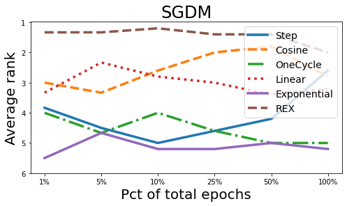
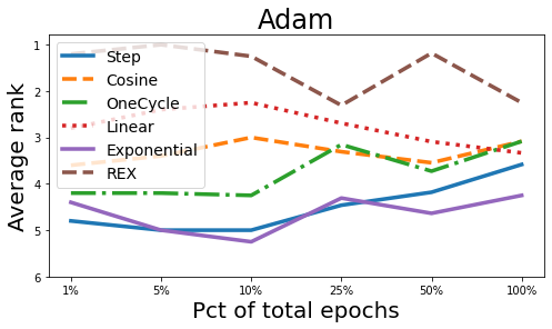
Figure 1. We summarize all 82 experimental settings, including image classification, object detection, and natural language processing. We plot the average ranked performance of the considered learning rate schedules, where 1 is the best and 6 is the worst, against the training budget, for the momentum SGD (SGDM) and Adam optimizers. The maximum epochs (100%) is determined from the literature and verified to achieve previously reported results. Each % of total epochs is an independent run. The schedules are adjusted for each setting to maintain the same profile (e.g. the linear schedule decays the learning rate linearly to 0 regardless of the % of total epochs). For smaller epochs, the linear schedule performs well while the performance of the step schedule in higher epochs does not carry over. The proposed REX schedule outperforms all methods in comparison, in both high and low epochs.

Table 1. Performance of different schedules, ranked according to the % of Top-1 or Top-3 finishes, out of a total of 28 experiments. Top-1 (Top-3) refers to the best (best-3) performance for a particular model/dataset/base optimizer/epoch setting. Low (high) budget includes 1%, 5%, and 10% (25%, 50%, and 100%) of the full epochs. The Decay on Plateau variant is aggregated into the Step Schedule method where we take the max performance for each setting.

	Low budget ($<$25%)		High budget ($\geq$25%)		Overall
Method	Top-1	Top-3	Top-1	Top-3	Top-1	Top-3
None	0%	0%	2%	10%	1%	5%
Exp decay (Abadi et al., 2015; Paszke et al., 2017)	5%	7%	5%	14%	5%	11%
OneCycle (Smith, 2018)	15%	49%	12%	40%	13%	45%
Linear Schedule (Abadi et al., 2015; Paszke et al., 2017)	10%	78%	12%	62%	11%	70%
Step Schedule (He et al., 2016)	2%	12%	7%	38%	5%	25%
Cosine Schedule (Loshchilov and Hutter, 2017b)	2%	66%	10%	62%	6%	64%
REX	73%	95%	67%	88%	70%	92%

1. Introduction

While hardware has consistently improved (Sze et al., 2017; Shawahna et al., 2019), the cost of training deep neural networks (DNNs) has continued to increase due to growth in the size of models and datasets (Krizhevsky et al., 2012; Devlin et al., 2019; Brown et al., 2020; Chen et al., 2020a). One key component of the cost is the need to tune the hyperparameters of the model (Yang and Shami, 2020). Outside of the largest companies in the field, most practitioners have to trade-off the number of epochs with the number of experimental trials. Whilst the community has generally agreed that, for example, 90 epochs is a reasonable training length for a ResNet-50 architecture on ImageNet (He et al., 2016; Huang et al., 2017; Zagoruyko and Komodakis, 2016), there simply may not be sufficient monetary budget to perform such extensive training for certain projects. Further, it is generally not easy to predict the number of epochs required to maximize the performance of the model apriori, particularly if the input data may be continually changing. Thus, it is important to consider the optimization of DNNs for a diverse range of budgets.

Stochastic Gradient Descent (SGD) with momentum and Adam are two of the most widely used optimizers for DNNs (He et al., 2016; Huang et al., 2017; Zagoruyko and Komodakis, 2016; Devlin et al., 2019; Brown et al., 2020; Redmon and Farhadi, 2018). Whether the task is image classification, object detection, or fine-tuning in natural language processing, both optimizers must be combined with some form of learning rate decay to achieve good performance (He et al., 2016; Huang et al., 2017; Zagoruyko and Komodakis, 2016; Devlin et al., 2019; Brown et al., 2020; Redmon and Farhadi, 2018) (see Tables 4-11). The aforementioned tasks are arguably the most widely used applications of deep learning.

The learning rate schedule is particularly important in the budgeted training setting. Moreover, of the widely used schedules, the best learning rate schedule for a small number of epochs is generally not the best for a large number of epochs (see Tables 4-11). This is a significant challenge, since it is difficult to know apriori if the current budget lies in the high or low budget regime. This raises two questions: Can we close the budget-induced gap in the performance of existing learning rate schedules? And, if this is not possible, is there a learning rate schedule that performs well in both low and high budget regimes?

We answer both questions through a novel lens. We decompose the problem of selecting a learning rate schedule as a two-part process of $i)$ selecting a profile and $ii)$ selecting a sampling rate. The profile is the function that models the learning rate schedule, and the sampling rate is how frequently the learning rate is updated, based on this profile. In this view, we $i)$ analyze existing schedules, $ii)$ propose a novel profile and sampling rate combination, and $iii)$ benchmark the performance of numerous schedules. We also demonstrate it is possible to boost the performance of existing learning rate schedules by introducing a hyperparameter that delays the commencement of the decay schedule. However, because adding an extra hyperparameter is prohibitive in the budgeted setting, we also propose a new schedule, REX, which performs at a state-of-the-art level for both low and high budgets across a large variety of settings without the extra hyperparameter tuning.

Specifically, our contributions are as follows:

• We pose learning rate schedules as the combination of a profile and a sampling rate and identify that there is no optimal profile for all sampling rates. Namely, we show that no existing, popular learning rate schedule achieves state-of-the-art performance in both high and low budget regimes.

• We propose a new profile and sampling rate combination. We find that carefully tuning the start of the learning rate decay for existing schedules can result in significant performance improvements in both high and low budget regimes. However, this introduces an extra hyperparameter, which is prohibitive for budget-limited practitioners. Our proposed schedule can be understood as an interpolation between the linear schedule and the delayed variants.

• Our proposed schedule, REX, is based on observations of the above, and we validate its state-of-the-art performance across seven settings, including image classification, object detection, and natural language processing.

Our goal is to introduce an easy-to-use, state-of-the-art learning rate schedule with no extra hyperparameters that performs well in all budget regimes and can be easily implemented and adopted.

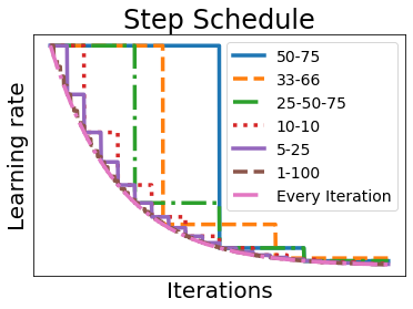
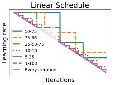
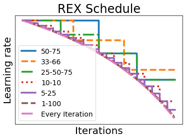
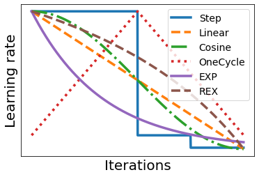
Figure 2. Popular schedules with various sampling rates. 50-75 refers to sampling once at 50% and 75% of total epochs. Similarly for 33-66 and 25-50-75. 10-10 refers to sampling once every 10% of total epochs. Similarly for 5-25 and 1-100. Every iteration is the maximum sampling rate. Left: Step schedule. Left Middle: Linear Schedule. Right Middle: REX Schedule. Right: Schedules with their usual sampling rate.

2. Related Works

There have been many works related to tuning the learning rate. There is a connection between learning rate and momentum (Yuan et al., 2016), and there are methods which alter the momentum (Sutskever et al., 2013; Zhang and Mitliagkas, 2017; O’donoghue and Candes, 2015; Lucas et al., 2018; Chen et al., 2020b). There is also a connection between learning rate and batch sizes (Smith et al., 2017; You et al., 2017; Goyal et al., 2018). The most popular learning rate tuning mechanisms fall into two categories: Automatically tuning the learning rate on a per-weight basis and decaying the learning rate globally.

Many adaptive learning rate optimizers have been proposed. Modern learning rate adaptive methods began with AdaGrad (Duchi et al., 2011), which was shown to have good convergence properties, especially in the sparse gradient setting. AdaDelta (Zeiler, 2012) was proposed to fix a units issue with AdaGrad. RMSprop (Hinton et al., 2012) employed a running estimate of the second moment to resolve the strictly decreasing learning rate of AdaGrad. The most popular adaptive learning rate optimizer is Adam (Kingma and Ba, 2014) and its variants (Loshchilov and Hutter, 2017a; Liu et al., 2020). Yet, in practice, adaptive learning rate algorithms perform the best when coupled with a learning rate schedule (Devlin et al., 2019; Liu et al., 2020).

In deep learning, the step schedule was widely used in early computer vision work (Krizhevsky et al., 2012; He et al., 2016; Huang et al., 2017). This was often combined with SGD with Momentum to achieve state-of-the-art results (He et al., 2016; Zagoruyko and Komodakis, 2016; Huang et al., 2017; Redmon et al., 2016). In Natural Language Processing, AdamW (Loshchilov and Hutter, 2017a) is often paired with a cosine or linear learning rate decay for training and fine-tuning transformers (Wolf et al., 2020). The aforementioned schedules are widely available and implemented in the most popular software (Wolf et al., 2020; Abadi et al., 2015; Paszke et al., 2017), in addition to the exponential decay schedule, OneCycle (Smith, 2018), cosine decay with restarts (Loshchilov and Hutter, 2017b) and others (Smith, 2017). While some schedules may be preferred for achieving state-of-the-art results, it has been suggested that the linear schedule is most suitable for the low budget scenario (Li et al., 2020), which may be of more relevance to practitioners.

3. Budgeted Training: Profiles and Sampling Rates

Challenges in adapting learning rate schedules to the budgeted setting. The primary hyperparameter in DNN optimization is the initial learning rate. While good heuristics often exist for tuning common hyperparameters, such as setting momentum $\beta=0.9$ or setting a 30-60-90 learning rate schedule (Zagoruyko and Komodakis, 2016; Huang et al., 2017; Hu et al., 2017), the initial learning rate remains to be tuned. However, in the budgeted training setting, the learning rate schedule turns into a hyperparameter. Adapting, for example, the 30-60-90 rule for Image Classification or Object Detection is not straightforward, and naively following the same rules for a smaller number of epochs results in sub-optimal results (see Step Schedule in low epoch settings in Tables 4-11). Additionally, following the 50-75 rule (He et al., 2016) on RN20-CIFAR10 for a training budget that is 1% of the usual total epochs can result a 5% absolute error gap with the best-performing schedule. We assume that, in the budgeted training setting, the number of epochs is still pre-defined, but can be significantly less than the usual total epochs.

Profiles and sampling rates. To formalize the process of identifying a good learning rate schedule, we decompose the learning rate schedule as a combination of a profile curve and a sampling rate on that curve. The profile is the function that models the learning rate schedule and dictates the general curve of the learning rate schedule. In most –but not all (Li and Arora, 2020)– applications, this function starts at a high initial value and ends near zero. The sampling rate is how frequently the learning rate is updated and dictates the smoothness of the curve. At one extreme, the linear learning rate schedule, and many others, samples from the profile at each iteration, and at the other extreme the step learning rate schedules samples only twice or thrice across the entire training procedure. For example, the 50-75 step schedule can be approximated as sampling twice from a particular, exponentially-decaying profile. See Figure 2 for some examples of schedules with their associated profile and sampling rates.

Lack of an optimal profile. While there may be limited motivation to pick a particular sampling rate, this introduces an interesting question: Does there exist an optimal profile for all reasonable sampling rates? In Table 2, we benchmark three profiles: $i)$ the 50-75 step schedule (He et al., 2016) approximated as a tuned exponentially decaying profile ; $ii)$ the linear profile (Abadi et al., 2015; Paszke et al., 2017); and, $iii)$ the REX profile proposed in this paper (to be defined in the next subsection). These three profiles represent smoothly-decaying learning rate schedules with varying curvatures. We find that different profiles perform best for different sampling rates. The approximated Step schedule profile performs best with low sampling rates, while the linear and REX profiles perform best with high sampling rates. Furthermore, the approximated Step schedule profile performs worst for a small and medium number of epochs and best for a high number of epochs. The REX profile performs best for a small and medium number of epochs. While the Step schedule is consistently used to achieve state-of-the-art results in Computer Vision (He et al., 2016; Zagoruyko and Komodakis, 2016; Huang et al., 2017; Hu et al., 2017; Redmon et al., 2016; He et al., 2018), it does not translate directly to lower epoch settings.

Table 2. We demonstrate learning rate schedules and sampling rates on RN20-CIFAR10-SGDM (Top) and RN38-CIFAR10-SGDM (Bottom) (He et al., 2016), holding the learning rate constant. There is no best profile for all sampling rates. Each profile excels at one end of the spectrum. 50-75 (He et al., 2016) refers to sampling once at 50% and 75% of total epochs. Similarly for 33-66 and 25-50-75. 10-10 refers to sampling once every 10% of total epochs. Similarly for 5-25 and 1-100. Every iteration is the maximum sampling rate.

RN20-CIFAR10-SGDM	15 Epochs			75 Epochs			300 Epochs
Sampling Rate	Step	Linear	REX	Step	Linear	REX	Step	Linear	REX
50-75	14.48	16.96	20.79	9.44	12.42	18.05	7.32	10.15	12.41
33-66	17.89	25.80	24.45	9.72	13.38	15.98	7.93	11.90	11.43
25-50-75	16.52	18.77	26.13	9.73	12.31	12.59	8.46	8.26	12.31
10-10	17.98	16.35	16.48	10.41	9.40	11.17	8.67	8.26	8.24
5-25	18.87	13.83	15.17	9.79	8.94	9.22	8.85	8.24	8.50
1-100	18.53	13.91	13.34	10.61	8.72	8.60	9.20	7.97	7.74
Every Iteration	19.19	13.09	12.86	9.97	8.89	8.37	9.24	7.62	7.52
RN38-CIFAR10-SGDM	15 Epochs			75 Epochs			300 Epochs
Sampling Rate	Step	Linear	REX	Step	Linear	REX	Step	Linear	REX
50-75	13.57	17.31	18.47	7.59	12.89	14.38	6.66	10.07	9.37
33-66	14.96	19.16	18.71	7.74	13.64	17.57	6.70	11.53	11.30
25-50-75	15.69	14.18	19.77	7.99	9.10	15.07	6.73	7.59	8.44
10-10	16.58	13.34	14.46	7.87	8.33	9.75	7.60	6.48	6.50
5-25	17.16	12.63	11.71	8.40	7.42	7.13	8.79	6.18	6.41
1-100	17.20	11.93	11.13	8.54	7.06	7.17	9.11	6.12	6.17
Every Iteration	17.97	12.11	10.95	8.72	7.10	6.86	9.31	5.89	6.09

A new profile. Since there is no profile which performs optimally across sampling rates, it remains to ask if there is a profile and sampling rate combination that results in strong performance in both low and high epoch settings. Therefore, we propose the Reflected Exponential (REX) profile; see Figure 2. REX is an alternative to the linear and exponential profile, and we find that REX has stronger empirical performance in the budgeted setting. REX performs best with a per-iteration sampling rate, similar to the linear schedule. We evaluate the performance of REX extensively in following sections.

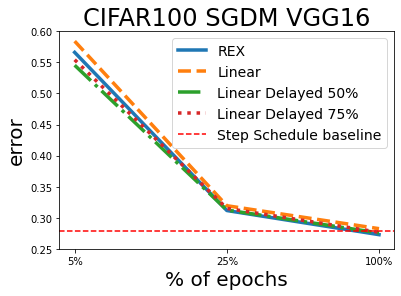
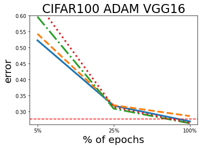
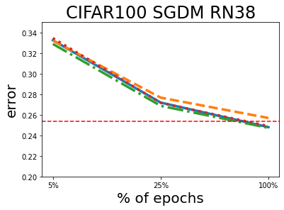
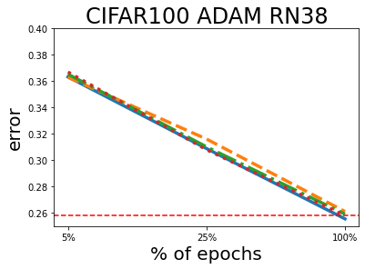
Figure 3. REX, linear, and delayed linear schedules. Left: VGG16-CIFAR100-SGDM. Left Middle: VGG16-CIFAR100-ADAM. Right Middle: RN38-CIFAR100-SGDM. Right: RN38-CIFAR100-ADAM. The red dashed line represents the error of the step schedule for that setting trained with 100% of the epochs. Linear Delayed X% refers to delaying the linear decay till X% of the total epochs have passed, before decaying linearly to 0. For example, in the left-middle plot, for small % of epochs, REX outperforms the linear schedule, which outperforms the delayed variants. However, for large epochs, the linear schedule is unable to achieve the state-of-the-art performance of the step schedule, while REX and the delayed linear schedules are able to surpass the step schedule.

We also motivate REX with the empirical observation that the linear schedule can be improved in some cases by delaying the onset of the decay, i.e., holding the initial learning rate constant until XX% of the budget, and then linearly decaying the learning rate to 0; see Figure 3. In particular, it appears that performance can be improved with such delay in the high epoch regime, but this strategy is less effective with fewer epochs. However, the exact onset of the delay introduces an additional hyperparameter. REX can be understood as an interpolation between a linear schedule and a delayed linear schedule without additional hyperparameters. Furthermore, REX generally outperforms the linear schedule, which has been previously suggested as the best budgeted schedule (Li et al., 2020), for small and large epochs.

It appears that certain schedules have reasonable performance across sampling rates, while others have poor or state-of-the-art performance depending on the sampling rate. If the sampling rate is unknown or there is a particular reason to select a low sampling rate, the approximated step profile appears to be the best choice. However, in most applications, the sampling rate is a choice by the practitioner. Since the REX profile with a per-iteration sampling rate generally performs the best, there may be limited motivation to use alternative schedules.

Table 3. Summary of experimental settings.

Experiment short name	Model	Dataset	Maximum Epochs
RN20-CIFAR10	ResNet20	CIFAR10	300 (He et al., 2016)
RN50-IMAGENET	ResNet50	ImageNet	90 (Huang et al., 2017)
VGG16-CIFAR100	VGG-16	CIFAR100	300 (He et al., 2016)
WRN-STL10	Wide ResNet 16-8	STL10	200 (Chang et al., 2017)
VAE-MNIST	VAE	MNIST	200 (Yeung et al., 2017)
YOLO-VOC	YOLOv3	Pascal VOC	50 (Tripathi et al., 2016)
BERTBASE-GLUE	BERT (Pre-trained)	GLUE (9 tasks)	3 (Devlin et al., 2019)

Table 4. RN20-CIFAR10. The number of epochs was predefined before the execution of the algorithms. Bold red indicates Top-1 performance, black bold is Top-3.

SGDM	1%	5%	10%	25%	50%	100%
+ Step Schedule	32.14 $\pm$ .34	14.94 $\pm$ .27	11.80 $\pm$ .11	8.82 $\pm$ .25	8.43 $\pm$ .07	7.32 $\pm$ .14
+ Cosine Schedule	28.49 $\pm$ .25	13.05 $\pm$ .17	10.62 $\pm$ .29	8.80 $\pm$ .08	8.10 $\pm$ .13	7.78 $\pm$ .14
+ OneCycle	40.14 $\pm$ 2.62	18.93 $\pm$ 1.85	12.74 $\pm$ .36	10.83 $\pm$ .25	9.23 $\pm$ .19	8.42 $\pm$ .12
+ Linear Schedule	28.70 $\pm$ 1.13	13.09 $\pm$ .13	10.85 $\pm$ .15	9.03 $\pm$ .24	8.15 $\pm$ .12	7.62 $\pm$ .12
+ Decay on Plateau	41.98 $\pm$ 3.20	25.93 $\pm$ .45	11.29 $\pm$ .35	9.05 $\pm$ .07	8.26 $\pm$ .07	7.97 $\pm$ .14
+ Exp decay	31.31 $\pm$ 1.34	14.85 $\pm$ .38	11.56 $\pm$ .22	9.55 $\pm$ .09	9.20 $\pm$ .13	7.82 $\pm$ .05
+ REX	27.94 $\pm$ .46	12.86 $\pm$ .27	10.23 $\pm$ .13	8.37 $\pm$ .09	7.52 $\pm$ .24	7.52 $\pm$ .05
Adam	42.10 $\pm$ 2.71	23.01 $\pm$ 1.10	16.58 $\pm$ .18	13.63 $\pm$ .22	11.90 $\pm$ .06	11.94 $\pm$ .06
+ Step Schedule	30.72 $\pm$ .16	15.41 $\pm$ .26	12.20 $\pm$ .11	10.47 $\pm$ .10	8.75 $\pm$ .17	8.55 $\pm$ .05
+ Cosine Schedule	29.20 $\pm$ .24	14.31 $\pm$ .28	11.45 $\pm$ .27	9.56 $\pm$ .12	9.15 $\pm$ .12	8.93 $\pm$ .07
+ OneCycle	37.17 $\pm$ 2.49	16.16 $\pm$ .19	14.11 $\pm$ .57	10.33 $\pm$ .20	9.87 $\pm$ .12	9.03 $\pm$ .18
+ Linear Schedule	28.99 $\pm$ .37	14.08 $\pm$ .34	10.97 $\pm$ .19	9.25 $\pm$ .12	9.20 $\pm$ .22	8.89 $\pm$ .05
+ Decay on Plateau	43.40 $\pm$ 4.57	22.21 $\pm$ .96	13.46 $\pm$ .38	9.71 $\pm$ .39	8.92 $\pm$ .18	8.80 $\pm$ .11
+ Exp decay	31.87 $\pm$ .59	15.82 $\pm$ .06	12.91 $\pm$ .21	10.48 $\pm$ .15	9.24 $\pm$ .16	8.53 $\pm$ .07
+ REX	27.64 $\pm$ .02	13.96 $\pm$ .16	10.88 $\pm$ .05	9.44 $\pm$ .22	8.72 $\pm$ .24	8.18 $\pm$ .15

4. Results

In this section we present results in all seven experimental settings given in Table 3, including image classification, image generation, object detection and natural language processing. For fair evaluation in the budgeted training scenario, only the learning rate is tuned in multiples of 3 for each schedule, setting, and number of epochs. All reported metrics are averaged across three separate trials. We run all settings at 1%, 5%, 10%, 25%, 50%, and 100% of maximum epochs, representing both low and high budgets. In each setting, the learning rate schedule is concerned only with the total epochs for that run, e.g., the linear schedule will decay linearly to 0 regardless if the budget is 1% or 100% of the maximum epochs. For BERT_BASE-GLUE, results are given for 1 run and at $\nicefrac{{1}}{{3}}$, $\nicefrac{{2}}{{3}}$, and $\nicefrac{{3}}{{3}}$ of total epochs. The maximum total epochs is determined from commonly used epochs in the literature, and validated to achieve the reported score in the literature. The maximum epochs is given in Table 3. The goal is to demonstrate performance in both the low and high budget regime across a range of common applications to instill confidence that the proposed schedule will work “in the wild”. We use a model-dataset-optimizer notation, e.g. RN20-CIFAR10-SGDM means a ResNet20 model trained on CIFAR10 with momentum SGD.

Table 5. WRN-STL10. The number of epochs was predefined before the execution of the algorithms. Bold red indicates Top-1 performance, black bold is Top-3.

SGDM	1%	5%	10%	25%	50%	100%
+ Step Schedule	60.09 $\pm$ 1.15	38.12 $\pm$ .32	33.86 $\pm$ .10	22.42 $\pm$ .56	17.20 $\pm$ .35	14.51 $\pm$ .26
+ Cosine Schedule	57.81 $\pm$ 1.05	37.42 $\pm$ .29	27.51 $\pm$ .25	20.03 $\pm$ .26	17.02 $\pm$ .24	14.66 $\pm$ .25
+ OneCycle	58.75 $\pm$ .76	36.90 $\pm$ .37	26.97 $\pm$ .27	21.67 $\pm$ .27	19.69 $\pm$ .21	19.00 $\pm$ .42
+ Linear Schedule	58.74 $\pm$ 1.26	34.81 $\pm$ .40	28.17 $\pm$ .64	19.54 $\pm$ .20	17.39 $\pm$ .24	14.58 $\pm$ .18
+ Decay on Plateau	59.64 $\pm$ .92	37.64 $\pm$ 1.44	36.94 $\pm$ 1.96	21.05 $\pm$ .27	17.83 $\pm$ .39	15.16 $\pm$ .36
+ Exp decay	60.21 $\pm$ .77	38.94 $\pm$ 1.08	34.11 $\pm$ .77	22.65 $\pm$ .49	20.60 $\pm$ .21	15.85 $\pm$ .28
+ REX	55.93 $\pm$ .46	34.50 $\pm$ .16	25.52 $\pm$ .17	20.54 $\pm$ .32	16.97 $\pm$ .46	14.60 $\pm$ .31
Adam	58.65 $\pm$ 1.79	42.66 $\pm$ .68	33.17 $\pm$ 1.94	23.35 $\pm$ .20	19.63 $\pm$ .26	18.65 $\pm$ .07
+ Step Schedule	59.35 $\pm$ .98	47.14 $\pm$ .42	35.10 $\pm$ 1.10	23.85 $\pm$ .07	19.63 $\pm$ .33	18.29 $\pm$ .10
+ Cosine Schedule	58.95 $\pm$ .95	40.69 $\pm$ 1.09	31.00 $\pm$ .74	22.85 $\pm$ .47	21.47 $\pm$ .31	19.08 $\pm$ .36
+ OneCycle	57.88 $\pm$ .88	36.41 $\pm$ .29	27.90 $\pm$ .63	20.02 $\pm$ .19	19.21 $\pm$ .28	19.03 $\pm$ .43
+ Linear Schedule	56.72 $\pm$ .22	40.25 $\pm$ 1.00	31.15 $\pm$ .29	21.70 $\pm$ .11	21.53 $\pm$ .44	17.85 $\pm$ .15
+ Decay on Plateau	58.72 $\pm$ .60	42.30 $\pm$ .68	33.00 $\pm$ .80	22.77 $\pm$ .33	19.91 $\pm$ .45	19.61 $\pm$ .56
+ Exp decay	58.92 $\pm$ .52	44.76 $\pm$ .90	33.52 $\pm$ 1.18	23.30 $\pm$ .39	20.70 $\pm$ .50	19.63 $\pm$ .24
+ REX	56.47 $\pm$ .31	35.52 $\pm$ .44	27.24 $\pm$ .20	21.65 $\pm$ .21	19.12 $\pm$ .31	17.75 $\pm$ .22

Table 6. VGG16-CIFAR100 generalization error. The number of epochs was predefined before the execution of the algorithms. Bold red indicates Top-1 performance, black bold is Top-3.

SGDM	1%	5%	10%	25%	50%	100%
+ Step Schedule	95.03 $\pm$ .42	69.87 $\pm$ .28	46.97 $\pm$ .13	35.04 $\pm$ .24	30.09 $\pm$ .32	27.83 $\pm$ .30
+ Cosine Schedule	95.03 $\pm$ .42	61.82 $\pm$ .13	41.26 $\pm$ .26	31.93 $\pm$ .09	28.63 $\pm$ .11	27.84 $\pm$ .12
+ OneCycle	91.96 $\pm$ 1.01	58.35 $\pm$ .40	45.39 $\pm$ .73	32.62 $\pm$ .21	30.10 $\pm$ .34	29.09 $\pm$ .12
+ Linear Schedule	96.11 $\pm$ 1.64	58.14 $\pm$ 1.19	39.66 $\pm$ .61	31.95 $\pm$ .29	29.10 $\pm$ .34	28.26 $\pm$ .08
+ Decay on Plateau	94.70 $\pm$ 1.20	65.25 $\pm$ 1.72	50.81 $\pm$ .58	35.29 $\pm$ .59	30.65 $\pm$ .31	29.74 $\pm$ .43
+ Exp decay	96.54 $\pm$ .39	65.65 $\pm$ 1.24	49.04 $\pm$ 1.98	33.15 $\pm$ .19	29.51 $\pm$ .22	28.47 $\pm$ .18
+ REX	94.92 $\pm$ .91	56.62 $\pm$ .65	40.72 $\pm$ .29	31.16 $\pm$ .11	28.54 $\pm$ .02	27.27 $\pm$ .30
Adam	92.70 $\pm$ .50	64.05 $\pm$ .41	57.56 $\pm$ 1.30	37.98 $\pm$ .20	33.62 $\pm$ .11	31.09 $\pm$ .09
+ Step Schedule	92.65 $\pm$ .38	62.90 $\pm$ .08	44.94 $\pm$ .49	34.16 $\pm$ .11	29.40 $\pm$ .22	27.75 $\pm$ .15
+ Cosine Schedule	91.48 $\pm$ .42	55.90 $\pm$ 2.46	40.31 $\pm$ .07	32.32 $\pm$ .14	29.68 $\pm$ .17	28.08 $\pm$ .10
+ OneCycle	92.18 $\pm$ .69	58.29 $\pm$ .53	43.47 $\pm$ .28	34.59 $\pm$ .31	29.83 $\pm$ .29	29.58 $\pm$ .18
+ Linear Schedule	92.94 $\pm$ .49	54.32 $\pm$ 1.17	39.49 $\pm$ .11	32.01 $\pm$ .49	29.30 $\pm$ .18	28.65 $\pm$ .10
+ Decay on Plateau	92.76 $\pm$ .48	64.10 $\pm$ .22	57.05 $\pm$ .84	32.60 $\pm$ .31	29.03 $\pm$ .10	28.67 $\pm$ .19
+ Exp decay	92.43 $\pm$ .67	55.26 $\pm$ 1.24	42.62 $\pm$ .12	32.37 $\pm$ .18	29.53 $\pm$ .12	28.83 $\pm$ .08
+ REX	91.93 $\pm$ .01	52.20 $\pm$ .47	39.51 $\pm$ .21	31.68 $\pm$ .57	28.58 $\pm$ .16	26.99 $\pm$ .09

4.1. Learning Rate Schedules

There are many popular learning rate schedules implemented in widely-used frameworks and packages. In general, the schedules are aware of the current time step $t$ and the maximum time step $T$. Let $\eta$ denote the learning rate and $\beta$ the momentum. We comprehensively detail the schedules considered in this paper below, covering almost all widely-implemented schedules; see Figure 2 for a visualization.

• Step schedule (He et al., 2016): $\eta_{t}=\gamma_{t}\cdot\eta_{0}$ where $\gamma_{t}$ is piece-wise and depends on $\nicefrac{{t}}{{T}}$. A typical schedule (He et al., 2016) would be to decay the learning rate by $0.1$ at $\nicefrac{{1}}{{2}}$ epochs and again by $0.1$ at $\nicefrac{{3}}{{4}}$ epochs. We employ such a step schedule for all our experiments.

• Decay on Plateau (Abadi et al., 2015; Paszke et al., 2017): A practical version of the step schedule, where the learning rate is decayed when the validation loss does not improve for certain number of tuneable epochs, which we tune in multiples of 5.

• Linear schedule (Abadi et al., 2015; Paszke et al., 2017): $\eta_{t}=\left(1-\nicefrac{{t}}{{T}}\right)\cdot\eta_{0}$.

• Cosine schedule (Loshchilov and Hutter, 2017b): $\eta_{t}=\tfrac{\eta_{0}}{2}\cdot\left(1+\cos(\tfrac{\pi\cdot t}{T})\right)$.

• Exponential schedule (Abadi et al., 2015; Paszke et al., 2017): $\eta_{t}=\eta_{0}\cdot e^{\nicefrac{{\gamma t}}{{T}}}$. We find that setting $\gamma=-3$ yields the best performance.

• OneCycle schedule (Smith, 2018):

  $$\eta_{t}=\begin{cases}\eta_{\min}+(\eta_{\max}-\eta_{\min})\cdot\left(\tfrac{t}{\nicefrac{{T}}{{2}}}\right)\cdot\eta_{0},&\textbf{if}~{}~{}\nicefrac{{t}}{{T}}<1/2\\ \eta_{\min}+(\eta_{\max}-\eta_{\min})\cdot\left(2-\tfrac{t}{\nicefrac{{T}}{{2}}}\right)\cdot\eta_{0},&\text{otherwise}\end{cases}$$

  $$\beta_{t}=\begin{cases}\beta_{\min}+(\beta_{\max}-\beta_{\min})\cdot\left(1-\tfrac{t}{\nicefrac{{T}}{{2}}}\right)\cdot\beta_{0},&\textbf{if}~{}~{}\nicefrac{{t}}{{T}}<1/2\\ \beta_{\min}+(\beta_{\max}-\beta_{\min})\cdot\left(\tfrac{t}{\nicefrac{{T}}{{2}}}-1\right)\cdot\beta_{0},&\text{otherwise}\end{cases}$$

  $\eta_{\min}$, $\eta_{\max}$, $\beta_{\min}$, and $\beta_{\max}$ are hyperparameters. For fair computational comparison, we follow the recommended settings (Smith, 2018) and set $\eta_{\min}=\eta_{\max}\cdot 0.1$, $\beta_{\max}=0.95$, $\beta_{\min}=0.85$, so that $\eta_{\max}$ is the only hyperparameter.

• REX schedule:

  $$\eta_{t}=\eta_{0}\cdot\left(\frac{1-\nicefrac{{t}}{{T}}}{\nicefrac{{1}}{{2}}+\nicefrac{{1}}{{2}}\cdot(1-\nicefrac{{t}}{{T}})}\right).$$

  We re-emphasize the motivation for REX: it is a new profile and sampling rate combination, which is motivated by the improved performance of a delayed linear schedule in certain circumstances. REX aggressively decreases the learning rate towards the end of the training process, which is the “reflection” of the exponential decay.

There are simply too many schedules to compare comprehensively, so we select the widely-used schedules above for comparison. We apply the schedules to the two most popular optimizers: SGD with momentum and Adam.

4.2. Empirical Results

Table 7. VAE-MNIST generalization loss. The number of epochs was predefined before the execution of the algorithms. Bold red indicates Top-1 performance, black bold is Top-3, ignoring non SGDM and Adam optimizers.

SGDM	1%	5%	10%	25%	50%	100%
+ Step Schedule	180.30 $\pm$ 6.98	152.97 $\pm$ .55	146.24 $\pm$ 2.50	140.28 $\pm$ .51	137.70 $\pm$ .93	136.34 $\pm$ .31
+ Cosine Schedule	174.52 $\pm$ 1.09	145.99 $\pm$ .15	141.23 $\pm$ .36	139.15 $\pm$ .26	136.69 $\pm$ .27	135.05 $\pm$ .09
+ OneCycle	161.95 $\pm$ .67	146.25 $\pm$ .35	143.01 $\pm$ 1.08	139.79 $\pm$ .66	137.20 $\pm$ .06	135.65 $\pm$ .44
+ Linear Schedule	174.64 $\pm$ .15	146.15 $\pm$ .26	143.64 $\pm$ .80	148.00 $\pm$ .48	141.72 $\pm$ .48	137.84 $\pm$ .32
+ Decay on Plateau	167.16 $\pm$ .30	151.15 $\pm$ .11	146.82 $\pm$ .58	140.51 $\pm$ .73	139.54 $\pm$ .34	137.33 $\pm$ .49
+ Exp decay	179.60 $\pm$ 3.47	160.52 $\pm$ .64	146.24 $\pm$ .73	154.31 $\pm$ .43	145.83 $\pm$ .48	139.67 $\pm$ .57
+ REX	149.85 $\pm$ 1.62	139.56 $\pm$ .78	137.15 $\pm$ .05	134.41 $\pm$ .78	135.69 $\pm$ .24	135.03 $\pm$ .37
Adam	152.10 $\pm$ .55	142.54 $\pm$ .50	140.10 $\pm$ .82	136.28 $\pm$ .18	134.64 $\pm$ .14	134.66 $\pm$ .17
+ Step Schedule	153.45 $\pm$ 1.47	142.19 $\pm$ .98	138.32 $\pm$ .20	136.62 $\pm$ .30	134.14 $\pm$ .56	133.34 $\pm$ .41
+ Cosine Schedule	149.82 $\pm$ .32	140.78 $\pm$ .72	137.66 $\pm$ .79	134.73 $\pm$ .04	133.25 $\pm$ .26	133.23 $\pm$ .30
+ OneCycle	149.07 $\pm$ .99	139.75 $\pm$ .27	138.12 $\pm$ .99	134.67 $\pm$ .55	133.27 $\pm$ .07	132.83 $\pm$ .33
+ Linear Schedule	148.93 $\pm$ .20	139.82 $\pm$ .20	137.00 $\pm$ .70	134.71 $\pm$ .25	134.00 $\pm$ .49	132.95 $\pm$ .24
+ Decay on Plateau	152.08 $\pm$ .45	141.54 $\pm$ .31	139.76 $\pm$ .52	135.68 $\pm$ .59	134.10 $\pm$ .21	134.06 $\pm$ .45
+ Exp decay	149.28 $\pm$ .46	142.94 $\pm$ 1.28	138.82 $\pm$ .36	135.19 $\pm$ .43	134.05 $\pm$ .16	133.88 $\pm$ .85
+ REX	148.59 $\pm$ .33	139.05 $\pm$ .20	136.62 $\pm$ .21	134.24 $\pm$ .02	133.16 $\pm$ .05	132.52 $\pm$ .05

Image Classification. We choose four diverse settings for this task. For datasets, we use the standard CIFAR10 and CIFAR100 datasets, in addition to the low count, high-res STL10 dataset, as well as the standard ImageNet dataset. Since ResNets remain the most commonly-deployed model in industry, we perform experiments with three variations of the ResNet (He et al., 2016). The ResNet20 comes from the line of lower cost, lower performance ResNets, and is a close cousin of the more expensive and better performing ResNet18. ResNet50 belongs to the latter series, and is a standard model for ImageNet. We also include the Wide ResNet variation which further increases the model width for better performance (Zagoruyko and Komodakis, 2016). The other model we employ is the VGG-16 model (Simonyan and Zisserman, 2014). While VGG models are far outdated in attaining state-of-the-art performance, the architecture is still relevant for custom applications with smaller CNNs, where residual connections have limited application. We provide thorough evaluation in the RN20-CIFAR10, WRN-STL10, VGG16-CIFAR100 settings, and, due to computational constraints, provide lower epochs results for RN50-ImageNet, given in Tables 4, 5, 6, and 8.

As observed in (Li et al., 2020), the linear schedule performs well for both SGD and Adam, particularly for a low number of epochs. While the Step schedule performs well for the maximum number of epochs, it scales very poorly to lower epoch settings. On the other hand, REX performs well in both high and low epoch regimes. Results also follow general Computer Vision observations for these settings, where SGD tends to outperform Adam.

Table 8. RN50-ImageNet generalization error. The number of epochs was predefined before the execution of the algorithms. Bold red indicates Top-1 performance, black bold is Top-3.

SGDM	1%	5%
+ Step Schedule	87.28	46.58
+ Cosine Schedule	82.88	43.90
+ OneCycle	90.94	55.00
+ Linear Schedule	82.00	43.27
+ Exp decay	90.19	48.28
+ REX	80.98	40.78
Adam	1%	5%
+ Step Schedule	77.97	45.91
+ Cosine Schedule	73.51	43.66
+ OneCycle	82.58	62.57
+ Linear Schedule	71.42	42.01
+ Exp decay	75.54	45.43
+ REX	69.91	40.65

Table 9. YOLO-VOC mAP. The number of epochs was predefined before the execution of the algorithms. Bold red indicates Top-1 performance, black bold is Top-3.

	1%	5%	10%	25%	50%	100%
Adam	45.0 $\pm$ 3.4	48.1 $\pm$ 7.6	61.9 $\pm$ 1.8	70.2 $\pm$ 3.5	72.1 $\pm$ 6.4	79.1 $\pm$ 1.6
+ Step Schedule	62.2 $\pm$ 1.7	67.0 $\pm$ 3.4	71.8 $\pm$ 1.0	78.5 $\pm$ 0.2	81.1 $\pm$ 1.0	83.2 $\pm$ 0.2
+ OneCycle	60.4 $\pm$ 7.2	63.8 $\pm$ 7.6	74.9 $\pm$ 1.0	79.9 $\pm$ 1.3	81.1 $\pm$ 2.8	83.3 $\pm$ 0.4
+ Cosine Schedule	63.6 $\pm$ 5.2	66.8 $\pm$ 6.1	75.9 $\pm$ 0.2	81.1 $\pm$ 0.7	82.5 $\pm$ 1.0	84.0 $\pm$ 0.2
+ Linear Schedule	63.7 $\pm$ 5.5	67.2 $\pm$ 5.9	76.2 $\pm$ 0.7	81.1 $\pm$ 0.9	82.4 $\pm$ 1.2	83.4 $\pm$ 0.2
+ Exp decay	49.6 $\pm$ 24	68.1 $\pm$ 4.6	75.6 $\pm$ 0.1	80.1 $\pm$ 0.7	81.2 $\pm$ 2.2	83.2 $\pm$ 0.2
+ REX	64.0 $\pm$ 5.0	67.0 $\pm$ 6.5	76.7 $\pm$ 0.3	81.2 $\pm$ 0.7	82.2 $\pm$ 1.8	83.4 $\pm$ 0.4

Image Generation. The two most popular types of networks for image generation are Variational Encoders (VAE) (Kingma and Welling, 2015) and Generative Adversarial Networks (GAN) (Goodfellow et al., 2014). However, out of the two, only VAEs consistently benefit from learning rate decay (Goodfellow et al., 2014; Chen et al., 2016; Arjovsky et al., 2017; Brock et al., 2019; Hou et al., 2016; Sonderby et al., 2016; Vahdat and Kautz, 2021). Therefore, we select VAEs as the network of choice for image generation. We train VAEs on the MNIST dataset for 200 epochs, after which performance no longer improves. Results are given in Table 7.

The linear schedule performs well for Adam, but not for SGDM. Similarly, the cosine schedule performs well for SGDM, but not for Adam. The OneCycle schedule performs well across all settings, but REX outperforms all other schedules in the low budget and high budget setting.

Object Detection. We train a YOLOv3 (Redmon and Farhadi, 2018) model on the Pascal VOC dataset. The training set is the combined 2007 and 2012 training set, and the test set is the 2007 test set. We were able to achieve the mAP score reported in the literature by training the network for 50 epochs. Thus, we set this as the maximum number of epochs. We find that the network does not train well without a warm-up period, so all networks are trained for 2 epochs from a learning rate of 1e-5 linearly increased to 1e-4. This warm-up phase is not counted as part of the allocated training budget. We also round up the number of epochs to the closest integer: for example, the 1% setting trains for 2 warmup epochs and then $\lceil 50\cdot 0.01\rceil=1$ epoch, for a total of 3 epochs. The 100% setting trains for 2 warmup epochs and then 50 epochs for a total of 52 epochs. Results are given in Table 9. Similar to other settings, the step schedule performs reasonably well for a large number of epochs, but is outperformed by the cosine schedule. REX performs well in the low epoch setting.

Natural Language Processing. Fine-tuning pre-trained transformer models is one of the most common training procedures in NLP (Devlin et al., 2019; Brown et al., 2020), thus making it a setting of interest. This is because $i)$ it is often cost-prohibitive for practitioners to pre-train their own models and $ii)$ fine-tuning pre-trained transformers often results in significantly better performance in comparison to training a smaller model from scratch. The linear schedule is the default schedule implemented in HuggingFace (Wolf et al., 2020), the most popular package for transformer models, and is considered the gold standard in this domain. We fine-tune BERT_BASE on the GLUE benchmark, an NLP benchmark with nine datasets. We leave out the problematic WNLI dataset (Devlin et al., 2019). Since we are able to attain the scores reported in the literature with 3 epochs of fine-tuning, we set that as the maximum number of epochs. Due to computational constraints, we can only perform one run per setting, which causes some variability within the results. Although REX achieves the best mean score for small and large budgets, we see that the best optimizer can vary depending on the dataset. For example, OneCycle attains the best scores on QNLI and MRPC, and the Cosine schedule performs the best on SST-2.

Table 10. Results of BERT_BASE-GLUE. AdamW + Linear Schedule follows the huggingface (Wolf et al., 2020) implementation, and achieves the results in well-known studies (Devlin et al., 2019; Sanh et al., 2020). Results given by 1 epoch/2 epochs/3 epochs. Excluding the problematic WNLI dataset (Devlin et al., 2019).

	Score
AdamW	79.9/81.2/81.8
+ Step Schedule	80.2/81.9/82.3
+ Cosine Schedule	80.9/82.2/82.7
+ OneCycle	81.0/82.0/82.7
+ Linear Schedule	81.2/82.3/82.6
+ Exp decay	80.6/81.8/82.5
+ REX	81.7/82.6/82.8

Table 11. Results of BERT_BASE-GLUE. AdamW + Linear Schedule follows the huggingface (Wolf et al., 2020) implementation, and achieves the results in well-known studies (Devlin et al., 2019; Sanh et al., 2020). Results given by 1 epoch/2 epochs/3 epochs. Excluding the problematic WNLI dataset (Devlin et al., 2019).

	CoLA	MNLI	MRPC	QNLI	QQP	RTE	SST-2	STS-B
AdamW	54.8/54.7/55.2	82.9/83.3/83.7	84.8/87.2/87.6	88.7/90.4/90.7	89.4/90.2/90.5	59.2/64.6/66.8	91.2/91.3/91.2	87.8/87.8/88.3
+ Step Schedule	53.5/56.9/56.6	82.6/83.4/83.9	85.6/87.9/88.3	88.2/90.1/90.4	89.0/90.5/90.6	63.5/65.7/67.5	92.8/92.8/93.0	86.7/88.0/88.4
+ Cosine Schedule	55.7/58.6/58.2	83.5/84.0/84.2	84.5/87.6/87.9	89.4/89.8/90.4	89.8/90.6/91.0	64.2/65.3/67.5	92.7/93.1/93.7	87.4/88.4/88.7
+ OneCycle	57.7/58.1/56.5	83.6/83.8/84.2	87.3/87.5/89.9	89.5/91.0/90.7	89.8/90.6/90.8	60.3/63.9/67.5	92.1/92.2/93.0	88.1/88.5/89.0
+ Linear Schedule	58.0/57.6/58.8	83.5/84.1/84.3	85.4/88.1/88.0	88.8/90.4/89.6	89.7/90.6/91.0	63.5/65.7/67.1	92.8/93.0/92.9	87.9/88.5/88.8
+ Exp decay	57.5/57.3/59.1	83.6/83.9/84.1	86.2/88.7/89.1	88.2/89.2/89.6	88.8/90.3/90.6	61.0/63.9/66.0	92.1/93.1/93.0	87.2/88.2/88.5
+ REX	57.8/58.8/59.1	83.4/84.0/84.3	87.3/88.9/89.1	88.9/90.5/90.3	90.0/90.7/91.0	65.3/66.8/67.1	92.7/92.7/92.7	87.6/88.6/88.6

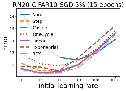
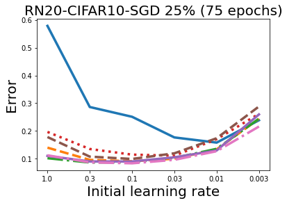
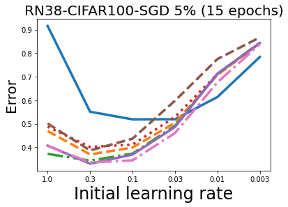
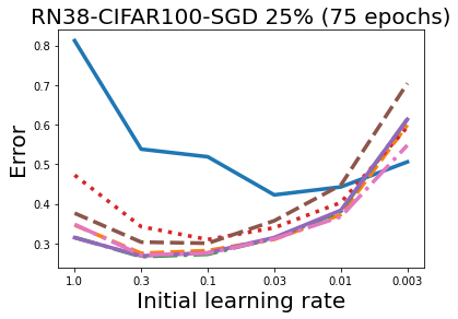
Figure 4. Error against initial learning for RN20-CIFAR10-SGD and RN38-CIFAR100-SGD for 5% and 25% of total epochs. As expected all, schedules suffer as the learning rate grows too large or too small.

Sensitivity to learning rate tuning. While it is reasonable to suggest that the practitioner simply pick a per-iteration sampling rate for the REX, linear, and other profiles, a relevant issue in budgeted training is performance given a limited number of experimental trials. Namely, in extreme cases, the practitioner may not even have the budget to finely tune the learning rate. Therefore, we plot the considered schedules in two settings against learning rate, presented in Figure 4. Clearly, there is no schedule that can recover from a poor initial learning rate. However, schedules tend to retain their relative ordering across initial learning rates. This means that even with poor hyperparameter settings, the choice of learning rate schedule remains important. REX, represented by the pink line below all other lines, outperforms other schedules for most learning rates in the budgeted settings presented in the plots.

5. Conclusion

In this paper, we identified issues with existing learning rate schedules in the budgeted setting. We proposed a profile and sampling rate framework for understanding existing schedules. While there is no optimal profile, we found that the proposed REX schedule performs well with a sampling rate of every iteration in both small and large epoch regimes. With thorough empirical evaluation, we confirm that the proposed REX learning rate schedule performs favorably across a large number of settings including image classification, generation, object detection, and natural language processing.

References

- (1)
- Abadi et al. (2015) Martín Abadi, Ashish Agarwal, Paul Barham, Eugene Brevdo, Zhifeng Chen, Craig Citro, Greg S. Corrado, Andy Davis, Jeffrey Dean, Matthieu Devin, Sanjay Ghemawat, Ian Goodfellow, Andrew Harp, Geoffrey Irving, Michael Isard, Yangqing Jia, Rafal Jozefowicz, Lukasz Kaiser, Manjunath Kudlur, Josh Levenberg, Dan Mané, Rajat Monga, Sherry Moore, Derek Murray, Chris Olah, Mike Schuster, Jonathon Shlens, Benoit Steiner, Ilya Sutskever, Kunal Talwar, Paul Tucker, Vincent Vanhoucke, Vijay Vasudevan, Fernanda Viégas, Oriol Vinyals, Pete Warden, Martin Wattenberg, Martin Wicke, Yuan Yu, and Xiaoqiang Zheng. 2015. TensorFlow: Large-Scale Machine Learning on Heterogeneous Systems. http://tensorflow.org/ Software available from tensorflow.org.
- Arjovsky et al. (2017) Martin Arjovsky, Soumith Chintala, and Léon Bottou. 2017. Wasserstein GAN. arXiv:1701.07875 [stat.ML]
- Brock et al. (2019) Andrew Brock, Jeff Donahue, and Karen Simonyan. 2019. Large Scale GAN Training for High Fidelity Natural Image Synthesis. arXiv:1809.11096 [cs.LG]
- Brown et al. (2020) Tom B. Brown, Benjamin Mann, Nick Ryder, Melanie Subbiah, Jared Kaplan, Prafulla Dhariwal, Arvind Neelakantan, Pranav Shyam, Girish Sastry, Amanda Askell, Sandhini Agarwal, Ariel Herbert-Voss, Gretchen Krueger, Tom Henighan, Rewon Child, Aditya Ramesh, Daniel M. Ziegler, Jeffrey Wu, Clemens Winter, Christopher Hesse, Mark Chen, Eric Sigler, Mateusz Litwin, Scott Gray, Benjamin Chess, Jack Clark, Christopher Berner, Sam McCandlish, Alec Radford, Ilya Sutskever, and Dario Amodei. 2020. Language Models are Few-Shot Learners. arXiv:2005.14165 [cs.CL]
- Chang et al. (2017) Bo Chang, Lili Meng, Eldad Haber, Lars Ruthotto, David Begert, and Elliot Holtham. 2017. Reversible Architectures for Arbitrarily Deep Residual Neural Networks. arXiv:1709.03698 [cs.CV]
- Chen et al. (2020b) John Chen, Cameron Wolfe, Zhao Li, and Anastasios Kyrillidis. 2020b. Demon: Momentum Decay for Improved Neural Network Training. arXiv:1910.04952 [cs.LG]
- Chen et al. (2020a) Ting Chen, Simon Kornblith, Kevin Swersky, Mohammad Norouzi, and Geoffrey Hinton. 2020a. Big Self-Supervised Models are Strong Semi-Supervised Learners. arXiv:2006.10029 [cs.LG]
- Chen et al. (2016) Xi Chen, Yan Duan, Rein Houthooft, John Schulman, Ilya Sutskever, and Pieter Abbeel. 2016. InfoGAN: Interpretable Representation Learning by Information Maximizing Generative Adversarial Nets. arXiv:1606.03657 [cs.LG]
- Devlin et al. (2019) Jacob Devlin, Ming-Wei Chang, Kenton Lee, and Kristina Toutanova. 2019. BERT: Pre-training of Deep Bidirectional Transformers for Language Understanding. arXiv:1810.04805 [cs.CL]
- Duchi et al. (2011) John Duchi, Elad Hazan, and Yoram Singer. 2011. Adaptive subgradient methods for online learning and stochastic optimization. Journal of Machine Learning Research 12, Jul (2011), 2121–2159.
- Goodfellow et al. (2014) Ian J. Goodfellow, Jean Pouget-Abadie, Mehdi Mirza, Bing Xu, David Warde-Farley, Sherjil Ozair, Aaron Courville, and Yoshua Bengio. 2014. Generative Adversarial Networks. arXiv:1406.2661 [stat.ML]
- Goyal et al. (2018) Priya Goyal, Piotr Dollár, Ross Girshick, Pieter Noordhuis, Lukasz Wesolowski, Aapo Kyrola, Andrew Tulloch, Yangqing Jia, and Kaiming He. 2018. Accurate, Large Minibatch SGD: Training ImageNet in 1 Hour. arXiv:1706.02677 [cs.CV]
- He et al. (2018) Kaiming He, Georgia Gkioxari, Piotr Dollár, and Ross Girshick. 2018. Mask R-CNN. arXiv:1703.06870 [cs.CV]
- He et al. (2016) Kaiming He, Xiangyu Zhang, Shaoqing Ren, and Jian Sun. 2016. Deep residual learning for image recognition. In Proceedings of the IEEE conference on computer vision and pattern recognition. 770–778.
- Hinton et al. (2012) Geoffrey Hinton, Nitish Srivastava, and Kevin Swersky. 2012. Neural networks for machine learning lecture 6a overview of mini-batch gradient descent. Cited on 14 (2012), 8.
- Hou et al. (2016) Xianxu Hou, Linlin Shen, Ke Sun, and Guoping Qiu. 2016. Deep Feature Consistent Variational Autoencoder. arXiv:1610.00291 [cs.CV]
- Hu et al. (2017) Jie Hu, Li Shen, Samuel Albanie, Gang Sun, and Enhua Wu. 2017. Squeeze-and-excitation networks. arxiv preprint arXiv:1709.01507 (2017).
- Huang et al. (2017) Gao Huang, Zhuang Liu, Laurens Van Der Maaten, and Kilian Q Weinberger. 2017. Densely connected convolutional networks. In Proceedings of the IEEE conference on computer vision and pattern recognition. 4700–4708.
- Kingma and Ba (2014) Diederik P Kingma and Jimmy Ba. 2014. Adam: A method for stochastic optimization. arXiv preprint arXiv:1412.6980 (2014).
- Kingma and Welling (2015) Diederik P Kingma and Max Welling. 2015. Auto-encoding variational Bayes. arXiv preprint arXiv:1312.6114 (2015).
- Krizhevsky et al. (2012) Alex Krizhevsky, Ilya Sutskever, and Geoffrey E Hinton. 2012. Imagenet classification with deep convolutional neural networks. In Advances in neural information processing systems. 1097–1105.
- Li et al. (2020) Mengtian Li, Ersin Yumer, and Deva Ramanan. 2020. Budgeted Training: Rethinking Deep Neural Network Training Under Resource Constraints. arXiv:1905.04753 [cs.CV]
- Li and Arora (2020) Zhiyuan Li and Sanjeev Arora. 2020. An Exponential Learning Rate Schedule for Deep Learning. In International Conference on Learning Representations. https://openreview.net/forum?id=rJg8TeSFDH
- Liu et al. (2020) Liyuan Liu, Haoming Jiang, Pengcheng He, Weizhu Chen, Xiaodong Liu, Jianfeng Gao, and Jiawei Han. 2020. On the Variance of the Adaptive Learning Rate and Beyond. arXiv:1908.03265 [cs.LG]
- Loshchilov and Hutter (2017a) Ilya Loshchilov and Frank Hutter. 2017a. Fixing weight decay regularization in adam. arXiv preprint arXiv:1711.05101 (2017).
- Loshchilov and Hutter (2017b) Ilya Loshchilov and Frank Hutter. 2017b. SGDR: Stochastic Gradient Descent with Warm Restarts. arXiv:1608.03983 [cs.LG]
- Lucas et al. (2018) James Lucas, Shengyang Sun, Richard Zemel, and Roger Grosse. 2018. Aggregated momentum: Stability through passive damping. arXiv preprint arXiv:1804.00325 (2018).
- O’donoghue and Candes (2015) Brendan O’donoghue and Emmanuel Candes. 2015. Adaptive restart for accelerated gradient schemes. Foundations of computational mathematics 15, 3 (2015), 715–732.
- Paszke et al. (2017) Adam Paszke, Sam Gross, Soumith Chintala, Gregory Chanan, Edward Yang, Zachary DeVito, Zeming Lin, Alban Desmaison, Luca Antiga, and Adam Lerer. 2017. Automatic differentiation in PyTorch. (2017).
- Redmon et al. (2016) Joseph Redmon, Santosh Divvala, Ross Girshick, and Ali Farhadi. 2016. You Only Look Once: Unified, Real-Time Object Detection. arXiv:1506.02640 [cs.CV]
- Redmon and Farhadi (2018) Joseph Redmon and Ali Farhadi. 2018. YOLOv3: An Incremental Improvement. arXiv:1804.02767 [cs.CV]
- Sanh et al. (2020) Victor Sanh, Lysandre Debut, Julien Chaumond, and Thomas Wolf. 2020. DistilBERT, a distilled version of BERT: smaller, faster, cheaper and lighter. arXiv:1910.01108 [cs.CL]
- Shawahna et al. (2019) Ahmad Shawahna, Sadiq M. Sait, and Aiman El-Maleh. 2019. FPGA-Based Accelerators of Deep Learning Networks for Learning and Classification: A Review. IEEE Access 7 (2019), 7823–7859. https://doi.org/10.1109/access.2018.2890150
- Simonyan and Zisserman (2014) Karen Simonyan and Andrew Zisserman. 2014. Very deep convolutional networks for large-scale image recognition. arXiv preprint arXiv:1409.1556 (2014).
- Smith (2018) Leslie Smith. 2018. A disciplined approach to neural network hyper-parameters: Part 1 – learning rate, batch size, momentum, and weight decay. arXiv preprint arXiv:1803.09820 (2018).
- Smith (2017) Leslie N. Smith. 2017. Cyclical Learning Rates for Training Neural Networks. arXiv:1506.01186 [cs.CV]
- Smith et al. (2017) Samuel Smith, Pieter-Jan Kindermans, Chris Ying, and Quoc Le. 2017. Don’t Decay the Learning Rate, Increase the Batch Size. arXiv preprint arXiv:1711.00489 (2017).
- Sonderby et al. (2016) Casper Kaae Sonderby, Tapani Raiko, Lars Maaloe, Soren Kaae Sonderby, and Ole Winther. 2016. Ladder Variational Autoencoders. arXiv:1602.02282 [stat.ML]
- Sutskever et al. (2013) Ilya Sutskever, James Martens, George Dahl, and Geoffrey Hinton. 2013. On the importance of initialization and momentum in deep learning. In International conference on machine learning. 1139–1147.
- Sze et al. (2017) Vivienne Sze, Yu-Hsin Chen, Joel Emer, Amr Suleiman, and Zhengdong Zhang. 2017. Hardware for machine learning: Challenges and opportunities. 2017 IEEE Custom Integrated Circuits Conference (CICC) (Apr 2017). https://doi.org/10.1109/cicc.2017.7993626
- Tripathi et al. (2016) Subarna Tripathi, Zachary C. Lipton, Serge Belongie, and Truong Nguyen. 2016. Context Matters: Refining Object Detection in Video with Recurrent Neural Networks. arXiv:1607.04648 [cs.CV]
- Vahdat and Kautz (2021) Arash Vahdat and Jan Kautz. 2021. NVAE: A Deep Hierarchical Variational Autoencoder. arXiv:2007.03898 [stat.ML]
- Wolf et al. (2020) Thomas Wolf, Lysandre Debut, Victor Sanh, Julien Chaumond, Clement Delangue, Anthony Moi, Pierric Cistac, Tim Rault, Rémi Louf, Morgan Funtowicz, Joe Davison, Sam Shleifer, Patrick von Platen, Clara Ma, Yacine Jernite, Julien Plu, Canwen Xu, Teven Le Scao, Sylvain Gugger, Mariama Drame, Quentin Lhoest, and Alexander M. Rush. 2020. HuggingFace’s Transformers: State-of-the-art Natural Language Processing. arXiv:1910.03771 [cs.CL]
- Yang and Shami (2020) Li Yang and Abdallah Shami. 2020. On hyperparameter optimization of machine learning algorithms: Theory and practice. Neurocomputing 415 (Nov 2020), 295–316. https://doi.org/10.1016/j.neucom.2020.07.061
- Yeung et al. (2017) Serena Yeung, Anitha Kannan, Yann Dauphin, and Li Fei-Fei. 2017. Tackling Over-pruning in Variational Autoencoders. arXiv:1706.03643 [cs.LG]
- You et al. (2017) Yang You, Igor Gitman, and Boris Ginsburg. 2017. Large Batch Training of Convolutional Networks. arXiv:1708.03888 [cs.CV]
- Yuan et al. (2016) Kun Yuan, Bicheng Ying, and Ali Sayed. 2016. On the influence of momentum acceleration on online learning. Journal of Machine Learning Research 17, 192 (2016), 1–66.
- Zagoruyko and Komodakis (2016) Sergey Zagoruyko and Nikos Komodakis. 2016. Wide residual networks. arXiv preprint arXiv:1605.07146 (2016).
- Zeiler (2012) Matthew D Zeiler. 2012. ADADELTA: an adaptive learning rate method. arXiv preprint arXiv:1212.5701 (2012).
- Zhang and Mitliagkas (2017) Jian Zhang and Ioannis Mitliagkas. 2017. Yellowfin and the art of momentum tuning. arXiv preprint arXiv:1706.03471 (2017).